Network Theory Integrated Life Cycle Assessment for an Electric Power System

Abstract

In this study, we allocate Greenhouse gas (GHG) emissions of electricity transmission to the consumers. As an allocation basis, we introduce energy distance. Energy distance takes the transmission load on the electricity energy system into account in addition to the amount of electricity consumption. As a case study, we estimate regional GHG emissions of electricity transmission loss in Chile. Life cycle assessment (LCA) is used to estimate the total GHG emissions of the Chilean electric power system. The regional GHG emission of transmission loss is calculated from the total GHG emissions. We construct the network model of Chilean electric power grid as an undirected network with 466 nodes and 543 edges holding the topology of the power grid based on the statistical record. We analyze the total annual GHG emissions of the Chilean electricity energy system as 23.07 Mt CO_2-eq. and 1.61 Mt CO_2-eq. for the transmission loss, respectively. The total energy distance for the electricity transmission accounts for 12,842.10 TWh km based on network analysis. We argue that when the GHG emission of electricity transmission loss is estimated, the electricity transmission load should be separately considered. We propose network theory as a useful complement to LCA analysis for the complex allocation. Energy distance is especially useful on a very large-scale electric power grid such as an intercontinental transmission network.

1. Introduction

Nowadays, electric power is the second-ranked final energy source in the world [1]. Since electricity plays an important role in the economy and industry, governments regulate the environmental impact of electric power. Life cycle assessment [2] was established to analyze production systems in terms of raw material use and energy demands in the late 1960s. The “Resource and Environment Profile Analysis” model from the United States (U.S). and energy and material models from Britain, Sweden, and Switzerland played a fundamental role in the LCA framework [3,4]. It has been used by governments and research institutes to study the comprehensive environmental impact of electricity energy systems [5,6,7,8,9,10]. An electricity energy system mainly consists of electricity production and transmission. Electricity production generates electric power from combustion of primary energy resources at power plants. The generated electric power is transmitted from the production site to the electricity consumers such as houses and factories. Therefore, the life cycle environmental impact of electricity energy systems should be estimated considering both the electricity generation and transmission processes.

Previous studies estimated environmental impact of electricity based on an electric power unit, kWh [11,12,13,14,15]. The kWh-based unit allocates the environmental impacts of the fuel combustion to electricity users according to the amount of electricity consumption. Since electricity production and consumption are managed based on the amount of electric power, a kWh-based unit is intuitive to interpret and the result is compatible with other applications [16]. Accordingly, a kWh-based unit becomes a common functional unit for environmental impact assessment studies. However, the kWh-based functional unit does not necessarily reflect the transmission and distribution behaviors of an electricity energy system.

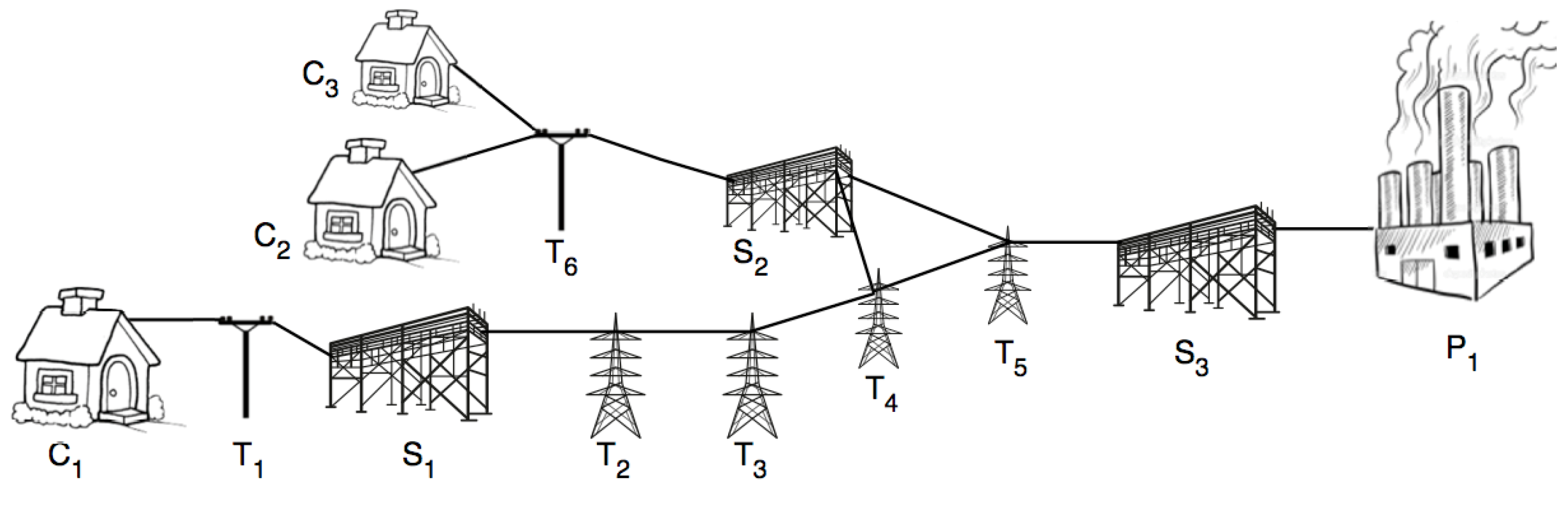
Transmission load for delivering electricity from power plants to consumers varies according to their location in an electric power grid. Yet, the kWh-based analysis does not separately consider the transmission load, so that the environmental impact of electricity transmission (as we will illustrate below) needs to reflect the different transmission distance. Figure 1 illustrates a simple example of the cost-benefit mismatch in an electricity energy system. In Figure 1, electric power is generated at a power plant (P₁) and transmitted to the consumers (C₁ to C₃) through substations (S₁ to S₃), transmission cables, and towers (T₁ to T₆). Consumer C₁ takes electricity from the local substation S₁. On the other hand, electricity for consumer C₂ and C₃ is supplied through the local substation S₂. As each consumer used different transmission facilities, the environmental impact of transmission should be allocated differently according to the transmission facility occupancy rate. For instance, since the electricity transmission flows from the right to the left in the system in Figure 1, substation S₁ and tower T₁, T₂, and T₃ play their role only for the consumer C₁. Therefore, C₁ should take responsibility for the environmental impacts of S₁, T₁, T₂, T₃, and transmission cables between them. However, the conventional kWh-based unit allocates the environmental impact by using only the amount of electricity consumed, and the different transmission load cannot be reflected. Consequently, the structure-dependent transmission load is ignored and it is impossible to estimate the proper environmental impact in an electricity energy system.

Figure 1. An example of an electricity energy system. P symbolizes production, C consumers, T power-grid towers and S substations.

Figure 1. An example of an electricity energy system. P symbolizes production, C consumers, T power-grid towers and S substations.

In this study, we develop a method for allocating the environmental burden of electricity transmission loss. We introduce energy distance to include the individual transmission load of the electricity consumer in an environmental impact analysis. As a case study, we estimate the regional life cycle greenhouse gas (GHG) emissions from electricity consumption in Chile. At first, we analyze the total life cycle GHG emissions of the Chilean electricity energy system in 2012. The GHG emissions are estimated by the life cycle assessment (LCA) method. Then, we convert the total GHG emissions into the transmission load based on the transmission loss ratio. Finally, we allocate the GHG emissions of transmission loss to provinces in two different ways by using the conventional kWh-based unit and energy distance, respectively. The result shows the effectiveness of energy distance in comparison with the kWh-based unit.

2. Method

2.1. Goal, Scope, and Functional Unit Definition

The goal of this study is to estimate the life cycle GHG emissions of transmission loss and allocate this cost to the users of the electricity. Restricted by data availability, we set the geographical and temporal scopes to Chile in the year 2012. We use energy distance as an allocation unit instead of a kWh-based unit. Specifically, we allocate the total GHG emissions of transmission loss to each substation proportional to energy distance, so that substations could be assigned with an environmental burden including both the amount of electricity consumption and the transmission system load.

Since the detailed information, such as the topology of the distribution network and the consumption data of individual users are not available, we consider a substation as a group of users. Functional unit of this study is electricity transmission losses of a province in Chile for one year and we allocate the GHG emissions by the energy distance. We compare the result with the one by the conventional method in which the GHG emissions are allocated by electricity consumption.

2.2. Data Collection and Assumptions

We collect inventory data from the year 2012 regarding the electricity energy system in Chile. Specifically, generation mix, the conversion factor for transmission loss, population of provinces, the connection configuration of transmission lines, and the number of power plants, substations, and towers for life cycle inventory analysis are collected from the year 2012. However, the amount of electricity generation is generalized from the six-year time span. It is because a power plant could stop working for an entire year for maintenance. If inventory data are collected from a specific year, it could distort the results of our study. Therefore, we collect generation data from 2007 to 2012 to obtain the generalized electricity production data. Among the six-year generation and consumption data, we select median values in order to avoid using the extraordinary events such as momentary operation stopping for maintenance. Except for the electricity generation, the other data for life cycle inventory analysis are collected for the year 2012.

The major electric power company in Chile is Centro de Despacho Económico de Carga del Sistema Interconectado Central (CDEC-SIC, Spanish for Economic Load Dispatch Center of the Central Interconnected System). It supplies electricity to more than ninety percent of the population [17]. We set the system boundary to regions where CDEC-SIC supplies electricity. Our regional system boundary covers region III to X, XIV, and RM as listed in Table 1. Region II consumes electricity from not only CDEC-SCI but also SING such that region II is excluded from the system boundary. Seven kinds of power plants are included in the system boundary: coal, hydro reservoir, hydro run-of-river, diesel, natural gas, wind, and biomass. Therefore, we collect inventory data regarding the seven power plants and transmission facilities for six years from the annual CDEC-SIC report [17] and energy statistics report [18]. The detailed statistics of the regions in the system boundary are described in Table S1.

Table 1. Included regions in the system boundary.

Code	Region	Capital city	Area (km2)	Population
III	Atacama	Copiapó	75,176.20	290,581
IV	Coquimbo	La Serena	40,579.90	704,908
V	Valparaíso	Valparaíso	16,396.10	1,723,547
RM	Santiago Metropolitan	Santiago	15,403.20	6,683,852
VI	Libertador General Bernardo O’Higgins	Rancagua	16,387.00	872,510
VII	Maule	Talca	30,296.10	963,618
VIII	Bío Bío	Concepción	37,068.70	1,965,199
IX	La Araucanía	Temuco	31,842.30	907,333
XIV	Los Ríos	Valdivia	18,429.50	363,887
X	Los Lagos	Puerto Montt	48,583.60	785,169

Table 1. Included regions in the system boundary.

Code	Region	Capital city	Area (km2)	Population
III	Atacama	Copiapó	75,176.20	290,581
IV	Coquimbo	La Serena	40,579.90	704,908
V	Valparaíso	Valparaíso	16,396.10	1,723,547
RM	Santiago Metropolitan	Santiago	15,403.20	6,683,852
VI	Libertador General Bernardo O’Higgins	Rancagua	16,387.00	872,510
VII	Maule	Talca	30,296.10	963,618
VIII	Bío Bío	Concepción	37,068.70	1,965,199
IX	La Araucanía	Temuco	31,842.30	907,333
XIV	Los Ríos	Valdivia	18,429.50	363,887
X	Los Lagos	Puerto Montt	48,583.60	785,169

The total amount of electricity generation is larger than the one of consumption in order to compensate the transmission loss, power plants’ own consumption and a sudden peak demand. Electricity is lost during transmission as heat and power plants also consume electricity to operate the facilities. We estimate the amount of transmission loss as seven percent of the total electricity generation [19]. Since the power plant’s self-consumption for the facility operation is less than one percent of the total generation [17], we neglect the self-consumption of power plants. It is common to consider the electric power grid as a flow network satisfying Kirchoff’s circuit law [20]. Accordingly, we assume that the net electricity generation is equal to the consumption in the Chilean power grid network. In our model, only power plants generate electricity and substations consume all the generated electric power. Towers do not affect the system in terms of the amount of electric power.

A local substation distributes electricity to the connected local consumers. However, we assume that a substation consumes electricity as much as the sum of its local consumers do. It is partially due to the lack of information of distribution network and the purpose of this study, which is to develop a method to reflect transmission distance. Note that a substation represents the group of consumers who are supplied electricity distributed from the substation. The detail inventory data about the amount of electricity consumption in the system boundary are listed in Tables S1 in the Supplementary Material.

2.3. Inventory Analysis

2.3.1. Network Analysis

Transmission load of electricity can be analyzed by using network theory. Network theory is used in the area of computer science, network science, statistical physics, etc. and is related to graph theory of mathematics. Network theory analyzes properties of an individual node such as centrality and functionality, or global properties such as robustness and vulnerability of a network [21]. Since network theory takes a pattern or unique characteristics into account from the complex graph, it is applied to study an air transportation network [22], efficiency of wireless networks [23], vulnerability analysis of electricity grid [24], communications at a social network service [25], disease spreading [26], etc. Previously, Lim et al. [27] applied graph theory to calculate transmission loss. They use what they call a “loop-based allocation”, which is a purely topology-based approach, not separating consumption and supply of electricity. For our purpose, to fairly allocate the transmission costs, we need a more detailed picture of the losses. Therefore, our model of transmission loss is more detailed with an explicit separation of supply and consumption.

We construct the network model of Chilean electric power grid. Parts of the life cycle inventory data such as the length and number of lines of the transmission lines between power plants, towers, and substations and the amount of electricity generation and consumption of each node are used to construct power grid network. Power plants, towers, and substations are represented as nodes and each node is connected with other nodes through transmission cables, which are represented as edges in the network model. Every edge has weight as the number of cables multiplied by the length of it. We set the coordinate of nodes as the actual location of each facility in Chile with a minor rearrangement for a better visibility.

Electricity is an energy commodity that flows through electric power grid lines. When an analysis estimates environmental impacts of moving agents or commodity, the estimation could consider not only the amount of commodity but also the distance of transportation. For instance, an LCA study for personal commuting set the estimation unit as “person kilometer” to consider both the number of passengers transported and the distance of transportation [28]. Since electricity energy can be quantified and transported, it is reasonable to consider electricity as a moving commodity as well.

We developed energy distance as the allocation base for this study inspired by the “MW mile” concept of electric engineering [29]. It is designed to involve not only the amount of electricity consumed, but also the transmission distance (Equation 1). Energy distance of a consumer is the sum of the amount of electricity consumed multiplied by the transmission distance from power plants.

$$E{D}_i ={\displaystyle \sum }_j{a}_{ij}\times d_{ij}$$

(1)

where i is a consumer node, j is a power plant node which supplies electricity to i, ED_i is Energy distance of i, a_ij is the amount of electricity transmitted from j to i, d_ij is the transmission distance from j to i. Note that energy distance is measured by the unit of kWh·km for its purpose of considering both consumption and transmission.

Estimating the transmission distance is difficult because electricity flows through a complex power grid network. In order to solve the complexity, we integrate network theory to analyze the transmission distance of electricity. We design network algorithm that the electricity flows through the shortest path as the most efficient way. Each substation finds the nearest available power plant that still has electric power to supply. If a substation demands electricity more than the supply capacity of the nearest available power plant, the substation takes electricity as much as the power plant’s capacity firstly. Afterward, the substation finds the next available power plant. The transmission pair of which transmission distance is shorter than other pairs has the priority of transmission to reduce the total transmission load of the system (see Supplementary Material for the detailed algorithm).

2.3.2. Inventory Allocation

We allocate the inventory of electricity to individual substations in order to estimate provincial GHG emissions due to transmission loss. The inventory for electricity transmission loss is the part of the total inventory for Chilean electric power system. The ratio of transmission loss inventory to the total inventory is proportional to the amount of electricity lost during transmission among the total electricity generated

$$E_{trans}=E_{total}\times r_{trans}$$

(2)

$$IN{V}_{trans}=IN{V}_{total}\times r_{trans}$$

(3)

where E_trans is the amount of electricity corresponding to transmission loss, E_total is the total amount of electricity generation, INV_trans is the inventory of electricity transmission loss, INV_total is the total inventory of electricity generation, and r_trnas is the ratio of the amount of transmission loss among the total amount of generated electricity (we use r_trnas = 0.07 [19]). In reality, transmission loss ratio varies for individual transmission lines with the physical condition such as temperature, voltage, reactance, and impedance of the transmission lines. For the sake of simplicity, however, we assume that all transmission lines have the same conditions.

The allocation of transmission loss inventory to individual substations is on the basis of two different units, the kWh-based unit and energy distance. The inventory of transmission loss of a province allocated by energy distance is

$$IN{V}_{ED\left(i\right)}=\frac{IN{V}_{trans}\times E{D}_i}{{{\displaystyle \sum }}_{i}E{D}_i}=\frac{IN{V}_{trans}\times {{\displaystyle \sum }}_j{a}_{ij}\times d_{ij}}{{{\displaystyle \sum }}_j{{\displaystyle \sum }}_j{a}_{ij}\times d_{ij}}$$

(4)

and, the one by electricity consumption is

$$IN{V}_{CS\left(i\right)}=\frac{IN{V}_{trans}\times a_i}{{{\displaystyle \sum }}_i{a}_i}$$

(5)

where INV_ED(i) is the corresponding electricity inventory of the node i allocated by energy distance, ED_i is the energy distance of node i, and α_i is the amount of electricity consumption of node i. Note that energy distance and the amount of electricity consumption is used for allocation of not the total inventory but the inventory for transmission loss.

2.4. Life Cycle GHG Emissions Assessment

We calculate the life cycle GHG emissions (kg CO_2-eq.) in Chilean electricity energy system from LCA dataset (kg CO_2-eq./kWh) multiplied by the amount of electricity generation (kWh) in Chile. We develop the specific LCA dataset for Chile. LCA dataset is a conversion factor, which indicates how much GHG emissions are occurred per unit of electric power. Itten R., Frischknecht R. and Stucki M. published LCA dataset of Chilean electricity country mix [13]. However, the LCA dataset is based on the inventory data from International Energy Agency in 2009. Since we set the temporal scope for the status of Chilean electric grid in 2012, the LCA dataset should fit into 2012. Therefore, we modified the reference LCA dataset, Ecoinvent 2.2 system processes [13], according to the Chilean electricity generation mix in 2012 (Table 2) as listed in Table 3. Due to lack of detailed information about infrastructures, we do not include it in our calculation. However, it does not cause significant change in our results because the GHG emissions of infrastructure are very lower than the operational emissions (four percent in UK [16]). As LCA analysis tool, we used SimaPro software [30] and IPCC GWP factor [31] for the methodology.

Table 2. Generation mix in 2012 of Chilean electrical power.

Generation type	Generation (GWh)	Ratio (%)
Wind	325.104	0.64
Natural	13,449.271	26.61
Hydro run of the river	7945.923	15.72
Hydro reservoir	14,385.373	28.46
Diesel oil	1357.803	2.69
Biomass	1012.860	2.00
Coal	12,072.210	23.88
Total	50,548.544	100.00

Table 2. Generation mix in 2012 of Chilean electrical power.

Generation type	Generation (GWh)	Ratio (%)
Wind	325.104	0.64
Natural	13,449.271	26.61
Hydro run of the river	7945.923	15.72
Hydro reservoir	14,385.373	28.46
Diesel oil	1357.803	2.69
Biomass	1012.860	2.00
Coal	12,072.210	23.88
Total	50,548.544	100.00

Table 3. Generation mix in 2012 of Chilean electrical power. The LCA dataset used here are Ecoinvent 2.2 system processes [13].

LCA dataset	Amount (kWh)
Electricity, hard coal, at power plant/UCTE	0.239
Electricity, oil, at power plant/UCTE	0.027
Electricity, natural gas, at power plant/UCTE	0.266
Electricity, hydropower, at run-of-river power plant/ RER	0.157
Electricity, at cogen 6400kWth, wood, allocation exergy/CH	0.020
Electricity, hydropower, at reservoir power plant, not alpine region/RER	0.285
Electricity, at wind power plant/ RER	0.006
Electricity, production mix CL/kWh/2012	1.000

Table 3. Generation mix in 2012 of Chilean electrical power. The LCA dataset used here are Ecoinvent 2.2 system processes [13].

LCA dataset	Amount (kWh)
Electricity, hard coal, at power plant/UCTE	0.239
Electricity, oil, at power plant/UCTE	0.027
Electricity, natural gas, at power plant/UCTE	0.266
Electricity, hydropower, at run-of-river power plant/ RER	0.157
Electricity, at cogen 6400kWth, wood, allocation exergy/CH	0.020
Electricity, hydropower, at reservoir power plant, not alpine region/RER	0.285
Electricity, at wind power plant/ RER	0.006
Electricity, production mix CL/kWh/2012	1.000

In Section 2.3.2, we allocate inventory to substations based on two different allocation bases. Consequently, we compare the distribution of the allocated regional GHG emissions of transmission loss from the two different units. The comparison reveals the effectiveness of energy distance for the allocation purpose. See Section 3.3 for the detailed results and discussion.

In addition, we calculate the specific GHG conversion factors for the provinces. The regional GHG emissions are divided by the amount of electricity consumption in each province. The result generates the site-specific GHG conversion factors, kg CO_2-eq. per kWh, for provinces.

3. Results and Discussion

3.1. Chilean Electric Power Grid Network

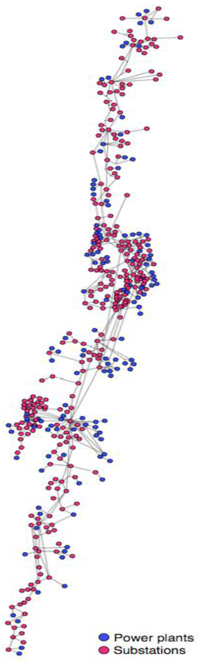
Chilean electric power grid consists of in total 466 nodes including 129 power plants and 291 substations. The network map is drawn in Figure 2. Red nodes represent substations and blue nodes are power plants. The lines between nodes are transmission cables between power plants, substations, or towers. The coordinates of nodes and edges are illustrated as the actual locations. The method and rules for generating Chilean power grid network from the real data (Tables S2–S4), the final edge list (Table S5), and the final node list (Table S6) are in Supplementary Material with corresponding inventory data.

Figure 2. Network model of Chilean electric power grid. Blue circles represent power plants and red circles for substations. Lines between circles are the transmission line connecting the two nodes.

Figure 2. Network model of Chilean electric power grid. Blue circles represent power plants and red circles for substations. Lines between circles are the transmission line connecting the two nodes.

A node can be analyzed based on how much central the node’s function is. For instance, when the sum of distances from a node to the other nodes in the network is shorter than any other nodes, the node has the highest closeness centrality.

However, in an electricity network, high closeness centrality of a substation does not always guarantee high accessibility to power plants. Since closeness centrality is a global centrality to the whole nodes in a network, it cannot represent the centrality in the specific supply-demand relationship. Hence, we measure energy distance in a specific set of power plant and substation pairs.

3.2. Transmission Load Analysis

We designed an algorithm to decide a transmission pair of a power plant and a substation. The algorithm is under the assumption that the electric power grid has been developed to the direction of increasing its efficiency. On the efficient electric power grid, electricity transmission pairs are set of which total transmission load is lower than other configurations. In order to verify whether the algorithm generates an efficient set of transmission pairs, we used simulated annealing optimization [32]. Simulated annealing is a generally applicable optimization technique for problems with many local extrema. The result of simulated annealing confirms that the transmission pairs are made up of the lowest total transmission load. However, it should be noted that the real total transmission load might not be the lowest. For example, electricity energy system could have a surplus of facilities to ensure the system security or a dispatch center could control electricity distribution manually through a long-distance path to respond to instant peak demands.

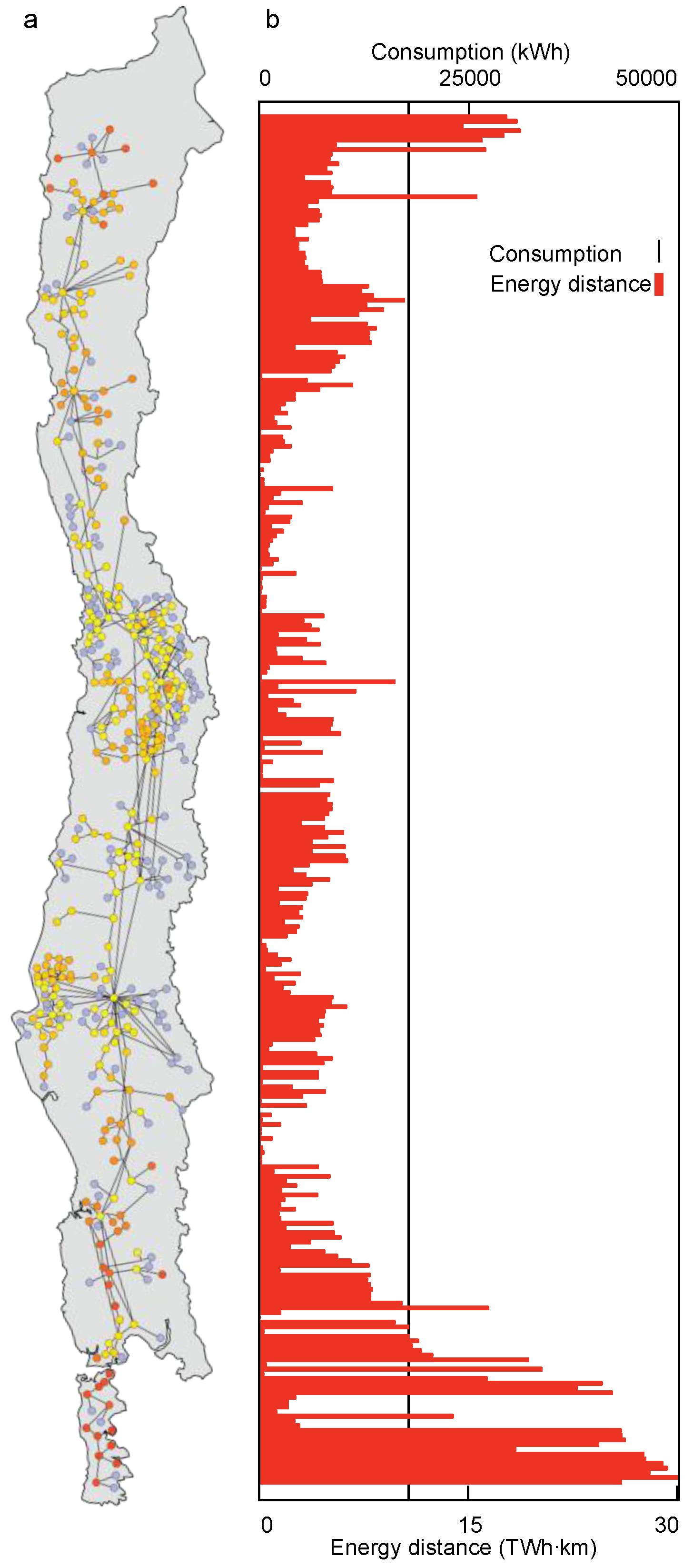
In order to analyze how energy distance can reveal the transmission load, we set an arbitrary situation distributing the total amount of electricity consumption to all substations equally. Figure 3a,b shows the distribution of electricity consumption and energy distance in the arbitrary situation. The substation nodes are colored from yellow to red according to increasing energy distance in Figure 3a. The nodes located at the end of country have larger energy distance because the nodes require the longer transmission distance than the central nodes.

If we assume that substations take responsibility for the environmental impacts from the electric power system according to the amount of consumption, as the conventional LCA analyses do, all substations induce environmental impacts identical as the straight consumption line in Figure 3b. However, when the environmental impacts are distributed proportional to energy distance, the level of inducement varies according to both the substations’ transmission distance and amount of consumption (Figure 3b). The result shows that energy distance is effective to reflect transmission load.

The ratio of transmission loss directly affects the GHG emissions calculation. Considering the general trend of the transmission loss ratio of the Chilean power grid—8.49 ± 1.70 percent of loss for 20 years until 2012—the 7.13 percent ratio in 2012 stays within the 20-year trend, which means that the 7 percent can represent the general performance of the Chilean power grid. However, there is room for improvement of the results. For example, the amount of current flow between substations and power plants and the input and output electric power at each node can provide the amount of the transmission loss for each transmission line, which results in the more realistic analysis. Power grid data such as the number of power plants, the amount of generation, and the position of power plants are also critical to the results. Since we use all the values for the power grid data in 2012, note that the results are limited only for the temporal and spatial scope of this study.

Figure 3. (a) Chilean electricity grid network (b) the distribution of energy distance in the arbitrary situation.

Figure 3. (a) Chilean electricity grid network (b) the distribution of energy distance in the arbitrary situation.

3.3. Comparison: Impact Analysis and Regional Allocation

The annual electricity consumption in the system boundary is 50.28 TWh [18]. LCA dataset converts 1 kWh of electricity consumption of Chilean national grid mix to 0.459 kg CO_2-eq. of GHG emissions. Therefore, the total GHG emissions of the Chilean electric power grid is 23.07 Mt CO_2-eq. and the total energy distance is estimated to be 12,842.10 TWh km. The GHG emissions of the transmission loss of the Chilean electric power grid is 1.61 Mt CO_2-eq..

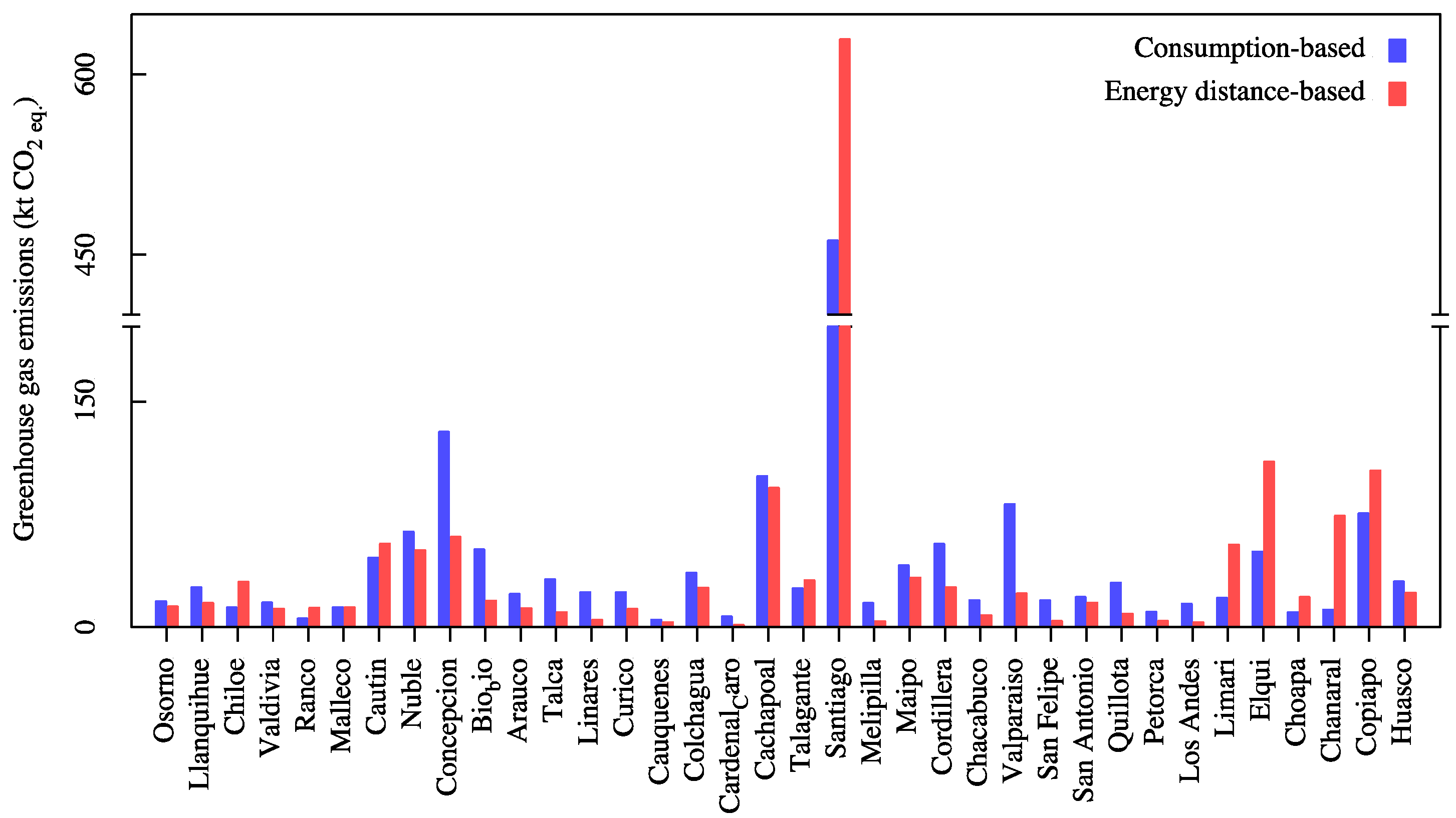
We allocated the GHG emissions of the transmission loss by province with the allocation unit of energy distance. Chile is divided into 15 regions. Among the regions, 10 regions are included in the system boundary. A region consists of several provinces, which are second-level administrative division of Chile. Figure 4 shows the distribution of GHG emissions calculated based on energy distance (red) and electricity consumption (blue), respectively. Each bar in the graph represents the GHG emissions of each province and is plotted from the southern to the northern location.

Figure 4. GHG emissions of the transmission loss allocated by energy distance (red) and electricity consumption (blue). Energy distance-based allocation results in the different distribution to the provinces.

Figure 4. GHG emissions of the transmission loss allocated by energy distance (red) and electricity consumption (blue). Energy distance-based allocation results in the different distribution to the provinces.

Energy distance and electricity consumption result in the different distribution of the environmental cost of GHG emissions for transmission loss. When the amount of electricity consumption is used as an allocation unit, the capital region Santiago is allocated the most GHG emissions. The second GHG emitter province is Concepcion, to which the most industrialized city in Chile belongs. The third ranked province, Cachapoal, is the fifth most populated in Chile. The fourth GHG emitting Valparaiso is the third largest province in Chile and includes one of the most important seaports in it. The large population or high industrial level induces a large amount of electricity consumption. Naturally, the large amounts of GHG emissions are allocated to these provinces proportionally to the electricity consumption.

However, when energy distance is applied as the allocation unit, the distribution is changed. The first GHG emitter driven from energy distance is the same as the case of kWh. However, for example, Elqui increases from the province contributing ninth most to the GHG emissions to second ranked province. Concepcion, however, becomes sixth ranked although it consumes more than Elqui. This is because energy distance considers the network configuration to calculate transmission load. Even though Concepcion consumes more than twice the electricity of Elqui (4.04 TWh and 1.56 TWh, respectively), since many local power plants are installed around Concepcion, energy distance of Conception is about half of Elqui (477.13 TWh km and 875.46 TWh km, respectively). As a result, the net GHG emissions of transmission loss for Conception becomes lower than the one of Elqui. The ranks of GHG emissions of provinces are listed in Table 4 for top 10 provinces and in Table S7 for the entire list.

Table 4. Ranks for GHG emissions of transmission loss of provinces (top 10).

Province	GHG Emissions Rank by		Energy Distance (TWh km)
	Electricity Consumption	Energy Distance
Santiago	1	1	5001.68
Concepcion	2	6	477.13
Cachapoal	3	4	735.91
Valparaiso	4	16	176.43
Copiapo	5	3	826.93
Nuble	6	9	404.32
Cordillera	7	13	210.27
Bio Bio	8	18	138.48
Elqui	9	2	875.46
Cautin	10	7	440.39

Table 4. Ranks for GHG emissions of transmission loss of provinces (top 10).

Province	GHG Emissions Rank by		Energy Distance (TWh km)
	Electricity Consumption	Energy Distance
Santiago	1	1	5001.68
Concepcion	2	6	477.13
Cachapoal	3	4	735.91
Valparaiso	4	16	176.43
Copiapo	5	3	826.93
Nuble	6	9	404.32
Cordillera	7	13	210.27
Bio Bio	8	18	138.48
Elqui	9	2	875.46
Cautin	10	7	440.39

For the sake of the case that one may need the conventional form of GHG conversion factor (g CO₂ per kWh), we derive the regional GHG conversion factors dividing the GHG emission burden by the amount of electricity consumed in each province (see Supplementary Material). Table S8 shows the amount of electricity consumption by province. The result shows the specific GHG conversion factors for Chilean provinces. The values vary up to two orders of magnitude. The environmental cost of electricity is highest in Chanaral and lowest in Cardenal Caro.

Energy distance is effective especially in the large-scale electric network. Many environmental impact assessment tools do not consider transmission load separately at the moment. It is because the environmental impact from electricity transmission load is complicated compared to the one from electricity generation. Hence, the transmission loss is embedded into the consumption proportional to the electricity generation. However, on the intercontinental scale, electric network such as Asia Super Grid [33,34], Desertec [35], and TuNur [36], the transmission load becomes significant and non-negligible. Moreover, when the electric power sources become more renewable, the environmental impact from electricity generation will decrease. In this sense, it will no longer be reasonable to allocate the environmental impact from transmission loss to the unit of electricity generation equally. Network analysis can provide the comprehensive information for consumers’ load profile in the electric power system. It can be used to allocate not only environmental impacts but also ecological impacts, bio diversity, aesthetic value, or cost of producing and maintaining electricity infrastructure.

4. Conclusions

In this study, we integrated network theory into an environmental impact assessment tool, LCA analysis. We constructed a network model of the Chilean electricity energy system, and used it as a basis for our network-theoretical analysis. Electricity transmission distances between power plants and substations are calculated from a distance-weighted network. The specific LCA dataset for the Chilean electricity energy system is also made from Ecoinvent LCA dataset V3 by modifying its electricity generation mix for the scope of this study, in 2012. The total GHG emissions of the Chilean electricity energy system are estimated based on the standard LCA method with 23.07 Mt CO_2-eq. We used the new allocation unit, energy distance, in order to allocate the total GHG emissions to provinces. The regional GHG conversion factors are calculated for further usage.

This study attempts to apply network analysis to LCA in a simplified way, so it can be extended in many directions. For example, power plants have their own characteristics in the electric power grid. Coal power plants are in charge of meeting peak demand due to their fast operational reactivity in contrast to hydropower plants, which are responsible for the baseline consumption. These various operational roles in the energy system can be considered in future study.

We show that network theory can be applied with LCA analysis providing the quantified functionality or activity of system components. It can be used for the various topics of LCA studies as a way of extracting information from a very complex life cycle or production system. However, since the results of network analysis depend on the network topology and analysis algorithm, a standard method for network model construction and algorithm development will be needed for network theory integration across various topics.