Article

Monocentric or Polycentric? The Urban Spatial Structure of Employment in Beijing

1
School of Geography, Beijing Normal University, No. 19, XinJieKouWai Str., HaiDian District, Beijing 100875, China
2
Urban-Rural Planning Administration Center, Ministry of Housing and Urban-Rural Development of China, No.9 San Li He Road, Beijing 100835, China
*
Author to whom correspondence should be addressed.
Sustainability 2015, 7(9), 11632-11656; https://0-doi-org.brum.beds.ac.uk/10.3390/su70911632
Submission received: 25 May 2015 / Revised: 11 August 2015 / Accepted: 13 August 2015 / Published: 25 August 2015
(This article belongs to the Special Issue Urban Land and Sustainable Development)

Abstract

:
The spatial structure of Beijing has changed dramatically since the reforms of the late 1970s. It is not clear, however, whether these changes have been sufficient to transform the city’s monocentric spatial structure into a polycentric one. This paper uses 2010 enterprise registered data to investigate the spatial distribution of employment in Beijing. Using a customized grid to increase the spatial resolution of our results, we explore the city’s employment density distribution and investigate potential employment subcenters. This leads to several findings. First, Beijing still has strong monocentric characteristics; second, the city has a very large employment center rather than a small central business district; third, five subcenters are identified, including four in the suburbs; and fourth, a polycentric model that includes these subcenters possesses more explanatory power than a simple monocentric model, but by only four percentage. We conclude that the spatial structure of Beijing is still quite monocentric, but may be in transition to a polycentric pattern.

1. Introduction

China is urbanizing at an unprecedented rate, with many cities experiencing rapid population expansion [1]. Beijing, the country’s capital, has been one of its fastest-growing cities over the past few decades [2,3,4]. According to census data, Beijing’s population grew from 13.6 million in 2000 to more than 19.6 million in 2010, an increase of 44.5%. The aggregation of population in the city center has caused many problems, including traffic congestion [5,6], air pollution [7,8,9] and a lack of affordable housing [10,11].
These problems are often blamed on the capital’s spatial structure, which critics argue is overly monocentric and should be decentralized. In fact, Beijing has been making efforts to establish a polycentric urban spatial structure by implementing a series of urban plans and related policies, targeting the decentralization of both employment and population [12,13]. Since the economic reforms of the late 1970s, Beijing has issued three comprehensive city plans, with planning periods of 1981–2000, 1991–2010 and 2004–2020 [14,15]. Each of these plans has included the formation of a multi-center development pattern among its goals. For example, the 1991–2010 Beijing Comprehensive Plan outlined a polycentric development pattern that it called “decentralized cluster style (Fensan Zutuan Shi)”. In this proposal, the urban area would consist of the existing old city and ten edge clusters, each surrounded by a greenbelt (the first greenbelt) that would control urban sprawl and improve environmental quality. With the development of urban land and housing markets since the early 1990s, however, Beijing’s urban area expanded quickly, encroaching on the greenbelt. By the early 2000s, the greenbelt had all been developed, and the old city merged completely with the edge clusters [16]. The 2004–2020 Beijing Comprehensive Plan followed its predecessor’s principle of decentralized development, proposing a three-tier development structure composed of the central city, the new towns and the common towns. The central city referred to the old city and the ten edge clusters from the 1991–2010 plan; the new towns included eleven towns where suburban district and county governments were located [17]; and the common towns referred to other designated towns. Between the central city and the new towns, a second greenbelt was planned with the same purpose as the first.
The city’s spatial structure and these efforts to control it have attracted broad interest from researchers and policy makers. Many studies have focused on the spatial distribution of Beijing’s residential population, concluding that, in general, the city has shown a trend toward polycentricity and suburbanization [18,19,20,21,22,23]. However, just because a city’s residential population has suburbanized does not necessarily mean that its urban spatial structure has also changed to a polycentric form, especially if employment is still concentrated in the city center. The spatial distribution of employment plays an important role in the structuring of urban spaces. Indeed, some urban economic theories begin from the spatial distribution of employment and determine population distribution from distance to the employment center, transport costs and other factors [24,25,26,27]. Thus, a polycentric city is usually defined by the presence of one or more employment subcenters outside of the central business district [28].
Unfortunately, few studies have examined the spatial distribution of employment in Chinese cities, probably due to the difficulty of data collection. China has conducted six population censuses, in 1953, 1964, 1982, 1990, 2000 and 2010, and thanks to the country’s hukou (household registration) system, annual population data are available for most cities. In contrast, the country has conducted only two economic surveys of limited scope, in 2004 and 2008. What is more, data collected in these surveys are of doubtful quality due to the lack of unified classification standards among administrative departments at different levels [29].
These few studies have yielded no consensus. Some researchers suggest that Beijing is still dominated by a monocentric urban spatial structure [30,31], while others conclude that Beijing has already entered a polycentric era [31,32]. For example, Sun et al. [32] use employment data from the secondary and tertiary industries to identify five employment subcenters: Yangfangdian Street, Zhongguancun Street and Shangdi Street in Haidian District, Heping Street in Chaoyang District and Yingfeng Street in Fangshan District. Due to the limitations of existing employment data, these studies were mainly based at the town level, which leads to relatively coarse results [33].
This paper seeks to deepen the understanding of Beijing’s urban spatial structure by using a better set of employment data: the 2010 enterprise registered data from the Beijing Industry and Commerce Bureau. We customize a 1.5 km × 1.5 km grid as the research unit and follow the two-stage method proposed by McMillen [28] to identify employment subcenters. Finally, we establish a polycentric model to explain the employment density distribution. Our findings will supplement the current understanding of the city’s spatial structure and lay the foundation for better urban development, planning and policy-making in the future.
The paper is organized as follows: Section 2 describes the research area, data and method, while Section 3 provides a general description of employment density in Beijing in 2010. Section 4 evaluates a monocentric model, identifies Beijing’s employment subcenters and examines the subcenters’ ability to explain the entire employment density distribution of the city. Conclusions are presented in Section 5.

2. Research Area, Data and Methods
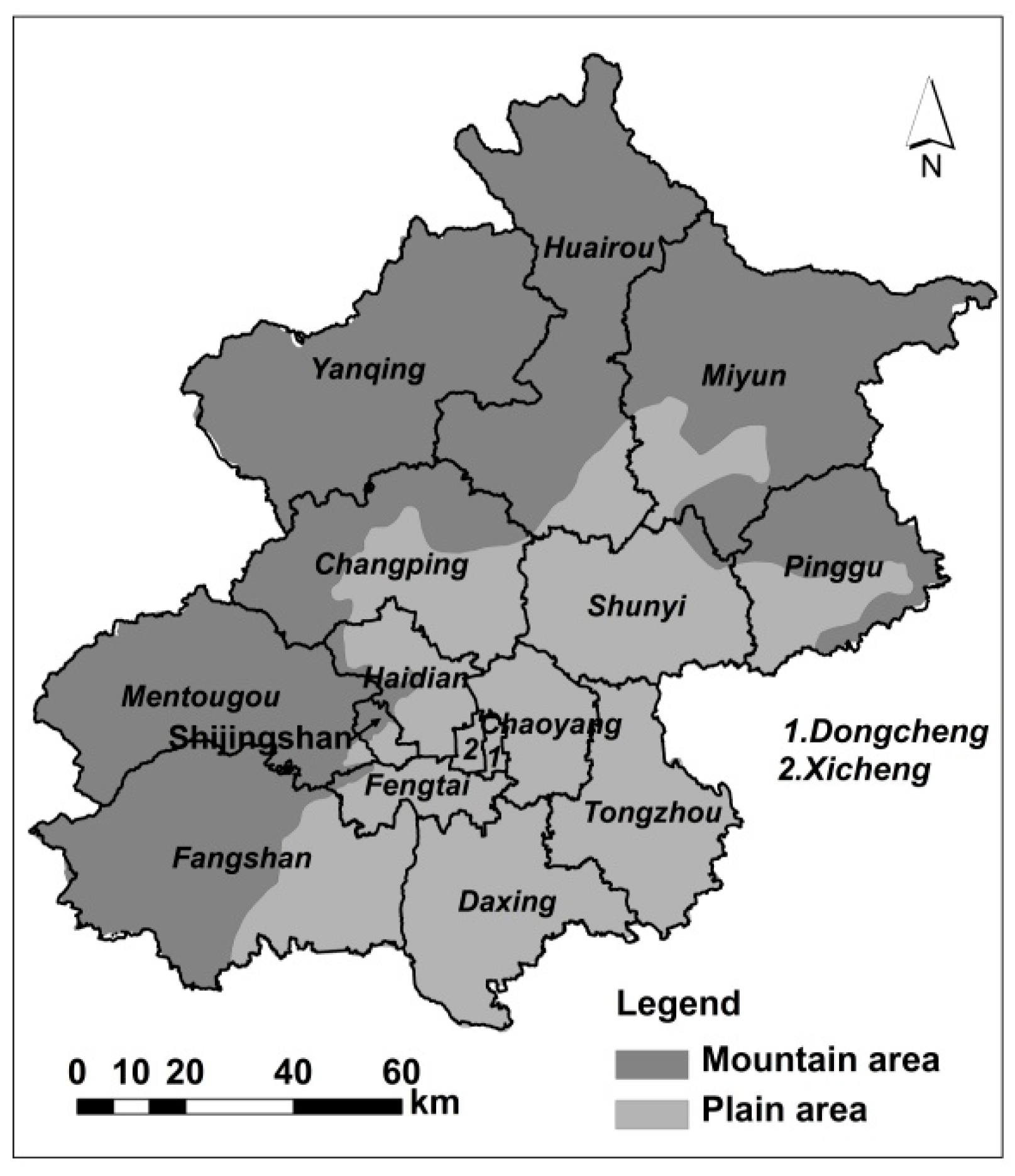
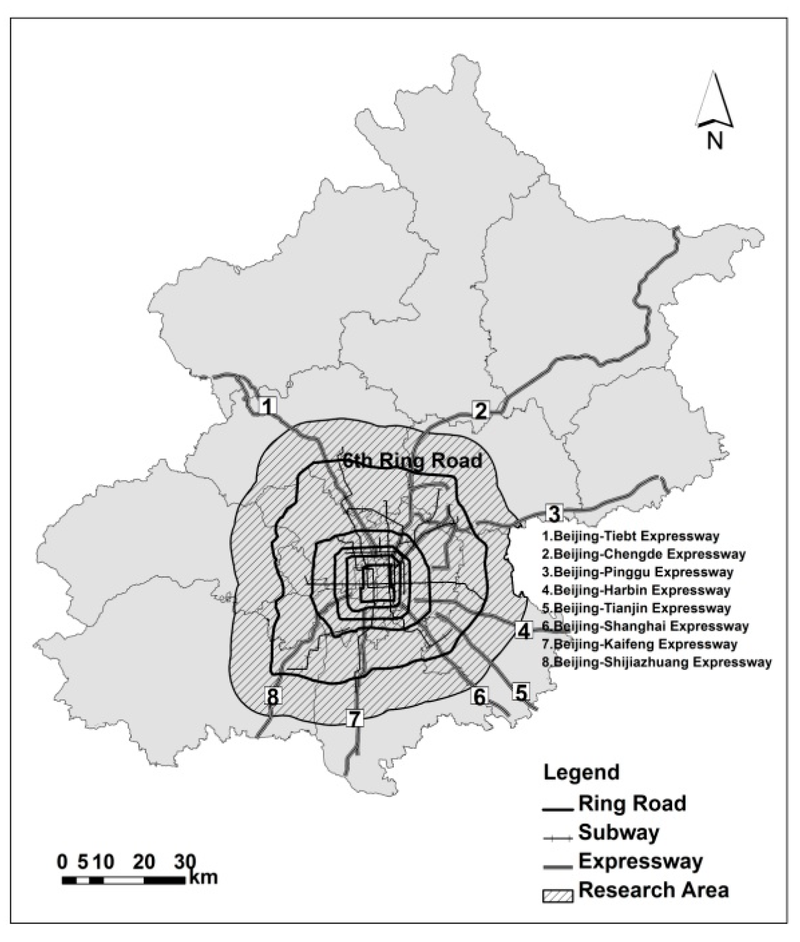
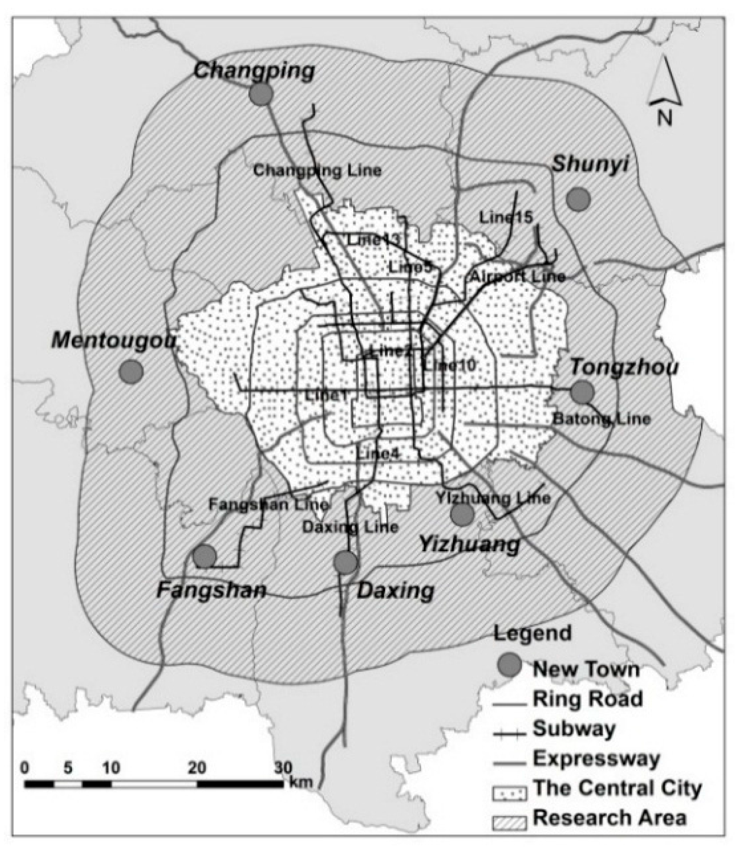
2.1. Research Area

Beijing has a total administrative area of approximately 16,410 km2. The city’s northwest is a primarily mountainous area of about 10,072 km2 and is protected for ecological reasons, while the southeast is made up of plains of about 6338 km2 (Figure 1). The main urban area is located on this plain, with the Ming and Qing Dynasty Imperial Palace (the Forbidden City) at its center. Since 1949, a system of ring roads has been developed around the Forbidden City, with the city’s expansion requiring the construction of the 2nd, 3rd, 4th, 5th and 6th Ring Roads in turn [34]. With Tiananmen as the center, the average radius of these five ring roads is about 4 km, 7 km, 10 km, 15 km and 25 km, respectively. Eight radial expressways have also been constructed to link the central city and suburban areas (Figure 2). The city’s subway system is a similar ring-and-radial network; Subway Lines 2 and 10 are loop lines, while Lines 13 and 4, as well as the Changping, Fangshan, Yizhuang, Shunyi, Batong and Airport lines are all radial lines.
Figure 1. Topographic map of Beijing.
Sustainability 07 11632 g001
Figure 2. Research area of the study.
Sustainability 07 11632 g002
We define a research area of 4429 km2, which includes the area within the 6th Ring Road and a 10-km buffer zone beyond it (Figure 2). We selected this research area based on several considerations. First, in view of the subway system’s extent and assumptions about the commuting range of private cars, this area represents a reasonable commuting scope and can be regarded as an integrated labor market. Indeed, according to bus-pass data, the majority of transportation flow occurs within this area [35]. Second, the research area includes not only the central city, but also seven new towns, which have closely integrated with it [36] (Figure 3). Third, this area accommodates most of Beijing’s population and firms, accounting for about 80.9% and 74.5%, respectively. Fourth, if the research area were expanded further, many mountainous regions with weak links to the central city would be included.
Figure 3. The Central city and planned new towns.
Sustainability 07 11632 g003

2.2. Data

The employment data are from the Beijing Industry and Commerce Bureau’s 2010 list of registered enterprises and institutions. The registered enterprises include state-owned, private, collective, foreign-invested, foreign-owned and other types of enterprise, while the institutions include government agencies, institutions and social organizations. Collected information includes enterprise and institutional names, addresses, turnover, registered capital, the number of their employees, and so on. We use ArcGIS and Google Maps to locate the enterprise address, giving us the spatial location of all 411,300 enterprises [37].
The Beijing Industry and Commerce Bureau’s dataset includes 14.91 million employees, the sectoral composition of which is in general accordance with the published data of the Beijing Statistical Yearbook [38] (Table 1). This dataset covers a wide range of industries; business services, technological exchange and promotion services and wholesale trade are the top three by employment, accounting for 6.3%, 5.9% and 5.8% of the total employment, respectively (Table 2).
One shortcoming of our data is that the employment figures for some large enterprises, such as the China National Tobacco Corporation, the China Network Communications Group Corporation and Sony (China) Limited, include employees working not only in Beijing, but also elsewhere in China. If these companies are included in the study, they might bias the spatial distribution of employment in the research area. Therefore, we eliminated 560 companies of this kind from the dataset, representing 0.14% of the total number of enterprises in the research area [39]. Due to their relatively small numbers and lack of spatial concentration, excluding these enterprises has little effect on our results. Because of these removals, the dataset used in this study contains 410,800 enterprises and 13.51 million employees.
Table 1. Composition of employment by sector.
Data SourcePrimary IndustrySecondary IndustryTertiary Industry
Beijing Statistical Yearbook6.0%19.5%74.4%
Beijing Industry and Commerce Bureau1.6%22.3%76.1%
Table 2. Top ten industries by number of employees.
Top Ten IndustriesEmploymentPercentage of Total Employment
Business services942,9576.3%
Technological exchange and promotion services878,8095.9%
Wholesale trade857,6815.8%
Education575,3603.9%
Construction545,5893.7%
Retail Trade527,9123.5%
Real estate458,4343.1%
Computer service industry348,7452.3%
Catering trade340,7992.3%
Health315,5352.1%
Top ten total5,791,82138.8%

2.3. Methods

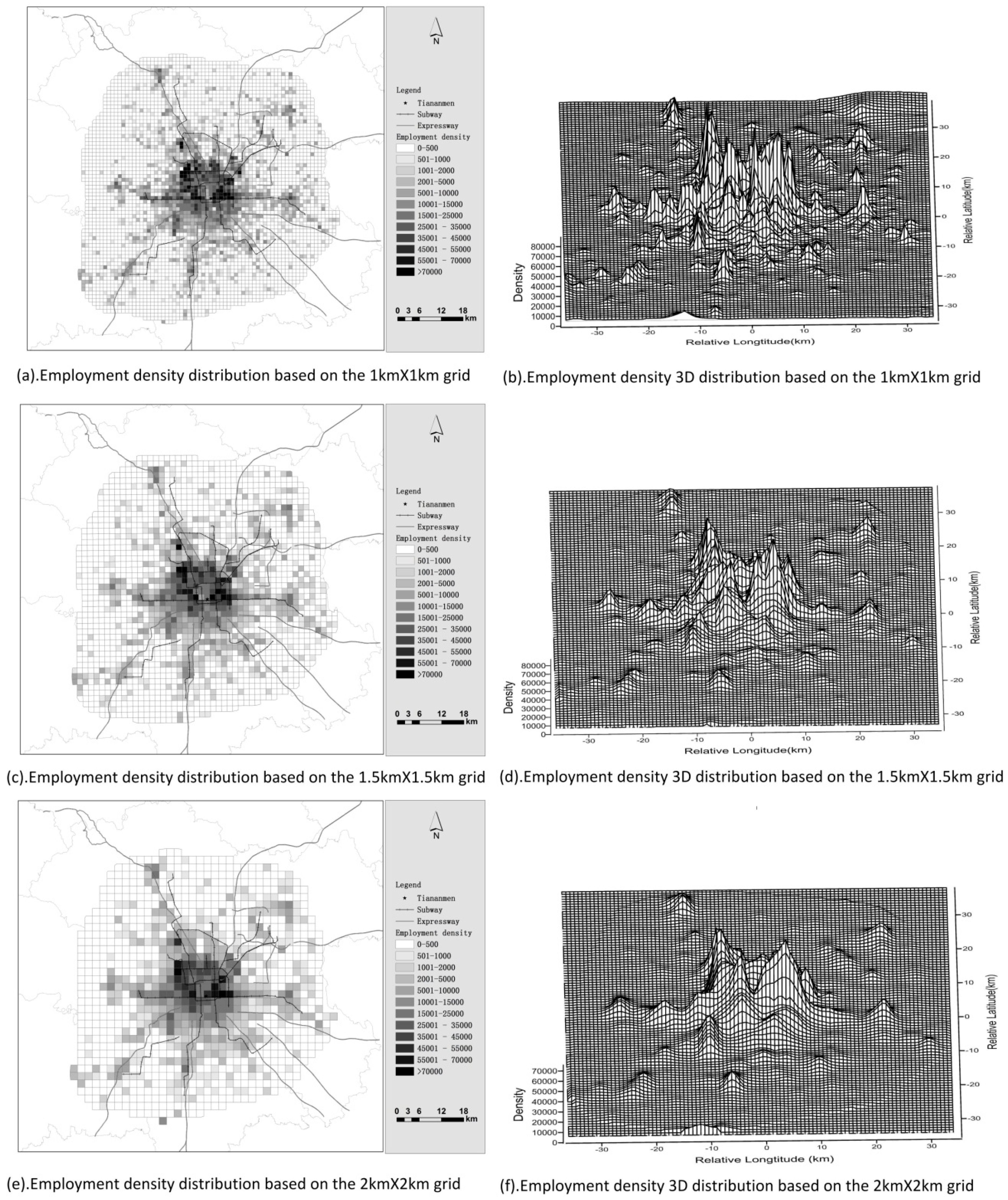
2.3.1. Defining the Research Unit

The research area includes 195 towns (townships or streets), with an average administrative area of about 22 km2. Towns are, therefore, too large to make an effective research unit by the standards established in the literature. For example, McMillen et al. [40] use 0.5 square miles (about 1.29 km2) of a statistical sample as their research unit; McDonald et al. [41] use 1 square mile (about 2.56 km2); and Giuliano et al. [42] use an average of 3 square miles as their research unit. In light of these scales, we defined a customized grid as our research unit.
Choosing the appropriate grid size is critical and can affect the calculated employment density. If the grid is too small, there will be many units with zero employment density, such as parks or residential blocks, and many others with extremely high employment density, such as blocks of high-rise office buildings. If the grid is too large, employment concentrations may be offset by neighboring parks, and centers of employment may be hard to identify [28].
We tested grids with cell sizes of 1 km × 1 km, 1.5 km × 1.5 km and 2 km × 2 km [43]. As shown in Table 3, the research area includes 4266 cells of 1 km × 1 km with 24.9% of them being null, 1883 cells of 1.5 km× 1.5 km with 9.2% of them being null and 1030 cells of 2 km× 2 km with 6.5% of them being null (Table 3). Considering both the number of samples and the percentage of null-value units, we chose to use the 1.5 km × 1.5 km grid as our research unit.
Table 3. Grid sizes compared.
Grid Cell SizeStudy Unit NumberNull Value UnitEmployment Density (Person/km2)
NumberPercentageMaxMinMean
1 km × 1 km4266106224.9%114,85024767
1.5 km × 1.5 km18831739.2%98,74623822
2 km × 2 km1030676.5%93,53823670

2.3.2. Identifying Subcenters

A number of methods have been used to identify subcenters in metropolitan areas. Among them, the most direct relies on the researcher’s knowledge and observations, but this is highly subjective. Building on observations and experience, some researchers use a threshold value-setting method for identifying employment subcenters. For example, Giuliano et al. [42] define a subcenter as a group of contiguous tracts that each have at least 10 employees per acre and that together have at least 10,000 employees. This method is also subjective, since the identification of subcenters is sensitive to the choice of the threshold. For example, McMillen et al. [44] use a threshold of 20 people/acre, with total employees exceeding 20,000.
McDonald [45] proposed a more objective method for identifying employment subcenters, defining a subcenter as a cluster of significant positive residuals from a simple regression of employment density on the distance from the central business district. McDonald et al. [41] subsequently used the same method to identify employment subcenters in Chicago, with reasonable results. McMillen [28] argued that a subcenter should also have a significant effect on overall employment in the city and proposed a two-stage method, which first identifies candidate subcenters and then estimates their explanatory power. This two-stage method is better at eliminating subjective influences and can easily be employed by other researchers [28,40].
We adopt a similar two-stage method. In the first stage, we follow McDonald’s [46] method of identifying potential subcenters. First, we establish a monocentric model. The classical monocentric model assumes that all of a city’s jobs are concentrated in its central business district [24,26,27]. However, this assumption cannot fit reality. When investigating the spatial distribution of employment, many studies assume that employment distribution is similar to population distribution, but more concentrated in the city center [47]. To capture this dynamic, a negative exponential model has been widely used.
D s = α e β s + u
D(s) is employment density; s is the distance to Tiananmen, often regarded as Beijing’s center [48]; α is employment density at distance zero and β (β < 0) is density gradient; u is the error term.
Second, since the negative exponential model is nonlinear, we use its logarithmic form to estimate it by the ordinary least squares method (OLS).
L n D ( s ) = β s + c + u
Here, c = lnα, and other symbols are the same as in model Equation (1).
Using this monocentric model, the residuals between real and predicted values can be calculated, and those observations with residuals significant at the 95 percent confidence level are chosen as potential subcenters.
Third, to deal with the potential problem that a unit surrounded by very low employment density units could be falsely identified as a candidate subcenter, we follow the threshold method of Muñiz et al. [49], which uses the average employment density of the research area as the threshold for determining potential employment subcenters.
In the second stage, we build a polycentric model to test whether our candidate subcenters help explain the research area’s overall employment density distribution. Heikkila et al. [50] propose three different hypotheses about the role of subcenters, corresponding to three different polycentric models. As potential subcenters have different industries and different functions [51], the hypothesis that benefits from all subcenters being completely complementary is most suitable for our study. Based on an exponential function, a polycentric model that added control variables can be expressed as:
D ( s , s s u b i , X ) = α 0 e β s e i = 1 n α i s s u b i e δ X e u
where D ( s , s s u b i , X ) is the density of a research unit, s and s s u b i are the distance to Tiananmen and the potential employment subcenter i, respectively; X is control variables, including the distance to the nearest subway station, the highway and the airport; a0, ai(i = 1, 2…) and δ are parameters to be estimated; u is an error term.
A log-transformed version of model Equation (3) is also adopted here, for the same reason. Thus, our polycentric model is as follows:
L n D ( s , s s u b i , X ) = β s + i n α i s s u b i + δ X + c + u
Here, c = lnα0 and other symbols are the same with model Equation (3).
However, many studies suggest that the employment density declines more precipitously when moving away from subcenters than from the main city center; therefore, the inverse distances to the employment subcenters are often employed as interpretation variables [40,46], as shown in model Equation (5). This can also solve the problem of potential collinearity between the distance variables. In our research, model Equation (5) is adopted to estimate the effect of subcenters on overall employment density distribution.
L n D ( s , s s u b i , X ) = β s + i n α i s s u b i 1 + δ X + c + u

2.3.3. Effect of the Potential Subcenter on Local Employment Density

To examine the effect of potential subcenters on local employment density, we estimate regressions with the distance to Tiananmen and the distances to each potential subcenter as the explanative variables and confine the observations to certain scopes (5, 10 and 15 km radius) to the potential subcenters shown in model Equation (6).
L n D ( s , s s u b i ) = β s + α s s u b i + c + u
Control variables are excluded in the above model Equation (6) since distances to subway stations and highways are in general highly correlated with the distance to the subcenters, and the distance to the airport has little effect on the employment density when the observations are limited to a local scope.

3. Employment Density in Beijing

The average employment density in the research area is 3125 employees/km2. There is a great deal of variation around that mean, however, from just two employees/km2 up to a high of 98,746 employees/km2 in one grid cell on Jianguomen Street. The spatial distribution of employment displays four major characteristics as follows.

3.1. Density Declines from the Center to the Suburb

The research area is divided by the five ring roads into six concentric zones, numbered from I, in the center, to VI, on the periphery (Figure 4). Employment density varies among these ring zones, decreasing dramatically as one moves outward from the center. The employment densities of the six zones, from center to periphery, are 29,248 employee/km2, 31,547 employee/km2, 22,571 employee/km2, 6897 employee/km2, 1447 employee/km2 and 563 employee/km2 (Table 4). From the innermost to the outermost ring zone, the employment density drops by about 98%.
Figure 4. The six ring zones.
Sustainability 07 11632 g004
The highest employment density is not observed in the innermost ring zone, but in the next zone out, Zone II, which is not predicted by the classic monocentric model. Several factors may contribute. First, historic-site preservation has prevented economic concentration. The 2nd Ring Road was built at the site of the old city wall and contains within it the city’s major sites of historical and cultural importance, including the Ming and Qing Dynasty Imperial Palace, Tiananmen (which together cover about 1.2 km2), the Temple of Heaven and historic quadrangles and lanes (hutong). Preservation of the old city has long been an important part of city planning, and many important sites have been protected from modern development as a result. Second, development and construction within the 2nd Ring Road are subject to strict planning regulations, such as building height caps and density limits, which have influenced employment density. Third, the city has relocated populations and manufacturing from the center to suburban areas to reduce pressure on the central city.
Table 4. Employment density by ring zone.
Ring ZonesArea (km2)Area Share (Percentage)Enterprise Number Share (Percentage)Enterprise Density (Per km2)Employment Share (Percentage)Employment Density (Per km2)
I (within 2nd Ring Road)62.01.4%11.7%77513.1%29,248
II (between 2nd and 3rd Ring Roads)97.12.2%20.8%87822.1%31,547
III (between 3rd and 4th Ring Roads)141.63.2%23.8%69123.1%22,571
IV (between 4th and 5th Ring Roads)311.77.0%15.6%20615.5%6897
V (between 5th and 6th Ring Roads)1664.637.6%18.3%4517.4%1447
VI (outside the 6th Ring Road)2152.548.6%9.8%198.8%563
Table 5. Cumulative employment density by ring zone.
ZonesArea (km2)Area Share (Percentage)Enterprise Share (Percentage)Enterprise Density (Per km2)Employment Share (Percentage)Employment Density (Per km2)
I (within 2nd Ring)62.01.4%11.7%77513.1%29,248
I + II (within 3rd Ring)159.13.6%32.5%83835.2%30,651
I + II + III (within 4th Ring)300.76.8%56.3%76958.3%26,847
I + II + III + IV (within 5th Ring)612.513.8%71.9%48273.8%16,693
I + II + III + IV + V (within 6th Ring)2269.051.2%90.2%16391.2%5567
Research area4429.6100.0%100.0%93100.0%3125

3.2. A Vast Employment Center

It is also worth noting that the 4th Ring Road seems to be a boundary outside which the employment density plummets, while the employment densities of the areas within the 4th Ring Road (Zones I, II and III) are relatively similar. What is more, the area within the 4th Ring Road accounts for only 6.8% of the research area, but it hosts almost 60% of its employment (Table 5). It may be more appropriate to think of a large employment center of 300 km2 than a small central business district, as assumed in theory (Figure 5).
Figure 5. Beijing’s employment density distribution at different scales.
Sustainability 07 11632 g005

3.3. The Influence of Transportation

When the city’s major roads are added to the employment density map, it appears that employment density is closely associated with major transit roads, extending radially along the expressways (Figure 5). For example, higher employment density can be observed along the east-west Subway Line 1 (Figure 1 and Figure 5), the Beijing-Tibetan expressway to the northwest, the Beijing-Shijiazhuang expressway to the southwest and the Beijing-Kaifeng expressway to the south (Figure 2 and Figure 5). We established a simple OLS regression model to further examine the effects of the highways and subway on employment density:
L n D ( s , s h i g h w a y , s s u b w a y ) = β s + γ s h i g h w a y + δ s s u b w a y + c + u
where D ( s , s h i g h w a y , s s u b w a y ) is employment density, is the distance between a given unit and Tiananmen, shighway is the distance from the unit to the nearest highway, ssubway is the distance from the unit to the nearest subway station, c is a constant and u is a random error term.
According to the regression results, both highways and subway stations have a significant positive impact on employment density at a 99% confidence level (Table 6).
Table 6. Transport availability and employment density.
Dependent Variablesln (Employment Density)
constant9.361 ***
(78.71)
s−0.109 ***
(−15.91)
shighway−0.071 ***
(−2.61)
ssubway−0.099 ***
(−5.78)
Adjusted R20.359
F-test301.06
Sample number1610
*** denotes 1% significance level; t-values are in parentheses.

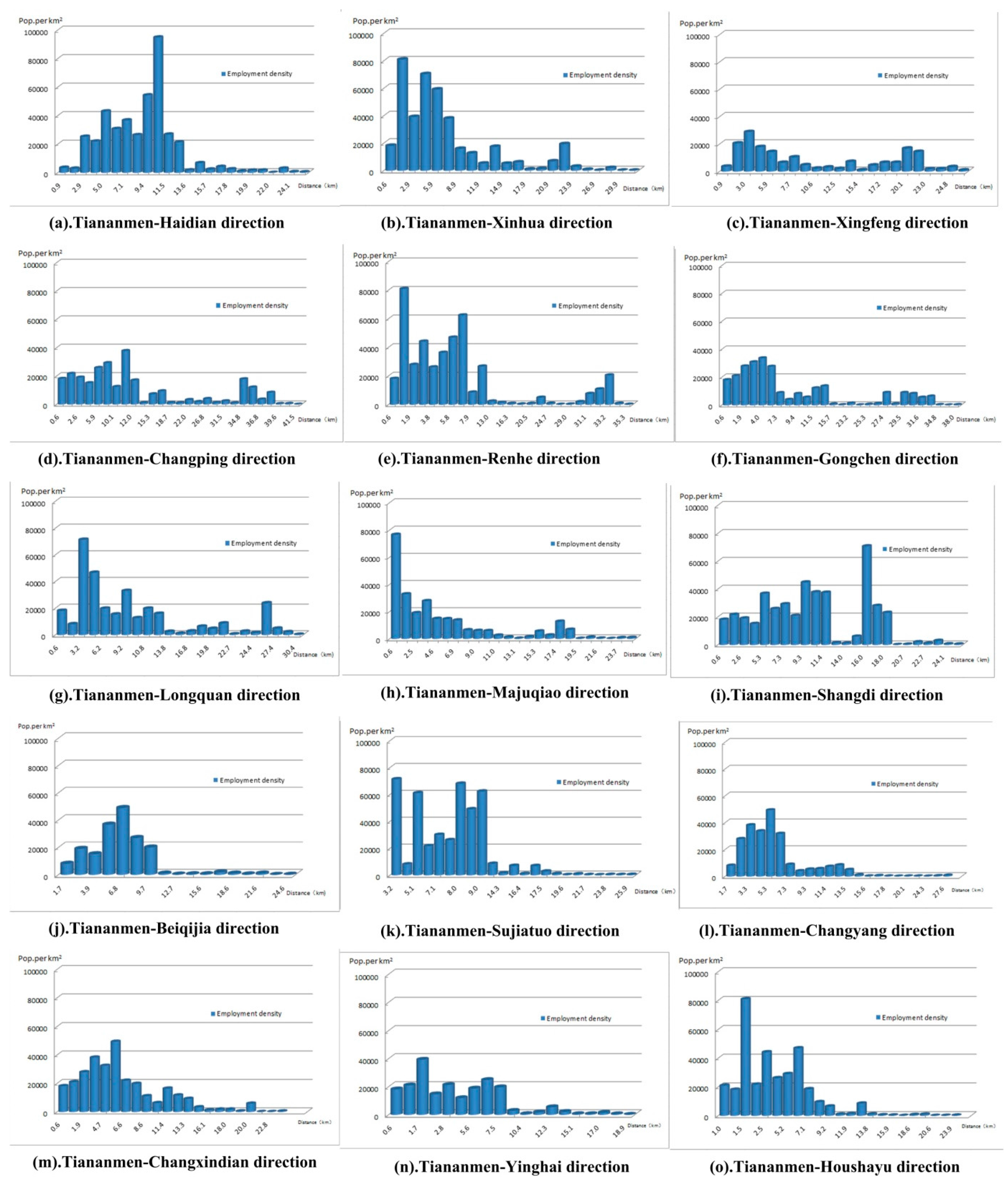
3.4. Employment Density Varies by Direction

We also examined directional variation in employment density (Figure 6). We select nine directions with potential employment subcenters, as well as six directions with no specific high-employment unit in the suburbs [52] and choose grids intercepted with each direction to draw the employment density profile for each direction (Figure 7).
Figure 6. Directions of employment density profile.
Sustainability 07 11632 g006
We can make several observations based on Figure 7. First, employment density seems to decline differently along different headings. Second, despite the overall downward trend from the center to the suburbs, in most directions, the employment density first increases and then decreases. Third, the employment density increases again in the remote suburbs in several directions, suggesting the existence of employment subcenters. Fourth, in some directions, the employment density drops very dramatically beyond a certain distance to the city center, producing a cliff-shaped profile. This suggests that employment may gather within a certain area.
These observations suggest that the spatial structure of employment shows both monocentric and polycentric characteristics. Employment density decreases from about 30,000 employees/km2 within the 3rd Ring Road to 563 employees/km2 in the outermost ring zone, suggesting a monocentric structure. At the same time, peaks of employment density in certain suburban areas suggest a polycentric pattern. We investigate this further in the next section.
Figure 7. Directional profiles of employment density.
Sustainability 07 11632 g007

4. Identification of Employment Subcenters

4.1. Results from the Monocentric Model

Table 7 reports the results of model Equation (2). The estimation adopts White’s [53] method to calculate standard errors and the covariance matrix to eliminate a potential heteroscedasticity problem.
Table 7. Regression result of the monocentric model.
Dependent Variable: ln (Employment Density)Research AreaWithin the 6th Ring RoadWithin the 5th Ring RoadWithin the 4th Ring RoadWithin the 3rd Ring Road
Constant9.552 ***10.391 ***11.486 ***10.695 ***10.392 ***
(83.04)(60.05)(61.45)(66.87)(49.60)
s−0.146 ***−0.391 ***−0.269 ***−0.123 ***−0.043
(−29.83)(20.87)(−14.86)(−4.91)(−1.02)
Adjusted R20.3330.3490.4500.1310.005
F-test803.21610.42220.7222.151.36
Sample number161181127314172
*** denotes 1% significance level; t-values are in parentheses. Samples excluded the irregularly-shaped units on the edge of the research area and the units where Tiananmen is located.
We find that both the model and the coefficient of the distance to Tiananmen are statistically significant at the 99% confidence level (Table 7). For every kilometer that the distance to Tiananmen increases, employment density decreases by 14.6%. The adjusted R2 is 0.333, indicating that this single distance variable explains 33.3% of the variation in employment density. In other words, the monocentric model works well [54] and the distance to Tiananmen is significant in explaining employment distribution in the research area.
While the monocentric model is useful in identifying employment subcenters, we wanted to clarify the scope at which it works. Accordingly, we varied the limits of the research area (Table 7). When limiting it to within the 6th Ring Road and the 5th Ring Road, the monocentric model is significant; when limiting it to within the 4th Ring Road, the monocentric model is still significant, but the explanatory power is greatly reduced; when limiting it to within the 3rd Ring Road, the monocentric model is no longer significant (Table 7). This is consistent with the direct observation from Figure 5 that, within the 3rd Ring Road and even within the 4th Ring Road, employment density is much higher, with no apparent decline away from the center. Furthermore, the explanatory power of the monocentric model is strongest within the 5th Ring Road and declines as the research area expands, which may be a result of employment subcenters in the suburbs.

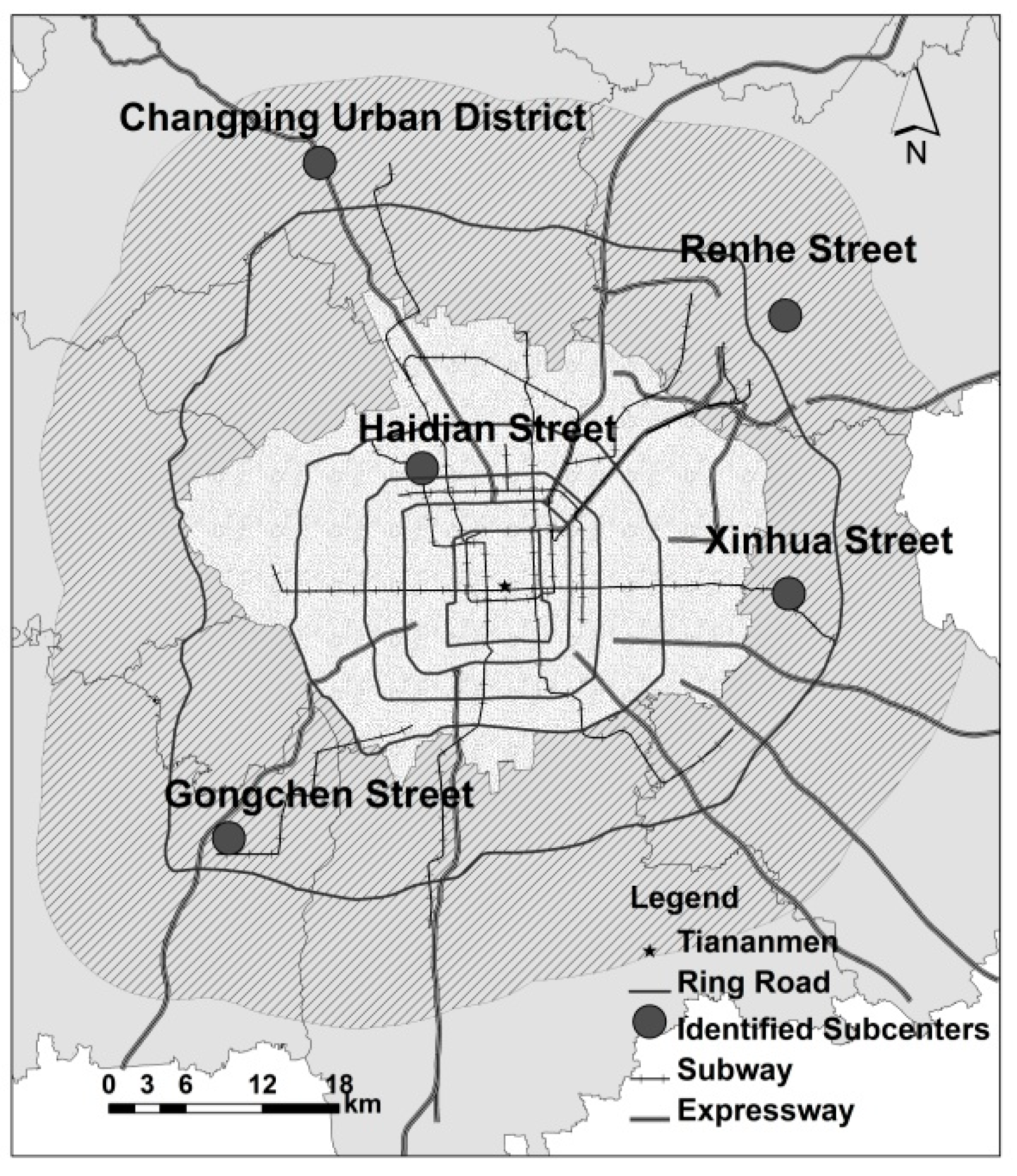
4.2. Subcenter Identification

Based on the monocentric model, we conducted a residual analysis and identified 31 research units where the residual is significantly greater than zero (at the 95% confidence level) as employment subcenter candidates. Seven of them have lower employment density than the overall average and are removed from consideration [55]. For the remaining 24 units, when the units are very close to each other (within 3 km [56]), we selected the unit with the highest employment density to represent them. This gave us nine potential sub-centers located in Shangdi Street, Haidian Street, Shahe Town, Changping Urban District (including South Street and North Street), Renhe Street, Gongchen Street, Xinhua Street, Zhangjiawan Town and Longquan Street. We use the names of these streets and towns to name the nine potential subcenters in the following discussion.

4.2.1. Effects of Potential Employment Subcenters on Overall Employment Density

The results of model Equation (4) are shown on the left side of Table 8. After some tests, we include two dummy variables of the distance to the subway station and highway and one continuous variable of the distance to the airport into the regression function to control other factors’ influences. The distances to Tiananmen, Haidian Street, Changping Urban District, Renhe Street and Gongchen Street have a significant impact on employment density. The distances to Shangdi Streets, Longquan Street and Xinhua Street are also significant, but the coefficient signs are positive, which is not consistent with the expectations. One possible problem of this is collinearity. For example, Shangdi Street, Haidian Street and Shahe Street are in the same direction, and the distance between them is short, so the distances to these three potential subcenters are highly correlated [57]. Another reason is that the effect of proximity to a subcenter declines rapidly with distance, as mentioned in Section 2.3.2.
Table 8. Regression results of potential subcenter test.
Dependent Variable in (Employment Density)Model Equation (4) (Distances to Subcenters)Dependent Variable in (Employment Density)Model Equation (5) (Inverse Distances to Subcenters)
Constant9.086 ***Constant7.136 ***
(7.01) (29.01)
s−0.172 ***S−0.111 ***
(−7.45) (−11.85)
s Haidian Street−0.265 ***1/s Haidian Street3.469 ***
(−4.61) (4.21)
s Shangdi Street0.302 ***1/s Shangdi Street0.568
(4.32) (0.65)
s Longquan Street0.089 ***1/s Longquan Street1.722
(4.72) (1.56)
s Xinhua Street0.065 **1/s Xinhua Street1.716 ***
(2.15) (2.86)
s Renhe Street−0.101 ***1/s Renhe Street6.111 ***
(−5.89) (5.63)
s Changping Urban District−0.073 ***1/s Changping Urban District6.821 ***
(−3.24) (7.42)
s Shahe Town0.0191/s Shahe Town−0.871
(0.35) (−0.95)
s Zhangjiawan Street0.0191/s Zhangjiawan Street1.462
(0.78) (1.62)
s Gongchen Street−0.063 ***1/s Gongchen Street4.735 ***
(−3.45) (5.63)
x Airport0.088 ***x Airport0.054
0–1 km from subway station1.389 ***0–1 km from subway station1.783 ***
(7.67) (10.01)
1–3 km from subway station0.835 ***1–3 km from subway station0.828 ***
(5.62) (5.35)
0–1 km from the highway0.362 ***0–1 km from the highway0.331 ***
(2.91) (2.64)
1–3 km from the highway0.1341–3 km from the highway0.037
(1.08) (0.312)
Adjusted R20.441Adjusted R20.437
F-test83.35F-test82.03
Sample number1062Sample number1062
*** and ** denote the 1% and 5% significance level, respectively; t-values are in parentheses.
To solve these problems, model Equation (5) has been estimated, and the result is shown in Table 8 on the right. The inverse of the distance between a grid cell and Haidian Street, Xinhua Street, Renhe Street, Changping Urban District and Gongchen Street is significant, and the effects are positive, as expected. However, the inverse distances to Shangdi Street, Longquan Street, Shahe Town and Zhangjiawan Street are not significant. These results suggest that Haidian Street, Xinhua Street, Renhe Street, Changping Urban District and Gongchen Street are more likely to be employment subcenters.

4.2.2. Effects of Potential Subcenters on Local Employment Density

The results demonstrate that most models are significant at the 95% confidence level, with a few exceptions, including the models within 5 km of Renhe Street and Shahe Town and models within 5 km and 10 km of Zhangjiawan Town (Table 9). All coefficient signs of the subcenters are as expected.
Each of the five subcenters identified in Section 4.2.1 has a strong influence on local employment density within certain distances. Changping Urban District and Xinhua Street significantly affect employment density within a radius of 5 km, 10 km and 15 km. Haidian Street and Gongchen Street are significant within a radius of 5 km and 10 km, but their influence is unclear when the radius is expanded to 15 km. Renhe Street is somewhat unique, given that its effects are significant at 10 km and 15 km, but not significant within a radius of 5 km. It could be that employment density does not decline significantly within 5 km of Renhe Street. For the other potential subcenters, Shangdi Street and Longquan Street influence employment density within a radius of 5–10 km, while Shahe Town and Zhangjiawan Street have little effect on local employment density.
According to these results, the nine potential employment subcenters can be divided into three types. The first includes Haidian Street, Xinhua Street, Changping Urban District, Gongchen Street and Renhe Street. These five candidates clearly influence local and overall employment distribution. The second type includes Shangdi Street and Longquan Street, which influence only local employment distribution. The third type includes Shahe Town and Zhangjiawan Street, which have high employment density, but little effect on employment distribution. According to McMillen [28], a subcenter should have a significant effect on overall employment. We therefore identify the first group of candidates as Beijing’s employment subcenters (Figure 8).
Table 9. Local regression results of employment subcenters.
Dependent Variable5 km10 km15 km5 km10 km15 km5 km10 km15 km
Haidian StreetChangping Urban DistrictRenhe Street
Constant9.750 ***12.911 ***11.844 ***5.1879.453 ***9.682 ***12.946 ***9.971 ***10.548 ***
(−71.49)(30.12)(40.83)(1.67)(7.72)(10.29)(3.52)(9.03)(9.39)
S−0.480 ***−0.289 ***−0.244 ***0.119−0.062−0.095 ***−0.195−0.089 **−0.106 ***
(−17.63)(−12.11)(−18.3)(1.36)(−1.96)(−4.13)(−1.83)(−2.04)(−3.59)
s subcenters−0.301 **−0.124 **−0.038−0.206 ***−0.300 ***−0.146 ***−0.026−0.215 ***−0.213 ***
(−2.1)(−2.54)(−1.83)(−4.30)(−5.06)(−4.21)(−0.11)(−2.90)(−4.86)
Adjusted R20.6640.5360.5510.340.180.090.0420.0790.126
F35.6381.19186.559.8313.2811.361.705.0413.68
Sample number37141355341162033496177
Gongchen StreetXinhua StreetLongquan Street
Constant3.5817.558 ***7.579 ***10.558 ***9.097 ***9.527 ***18.405 ***11.98 ***10.79 ***
(1.14)(7.11)(10.36)(3.97)(10.79)(18.27)(4.18)(10.25)(12.70)
S−0.157−0.022−0.072 ***−0.051−0.062 **−0.127 ***−0.335−0.209 ***−0.204 ***
(−1.42)(−0.65)(−4.53)(−0.46)(−2.00)(−7.90)(−1.89)(−4.52)(−8.93)
s subcenter−0.559 **−0.231 ***−0.016−0.730 ***−0.238 ***−0.074 **−1.097 ***−0.256 ***−0.038
(−2.29)(−3.18)(−0.48)(−2.71)(−3.61)(−2.38)(−2.83)(−2.72)(−0.82)
Adjusted R20.1130.0680.0650.1450.1030.1880.3380.2120.261
F-test2.995.5110.363.808.5631.026.6412.9032.24
Sample number33125270351322603099184
Shangdi StreetShahe TownZhangjiawan Town
Constant12.650 ***12.346 ***11.490 ***9.945 ***8.854 ***8.10 ***7.2408.862 ***10.599 ***
(8.28)(21.13)(35.16)(3.63)(11.49)(18.74)(1.78)(3.77)(7.71)
S−0.230−0.265 ***−0.234 ***−0.157−0.123 ***−0.085 ***−0.040−0.103−0.155 ***
(−1.41)(−9.96)(−18.73)(−1.56)(−4.79)(−6.82)(−0.32)(−1.51)(−3.89)
s-subcenter−0.295 **−0.069−0.018−0.044−0.0360.006−0.086−0.066−0.102
(−2.56)(−1.23)(−0.74)(−0.02)(−0.64)(−0.82)(−0.32)(−0.66)(−1.92)
Adjusted R20.190.4220.550.0130.1350.1320.0070.0280.080
F-test4.9851.29179.211.2211.5323.241.121.197.71
Sample number37140293351362922961156
*** and ** denote the 1% and 5% significance level, respectively; t-values are in parentheses.
Figure 8. Beijing’s confirmed employment subcenters.
Sustainability 07 11632 g008

4.3. Polycentric Model

Based on the five identified subcenters, we use model Equation (5) to explain the overall employment density distribution. The regression results are shown in Table 10. To compare the polycentric and monocentric models, a monocentric model with added control variables has also been conducted here.
The polycentric model and the coefficients of all independent variables are significant at a 99% confidence level. A partial F-test suggests that the five subcenter distance variables together are significantly more than zero, indicating that these identified subcenters influence the overall employment distribution. However, adding the distance to the five subcenters improves the entire model’s explanatory power by only four percent: the adjusted R2 of the polycentric model is 0.434, compared to the monocentric model’s adjusted R2 of 0.393.
Table 10. Comparison of the monocentric and polycentric models.
Dependent Variable (Employment Density)Monocentric Model (Add Control Variables)Polycentric Model
Constant7.660 ***7.176 ***
(33.53)(30.49)
S−0.096 ***−0.112 ***
(−11.67)(−12.46)
1/s Haidian Street 2.953 ***
(4.17)
1/s Changping Urban District 5.904 ***
(7. 28)
1/s Xinhua Street 2.002 ***
(2.71)
1/s Renhe Street 6.601 ***
(5.82)
1/s Gongchen street 4.693 ***
(5.68)
x Airport0.0690.096
(1.17)(1.34)
0–1 km from subway station2.009 ***1.760 ***
(11.53)(10.07)
1–3 km from subway station0.896 ***0.779 ***
(5.95)(5.38)
0–1 km from the highway0.560 ***0.373 ***
(4.04)(3.03)
1–3 km from the highway0.1520.013
(1.26)(0.29)
Adjusted R20.3930.434
F-test174.29110.98
Sample number16021602
*** denotes the 1% significance level; t-values are in parentheses.

5. Discussion and Conclusions

Although many cities in developed countries have polycentric or even dispersed employment patterns [41,58,59,60,61,62], the situation in Beijing appears to be different. First, the city still has very strong monocentric characteristics. The single factor of a cell’s distance to Tiananmen explains 33.3% of its employment density, a figure that increases further when peripheral cells are excluded (34.9% inside the 6th Ring Road, 45.0% inside the 5th Ring Road). Second, the city has a very large employment center, which is centered at Tiananmen and generally overlaps with the 4th Ring Road. We call this center “large” because it has an area of about 300 km2 (6.8% of the research area) and accounts for 58.7% of employment, whereas other cities’ downtown areas can often be treated as points. Third, despite the identification of five sub-centers, it is difficult to conclude that the city has achieved a polycentric structure, as the polycentric model improves the explanatory power of the overall employment distribution by only 4% over the monocentric one [63,64]. Based on these findings, we conclude that the spatial structure of Beijing is still monocentric, but may be in transition to a polycentric pattern.
Beijing has tried to foster subcenters and to achieve a decentralized spatial development pattern to a certain degree; however, our study suggests that the success of these efforts has been limited. The monocentric model still explains the spatial structure of the city’s employment very well, and adding the identified subcenters improves its explanatory power by only four percentage points. At the same time, though four of the five identified subcenters—Xinhua Street, Changping Urban District, Gongchen Street and Renhe Street—are located in the planned new towns, the other three new suburb towns have not achieved development as expected. We speculate that several factors contribute to Beijing’s strongly monocentric character and the formation of its large employment center. First, the central city enjoys better infrastructure than other areas and hosts most of the central and city government departments, schools, hospitals, museums, public facilities and parks. Second, the ring-and-radials road structure plays a very important role in facilitating the concentration of people and economic activities in the central city. Third, and more important, the power of agglomeration remains decisive. As a result, new development still prefers locations close to the central city.
With these somewhat disappointing results in mind, several inferences may be drawn from the findings of this study. First, the monocentric characteristics of employment distribution suggest that the agglomeration economy still plays a dominate role in Beijing, and so planning interventions and heavy public investment in decentralized development may result in a loss of economic efficiency [65]. We feel that planning tools are useful in guiding and regulating development, but market needs and the efficiency of public investment also deserve careful considerations. Given the fact that the city center still accommodates most of the employment, the government should also pay attention to further improving the infrastructure and facilities of existing developed areas, thus making the city a more attractive and livable place. Second, given that the employment is still concentrated in the city center based on the findings of this paper while the population has already redistributed to the suburban area according to the literature suggests the possibility of a more imbalanced job-housing spatial distribution and longer commuting distances, which also deserves more attention when making plans and policies.

Acknowledgments

This research is supported by “the Fundamental Research Funds for the Central Universities”. The authors gratefully thank the reviewers and the editor. We also thank Matt Turner, A-xing Zhu in the Department of Geography University of Wisconsin-Madison for their additional guidance, and we acknowledge the help provided by Haoran Jin, Xin Yao, Yuncheng Huang, Pingping Ma, Xin Tan and Xiaoqing Yang in the School of Geography Beijing Normal University for their constructive suggestions for this paper. Thanks also to Jacob Fleming for his language polishing and editing.

Author Contributions

Daquan Huang developed the original idea and contributed to the research design, writing and modification. Zhen Liu was responsible for data collection and processing, writing and modification. Xingshuo Zhao contributed to the research design, writing, modification and provided guidance. All authors have read and approved the final manuscript. The authors are very grateful to the anonymous referees and the editors for their helpful comments on an earlier version of this paper.

Conflicts of Interest

The authors declare no conflict of interest.

References and Notes

  1. Bai, X.M.; Shi, P.J.; Liu, Y.S. Realizing China’s urban dream. Nature 2014, 509, 158–160. [Google Scholar] [CrossRef] [PubMed]
  2. Hu, Z. Review and outlook of Population Scale in Beijing. Urban Stud. 2011, 18, 8–10. (In Chinese) [Google Scholar]
  3. Hu, Z. Review and Recognition on Urban Size of Beijing. J. Urban Reg. Plan. 2011, 2, 1–18. (In Chinese) [Google Scholar]
  4. Huang, D.; Jin, H.; Zhao, X.; Liu, S. Factors Influencing the Conversion of Arable Land to Urban Use and Policy Implications in Beijing, China. Sustainability 2015, 7, 180–194. [Google Scholar] [CrossRef]
  5. Sun, C.; Zheng, S.Q.; Wang, R. Restricting driving for better traffic and clearer skies: Did it work in Beijing? Transp. Policy 2014, 32, 34–41. [Google Scholar] [CrossRef]
  6. Wen, H.; Sun, J.; Zhang, X. Study on Traffic Congestion Patterns of Large City in China Taking Beijing as an Example. Procedia-Soc. Behav. Sci. 2014, 138, 482–491. [Google Scholar] [CrossRef]
  7. Cai, H.; Xie, S.D. Traffic-related air pollution modeling during the 2008 Beijing Olympic Games: The effects of an odd-even day traffic restriction scheme. Sci. Total Environ. 2011, 409, 1935–1948. [Google Scholar] [CrossRef] [PubMed]
  8. Hou, L.F.; Wang, S.; Dou, C.; Zhang, X.; Yu, Y.; Zheng, Y.N.; Avula, U.; Hoxha, M.; Diaz, A.; McCracken, J.; et al. Air pollution exposure and telomere length in highly exposed subjects in Beijing, China: A repeated-measure study. Environ. Int. 2012, 48, 71–77. [Google Scholar] [CrossRef] [PubMed]
  9. Tian, L.; Zhang, W.; Lin, Z.Q.; Zhang, H.S.; Xi, Z.G.; Chen, J.H.; Wang, W. Impact of Traffic Emissions on Local Air Quality and the Potential Toxicity of Traffic-related Particulates in Beijing, China. Biomed. Environ. Sci. 2012, 25, 663–671. [Google Scholar] [PubMed]
  10. Dang, Y.; Liu, Z.; Zhang, W. Land-based interests and the spatial distribution of affordable housing development: The case of Beijing, China. Habitat Int. 2014, 44, 137–145. [Google Scholar] [CrossRef]
  11. Yu, L.; Cai, H.P. Challenges for housing rural-to-urban migrants in Beijing. Habitat Int. 2013, 40, 268–277. [Google Scholar] [CrossRef]
  12. The urban planning aims to evacuate both the employment and population from the central city. For employment, the government, on one hand, encourages industries move to the suburb; on the other hand, it sets up many development zones in the suburb. For population, many residential communities have been built with the boom of the real estate in the suburb.
  13. Huang, D.Q.; Wan, W.; Dai, T.Q.; Liang, J.S. Assessment of industrial land use intensity: A case study of Beijing economic-technological development area. Chin. Geogr. Sci. 2011, 21, 222–229. [Google Scholar] [CrossRef]
  14. Dong, G. Sixty years and twenty years—Review and Prospect of the modernization development process in Beijing (2). Beijing Plan. Rev. 2010, 5, 168–171. (In Chinese) [Google Scholar]
  15. Dong, G. Sixty years and twenty years—Review and Prospect of the modernization development process in Beijing (1). Beijing Plan. Rev. 2010, 6, 177–180. (In Chinese) [Google Scholar]
  16. Kuang, W.; Liu, J.; Shao, Q.; Sun, C. Spatio-temporal patterns and driving forces of urban expansion in Beijing Central City since 1932. J. Geo-Inf. Sci. 2009, 4, 428–435. (In Chinese) [Google Scholar] [CrossRef]
  17. Beijing is composed of fourteen districts and two counties. The central city covers all of Xicheng District and Dongcheng District and part of Haidian District, Chaoyang District, Fengtai District, and Shijingshan District. Nine of the ten other suburban districts and counties have one new town each. Daxing district has two new towns: Huangcun new town, where Daxing district government is located, and Yizhuang new town, where Beijing Economic-Technological Development Area is located.
  18. Feng, J.; Zhou, Y. The Growth and Distribution of Population in Beijing Metropolitan Area (1982–2000). Acta Geogr. Sinica 2003, 58, 903–916. (In Chinese) [Google Scholar]
  19. Feng, J.; Zhou, Y. The social spatial structure of Beijing Metropolitan Area and its evolution: 1982–2000. Geogr. Res. 2003, 22, 465–483. (In Chinese) [Google Scholar]
  20. Feng, J.; Zhou, Y.; Wu, F. New trends of suburbanization in Beijing since 1990: From government-led to market-oriented. Reg. Stud. 2008, 42, 83–99. [Google Scholar] [CrossRef]
  21. Feng, J.; Wang, F.; Zhou, Y. The spatial restructuring of population in metropolitan Beijing: Toward polycentricity in the post-reform era. Urban Geogr. 2009, 30, 779–802. [Google Scholar] [CrossRef]
  22. Ma, Q.; Zhang, W. Characteristics and factors analyses of suburbanization in Beijing. Geogr. Res. 2006, 25, 121–130. (In Chinese) [Google Scholar]
  23. Wang, F.; Zhou, Y. Modelling urban population densities in Beijing 1982–1990: Suburbanisation and its causes. Urban Stud. 1999, 36, 271–287. [Google Scholar] [CrossRef]
  24. Alonso, W. Location and land use: Toward a general theory of land rent. Econ. Geogr. 1964, 42, 277–279. [Google Scholar]
  25. Brueckner, J.K. The structure of urban equilibria: A unified treatment of the Muth-Mills model. Handb. Reg. Urban Econ. 1987, 2, 821–845. [Google Scholar]
  26. Mills, E.S. An aggregative model of resource allocation in a metropolitan area. Am. Econ. Rev. 1967, 57, 197–210. [Google Scholar]
  27. Muth, R. Cities and Housing: The Spatial Patterns of Urban Residential Land Use; University of Chicago Press: Chicago, IL, USA, 1969. [Google Scholar]
  28. McMillen, D.P. Nonparametric employment subcenter identification. J. Urban Econ. 2001, 50, 448–473. [Google Scholar] [CrossRef]
  29. Tao, R.; Jin, Y. Improvement of Data Quality Assessment of Economic Census in China. Stat. Res. 2009, 26, 8–12. (In Chinese) [Google Scholar]
  30. Gu, Y.; Zheng, S.; Cao, Y. The Identification of Employment Centers in Beijing. Urban Stud. 2009, 9, 118–124. (In Chinese) [Google Scholar]
  31. Liu, X.; Sun, T.; Li, G. Research on the spatial structure of employment distribution in Beijing. Geogr. Res. 2011, 30, 1262–1270. (In Chinese) [Google Scholar]
  32. Sun, T.; Wang, L.; Li, G. Distributions of Population and Employment and Evolution of Spatial Structures in the Beijing Metropolitan Area. Acta Geogr. Sinica 2012, 67, 829–840. (In Chinese) [Google Scholar]
  33. Beijing has three levels of governments: The municipality, the district or county, and the town (township or street). The average area of towns (townships or streets) in Beijing is about 22 km2.
  34. The First Ring is actually the walls of the Forbidden City.
  35. Long, Y.; Zhang, Y.; Cui, C. Identifying Commuting Pattern of Beijing Using Bus Smart Card Data. Acta Geogr. Sin. 2012, 67, 1339–1352. (In Chinese) [Google Scholar]
  36. There are eleven new towns in all, but four of them are remote from the central city, averaging more than 65 km from the city center (Tiananmen)
  37. In matching the enterprise locations, “Exact matching” accounts for 79.3% and “Non-exact matching” accounts for 20.7%. It can be hard or impossible to match a company with a building exactly for two reasons. First, large companies can have multiple buildings, requiring us to use their geometrical center as the company’s geographic coordinate. Second, some company addresses—for example, No.19 XX Street—are not sufficiently detailed to allow us to specify an exact match. These cases lead to some errors, but these are acceptable given the size of the research unit (1.5 km × 1.5 km).
  38. Beijing Municipal Statistical Bureau. Beijing Statistical Yearbook 2011; China Statistics Press: Beijing, China, 2011.
  39. The 560 companies that were eliminated from our dataset were selected in two ways. First, some companies were identified as not limited to Beijing by their names, such as XX headquarters. Second, for companies with more than 3000 employees, we conducted internet searches on the distribution of their activities. If we found, for example, that the company has branches or factories in many locations, we eliminated it from our data.
  40. McMillen, D.P.; Lester, T.W. Evolving subcenters: Employment and population densities in Chicago, 1970–2020. J. Hous. Econ. 2003, 12, 60–81. [Google Scholar] [CrossRef]
  41. McDonald, J.F.; Prather, P.J. Suburban employment centres: The case of Chicago. Urban Stud. 1994, 31, 201–218. [Google Scholar] [CrossRef]
  42. Giuliano, G.; Small, K.A. Subcenters in the Los Angeles region. Reg. Sci. Urban Econ. 1991, 21, 163–182. [Google Scholar] [CrossRef]
  43. As more than a quarter of the towns (townships, streets) and other potential employment subcenters are smaller than 4 km2, the grid should be smaller than 4 km2.
  44. McMillen, D.P.; McDonald, J.F. Suburban subcenters and employment density in metropolitan Chicago. J. Urban Econ. 1998, 43, 157–180. [Google Scholar] [CrossRef]
  45. McDonald, J.F. The identification of urban employment subcenters. J. Urban Econ. 1987, 21, 242–258. [Google Scholar] [CrossRef]
  46. McDonald, J.F.; McMillen, D.P. Employment subcenters and land values in a polycentric urban area: The case of Chicago. Environ. Plan. A 1990, 22, 1561–1574. [Google Scholar] [CrossRef]
  47. Small, K.A.; Song, S.F. Population and employment densities—Structure and change. J. Urban Econ. 1994, 36, 292–313. [Google Scholar] [CrossRef]
  48. Employment density around Tiananmen is very low, but we still can regard it as the center. First, it is the city center in city planning. The Beijing government has always taken Tiananmen as the center to design the layout of the city. Second, its scope is so small that we can regard it as a point. Third, many studies have taken Tiananmen as the center to investigate the distribution of population and employment [21,31,32].
  49. Muñiz, I.; Garcia-López, M.À.; Galindo, A. The effect of employment sub-centres on population density in Barcelona. Urban Stud. 2008, 45, 627–649. [Google Scholar] [CrossRef]
  50. Heikkila, E.; Gordon, P.; Kim, J.I.; Peiser, R.B.; Richardson, H.W.; Dale-Johnson, D. What happened to the CBD-distance gradient? Land values in a policentric city. Environ. Plan. A 1989, 21, 221–232. [Google Scholar] [CrossRef]
  51. For example, the Xinhua Street which is the main part of Tongzhou new town specialized in comprehensive service, the Renhe Street which is the main part of Shunyi new town specialized in aviation logistics, the Gongchen Street which is the main part of Fangshan new town specialized in new materials industry, and the Changping urban district which is the main part of Changping new town specialized in research and development. Their developing directions have also different in the planning to undertake different functions of Beijing.
  52. The nine directions are Tianmen-Haidian, Tianmen-Xinhua, Tianmen-Xingfeng, Tianmen-Changping, Tianmen-Renhe, Tianmen-Gongchen, Tianmen-Longquan, Tianmen-Majuqiao and Tianmen-Shangdi.
  53. White, H. A heteroskedasticity-consistent covariance matrix estimator and a direct test for heteroskedasticity. Econometrica 1980, 48, 817–838. [Google Scholar] [CrossRef]
  54. McDonald [41] adopted seven forms of monocentric models to test the employment distribution of Chicago .The adjusted R2 is between 0.258 and 0.336 while the negative exponential model is 0.296. Small et al. [47] used the negative exponential model to examine the employment distribution in Los Angeles region. The adjusted R2 is 0.395 in 1970 and 0.388 in 1980.
  55. All seven of these are located in remote suburban districts, including four in Fangshan District and three in Shunyi District.
  56. The selection of a 3 km boundary is somewhat subjective. Related research has no strict definition of adjacency. McMillen et al. [40] defined it as within 1.5 miles. Giuliano et al. [42] defined it as at least 0.25 miles from a common border. Here we referred to the definition of McMillen et al. [40], and with an eye toward the size of our study unit, selected 3 km as constituting adjacency.
  57. The distance between Shangdi street and Haidian street is about 7 km and the correlation coefficient is 0.91. The distance between Shangdi street and Shahe street is about 8 km and the correlation coefficient is 0.93. The distance between Haidian street and Shahe street is about 13 km and the correlation coefficient is 0.76.
  58. Cervero, R.; Wu, K.L. Polycentrism, commuting, and residential location in the San Francisco Bay Area. Environ. Plan. A 1997, 29, 865–886. [Google Scholar] [CrossRef] [PubMed]
  59. Glaeser, E.L.; Kahn, M.E. Decentralized Employment and the Transformation of the American City. National Bureau of Economic Research, 2011. Availiable online: http://www.nber.org/papers/w8117 (accessed on 17 August 2015).
  60. Garcia-López, M.-À.; Muñiz, I. Employment decentralisation: Polycentricity or scatteration? The case of Barcelona. Urban Stud. 2010. [Google Scholar] [CrossRef]
  61. Hughes, H.L. Metropolitan structure and the suburban hierarchy. Am. Sociol. Rev. 1993, 58, 417–433. [Google Scholar] [CrossRef]
  62. Veneri, P. The identification of sub-centres in two Italian metropolitan areas: A functional approach. Cities 2013, 31, 177–185. [Google Scholar] [CrossRef]
  63. Compared with monocentric model, the explanatory power of the polycentric model has a significant improvement in the research of Small et al. [47] and Wang et al. [64].
  64. Wang, F.; Meng, Y. Analyzing urban population change patterns in Shenyang, China 1982–1990: Density function and spatial association approaches. Geogr. Inf. Sci. 1999, 5, 121–130. [Google Scholar]
  65. Ding, C.; Bethka, K. Employment Concentration and Urban Economic Growth. Urban Plan. Overseas 2005, 4, 11–18. (In Chinese) [Google Scholar]

