Experiential Knowledge Complements an LCA-Based Decision Support Framework

Abstract

A shrimp farmer in Taiwan practices innovation through trial-and-error for better income and a better environment, but such farmer-based innovation sometimes fails because the biological mechanism is unclear. Systematic field experimentation and laboratory research are often too costly, and simulating ground conditions is often too challenging. To solve this dilemma, we propose a decision support framework that explicitly utilizes farmer experiential knowledge through a participatory approach to alternatively estimate prospective change in shrimp farming productivity, and to co-design options for improvement. Data obtained from the farmer enable us to quantitatively analyze the production cost and greenhouse gas (GHG) emission with a life cycle assessment (LCA) methodology. We used semi-quantitative graphical representations of indifference curves and mixing triangles to compare and show better options for the farmer. Our results empower the farmer to make decisions more systematically and reliably based on the frequency of heterotrophic bacteria application and the revision of feed input. We argue that experiential knowledge may be less accurate due to its dependence on varying levels of farmer experience, but this knowledge is a reasonable alternative for immediate decision-making. More importantly, our developed framework advances the scope of LCA application to support practically important yet scientifically uncertain cases.

1. Introduction

Farmer-based innovation will boost agricultural (including aquaculture) yield and protect the planet [1], but it is often neglected in terms of research and investment [1,2]. In contrast to a one-size-fits-all global-scale improvement (the Green Revolution), agricultural innovation relies on farmer expertise on the local environment and traditional wisdom of practice [3]. MacMillan and Benton [1] argue that the effect of conventional institutional effort is slowing down based on recent global production. Thus, engaging farmers in research is the next stage for improvement. According to the Food and Agriculture Organization of the United Nations, individuals or single families run 90% of the farms around the world [4]. Among the small-scale farmers, those in poor or developing regions can still increase their productivity given sufficient support [5]. The potential of farmer-based innovation is agreed upon, but progress can be slow and random. Therefore, a decision support framework from the scientific community that is designed for empowering farmers can promote sustainable agriculture [1].

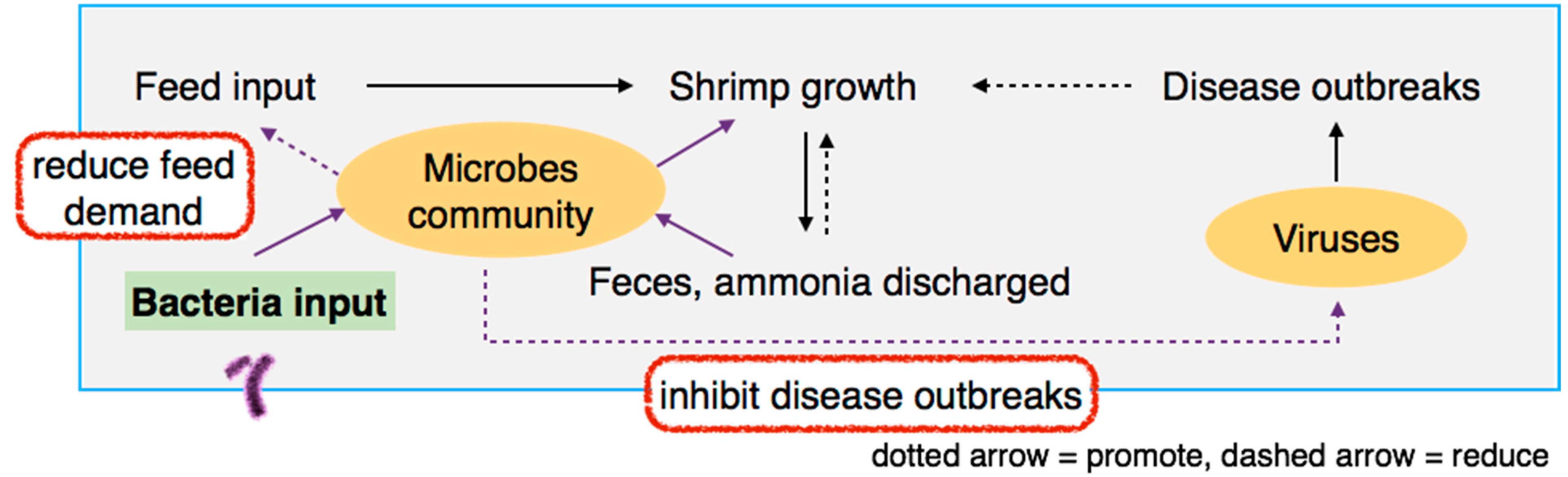
This research aims at exploring farmer-based innovation using a case of shrimp farming. Generally, innovative methods for improving shrimp farming productivity are uncertain due to the complex mechanisms in biological growth and ecology [6,7]. Rong-Hong Yan, a Taiwanese shrimp farmer, has innovated a unique ecological method (or innovation) that improves pond ecology by regularly applying specific types of heterotrophic bacteria, i.e., Bacillus spp., with a revised feeding strategy (Figure 1). In the shrimp pond, the bacteria are able to grow to a significant number by feeding on existing nutrients and shrimp metabolic waste. The bacteria reduce shrimp disease outbreaks by interfering with the virus activity, the main cause of unstable shrimp production [8,9,10]. Furthermore, the bacteria can reduce feed demand by serving as an alternative organic food source. The innovation has proved effective according to the farmer’s trial and error. In other words, no direct scientific knowledge to quantify the effects of the method has been applied. Moreover, the earthen pond exhibits specific micro-ecology, soil carbon, pH, and other environmental characteristics. These variations imply that the optimum practice of feeding and the bacteria application cannot be standardized as an across-the-board measure. Despite the uncertainty, the farmer must decide the amount of feed and bacteria application each time based on experiential knowledge in the hope of achieving a better investment return and a lower GWP. Therefore, we are seeking a reusable decision support framework to strategize how often the bacteria should be applied and how much feed input can be revised.

Conventional experimental approaches that require rigorous examination are ineffective for the following reasons: (1) actual ground conditions are difficult to simulate in the laboratory; (2) real-time monitoring of the shrimp growth effect in turbid water is difficult; (3) general conclusions cannot be drawn from a one-pond experiment as each pond is environmentally and ecologically unique; (4) small-scale household farmers cannot afford to risk the entire farming cycle for an experiment due to the limited number of ponds and options for alternative income.

Figure 1. Schematic representation of the ecological shrimp farming method innovated by the farmer, showing the hypothetical effect that bacteria input has in inhibiting disease outbreak and reducing feed demand.

Figure 1. Schematic representation of the ecological shrimp farming method innovated by the farmer, showing the hypothetical effect that bacteria input has in inhibiting disease outbreak and reducing feed demand.

This research proposes a decision support framework that systematically utilizes farmer experiential knowledge when scientifically sound knowledge is insufficient. Experiential knowledge includes explicit, implicit, and tacit knowledge [11]. Implicit knowledge is hard to articulate compared to explicit knowledge, and tacit knowledge cannot be articulated. Tacit knowledge is context-specific, experience-based, often used intuitively and unconsciously, and constitutes a keen sense of skills that is challenging to replicate [3]. Unlike formal knowledge, the value of experiential knowledge is often neglected and is rarely extracted to scientific research due to its subjectivity [3]. In shrimp farming, farmers acquire an implicit ability to predict shrimp growth through observing the shapes of small sample shrimps, the number of seagulls surrounding a shrimp pond, the color and turbidity of the water, and by relying on farming experiences. Engaging farmers in research can provide invaluable insights for evaluating uncertainties in modeling the prospective change in practices. In this research, experiential knowledge is utilized in estimating shrimp yield in response to bacteria input frequency, in co-designing scenarios for feed input revision (i.e., reducing total amount, replacing animal-based protein with plant-based), and in estimating likely shrimp yield.

The developed decision support framework is built on life cycle assessment (LCA) methodology. LCA quantifies the environmental impact and production cost of providing one product or service by explaining the impact spanning across its life cycle stages [12]. This is often termed cradle-to-grave, a scope covering raw material acquisition, production, transportation, consumer use, and end-of-life disposal [13]. This system-wide view provides a holistic analysis to avoid any hasty decisions due to the ignorance of burden shift from one life cycle stage to the other. For instance, farmer-based innovation is often limited to the on-farm production stage because other stages are intangible to farmers. Constraints might alter the decision when determining the environmental friendliness of the activity. In the case of greenhouse gas (GHG) emissions, if the emissions of feed manufacturing remain unexplained, then farmers may be encouraged to apply excess amounts of feed to increase shrimp farming productivity. Technically, harvesting more shrimp means lower emissions for each unit of shrimp production, but increasing emissions in the feed manufacturing stage will cancel that effect. In fact, farming activity, as a whole, contributes significantly to global warming potential (GWP), as estimated by the International Panel on Climate Change (IPCC) [14].

Previous LCA studies fail to elucidate how to incorporate farmer experiential knowledge into a LCA-based decision support framework. A review in aquaculture [15] finds (1) more studies on non-finfish species, e.g., shrimp, production in developing regions; and (2) better farming practices are required to protect the environment. Mungkung et al. [16] investigated the Thailand shrimp farming industry to examine the application of product eco-labeling, which is designed to create consumer awareness. They examine the differences between impact characterization methods of CML2, IMPACT2002+, and Eco-indicator. Cao et al. [17] investigate the environmental impact of shrimp supply chains on the local Chinese market and the American exporting market. They assess the potential of lowering environmental impact through scenarios of various energy structures (e.g., eliminating coal power plants), feed conversion ratios, and substitution of feed protein sources. In summary, these studies support the decision-making of government policies and research projects, rather than looking into farmer needs. An exception to the above is a study that attempted to include the expectations of sugarcane farmers in decision-making [18]. For farmer-based innovation, LCA must be tailored to a transdisciplinary setting [19], where the viewpoints of non-academic actors, i.e., farmers, are factored into the solution.

This work contributes in proposing a novel LCA-based decision support framework that utilizes experiential knowledge to confront the challenges of farmer-based innovation and addresses uncertainties in estimating prospective outcomes. Two sets of easy-to-understand graphical representations, indifference curves and mixing triangles, are developed to support the farmer in the demonstrated case. Here, the role of the farmer is explored from two aspects: (1) providing experiential knowledge to supplement analysis in the absence of scientific knowledge and (2) participating in the scenario analysis as the final decision maker.

2. Materials and Methods

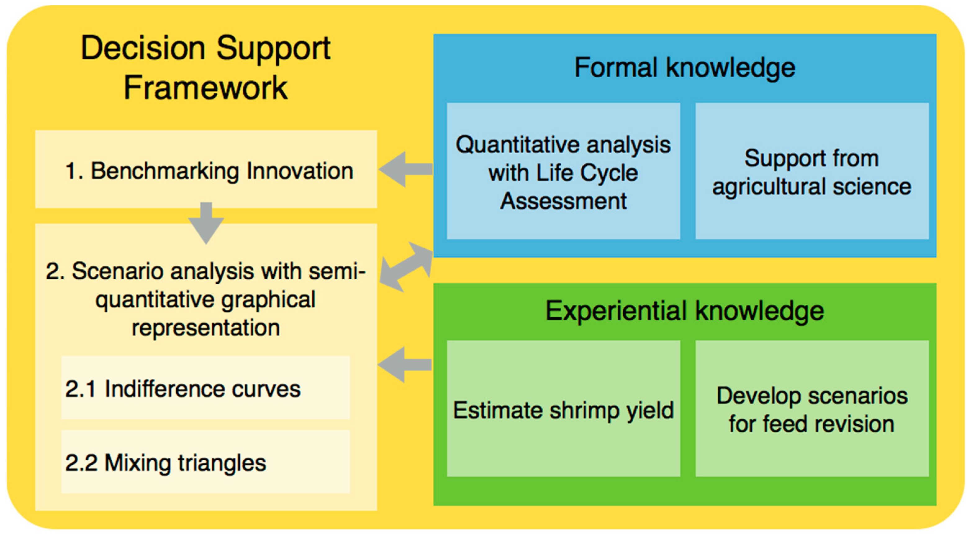
The decision support framework is developed through two main steps: benchmarking innovation (i.e., GWP performance and production cost of shrimp, introduced in Section 2.1), and scenario analysis with semi-quantitative graphical representation (i.e., indifference curves and mixing triangles, introduced in Section 2.2) [18]. Figure 2 illustrates the overall framework, showing the flow of formal and experiential knowledge. LCA, the core quantitative analysis method, is used to evaluate benchmark performance and scenarios. Farmer experiential knowledge is used to estimate shrimp yield and co-design scenarios for feed revision by supplementing agricultural science knowledge.

2.1. Benchmarking Innovation with LCA

The benchmark was set on a farm-scale experiment conducted by the farmer during January to September 2013. A common white shrimp species, Penaeus vannamei, was farmed with zero-exchange of water in a 2000-m² earthen pond for 245 days. This innovative ecological method was implemented with the application of heterotrophic bacteria to the pond at a 28-day interval, and feeding a total of 1953 kg of shrimp feed. The harvest was 815 kg of fresh shrimp.

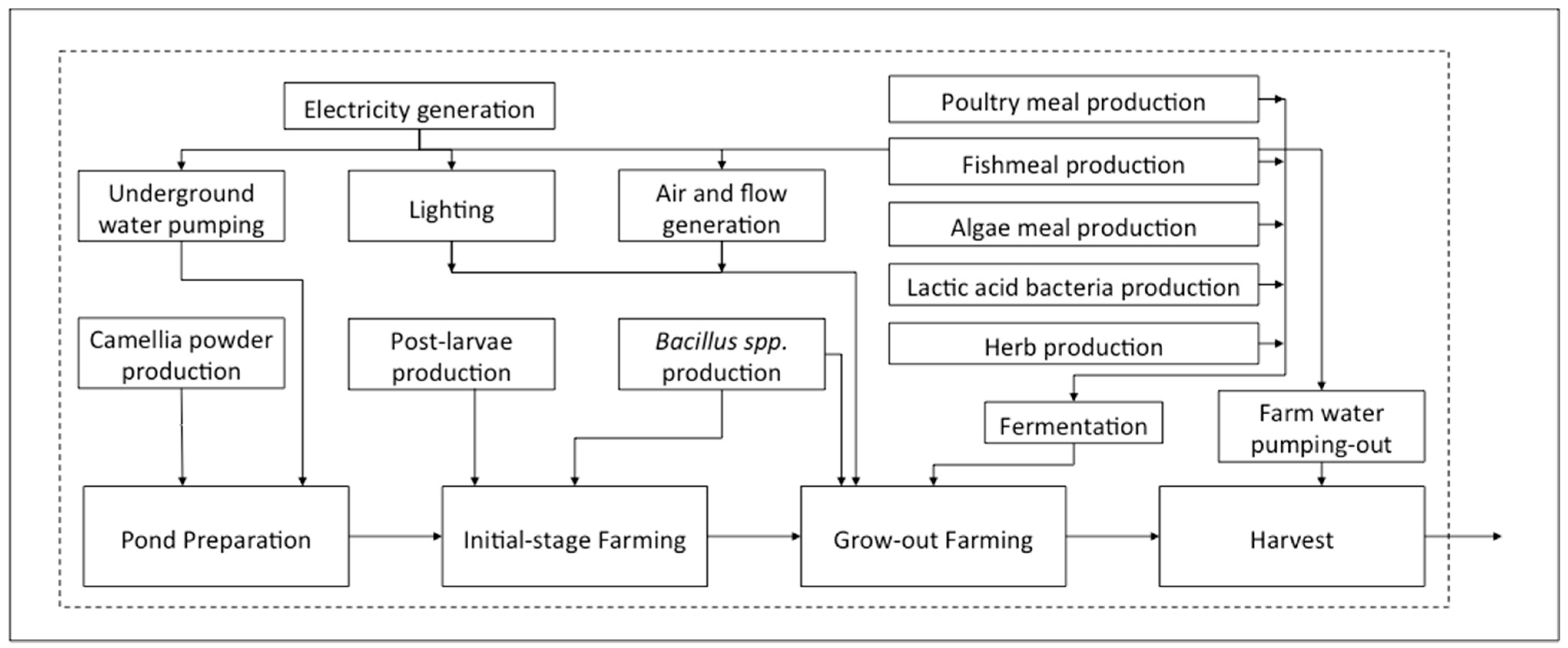
The environmental impact and economic performance of the innovation are quantitatively analyzed using the LCA methodology [20]. The life cycle scope is tailored from cradle to farm-gate (Figure 3). The four main farming stages are pond preparation, initial-stage farming, grow-out farming, and the harvest. Upstream processes include post-larvae production, camellia powder production, feed production, bacteria production, electricity generation, lighting, water pumping, and air and flow generation. After the harvest stage, the downstream processes are excluded because they are unrelated to the objective of improving shrimp farming.

Figure 2. The decision support framework shows two main operating steps—benchmarking innovation and scenario analysis, and the flow of formal and experiential knowledge. Life cycle assessment, the core quantitative analysis method, is used to evaluate the benchmark and scenarios. Farmer experiential knowledge is used to estimate shrimp yield and develop scenarios for feed revision by supplementing agricultural science knowledge.

Figure 2. The decision support framework shows two main operating steps—benchmarking innovation and scenario analysis, and the flow of formal and experiential knowledge. Life cycle assessment, the core quantitative analysis method, is used to evaluate the benchmark and scenarios. Farmer experiential knowledge is used to estimate shrimp yield and develop scenarios for feed revision by supplementing agricultural science knowledge.

Figure 3. The cradle-to-gate lifecycle stages in the ecological shrimp farming. Primary data are collected for pond preparation, initial-stage farming, grow-out farming, and harvest. A dotted rectangle indicates the cutoff of this study.

Figure 3. The cradle-to-gate lifecycle stages in the ecological shrimp farming. Primary data are collected for pond preparation, initial-stage farming, grow-out farming, and harvest. A dotted rectangle indicates the cutoff of this study.

We assumed there is no direct emission of methane from the farming stages, as measured data are not available. Shrimp farming with modified biofloc technology is expected to lower the carbon content, which is the source of methane formulation, due to its consumption by heterotrophic bacteria in the pond. In addition, the shrimp pond is aerated, so the contribution of methane emission is considered limited. Therefore, if our assumption does not apply, the consequence is likely to work in favor of current practice, rather than the new farming practice.

Primary inventory data in four main farming stages were collected through field survey and interviews with the farmer. Secondary data in upstream processes were adapted from the Ecoinvent Version 3 [21], a global LCA database, in the absence of raw data. Then, the environmental impact of GWP over 100 years was characterized in carbon dioxide equivalent units for GHGs according to the IPCC 2001 method [22]. The economic performance of production cost was calculated in Taiwanese Dollars (TWD); 1 TWD was approximately equivalent to 0.03 US dollar. The inventory result has been summarized in Table 1.

Table 1. Inventory result of material use quantity, cost, and global warming potential for the benchmark shrimp farming cycle that produced 815 kg of fresh shrimp.

Materials		Quantity a	Cost a (Taiwanese Dollar c)	Global Warming Potential （kg CO2 equiv.)	Reference for Global Warming Potential
Post-larvae	(number)	400,000	3998	211	[17]
Underground water b	(m3)	3000	-	-	-
Camellia powder	(kg)	200	2499	224	Ecoinvent v3
Fishmeal feed	(kg)	548	20,797	378	LCA Food DK
Poultry meal feed	(kg)	568	27,243	132	Ecoinvent v3
Algae meal feed	(kg)	831	52,358	108	Ecoinvent v3
Lactic acid bacteria	(kg)	4	2432	0.49	Ecoinvent v3
Herb supplement	(kg)	2	1216	0.31	Ecoinvent v3
Heterotrophic bacteria	(kg)	16	6397	1.94	Ecoinvent v3
Electricity	(kWh)	4108	14,762	2185	Taiwan EPA
Total			131,702	3240.74

^a The data is based on personal communication, collected in September 2013; ^b Cost and global warming potential are included in the inventory of electricity; ^c One Taiwanese Dollar is equivalent to approximately 0.03 US dollar.

Table 1. Inventory result of material use quantity, cost, and global warming potential for the benchmark shrimp farming cycle that produced 815 kg of fresh shrimp.

Materials		Quantity a	Cost a (Taiwanese Dollar c)	Global Warming Potential （kg CO2 equiv.)	Reference for Global Warming Potential
Post-larvae	(number)	400,000	3998	211	[17]
Underground water b	(m3)	3000	-	-	-
Camellia powder	(kg)	200	2499	224	Ecoinvent v3
Fishmeal feed	(kg)	548	20,797	378	LCA Food DK
Poultry meal feed	(kg)	568	27,243	132	Ecoinvent v3
Algae meal feed	(kg)	831	52,358	108	Ecoinvent v3
Lactic acid bacteria	(kg)	4	2432	0.49	Ecoinvent v3
Herb supplement	(kg)	2	1216	0.31	Ecoinvent v3
Heterotrophic bacteria	(kg)	16	6397	1.94	Ecoinvent v3
Electricity	(kWh)	4108	14,762	2185	Taiwan EPA
Total			131,702	3240.74

^a The data is based on personal communication, collected in September 2013; ^b Cost and global warming potential are included in the inventory of electricity; ^c One Taiwanese Dollar is equivalent to approximately 0.03 US dollar.

To make the LCA reusable for different inputs (from scenario analysis in Section 2.2), the computational model is built on Microsoft Excel using the matrix algebra structure, which formulates a collection of numbers arranged in a rectangular grid for systematic calculation [23]. Here, the system of product processes is encoded as vector p, wherein p contains input and output data of the unit process. The p is structured with two systems—A entries as economic flow (e.g., amount of materials and energy use), and B entries as environmental flow (e.g., GHGs emission per unit electricity generation) and cost. The structure of matrix-based LCA model can be represented in two Equations (1):

$$\begin{array}{l}As=f\\ Bs=g\end{array}$$

(1)

where s is the scaling vector, f is the desired final demand of the product system (or functional unit of product—1 kg harvested shrimp in this case), and g describes the total environmental interventions or cost for the product system. The equations can be summarized with the equation g = BA⁻¹f, allowing results of one complex system to be conveniently calculated even with different entries of input variable or A.

2.2. Scenario Analysis with Semi-Quantitative Graphical Representation

An interview-based discussion with the farmer was conducted to co-design the scenarios for improving the innovation. Two approaches were applied: changing the heterotrophic bacteria application frequency, and revising the feed input. For bacteria applied frequency, the farmer estimates that an applied interval within ± 8 days is possible without compromising the effect of improving pond ecology. For feed input revision, the alternatives of reducing total feed amount and changing poultry meal to wheat meal were proposed based on literature review (i.e., changing from protein-rich feed to carbohydrate-rich feed to promote heterotrophic bacteria growth based on the concept of biofloc technology [24]) and the minimum-feeding model. Prospective outcomes are divided into three possibilities: increase, decrease, or no change in shrimp yield.

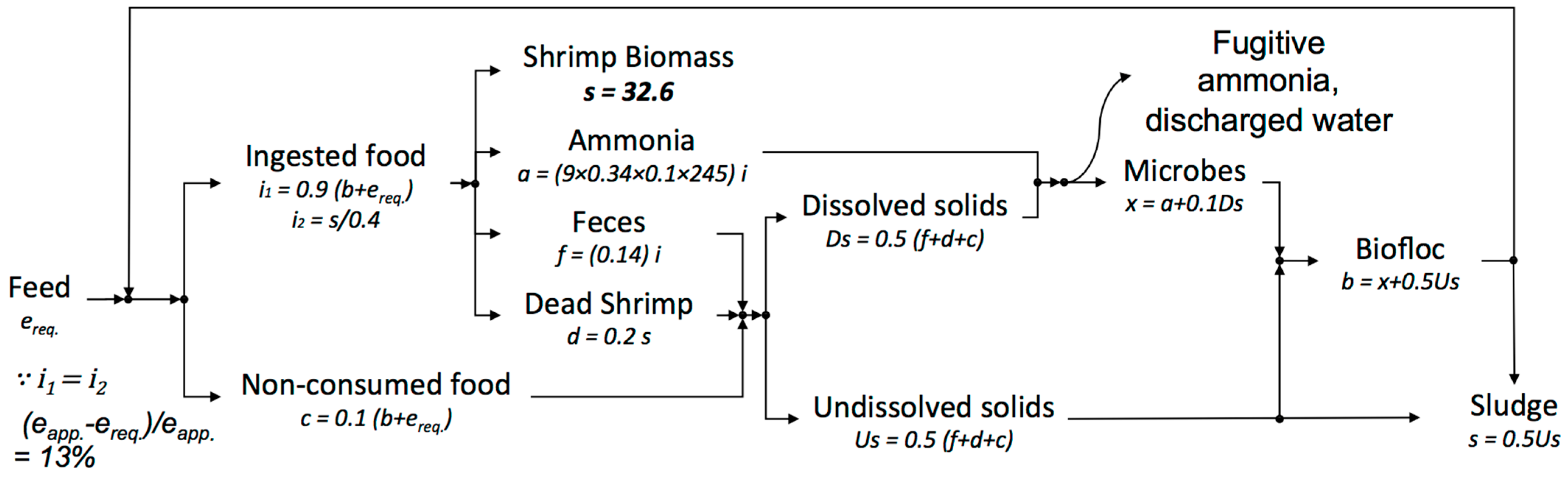
The minimum-feeding model is built on the mass balance of nitrogen in a pond system [25]. Nitrogen is assumed to be the proxy of available protein feed, a limited nutrient for shrimp growth. Therefore, modeling the nitrogen budget can serve as an estimation of the minimum required feed. The nitrogen pathway in the pond environment is synthesized in Figure 4. The relationships of each element are acquired or modified from aquaculture science studies [25,26]. Minimum required feed e_req. is estimated for a given shrimp biomass production, enabling the excessive feed amount in current feed input to be determined. The model shows a 13% feed reduction potential in the benchmark case.

Figure 4. Synthetic nitrogen pathway of pond environment based on aquaculture science shows 13% reduction potential for current applied feed (e_app.). The minimum feed required (e_req.) is determined through solving for ingested feed (i₂) and its associated units (i₁, b, c, e).

Figure 4. Synthetic nitrogen pathway of pond environment based on aquaculture science shows 13% reduction potential for current applied feed (e_app.). The minimum feed required (e_req.) is determined through solving for ingested feed (i₂) and its associated units (i₁, b, c, e).

From the above two approaches of alternatives and prospective outcomes, 22 scenarios are developed and summarized in Table 2, including 16 scenarios from the day interval of bacteria application, and six scenarios from two alternative feed input revision with three possible outcomes each. The bacteria application sets of scenarios are analyzed with the inclusion of farmer experiential knowledge in indifference curves, and the feed input sets of scenarios are in mixing triangle. These graphical representations provide only semi-quantitative results. The final interpretation shows if the alternative approach is better, worse, or the same relative to the benchmark.

Table 2. Scenarios for each approach, alternative, and prospective change of shrimp yield resulting from farmer discussion.

Approaches	Alternatives	Prospective Change of Shrimp Yield	Scenario Counts (No.)
Heterotrophic bacteria applied frequency	Applied within ± 8 days	Judged by farmer	16
Feed input revision	Reduce—13% reduction of total feed to minimum requirement	Increase by 10%, no change, decrease by 20%	6
	Replace—13% replacement of theoretical excess poultry meal to wheat meal	Increase by 10%, no change, decrease by 5%

Table 2. Scenarios for each approach, alternative, and prospective change of shrimp yield resulting from farmer discussion.

Approaches	Alternatives	Prospective Change of Shrimp Yield	Scenario Counts (No.)
Heterotrophic bacteria applied frequency	Applied within ± 8 days	Judged by farmer	16
Feed input revision	Reduce—13% reduction of total feed to minimum requirement	Increase by 10%, no change, decrease by 20%	6
	Replace—13% replacement of theoretical excess poultry meal to wheat meal	Increase by 10%, no change, decrease by 5%

2.2.1. Indifference Curves for Supporting Heterotrophic Bacteria Applied Frequency

The indifference curves methodology is adapted from economic theory [27]. It shows a curve where consumer preference of comparative products is indistinguishable, or the performances of comparative sets of variables are equivalent. Decision can be supported by judging whether the anticipated outcome falls on the advantageous or disadvantageous side of the curves.

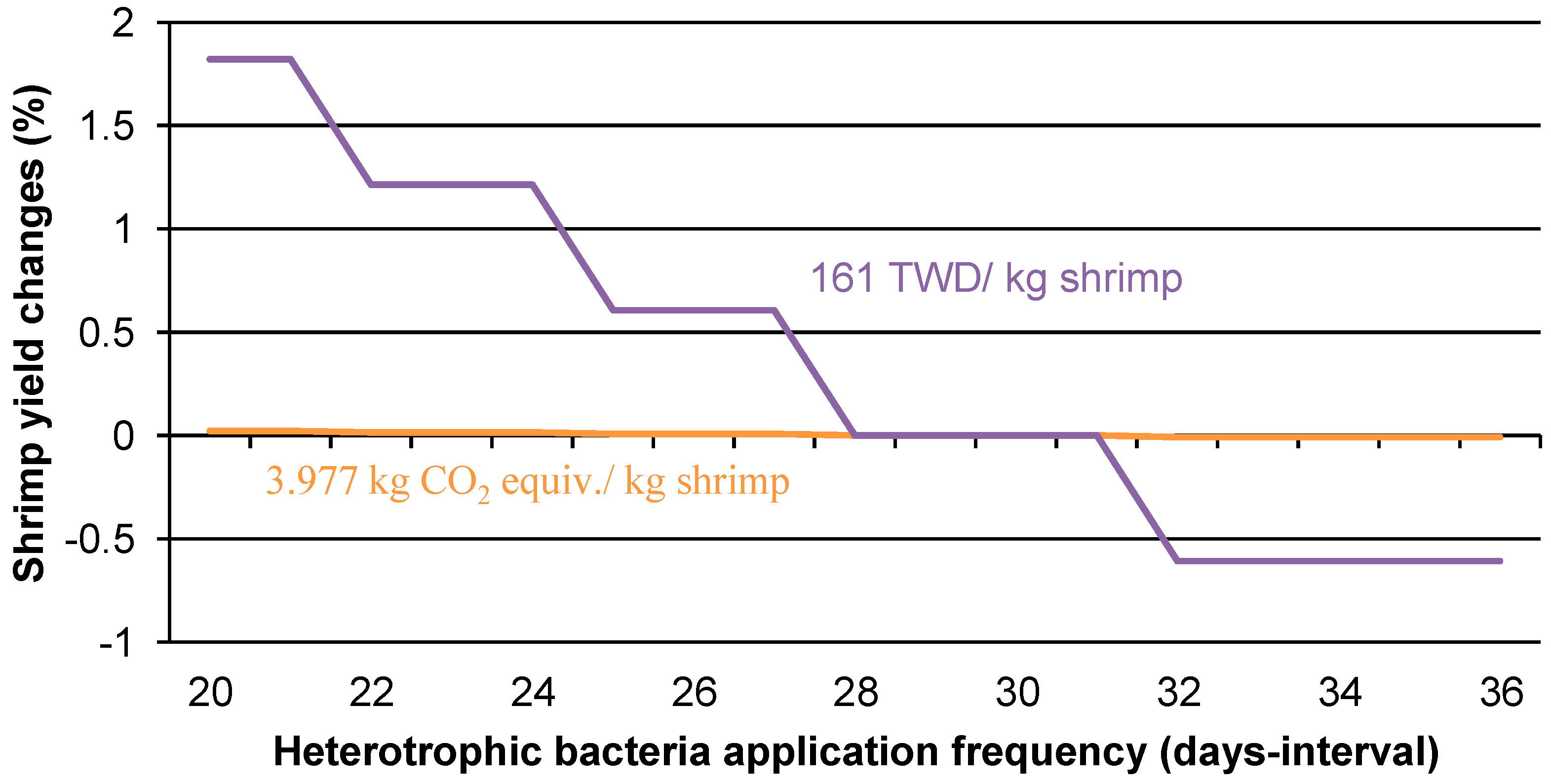
Here, the decision of heterotrophic bacteria applied frequency is supported. A line graph with two indifference-performance curves relative to the benchmark performance of GWP and cost of 28 days interval are drawn. To calculate the value of the curves, the LCA model developed in Section 2.1 is applied in a reverse manner—the GWP of shrimp production is assumed to be known and equivalent to the benchmark, and then the range of heterotrophic bacteria applied frequency is entered to calculate the required shrimp yield changes in the model. The same approach is applied to the cost of shrimp production. Two sets of resulting values, representing GWP and cost indifference curves, are then plotted on a two-dimensional line graph. The x-axis is the heterotrophic bacteria application frequency in days-interval unit, and the y-axis is the shrimp yield changes in percentage relative to the benchmark. The resulting graph is then presented to the farmer to judge the anticipated shrimp yield in response to changes in bacteria applied frequency.

2.2.2. Mixing Triangle for Supporting Feed Input Revision

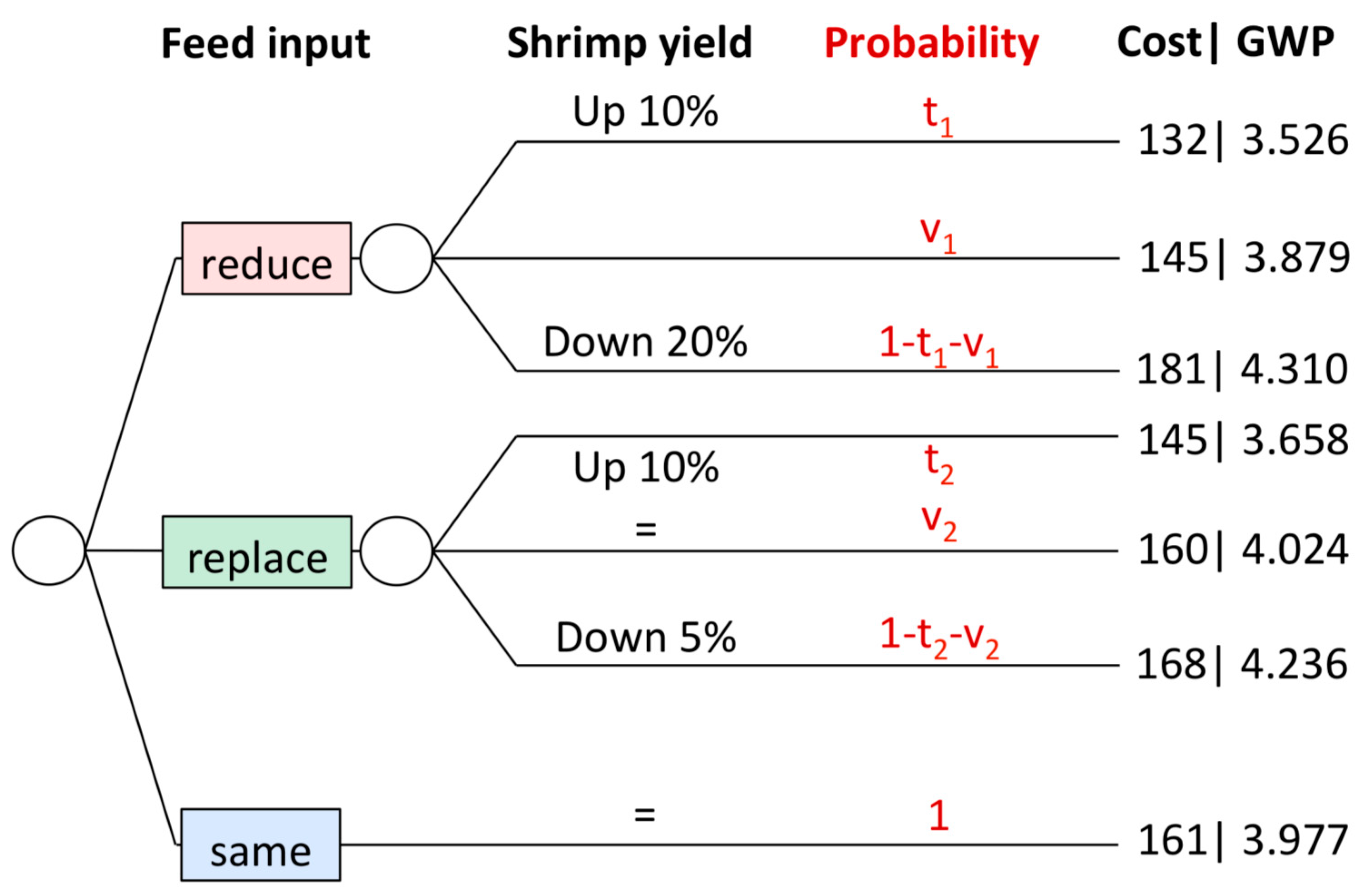
The mixing triangle method is developed based on the methodologies of Bayesian decision analysis [28,29] and the mixing triangle graphical representation [30,31]. Here, the mixing triangle is aimed at supporting the decision of feed input revision. A Bayesian decision tree treats the decision and uncertain events in procedural order; in a graphical sense, each decision is seen as a node and a node leads to alternate outcomes. The performance of each event (GWP and production cost) can be calculated in the LCA model. The expected value, which is the basis of comparison, is calculated by multiplying the conditional probability by the performance of each event. As illustrated in Figure 5, the scenarios for feed input are “reduce”, “replace”, and “same”. Feed input leads to the possibility of shrimp yields of “up 10%”, “=”, “down 20%”, and other combinations that are predicted by the farmer based on his experiential knowledge (details described in Table 2). The cost and GWP of 1 kg harvested shrimp for each set of feed input and shrimp yield is calculated using the LCA model developed in Section 2.1 (results in Figure 5). The probability of occurrence for each scenario is assigned as variables t and v. The expected value for each feed input is the summation of probability multiplied by the cost or GWP. Comparisons among the feed input options are made using linear inequality equations. Equations (2)–(4) are the inequality equations for comparing the cost expected value of “reduce” to “replace”, “reduce” to “same”, and “replace” to “same”, respectively. The same approach is applied to the GWP expected value.

$$132t+145v+181(1-t-v)<145t+160v+168(1-t-v)$$

(2)

$$132t+145v+181(1-t-v)<161$$

(3)

$$145t+160v+168(1-t-v)<161$$

(4)

Figure 5. Decision tree analysis showing the alternative feed inputs with possible shrimp yield changes. The probability of each scenario (variables t, v) is judged by the farmer. Cost and GWP are in TWD and kg CO₂-equiv. for each kilogram of shrimp production.

Figure 5. Decision tree analysis showing the alternative feed inputs with possible shrimp yield changes. The probability of each scenario (variables t, v) is judged by the farmer. Cost and GWP are in TWD and kg CO₂-equiv. for each kilogram of shrimp production.

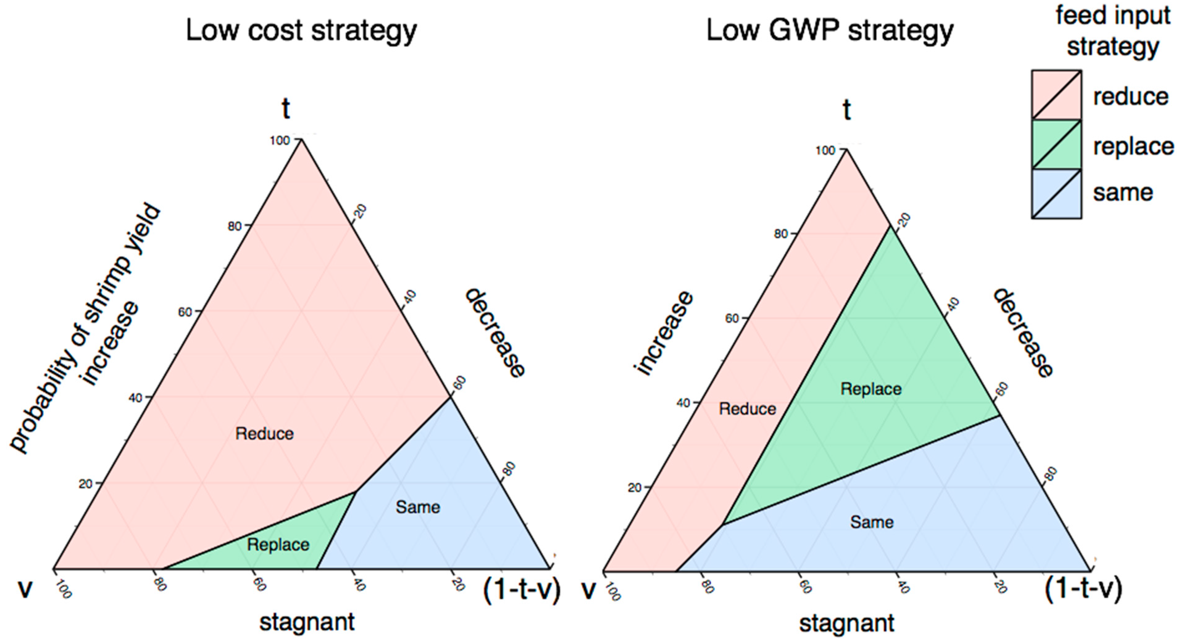
To best illustrate the comparisons of feed inputs, at three conditional probabilities, i.e., increase (t), decrease (1-t-v), and no change (v) to shrimp yields, the mixing triangle graphical decision support tool [30] is applied (illustration in Section 3.3). The conditional probabilities are represented on the three-side axes. The expected values of different feed inputs are compared and plotted in the triangle accordingly. The regions in the triangle are color-coded with the advantageous feed input revision, i.e., lower in GWP or cost. The mixing triangle graph is then presented to the farmer to judge the probability of each event based on experiential knowledge. Depending on the probability judgment of the farmer, advantageous strategies can be interpreted directly from the mixing triangles.

3. Results

3.1. Benchmarking Innovation with LCA

LCA results show the current performance of producing 1 kg of shrimp at farm gate as 161 TWD in cost and 3.977 kg CO₂-equivalent in GWP. Figure 6 shows the breakdown by process. Feed input, which includes algae meal, poultry meal, fishmeal, etc., costs up to 76%. The feed cost may vary from farm to farm depending on the feed mixtures. Heterotrophic bacteria are sensitive to cost, and applying 16 kg of bacteria contributes to 5% of total cost. Electricity generation contributes to 67% of GWP, mainly for powering the aerators, i.e., night-aeration is used to increase dissolved oxygen level for day and night. Feed production contributes 19% to GWP, which is much less than the electricity. Because the poultry meal and fishmeal are byproducts, the emissions are allocated by mass. For example, 1 kg fishmeal is produced for 0.208 kg fish oil; the emissions include the avoided rapeseed oil (which is replaced by the fish oil) in a consequential LCA.

Figure 6. Breakdown of life cycle processes of current shrimp production practice to global warming potential over 100 years (GWP) and production cost (cost) in percentage.

Figure 6. Breakdown of life cycle processes of current shrimp production practice to global warming potential over 100 years (GWP) and production cost (cost) in percentage.

3.2. Indifference Curves for Supporting Heterotrophic Bacteria Applied Frequency

The quantitative effect of applying heterotrophic bacteria to improve pond ecology and indirectly increase shrimp yield is unclear. A better practice means that the additional cost in applying bacteria more frequently can be compensated by the increasing in shrimp yield. Conversely, saving cost in applying bacteria less frequently does not necessarily result in a compromised shrimp yield. The decision of a farmer under such uncertainty is supported through indifference curves based on the compact information of lifecycle cost and GWP assessment.

Figure 7 shows the indifference curves of producing 1 kg shrimp in terms of GWP and cost based on a 28-day interval of bacteria application. These curves are the thresholds to determine the improvement of the bacteria application frequency. In practice, if we intend to increase the applied frequency to a 24-day interval, referring to the figure, the farmer must judge whether the prospective change in shrimp yield can achieve at least 1.2% to break even with the additional cost of purchasing the bacteria. If the anticipated change is better than the benchmark, then the improvement is recommended. If the anticipated change falls between GWP and cost curves, then a trade-off must be made. In this case, the GWP is very insensitive to heterotrophic bacteria application, thus increasing bacteria application for higher shrimp yield is always better for improving the GWP of farming 1 kg shrimp. Here, instead of relying on scientific proven theory, experiential knowledge is utilized as the basis of decision-making.

Figure 7. The indifference curves for supporting heterotrophic bacteria applied frequency. The purple curve shows the cost equivalence to benchmark of a 28-day interval (161 TWD/kg shrimp), and the orange curve shows the GWP (3.977 kg CO₂ equiv./kg shrimp).

Figure 7. The indifference curves for supporting heterotrophic bacteria applied frequency. The purple curve shows the cost equivalence to benchmark of a 28-day interval (161 TWD/kg shrimp), and the orange curve shows the GWP (3.977 kg CO₂ equiv./kg shrimp).

3.3. Mixing Triangle for Supporting Feed Input Revision

The current feed input amount is 13% more than the required amount based on our estimation (Figure 4). However, the theoretical minimum feed input is not definite due to the variation of ecology and biological growth. As a result of discussion with the farmer, we designed two alternative feed input revisions, “reduce” and “replace” (Table 2), where “reduce” represents a higher risk option comparing to “replace”. These strategies are then compared in a decision tree analysis (Figure 5) and plotted on mixing triangles to support a farmer in making a final decision on feed input.

Figure 8 shows the mixing triangles that were presented to the farmer. First, the conditional probabilities of shrimp yield changes (i.e., variables t and v on the axes) must be predicted based on the farmer’s experiential knowledge. Then, the farmer locates the point in the triangle and reads the color code to determine the most advantageous revision. For example, if the farmer feels that reducing the feed amount is unlikely to retard shrimp growth, he might therefore designate the probability of shrimp yield increase as 60%, that of decrease as 20%, and that of stagnation as 20%. Then, referring to Figure 8, the point drops to the red area (indicating a low-cost strategy), and green area (indicating a low-GWP strategy). This indicates that the strategy to “reduce” the feed has a higher chance of increasing profit but the strategy to “replace” is probably better for reducing GWP.

Figure 8. The mixing triangle shows decision support for feed input revision: low-cost strategy on left and low-GWP on right. The three-side axes show the probability of the prospective shrimp yield increasing, decreasing, or remaining stagnant relative to the benchmark. Color codes show the most advantageous strategy based on the expected value comparisons.

Figure 8. The mixing triangle shows decision support for feed input revision: low-cost strategy on left and low-GWP on right. The three-side axes show the probability of the prospective shrimp yield increasing, decreasing, or remaining stagnant relative to the benchmark. Color codes show the most advantageous strategy based on the expected value comparisons.

4. Discussion

The decision support framework is an attempt to solve the practical problems of farmers by utilizing their experiential knowledge to supplement LCA-based knowledge. The designed framework is understandable to the farmer, but the impact in implementation is limited. First, the sensitivity of some parameters can be too low to distinguish by experiential knowledge. In the indifference curve (Figure 7), the farmer must judge changes in shrimp yield on the y-axis. However, the thresholds to break even on both the benchmark GWP and cost are only 2% apart because the contribution of applied bacteria is small relative to feed and other inputs. Practically, involving the farmer to distinguish a better application frequency when only such minor change is involved is unfeasible. The indifference curve is therefore more applicable to the cases where changes are more significant. Second, in the mixing triangles (Figure 8), the three alternative strategies are evaluated based on one cycle of farming period, which takes about six to eight months, whereas the farmer normally predicts shrimp yield changes based on daily observation, and adjusts the feeding amount accordingly. The mixing triangles are therefore only useful for planning an overall feeding strategy. Third, the decision tools treat GWP and cost separately. Whenever a trade-off is encountered, the farmer must choose based on his normative experiential knowledge, which usually places a high priority on the profit of farming activity.

The framework is designed to complement LCA-based decision support with experiential knowledge. It is transferable to other case studies that have the following situations: (1) explicit scientific knowledge is insufficient, and (2) experiential knowledge is appropriate to make the necessary judgments. Beside the application in this shrimp farming study, the author has previously applied a similar concept to a case in Taiwanese sugarcane farming [18]. In the study [18], the indifference curves of GHG emission in the changes of N, P, and K fertilizer consumption, quantity of irrigation water, and times of inter-tillage were drawn based on LCA. The sugarcane farmers could decide the benefits of the above improvements by estimating the prospective change in corresponding sugarcane yield. To examine the effectiveness of transferring the proposed framework, more studies on different aspects of applications, notably in agricultural activity, should be explored.

This paper discusses only global warming among various impact categories in LCA. The decision support framework, however, is designed for a generic purpose. The assessment of GWP and other impacts are based on the formal knowledge of LCA (Figure 2); they can be performed individually using the same approach. We select GWP to assist the farmer in acquiring a carbon footprint label [32] for the shrimp product in this study. If more than one impact category must be addressed, the same graphical representations can be applied. The indifference curves (Figure 7), for example, must be updated with curves that reflect eutrophication, acidification, and other impacts. Similarly, the mixing triangles (Figure 8) can be layered to show the preference strategies for multiple impacts. However, as the impact categories increased, an increase in trade-offs between the impacts is likely to be encountered. Such trade-offs may complicate the decision-making process, making it less acceptable to the farmer. Another possible solution is aggregating the impact categories into a new indicator by scoring and weighting beforehand. Hofstetter et al. [30] show the aggregation of different environmental impacts, i.e., pesticides, greenhouse effects, acidification, and eutrophication, based on a universal scoring method in the Eco-indicator 95 in a study of mixing triangles application. This aggregated indicator can be easily adapted to our decision support framework. To summarize, the potential of the decision support framework goes beyond mere assessment of global warming; however, there is a need of further study on how to choose from various methodological options in incorporating all of the relevant impact categories into practical decision-making.

5. Conclusions

A decision support framework is developed to systematically utilize experiential knowledge in an LCA-based framework, notably in the scenario analysis with two semi-quantitative graphical representations of indifference curves and mixing triangles. The presented shrimp farming case demonstrates the use of our proposed framework. We assigned the uncertainty judgment to the farmer while taking the responsibility for removing the complexity of cost and environmental performance across the product’s life cycle. This approach is particularly useful in agricultural studies because acquiring a sufficient volume of data from experiments may be too costly in terms of time and money. Farmer experiential knowledge is assumed to be a reliable alternative source to supplement scientific knowledge.