Impacts on CO₂ Emission Allowance Prices in China: A Quantile Regression Analysis of the Shanghai Emission Trading Scheme

Abstract

A pilot regional carbon emission trading scheme (ETS) has been implemented in China for more than two years. An investigation into the impacts of different factors on carbon dioxide (CO₂) emission allowance prices provides guidance for price-making in 2017 when the nation-wide ETS of China will be established. This paper adopts a quantile regression approach to estimate the impacts of different factors in Shanghai emission trading scheme (SH-ETS), namely, economic growth, energy prices and temperature. The empirical analysis shows that: (i) the economic growth in Shanghai leads to a drop in the carbon allowance prices; (ii) the oil price has a slightly positive effect on the allowance prices regardless of the ordinary least squares (OLS) or quantile regression method; (iii) a long-run negative relationship exists between the coal price and the Shanghai emission allowances (SHEA) prices, but a positive interaction under different quantiles, especially the 25%–50% quantiles; (iv) temperature has a significantly positive effect at the 20%–30% quantiles and a conspicuous negative impact at the right tail of the allowances prices.

1. Introduction

The global warming arising from continuous economic progress is a persistent and serious challenge to the world. As a major greenhouse gas (GHG) emitter, China has worked hard to cut GHG emissions, and incorporated a series of explicit goals into the Chinese Five-Year Plan [1]. For instance, the latest target of controlling climate change was identified in 2015, when the Chinese government made a commitment to reduce 60%–65% of carbon intensity by 2030 relative to the level in 2005 and reach its peak of carbon emission in 2013 or earlier [2]. China has taken various measures to achieve the targets of emission reduction, and it has been revealed that the most efficient solution is to proceed with carbon emission trading [3].

The Chicago Climate Exchange (CCX) and the European Union Emission Trading Scheme (EU-ETS) are, respectively, representative of voluntary and mandatory emission reductions [4]. The CCX began carbon emissions trading in 2003. The EU-ETS, set up in 2005, is currently the world’s largest carbon emissions trading market [5]. Seven pilot provinces and municipalities in China, namely, Guangdong, Shenzhen, Beijing, Shanghai, Hubei, Tianjin and Chongqing, have gradually lunched their emission trading schemes in 2013. A growing attention is focused on the issues with the carbon trading markets that have operated actively for over two years, e.g., total amount of control, allowances allocation, allowances releases, trading, verification and allowances offset. Meanwhile, China is accelerating the construction of a nation-wide ETS, which is expected to be completed in 2017. On China’s carbon emission website [6], the market prices of emission allowance in seven pilot regions differ significantly. Reasonable allowance prices can improve the effectiveness of carbon emission markets in cutting emissions. Therefore, relevant empirical studies of the carbon pricing schemes in the indispensable ETS in China must be necessary to work out some useful strategies for domestic ETS. In this paper, we aim to use Shanghai emission trading scheme (SH-ETS) as an example to estimate the impacts upon CO₂ emission allowance prices.

SH-ETS was launched on 26 November 2013 and included 191 firms. It was based on the carbon emissions during 2010–2011. Emitters can receive allowances from initial allocation based on previous carbon emissions every year, meanwhile they are obliged to accept a verification and settle emissions allowances based on actual carbon emissions in the middle of the year. Hence, emitters with excessive carbon emissions need to buy Shanghai emission allowances (SHEA) or China certified emission reductions (CCER) for offsetting with some limitations on the ratio of CCERs offset. We use SH-ETS as a case study due to its market mechanism and trading status. (i) According to the Shanghai Statistical Yearbook [7], Shanghai reached 2.36 trillion yuan in gross domestic product (GDP) and total energy consumption of the equivalent of 110.85 million tons of coal in 2014. It is compulsory for the Chinese central government to make a 19% cut in the carbon intensity during the 12th five-year plan, based on development stage and resources endowment; (ii) SH-ETS operated with the most detailed and sophisticated market rules among seven pilot regions. The total volume of Shanghai emission allowances (SHEA) and CCERs, which ranked first among the seven pilot provinces and municipalities, attained 30.37 million tons with a total value of more than 467.48 million yuan until the end of 2015; (iii) SHEA price features high volatility. As shown in Figure 1 [6], it started at 26.42 yuan/ton and soared sharply to 46 yuan/ton in February 2014. The price remained at around 40 yuan/ton until the end of June 2014, but experienced a reform for two months and no trading. Then it fluctuated in a range of 25–35 yuan/ton over half a year and continuously dropped to around 10 yuan/ton in 2015. Hence, it is representative of the impacts on allowance prices for SH-ETS.

There has been considerable research regarding impact factors for carbon emission allowance prices since the emergence of CCX and EU-ETS. Numerous studies have identified that energy prices are the price determinants of allowances [8,9,10,11,12]. For example, Bunn and Fezzi [8] applied a cointegrated vector error correction model to highlight the interactions and dynamic pass-through among electricity, gas and carbon prices. Kim and Koo [9] and Lahiani et al. [11] utilized linear and nonlinear autoregressive distributed lags model to estimate the impacts of energy prices on CO₂ emission allowance prices, respectively. The former found that the main determinant of allowance trading was coal price in the long-run, but the latter found asymmetric and nonlinear relationships among variables. Hammoudeh et al. [12] emphasized the short-term dynamics by a Bayesian Structural vectorial autoregression (VAR) approach. In light of the abatement options on large installations, Keppler and Mansanet-Bataller [13] reported that coal and gas prices, through clean dark spreads (CDS) and clean spark spreads (CSS), had an influence on carbon prices, which in turn Granger caused electricity prices for Phase I of the EU-ETS. Bredin and Muckley [14] investigated additional fundamentals such as equity prices, temperature deviations, and CDS and CSS by using the Johansen cointegration test. Wang and Bai [15] found that CDS and CSS had a positive and negative effect on allowance prices in EU-ETS, respectively and other studies took account of the switching behavior between gas and coal [16,17]. Relying on the cointegration method, Creti et al. [17] investigated the relationships between carbon price and its drivers (oil price, the switching price between gas and coal, equity price index) during Phases I–II of the EU-ETS and showed that the equilibrium relationships existed in both phases, especially in Phase II. The switching price did not work in Phase I. Additionally, weather conditions have been incorporated into studies and shown important influence on the allowance prices [18,19,20,21,22]. Rickels et al. [18] acknowledged that the allowance prices react to changes in energy prices and weather when the allowances are regarded as a scarce input factor. Mansanet-Bataller et al. [19] aimed to consider the underlying rationality of pricing behavior and found that that energy resources are the principal factors to determine the carbon price levels, which were also affected by extreme temperatures. Chen et al. [21,22] separately assessed the impacts of changes in energy prices and climate factors (precipitation, weed and temperature) on allowance prices in EU-ETS and CCX, and pointed out that only temperature had a significant negative effect among climate factors in CCX. The equal importance of industrial production and macro-economy in relation to carbon price has been shown by many researchers [23,24,25,26]. Christiansen et al. [23] showed the role of two proxies (industrial production and equity price movements) on the price of emission allowances in the EU-ETS in 2005–2007. Chevallier [25] used the Markvo-switching model to assess the impacts of economic activity (aggregated industrial production) and energy prices (Brent, natural gas and coal prices) on European Union Allowances. Conraria and Sousa [26] found that a shock in economy index prices had an effect on carbon prices, but there was no significant impact of the substitution for carbon licenses in Phases II–III of the European market.

A strand of previous literature has focused on the issues and mostly described the average impact among variables, failing to process the effects of extreme distribution, and leading to the loss of partial information. Only Hammoudeh et al. [27] analyzed the impact of four energy prices on the European Union CO₂ emission allowance prices by the quantile regression. Quantile regression has been widely employed in empirical studies [28,29,30,31,32,33,34,35,36,37,38]. Many scholars used the quantile regression approach to investigate the dynamics of changes in different wage distribution [28,29,30] and dynamic relationship between exchange rate and stock price [31,32,33]. Recently, a growing number of studies have applied quantile regression to explore issues of carbon emissions [37,38]. For instance, Zhang et al. [37] utilized a quantile regression method to analyze the relationship between corruption and carbon emissions in Asia-Pacific Economic Cooperation (APEC) countries. Xu and Lin [38] estimated the impacts on China’s provincial carbon emissions by using quantile regression.

This paper has adopted the quantile regression method to assess the interactions between the price of the CO₂ emission allowances and different impact factors (macroeconomic, energy and climate factors). The contributions of this paper lie in three main areas. First, compared with available literature, there is little information about the impact factors on allowance prices in China’s carbon emission market. Second, we utilize the quantile regression to estimate whether the drivers consistently influence the CO₂ emission allowance prices through the conditional distribution in SH-ETS, providing a more complete picture. In particular, we reinforce the study by Hammoudeh et al. [27] and take into account other probable driving forces besides energy factors by summarizing previous literature.

The reminder of this paper is structured as follows. Section 2 presents the data collection and introduces the quantile regression model. Section 3 describes and discusses the interactions among the macroeconomic, energy, climate factors and SHEA prices through the quantile regression, and compares the results with the ordinary least squares (OLS) approach. Section 4 concludes the results with several policy implications.

2. Materials and Methods

2.1. Data

This paper estimates the impact factors on CO₂ emission allowance prices in SH-ETS and makes an analysis of daily time-series covering the dates from 26 November 2013 to the end of 2015. There are one dependent variable and four explanatory variables in our empirical analysis, namely SHEA price, Shanghai Composite Index (SZZS), fuel oil price, steam coal price and temperature, respectively. All variables were summarized in

Table 1. All dependent and explanatory variables.

Variable		Unit
Dependent variable	SHEA	Yuan
Explanatory variable	SZZS	Percent
	Fuel oil	yuan/ton
	Steam coal	yuan/ton
	Temperature	degree Centigrade

.

The data on SHEA are derived from the official website of China’s carbon emissions trading. The daily SZZS, collected from the China Stock Market and Accounting Research (CSMAR) Solution, represents the economic level of Shanghai. The energy variables are processed by future prices of fuel oil and steam coal, which are obtained from the Shanghai Futures Exchange (SHFE) and Zhengzhou Commodity Exchange (ZCE) separately. The selection of energy variables has taken two aspects into consideration. In China, the makeup of total energy consumption attributed to oil, coal, gas and electricity are respectively 17.1%, 66%, 5.7%, 10.2% in 2014, according to the China Statistical Yearbook [39]. In addition, future energy prices are the reference of spot prices by Keppler and Mansanet-Bataller [13]. Bredin and Muckley [14], Creti et al. [17], and Xiaohong Chen et al. [21,22] have also selected future energy prices as energy variables rather than spot prices. The daily data of the temperature in Shanghai are from the China Weather website [40], which reports weather conditions of China’s cities. Finally, we extract the overlapping data of five variables and delete the data when the trading volume is null, in consideration of the availability and efficiency of the data set. Finally, 341 observations are covered in the sample data.

Table 2. Descriptive statistics of dependent and explanatory variables.

Variable	Obs.	Mean	Max	Min	Std. Dev.	Skewness	Kurtosis
SHEA	341	30.35	48.00	9.50	8.38	−0.86	0.11
SZZS	341	2936.52	5166.35	1991.25	907.99	0.68	−0.71
Fuel oil	341	3480.07	4809.29	2007.00	604.31	−0.06	−0.59
Steam coal	341	477.56	595.60	290.04	68.46	−0.83	0.48
Temperature	341	14.78	34.00	1.50	7.84	0.22	−1.08

represents the descriptive statistics of dependent and explaining variables. We can observe that all variables deviate from normal distributions and are skewed in terms of skewness level. All values of the kurtosis are below three, indicating thinner tails rather than normal distributions. Quantile regression has no assumption about the normal distribution of variables [38]. Additionally, the high volatility of SHEA prices, ranging from 9.5 yuan to 48 yuan, makes the conditional distribution of prices feasible [35].

2.2. Methodology

To investigate the interactions between the price of the CO₂ emission allowances and different impact factors (macroeconomic, energy and climate factors), we account for the impacts on allowances prices by a quantile regression approach, which was first proposed by Koenker and Bassett [41]. The advantages of quantile regression are mainly three-fold. Firstly, the quantile regression approach is insusceptible to influences of outlier observations, skewness, and heterogeneity on explaining variables [42]. It achieves better robustness of the outliers. Secondly, quantile regression requires no error terms distribution and can make a more efficient estimation. Finally, it obtains nonlinear relationships and estimates the impacts for several quantiles of the distribution for the dependent variable [35]. Hence, it describes the full picture of conditional distribution on a dependent variable, especially the tail location, vis-a-vis the OLS method.

Given a random variable Y with a distribution function F(y) = Prob (Y ≤ y), the $\tau$ quantile of Y is defined as minimizing the y of F(y) ≥ $\tau$, and the inverse function is specified as follows:

$$Q\left(\tau \right)=\inf \left\{y:F\left(y\right)\ge \tau \right\},0<\tau <1$$

(1)

The parameters are estimated by minimizing the sum of absolute residuals as follows:

$$Q\left(\tau \right)=argmi{n}_{\delta }\left\{{\displaystyle \sum }_{i=1}^n{\rho }_{\tau }\left(y_i-\delta \right)\right\}$$

(2)

and Equation (2) can be transformed to the following:

$$argmi{n}_{\delta }\left\{{\displaystyle \sum }_{y_i\ge x_i^T\beta }\tau \left|y_i-x_i^T\right|+{\displaystyle \sum }_{y_i>x_i^T}\left(1-\tau \right)\left|y_i-x_i^T\right|\right\}$$

(3)

where $\tau$ ranges from 0 to 1, $\beta$ is the coefficient vector across the quantile of $\tau$ and varies with a specific $\tau$. The quantile regression can capture the impacts of explanatory variables on the distribution of dependent variable whatever value $\tau$ is.

The loss function of the quantile regression model is shown below:

$${\rho }_{\tau }\left(\mu \right)=\mu (\tau -I(\mu <0))$$

(4)

where I is an indicator function.

To estimate the impacts of changes in SZZS, energy prices (fuel oil and steam coal) and temperature on ${\mathrm{CO}}_2$ emission allowances prices in different quantiles, we establish a quantile regression model according to Hammoudeh et al. [27], which is displayed in Equation (5):

$$Q_{y_t}(\tau |x_t)=\alpha \left(\tau \right)+\gamma \left(\tau \right)SZZ{S}_t+\sigma \left(\tau \right)oi{l}_t+\phi \left(\tau \right)coa{l}_t+\omega \left(\tau \right)tem{p}_t+\epsilon \left(\tau \right),0<\tau <1$$

(5)

where $y_t$ is the dependent variable (SHEA price), $SZZ{S}_t$ donates the Shanghai Composite Index, $oi{l}_t$ and $coa{l}_t$ are the prices of fuel oil and steam coal, and $tem{p}_t$ is the daily temperature of Shanghai. $\gamma \left(\tau \right)$, $\sigma \left(\tau \right)$, $\phi \left(\tau \right)$ and $\omega \left(\tau \right)$ are the slope coefficients estimating the nonlinearity relationship between $y_t$ and four explanatory variables under $\tau$ quantile. $\epsilon \left(\tau \right)$ is the error term. After daily time series analysis, we find that daily time series are unstable and have no co-integration equation. Hence, we take logarithm of data in consideration of instability, and the five variables are presented as lnSHEA, lnSZZS, lnoil, lncoal and lntemp respectively after the logarithm [35].

The final adjusted formula is:

$$Q_{y_t}(\tau |x_t)=\alpha \left(\tau \right)+\gamma \left(\tau \right)lnSZZ{S}_t+\sigma \left(\tau \right)lnoi{l}_t+\phi \left(\tau \right)lncoa{l}_t+\omega \left(\tau \right)lntem{p}_t+\epsilon \left(\tau \right), 0<\tau <1$$

(6)

3. Results and Discussion

Before the regression estimation, it is necessary to apply the Augmented Dickey and Fuller (ADF) [43] unit root tests to evaluate the stability of time series. Stationary sequence can avoid the existence of spurious regression [38]. We have taken the logarithm of all variables and conducted the unit root tests for new sequences. The results of the tests for the unit root in level suggest that most variables are non-stationary, except for lncoal. Moreover, tests for the unit root at the first-order difference all refuse the null hypothesis at the 1% significance level, which shows that all variables in the first-order difference are stable. All evidence is shown in

Table 3. The Augmented Dickey-Fuller (ADF) unit root tests.

Variable	ADF Value	1st Difference of ADF
lnSHEA	−1.064833	−22.58128 ***
lnSZZS	1.211579	−14.48983 ***
lnoil	−1.217713	−17.76263 ***
lncoal	−2.305738 **	−27.39583 ***
lntemp	−0.603371	−13.30092 ***

Notes: There is no trend or intercept included in the test equation. The asterisks ***, **, * denote a significance level of 1%, 5%, 10%, separately.

. Under such circumstances, we establish the (VAR) model and use the Johansen test to verify a long-term co-integration relationship among several logarithm series, which was introduced by Jahansen [37,38,44] (The Johansen test is based on the establishment of the VAR model. It is appropriate for un-stationary time series, and is often implied for judging the long-run co-integration relationship among all variables. We need to use the Johansen test to overcome spurious regression for variables, which are stationary under first-order difference.) The result in

Table 4. Unrestricted cointegration rank test (trace).

Hypothesized No. of CE(s)	Eigenvalue	Trace Statistic	0.05 Critical Value	Prob.**
None *	0.124383	70.73127	69.81889	0.0422
At most 1	0.037331	25.83582	47.85613	0.0945

Notes: The asterisk * denotes rejection of the hypothesis at the 0.05 level. The asterisk ** donates Mackinnon-Haug-Michelis (1999) p-values.

indicates that there exists one cointegrating relationship at the 0.05 level.

Compared with the OLS regression model, employing a quantile regression method can attain more complex and detailed estimation results of an explanatory variable on dependent variables under the distribution of the SHEA prices. The different estimation results are shown in

Table 5. Results of ordinary least squares (OLS) and quantile regression estimations.

Variable	Ols	10%	25%	50%	75%	90%
α	9.21008 ***	−5.825944	−6.110953 ***	−6.664879 **	0.034741	5.215025
lnSZZS	−0.221336	−0.248885	−0.222590 ***	−0.141646	−0.256483	−0.442152 ***
lnoil	0.112685	0.639462	0.205251	0.244556 *	0.173301	0.127672
lncoal	−0.830799 ***	0.893984 *	1.481077 ***	1.501282 ***	0.679181	0.148548
lntemp	−0.074253 ***	0.047651	0.143950 ***	−0.008275	−0.029189	−0.043573 ***
AR(1)	0.990766 ***	-	-	-	-	-
D.W	2.309793	-	-	-	-	-

Notes: The asterisks ***, **, * still denote a significance level of 1%, 5%, 10%, separately. In the quantile regression analysis, the confidence interval is 95% and the τ quantiles we select include the tails and the median of distribution, such as 10%, 25%, 50%, 75%, 90%.

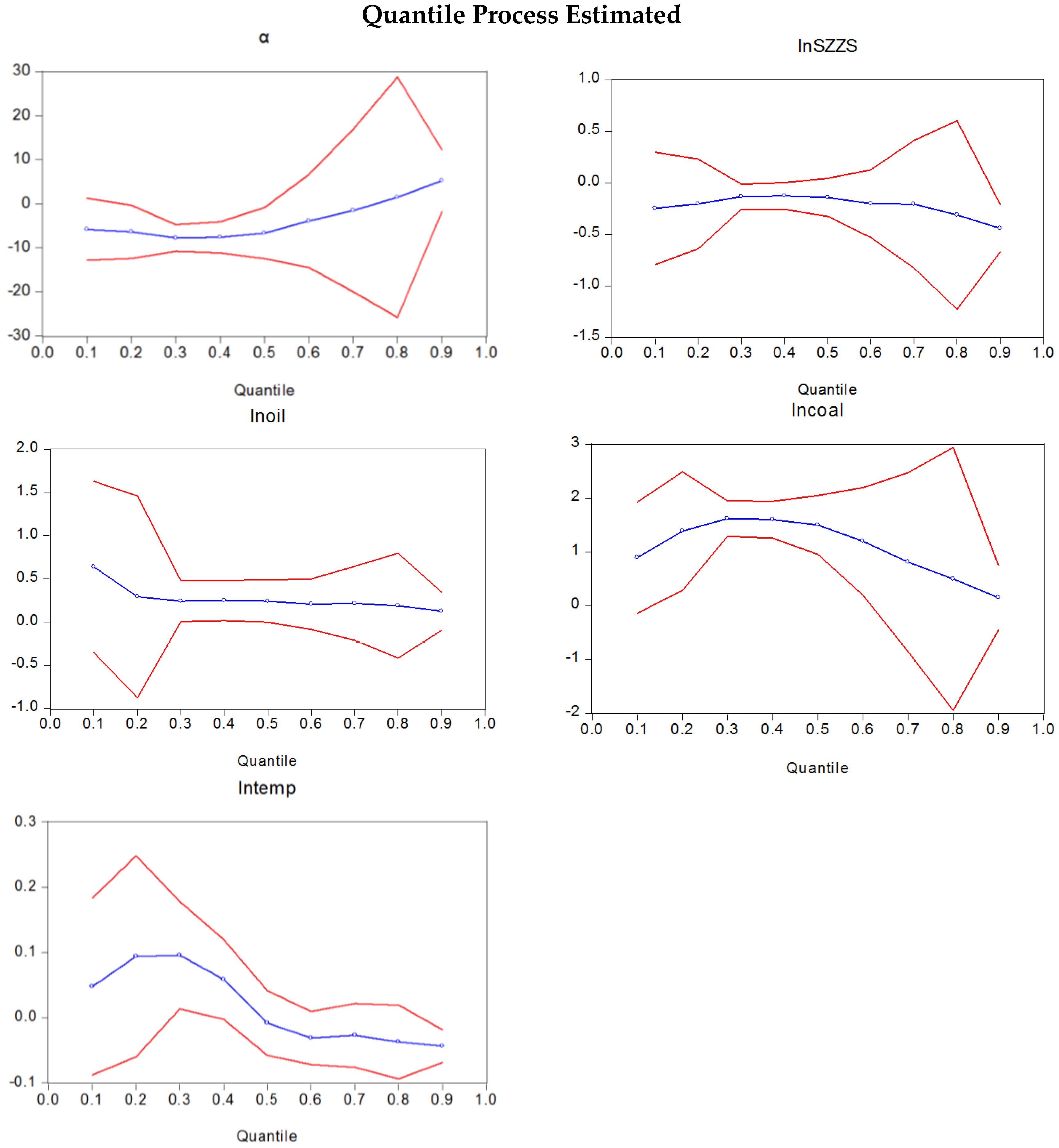
. We observe the Durbin-Watson [45] stat and find the existence of the sequence auto-correlation in the OLS regression estimation. Thus, we adopt the Cochrane-Orcutt [46] iterative procedure to make modification [47,48], and the Durbin-Watson stat rises to 2.309793 from 0.248561, which indicates that there is no longer auto-correlation on the verge of 2 [49]. Additionally, we can estimate the extent of impacts between variables by the slope coefficient under τ quantiles (τ = 10%, 25%, 50%, 75%, 90%) in Figure 2.

As for the effect of the SZZS on CO₂ emissions allowance prices in SH-ETS, the result indicates that there is a significantly negative effect at the 25% and 90% quantiles. Also, as is shown in Figure 2, the slope coefficients of SZZS fluctuate slightly. This means that the economic growth leads to a drop in allowance prices in Shanghai. This is unexpected and inconsistent with Wang and Bai [15]. However, Creti et al. [17] showed a negative relationship between economic growth and carbon prices in Phase I of the EU-ETS, which suggested that CO₂ allowances increased the diversification of a financial portfolio in a context of low environmental constraint [4]. Bredin and Muckley [14] found that equity price has a negative impact in Phase II of the EU-ETS and is likely due to the dramatic events on stock markets. The finding in this paper may be attributed to relatively low CO₂ intensities in Shanghai [50,51]. Hence, it achieves the CO₂ emissions mitigation with economic growth, leading to higher allowances prices.

Regarding the effect of fuel oil price on SHEA prices, the results of OLS and quantile regression all show that the effect is positive but not significant, and the slope coefficients have a slight, continuous decrease, which means the impact is stronger at the lower quantiles. Previous literatures about the effect of oil price on allowance prices are contradictory. This positive effect is consistent with Creti et al. [17], but inconsistent with the study by Lahiani et al. [11] and Hammoudeh et al. [27]. Hammoudeh et al. [27] found that oil prices had a stronger negative relationship with carbon prices at the right tail of the distribution. An increase in oil price generally generates a passive effect on allowance prices owing to falling energy demand. This impact of oil price on SHEA price may be caused by a strong demand for oil, especially at the beginning of SH-ETS operation.

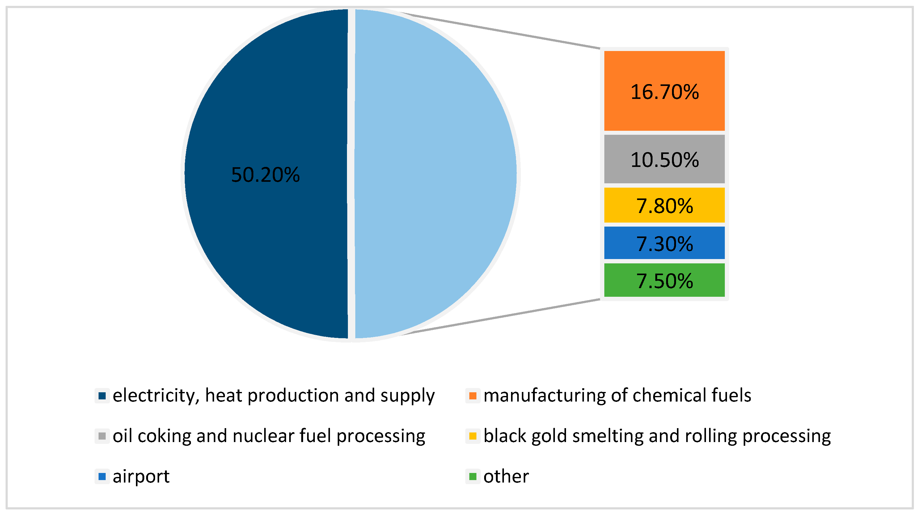
Regarding the impact of steam coal prices on SHEA prices, the OLS regression result suggests that there is a negative long-run relationship, which differs from the quantile regression estimation. An increase in steam coal prices generates a decline in coal demand, leading to the allowance prices generally falling. This long-run negative relationship has been demonstrated by Kim and Koo [9]. However, the effect of higher steam coal price on the prices of the allowance prices is significant and positive at the 25%–50% quantiles in Shanghai. One possible explanation for this finding is that natural gas can be substituted for coal in power generation when the latter’s price is higher. Electricity, heat production and supply sectors are the major traders in SH-ETS, according to Shanghai’s carbon market report [52]. The trading volumes ratios of SHEAs and CCERs have reached 50.2% in all sectors, as shown in Figure 3. More natural gas instead of coal in electricity, heat production and supply sectors continuously increases the carbon emissions and leads to increasing allowance prices. This positive effect may also be attributed to a strong coal demand, particularly when the allowance prices are low.

Finally, we can establish the superiority of the quantile regression in relation to the OLS regression model when we estimate the impact of the temperature on the allowance prices. The temperature has a significantly positive effect at the 20%–30% quantiles and an obvious negative influence at the right tail of the allowance prices distribution. Chen et al. [21,22] found that temperature only had a subtle positive influence in Phase II of the EU-ETS, but there is a significant negative impact on carbon prices in CCX. A positive relationship at the left quantiles due to the rising temperature is attributed to the increasing use of air conditioners in Shanghai where the medial temperature is on the high side compared to the rest of the country. On the other hand, a negative impact can be explained in a particular condition of domestic carbon emissions trading status. In SH-ETS, emitting firms which fail to meet emission reductions can buy allowances from those which make extra emissions cuts or they can buy CCERs from approved Clean Development Mechanism (CDM) projects for offsetting before June, leading to less demand later. The temperature of Shanghai reaches a peak in July and August, leading to a falling price of SHEAs, even though the temperatures rise.

4. Conclusions and Policy Implications

This paper tries to estimate impact factors (economy, energy and weather) on the CO₂ emission allowance prices through a quantile regression model, with a case study of SH-ETS because of the deficiency in research on China’s carbon emission markets at present. The empirical results for the SH-ETS demonstrate that economic growth has a significantly negative effect at the 25% and 90% quantiles, which means that economic growth in Shanghai generates a drop in carbon allowance prices. This may be due to relatively low CO₂ intensities in Shanghai and imply that Shanghai has taken some measures to decrease carbon emissions. This finding suggests that China should maximize the potential of the domestic carbon emissions trading market and encourage firms to develop more CDM projects. Trading of CCERs is a significant measure for emission allowance price adjustment, especially when the latter can only increase by a limited amount.

As for the energy prices, we find that the oil price has a slight and positive interaction with the allowance prices regardless of the OLS or quantile regression in SH-ETS. In general, the coal price has a negative relationship with the allowance prices because a higher coal price reduces the coal demand and subsequently drives the allowance price down. However, there is a positive effect under all quantiles, especially the 25%–50% quantiles. The positive effects may be due to the substitution of coal by gas in power generation, or a strong demand for coal when allowance prices are low. Therefore, government should take some measures, such as a carbon tax policy or adding taxes to energy prices, to encourage the participating firms to embrace green energy and technologies so as to adapt to climate change and pursue low-carbon growth.

In addition, an increase in temperature has a significant and positive effect at the left quantiles, which may be the result of using more air conditioners in Shanghai. This suggests that cutting back on air conditioner use and choosing energy efficient products are necessary to reduce carbon emissions when the level of allowance prices is low. Higher temperature has a negative impact at the right tail due to the period of the allowances payment in SH-ETS.

This research has highlighted the different impacts of economic growth, energy prices and temperature on carbon allowance prices at different quantiles. We also provide some suggestions to reduce carbon emissions. However, high volatility of allowance prices will, in turn, impede carbon emissions mitigation [11,27]. Government policies and good market mechanisms are important factors to reduce price fluctuation [21,22]. Therefore, government should take some policy measures to intervene in carbon markets. Firstly, as the total allowances issued by government are closely related to the energy control and carbon intensity targets, government should reasonably restrict the total amount of allowances and try to ensure the initial allocation of the allowances in a scientific and fair manner. It is necessary to take rational allocation methods, but the power companies are allocated relatively few allowances at present and most initial allowances are freely allocated to the firms; government should promote allocation auction. Second, government may increase the penalty for firms that fail to pay off allowances. The current penalty in SH-ETS is only from 10 to 100 thousand yuan. Third, the banking mechanism and the limitation on firms are effective in stabilizing the allowance prices. For instance, government can provide allowances to carbon markets and limit borrowing allowances from firms when allowance prices are high. Government should also store more allowances and limit the carbon emissions of firms when allowance prices are low. Finally, it is viable to set floor and ceiling values for energy prices or allowance prices.

This paper has provided some policy recommendations to reduce carbon emissions based on the study of their impact on SHEA prices. In addition, government should encourage more investors (i.e., individual, institutional and even foreign investors) to participate in carbon trading and increase carbon finance and its innovation. More investors and carbon finance may add market liquidity, and improve the allowance prices discovery function [3]. Existing carbon financial products, including pledging CCERs or allowances, Carbon Trust and carbon bonds, have been important mechanisms of innovation for financial systems to address climate change and this can be shown in our further research.