Article

Analysis of the Relationship between China’s IPPU CO2 Emissions and the Industrial Economic Growth

Key Laboratory of Ocean Energy Utilization and Energy Conservation of Ministry of Education, Dalian University of Technology, Dalian 116024, China
*
Author to whom correspondence should be addressed.
Sustainability 2016, 8(5), 426; https://0-doi-org.brum.beds.ac.uk/10.3390/su8050426
Submission received: 28 January 2016 / Revised: 18 April 2016 / Accepted: 26 April 2016 / Published: 29 April 2016

Abstract

:
According to the 2006 IPCC Guidelines for National Greenhouse Gas Inventories (IPCC 2006) and based on the production technology and products, this paper has calculated CO2 emissions from industrial processes and product use (IPPU), which involves the individual and the summation of five major IPUU CO2 emissions industrial departments. As there is a classic environmental Kuznets curve between IPPU CO2 emissions and the economy, this paper discusses the relationship based on the calculation results and the actual situation. The results show that the overall emission level is indeed rising yearly, and that steel and iron alloy manufacturing and nonmetal manufacturing occupy about 80% of the total emissions. The IPPU CO2 emissions and the corresponding gross industrial output value do not present a classic Kuznets curve in most industrial sectors due to the increasing industrial employed population. The year 2002 appears to be the boundary instead, where prior to 2002, there is a relatively stable function-type growth curve and after 2002, gross industrial output value (GIOV) per employed person remained within a certain interval while IPPU CO2 emissions per employed dipped slightly then increased again. Some, but not all, industrial departments and the combined emissions of per employed person reached maximum values in 2012.

1. Introduction

China’s economy has made remarkable achievements since the continuous progress of reform and opening-up; however, severe environmental quality deterioration and the predatory exploitation of resources have been associated with the economic growth. The industrial GDP remains around 40% of the total as of today. On the one hand, the rapid development of the industry brings the huge energy consumption and CO2 emissions. On the other hand, it awakens people’s conscienceness about environmental protection that people need higher quality of environment. Therefore, ignoring the effective control of environment quality deterioration will be bound to cause the further contradiction between economic growth and environmental quality, which is not conducive to social stability and sustainable development. Coordinating economic growth alongside improvement in environmental quality may be daunting but is certainly not impossible.
Industrial sector energy consumption creates reaction temperature and reaction conditions, and fossil fuel combustion produces large amounts of CO2. Controlling energy consumption and reducing the unnecessary waste of energy can slash CO2 emissions efficiently. Sometimes, carbon elements in raw materials will be released in some industrial production process. Changing the raw materials of production or production technology to make less carbon be discharged into the atmosphere is another obvious solution for CO2 emissions reduction. This portion of the CO2 emissions is inextricably linked to the product yield, so if there is a sharp rise in this part of CO2 emissions, but corresponding department economic levels do not rise, the overcapacity or backward production occurs in some department. The government can impose secondary industry structural adjustment policy according to its assessments of the actual situation, so the relationship between IPPU CO2 emissions and the economic activity is the focus of this paper. Then, we regard the IPPU CO2 emissions as the original aspect and the research subject. Finally, this paper puts forward relevant policy suggestions for China’s industrial structure adjustment.
Until now, industrial CO2 emission problems have attracted great attention from society. Few studies have focused on the IPPU CO2 emission, and even fewer on the relationship between IPPU CO2 emission and industrial economy activity. Different from other research, an important novelty of this paper is its accounting for China’s five major IPPU department CO2 emission levels as the regression raw data for the first time. The paper serves as a more comprehensive attempt to estimate the IPPU CO2 emission from 1991 to 2012, including five major IPPU departments. On this basis, the regression relationship between the IPPU CO2 emissions and the economic level are analyzed for the first time, and the curve shows a realistic significance that the results will contribute to discuss the over-capacity and get some more useful information on the actual situation of China as a result—another innovation point in this paper.
The remainder of this paper is organized as follows. Section 2 provides a literature review focusing on the Carbon Kuznets Curve (CKC) and IPPU CO2 emission research. Section 3 introduces the accounting method, the foundation of CO2 Kuznets curve hypothesis and data sources. In Section 4, based on the accounting data and statistic analysis, we present and discuss our results in detail. Section 5 provides conclusions and some policy recommendations for China’s industry.

2. Literature Review

Numerous environmental economic scholars have studied the relationship between economic growth and environmental quality. Grossman and Krueger [1], and Shafik [2] analyzed the experience relationship between economic development and environmental quality, and they found that economic development level and pollution emissions presented a morphological characteristics of an inverted “U” type curve, which is called the environmental Kuznets curve. The theory reflects the fact that, in early stages of economic development as income levels rise, environmental quality becomes vestigial, but, at a certain extent of economic development, income level reaches a threshold at which pollution emissions gradually lessen and environmental quality begins to improve.
Alongside the increasing prevalence of climate disasters—and the growing awareness of the dangers of climate change—scholars have begun to focus on CO2 emissions and their relationship to economic growth. To date, there is no consensus on the existence of the Carbon Kuznets Curve (CKC between economic growth and CO2 emissions). Due to differences between the selected sample countries (regions), plus the industry and the development phase, the relationship between economic growth and carbon emissions tends to be different. Hettige et al. [3], Selden and Song [4], Grossman and Krueger [5] agreed with the traditional inverted “U” CKC conclusion, while some scholars found that the economic growth and carbon emissions relationship type have several shapes, such as “U” shape, “N” shape, inverted “N” shape, “M” shape, monotonous or no specific curve, and other conclusions, such as Hill and Magnani [6], Stem [7], Lantz and Feng [8], Ranjan and Shortle [9], and He and Zhang [10]. Chinese scholars’ studies on CO2 emissions and economic growth are fairly limited and basic, though there have been some valuable contributions to the literature. For instance, Lu [11] established a state space model between CO2 and GDP per capita, and found that their relationship is not a simple inverted u-shaped curve. By fitting the EKC curve to estimate the turning point of emission levels from up to down, Cai et al. [12] estimated and investigated the Chinese inner energy and emissions reduction requirements. They asserted that if greenhouse gases emissions waited for the arrival of the Kuznets inflection point passively, China would not be able to cope with the increasing environmental pressure. After analyzing the relationship between GDP and greenhouse gas emissions of 21 advanced countries, Huang et al. [13] finally found that EKC pattern appeared in seven countries. Some scholars denied the existence of the EKC curve. Han and Lu [14] showed that a big difference of the CO2 Kuznets curve from different research objects (for instance, U-shaped, N-shaped, linear relationship). By applying the panel cointegration error correction model of China’s carbon emissions to verify the existence of the Kuznets curve, Zheng and Zhu [15] found that the carbon emissions and economic growth present a long-term and stable inverted U-shaped curve, and further, that the turning point for the GDP per capita is 29,847.29 yuan. Zhang [16] measured the level of the carbon emissions of the manufacturing sector in China and found that no such inverted U-CKC exists.
By employing various approaches, few previous studies have examined sources and reduction potentials of CO2 emissions from IPPU. Paraschiv et al. [17] analyzed the textile industry and sustainable development for the Eastern European Area. Dentoni et al. [18] studied environmental sustainability of the alumina industry in Western Europe. Puyvelde et al. [19] produced papers investigating emissions and reductions from the cement sector. Sheinbaum et al. [20] analyzed energy and CO2 emission trends of Mexico’s iron and steel industry during the period 1970–2006, examining CO2 emissions related to energy use and production process. Arruda et al. [21] analyzed the sustainability in the Brazilian Heavy Construction Industry. Liaskas et al. [22] used the algebraic disaggregation method to identify the factors influencing CO2 emissions generated in the industrial sector of European Union countries. Kim and Worrell [23] and Kirschen et al. [24] presented the analysis on energy-related carbon footprint in the iron and steel industrial sector of seven countries and electric arc furnace, respectively.
Zhou et al. [25], estimated the carbon footprint of China’s ammonia production and analyzed the potential for carbon mitigation in the industry. Dong et al. [26] assessed sustainability of the natural gas industry in China using principal component analysis. Liu et al. [27] analyzed the industrial carbon footprint calculation of woolen yarn. Liu et al. [28] analyzed the regional greenhouse gas (GHG) emission of industrial processes of Shenyang, China. Gao et al. [29] explored the impact of carbon cycle in fossil fuel use and industrial production in Henan, China, and estimated the dynamic changes of the IPPU emissions from 2000 to 2009. Chen [30] analyzed embodied CO2 emissions including industrial process emissions.
From the research above, we found that research has traditionally focused on national level CO2 emissions and economic growth relationship, fewer on the level of province, and much fewer on specific industry department. Furthermore, studies on industrial CO2 emissions have been confined to energy-consumption-related emissions, failing to fully account for the emissions caused by industrial processes. With the in-depth study of CO2 emissions in recent years, IPPU and waste incineration CO2 emissions have been taken into account as their emissions account for 20% of total emissions. In an effort to fill the knowledge gap in terms of IPPU CO2 emissions and the related industrial and economic growth, we conducted the present study with a two-fold goal: (1) to determine whether the CO2 Kuznets curve exists, and if it does, whether it is U-shaped, N-shaped, or grows exponentially; and (2) based on the output data of several industrial production departments in 1991–2012 with industrial CO2 emissions (IPCC 2006 [31]) as the research object, to comprehensively analyze the relationship between IPPU CO2 emissions and industrial economic growth. By establishing the relationship between GIOV and IPPU CO2 emissions, the results presented here mark a notable departure from the previous research on Kuznets curves.

3. Methods

3.1. Data Sources

The industrial sectors involved in this paper include the mining industry, chemical industry, metal industry, electronic industry and others listed in IPCC 2006. The industrial product data are obtained from “China Statistical Yearbook [32]”, “China Compendium of Statistics 1949–2008 [33]”, “China Industrial Economy Statistical Yearbook [34]” and other various industry sectors in the Statistical Yearbook [35,36].
Notations and their explanations used in this paper were presented in Table 1.

3.2. Accounting of IPPU CO2 Emissions

IPPU CO2 emissions, as discussed above, are the result of industrial production, namely, from the chemical reaction conditions utilized for the production of raw material. As opposed to fossil fuel combustion, the portion CO2 produced does not consume energy because the carbon is discharged during production. For example, CO2 is released as the primary component of calcium carbonate (CaCO3). Emissions are calculated based on the amount of all manner of industrial products’ output, multiplied by the corresponding coefficient of carbon emissions. Table 2 lists the CO2 emission coefficients of all the IPPU departments in IPCC 2006.
The 18 industrial departments we examined here essentially cover all IPPU CO2 emissions in China. According to the custom of China’s industrial departmentalization and the information found in the Statistical Yearbooks, they can be divided into the following five major categories.
  • CO2a, CO2h, and CO2i correspond to the mining and processing of ferrous metal ores and smelting and pressing of ferrous metals, namely steel and iron alloy manufacturing (A1).
  • CO2b and CO2e correspond to the mining and processing of nonmetal ores and the manufacture of mon-metallic mineral products, namely non-metallic manufacturing (A2).
  • CO2c and CO2d correspond to the mining of other ores, namely non-metallic mining (A3).
  • CO2f, CO2g, CO2n, CO2o, CO2p, CO2q, and CO2r correspond to the manufacture of raw chemical materials and chemical products, namely the chemical industry (A4).
  • CO2j, CO2k, CO2l, and CO2m correspond to the mining and processing of non-ferrous metal ores and the smelting and pressing of non-ferrous metals, namely the metal industry (A5).
The gross value of industrial output was valued at constant prices in 1990.

3.3. CO2 Kuznets Curve Hypothesis

This paper utilizes the Generalized Least Square method to conduct the regression analysis on CO2 emissions and economic growth, then uses time series data to verify whether CO2 emissions and economic growth support the establishment of the emissions Kuznets curve hypothesis. Throughout the predecessors’ research of CO2 emissions and economic growth, the relationship curve may appear in five kinds of shapes. In addition, the variable logarithmic difference approximation is equal to the rate of change approximatively, but the rate of change for economic variable is usually a stable sequence. The application of original data logarithmetics does not impact the co-integration relationship. It can reduce the unwanted fluctuation and ensure the trend linearization, and eliminate the heteroscedasticity. Accordingly, the variable date is transformed into a natural logarithm. This paper adopts the Selden and Song [4] theory model and uses the following simplified model to study the relationship between IPPU carbon emissions and economic growth:
Linear : ln P C i t = α i + β 1 ln P G D P i t + ε
Quadratic : ln P C i t = α + β 1 ln P G D P i t + β 2 ln 2 P G D P i t + ε
Cubic : ln P C i t = α + β 1 ln P G D P i t + β 2 ln 2 P G D P i t + β 3 ln 3 P G D P i t + ε
The limited scope in this paper is the IPPU department. Certain indices, such as the entire population in China, GDP, and carbon intensity cannot accurately express variable change, so this paper sets employed population in the corresponding industrial sector as the population value, gross industrial output value (GIOV) in the corresponding industrial department as the economic data. α means the intercept term, PC means the IPPU CO2 emissions per employed person, PGIOV denotes the GIOV per employed person. ε is the estimated residuals, β1, β2, β3 denote the first-, second- and third-power estimated parameters of PGIOV, i represents the IPPU department and t represents the time. The relationship between CO2 emissions and economic growth depends on the final curve form of the estimation model, and curve form depends on β1, β2, and β3 values. Therefore, the original type can be transformed as follows:
ln P C i t = α + β 1 ln P G I O V i t + β 2 ln 2 P G I O V i t + β 3 ln 3 P G I O V i t + ε
where t represents the time period (1991–2012), and i represents the IPPU department (A1 to A5) in this paper. When β1 > 0, β2 = 0, β3 = 0, CO2 emissions and economic growth curve slopes upward in a straight line. When β1 < 0, β2 = 0, β3 = 0, CO2 emissions and economic growth curve slopes downward in a straight line. When β1 > 0, β2 < 0, and β3 = 0, CO2 emissions and economic growth forms an inverted U-shaped curve. When β1 < 0, β2 > 0, and β3 = 0, CO2 emissions and economic growth forms a regular U-shaped curve. When the β1 > 0, β2 < 0, and β3 > 0, the curve is N-shaped. When β1 < 0, β2 > 0, and β3 < 0, the curve is inverted N-shaped.
Firstly, we consider the existence of the Kuznets curve for individual IPPU departments. Then, we add the five major department categories to determine whether there truly exists a Kuznets curve for China’s IPPU CO2 emissions. The time series is from 1991 to 2012, and the corresponding parameter values are shown in Table 3. Ensuring data stability prior to analysis is a precondition for any reasonable discussion on a co-integration relationship; each sequence we examined is a non-stationary series, so we run ADF unit root tests on six time sequences segmented from the original series. In this paper, the natural logarithm series lnPC, lnPGIOV, ln2PGIOV, ln3PGIOV and first order difference sequence should be taken by a unit root test. After getting the cointegration relationship, the generalized least squares method is used to estimate the model. If β3 was significant, cubic form regression could be considered appropriate. If β3 was not significant but β2 was significant, quadratic regressiozhin was appropriate. If neither β3 nor β2 were significant, linear regression was appropriate.
We also utilize the D.W. statistic (Durbin-Watson statistic, 0–4) estimation results to judge whether there was any residual autocorrelation sequence: If 0 < D.W. < DL, the first-order autocorrelation disturbance was present (the closer to 0, the greater the correlation will be). If DL < D.W. < DU, it was considered impossible to judge whether there was autocorrelation. If DU < D.W. < 4-DU, there was no first-order autocorrelation disturbance; if 4-DU < D.W. < 4-DL, it was impossible to judge whether there was autocorrelation. If 4-DL < D.W. < 4, there was first-order autocorrelation disturbance (in this case, the closer to four, the greater the correlation). If there was any residual autocorrelation sequence, the lagged variable was necessary to build estimate equations to eliminate the residual autocorrelation sequence. Finally, after necessary diagnostic checks, we were able to use the adjusted R2 and F values to judge the model fitting effect.
In short, we first use the scatterplot to judge the curve type according to the methods described above. Then, we test the stability of the data for the five IPPU categories, identify the co-integration relationship and use generalized least squares to estimate the model. The analysis and results are shown in Section 4.2.

4. Results and Discussions

4.1. The Analysis of China’s IPPU CO2 Emissions from 1991 to 2012

Five major IPPU industrial departments’ CO2 emissions and gross value of industrial output are shown in Table 3. In addition, due to the consideration of the impact of industrial employed population scale on IPPU CO2 emissions and economy, 
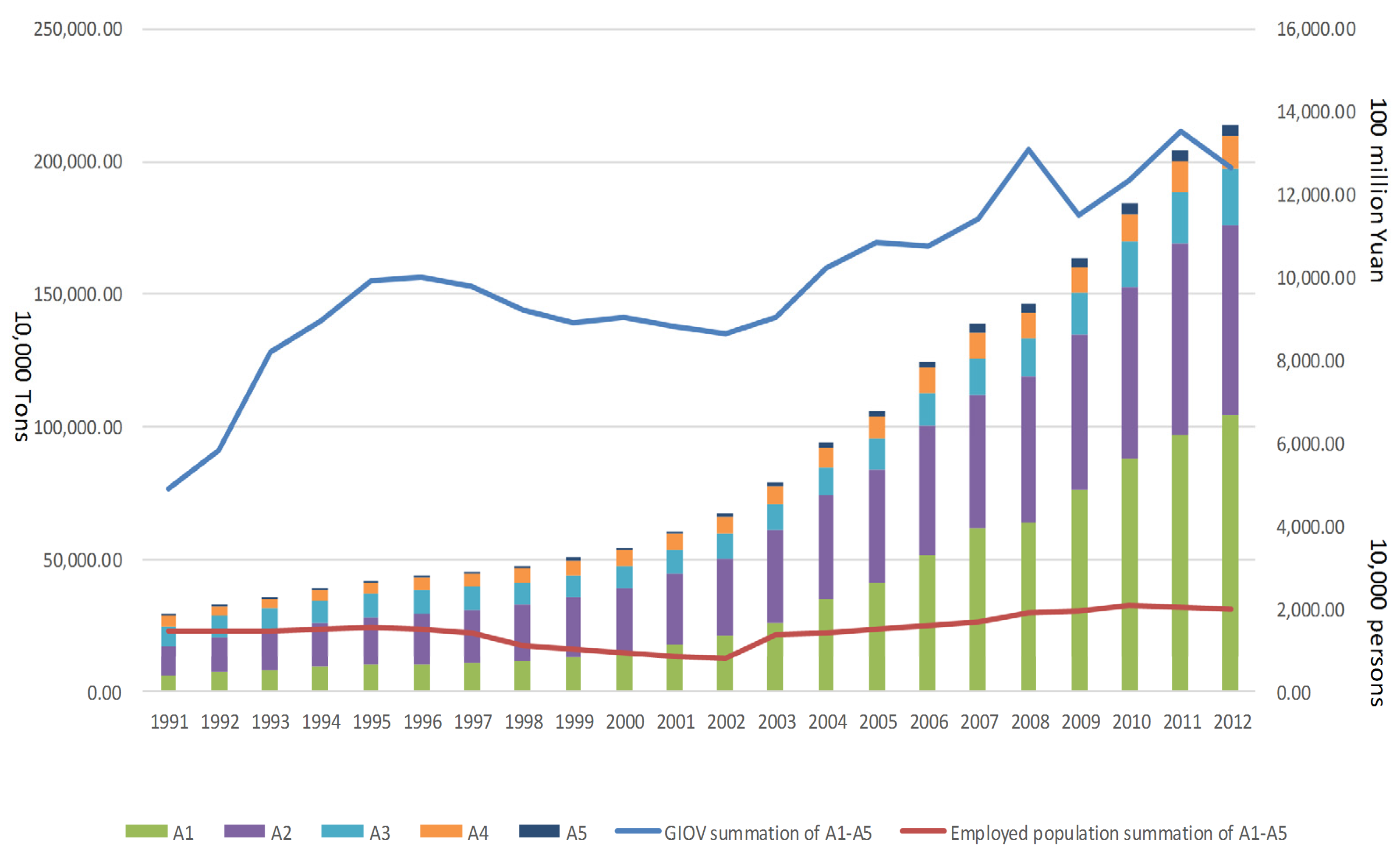
Table 3 also illustrates the employed population scale of each industrial department. It is important to note that the line chart in Figure 1 represents the gross value of industrial output at a constant price in 1990 (blue line) and industrial employed population (red line), the units are one hundred million yuan and ten thousand people.
Some conclusions can be drawn from Table 3 and Figure 1. In terms of the overall scale, the proportion of gross industrial output value and industrial employed population of the five major IPPU CO2 emissions departments is about 20% of the total, and remained stable for a generous portion of the time period. It is also determined by each IPPU CO2 emission department’s characteristic: they represent favorable industrial bases and facilities overall, both in basic manufacturing and mining departments, as far as ensuring stable development of the national economy and livelihood, and more stable product supply and marketing demand; thus, the proportion remains around 20% steadily.
From the overall view, CO2 emissions are determined by the product yield, so with the increase of product output, CO2 emissions rose and reached their maximum in 2012, 2142.3957 million tons, while the industrial department employed population and gross industrial output value firstly began to decline from 1996 to 2002 steadily and then increased after 2002. This is because, since 1998, China’s accumulation of deep-seated economic issues became problematic, and layoffs and unemployment became common social phenomena in China’s state-owned enterprises. In the middle of the 1990s, China experienced an economic recession characterized by lack of external or internal demand. The stagnation of the whole industry chain made all related enterprises face a very embarrassing situation. Large- and medium-sized, state-owned enterprises going bankrupt reduced the GIOV during this period; both reached their nadir in 2002, at 8.22 million (the total employed population in 2002 is 37.29 million) and 863.006 billion (the total China’s GIOV in 2002 is 4675.18 billion yuan), respectively. After 2002, with China’s accession to the WTO (World Trade Organization), a massive boom in domestic and foreign demand strengthened the economy and saved many state-owned enterprises from bankruptcy. Particularly, large state-owned enterprises like iron and steel producers began to make the transition from the planned economy to the market economy, ultimately rising to meet renewed external and internal demand. The industrial worker population and GIOV rose again; worker population peaked in 2010 at 21.0441 million (compared to the total population of China, 95.4471 million) and GIOV in 2011 at 1355.766 billion yuan (compared to the total gross value of China, 6,394.32 billion yuan), but, in 2011 and 2012, both values leveled off as the growth of the global economy slowed; this weakened external demand considerably, causing declining domestic infrastructure investment and weakening China’s real estate market regulations. These reasons sharply slowed down the speed of China’s economic growth, especially in manufacturing. Manufacturing’s employed demand growth slowed markedly while the construction, resident service and other services employed demand grew rapidly. As a result, the employment pressure will be more and more aggravated. In the next few years, China’s labor supply and structure will continue to change, the overall workforce will usher in a new turning point in a few years, and the new labor force and employed population will continue to decline among young adults. In the next few years, China’s labor supply and structure will certainly continue to change. New turning points in the country’s overall workforce are inevitable, including reducing the number of young adults employed in the industrial field. As the economy slows down and reaches stagnation, the employed population size will be stable.
From the view of the five major IPPU CO2 emission industrial departments, steel and iron alloy manufacturing, and non-metallic manufacturing accounted for more than 80% of total emissions, and reached 82.2% in 2012. With the increasing production of steel and cement, glass, CO2 emissions will continue to increase steadily over these years, while the rest of the industry growth rates are slower than A1 and A2. Taking the five major IPPU CO2 emission industrial departments as a whole, the steel and iron alloy manufacturing and chemical industry occupy nearly 60% of gross industrial output value, and non-metal and metal manufacturing industry occupies 20%. Non-metallic mining comprises the smallest portion at only about 2%. The non-metallic manufacturing industry, interestingly, shows the greatest proportion of the worker population at nearly 30%, while steel and iron alloy manufacturing and the metal industry comprises 19% and 11% of the worker population, respectively. The non-metallic mining worker population also presents a rising trend, from 7.7% in 1991 to 17.3% in 2012, while the chemical industry fell about 5% in 2012 in comparison to that of the 1990s. Due to the relative stability of China’s industrial development in recent years, the employed population structure also tends to be stable, both as a reflection of domestic and foreign demand characteristics. Due to the relative stability of China’s industrial development in recent years, the employed population structure also tends to be stable, both as a reflection of domestic and foreign demand characteristics. As China’s cement, glass, and iron alloy manufacturing industries are national leaders in production (and accordingly are top-priority infrastructure investment targets, demand-creators, and policy-drivers), the corresponding GIOV and employed population stayed at high levels toward the end of the time period we examined. The chemical industry and metal industry are pillars of China’s industrial infrastructure and effectively serve as the foundational livelihood of a massive employed population and of China’s economic and social stability—in short, no changes to this infrastructure can be expected in the short term. Non-metallic mining can be considered as a bottleneck industry, conversely. Due to its high dependence on natural resources, this industry tends to be more exploitative (i.e., its GIOV, in effect, inextricably corresponds to the exploitation and industrial pretreatment of its products.). Obviously, making any substantial increase in industrial output of this kind of resource-intensive industry is impossible in terms of environmental sustainability.

4.2. The Verification of IPPU CO2 Kuznets Curve

Upon testing, the time sequence series are consistent with cointegration test precondition. The result of the unit root test shows that the IPPU CO2 emissions of per employed person time series and the GIOV per employed person time series are both non-reposeful time series and integrated series of the first order. Then, taking the variable cointegration with the Johanse–Juselius test. The examination shows that the corresponding variable co-integration relationship exists as well. Therefore, scatter plot description and regression analysis can proceed.
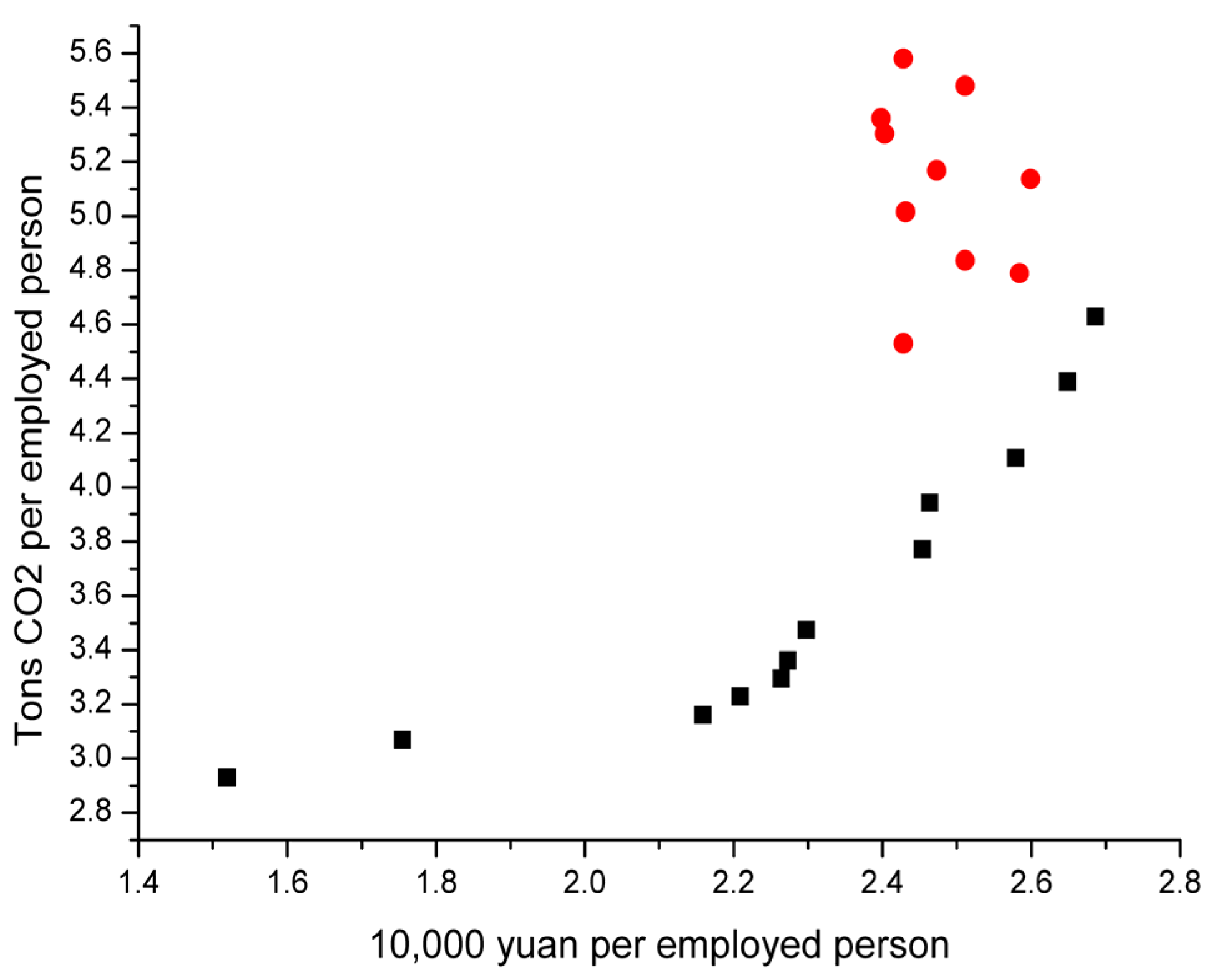
Figure 2, Figure 3, Figure 4, Figure 5, Figure 6 and Figure 7 shows the scatterplots of five major IPPU CO2 emissions departments as well as their summation. It can reflect the relationship between IPPU CO2 emissions per employed person and GIOV per employed person, as well as the change trend in both. The abscissa represents GIOV per employed person and the unit is ten thousand yuan. The ordinate represents the IPPU CO2 emissions per employed person, and the unit is tons. Natural logarithm processing has been done to all data.
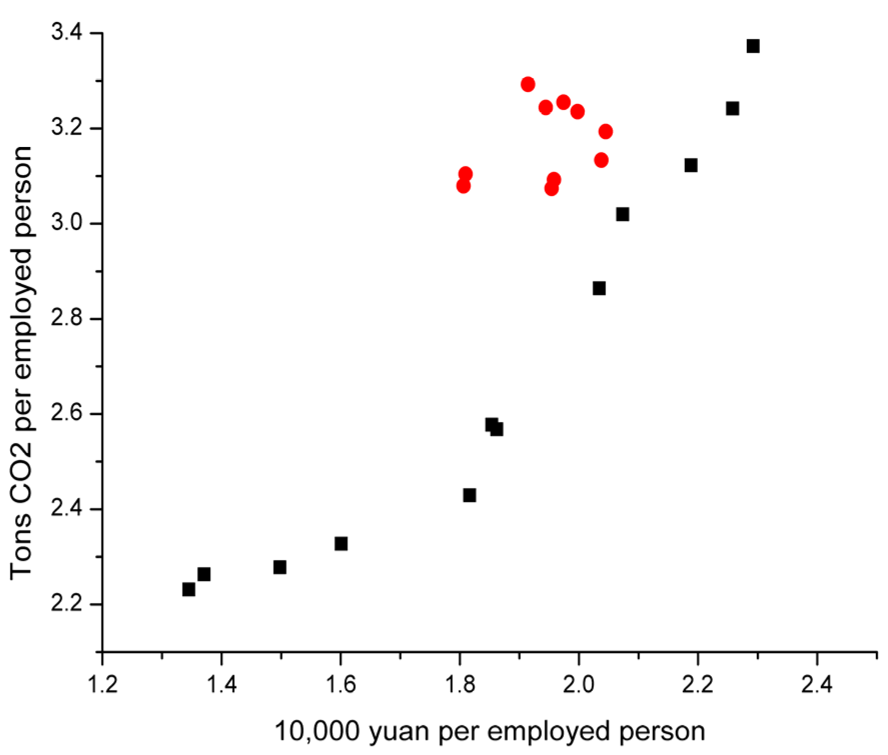
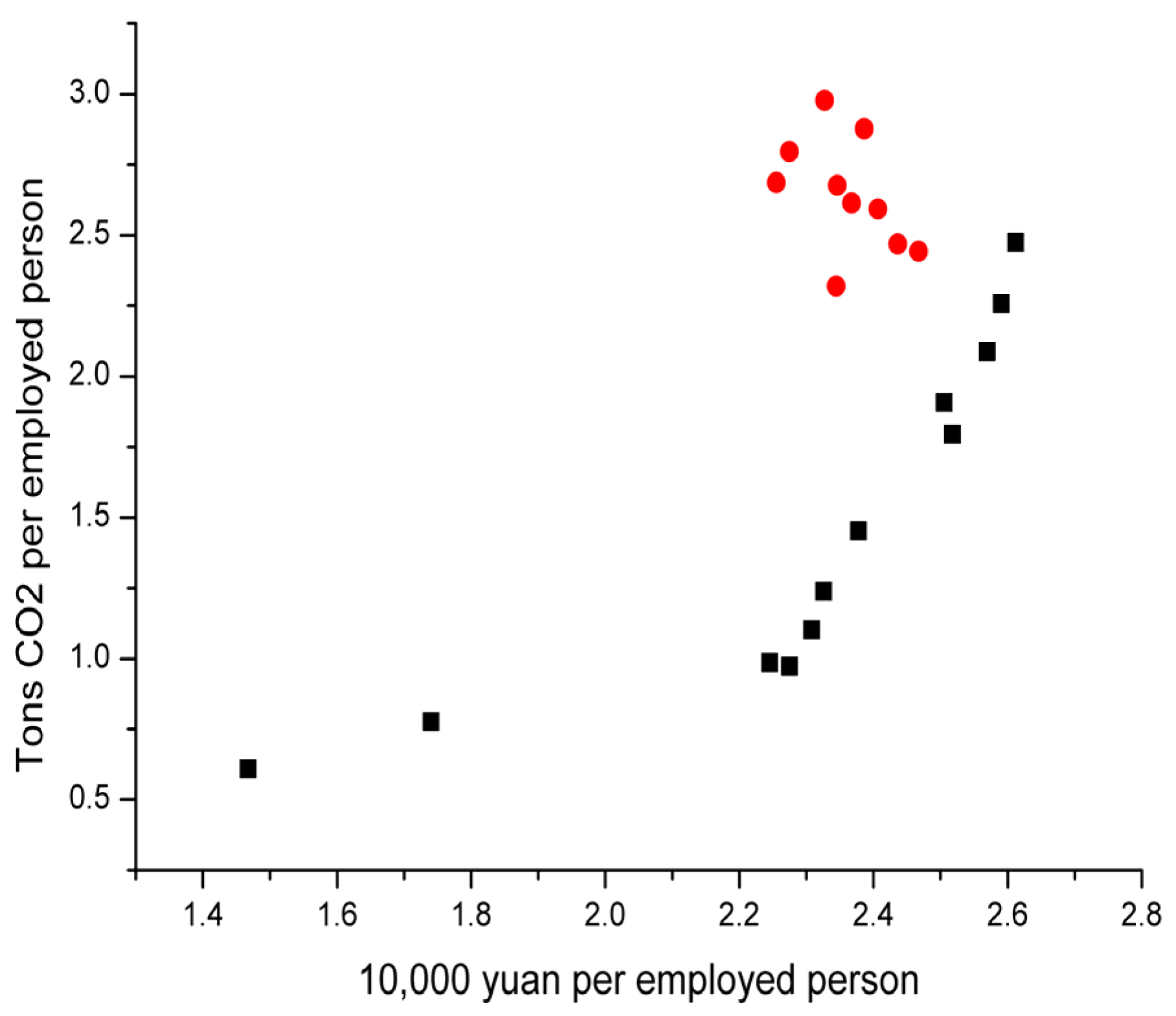
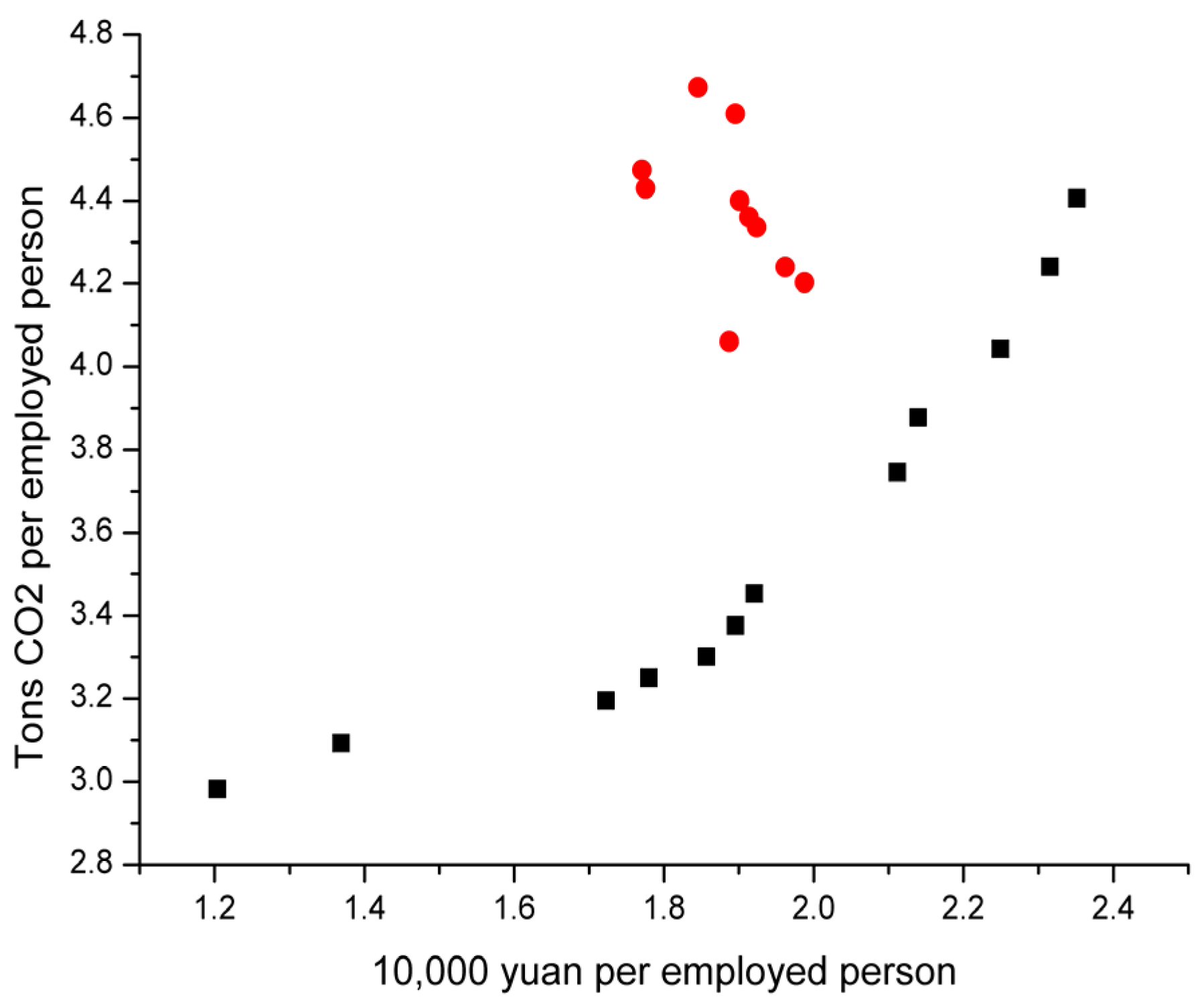
Unlike those drawn in previous studies, the scatter do not present any classic inverted U-shaped, N-shaped and other Kuznets curve types. Except non-metallic mining’s scatterplot presenting a function type growth curve, the rest of the IPPU department data are divisible into two parts marked with red and black splashes, respectively. The black scattered data represents 1991–2002 values which presented a function type growth curve and the red scattered data represents 2002–2012 values, which created a gathering type phenomenon, and all red scattered data are upper left of the black curve, namely GIOV per employed person value declined after 2002.
We consider non-metallic mining as a regression example in Table 4 because β3 is not significant in cubic form, while β2 is significant, so quadratic regression is adopted. Then, we checked the D.W. value to judge whether the regression residuals show series autocorrelation.
According to the result, D.W. = 0.498941 < DL = 0.9711, which indeed demonstrates autocorrelation between CO2 emissions and GIOV. Then, we added AR (AR(1) means the random disturbance is the first-order autoregressive form of serial correlation) to the estimating equations to eliminate autocorrelation sequence via the generalized least square method and obtain the results list in Table 5.
The final result (in which we took four decimal places, the same as the following regression analysis results):
ln P C A 3 = 4.0041 + 0.3829 ln P G I O V A 3 + 0.5338 ln 2 P G I O V A 3 + ε
The following regression analysis results can be obtained in Table 6 with the Generalized Least Squares. According to the results, estimate equation and the analysis of the results are shown as follows:
After obtaining the coefficient and the related parameters in the equation, due to the uncertainty of initial definition, diagnostic tests (tests on residuals, specification and stability tests and so on) of regression equations should be checked. In this paper, White heteroscedasticity testing, Chow breakpoint test, and Granger causality test are adopted from different perspectives. Consider the chemical industry as a regression example, and the results are as follows:
From the result in Table 7, F-statistic and the corresponding probability indicate that there is no heteroscedasticity in the residual and regression coefficient keeping stable at different times, PCA4 does not Granger Cause PGIOVA4 and PGIOVA4 does not Granger Cause PCA4.
Similarly, other industry departments and the total industrial department also carry out the diagnostic test and get the same conclusion. Because of the limitation of length, there is no more tautology here. Finally, the estimate equations are obtained in Section 4.2.1 to Section 4.2.6.

4.2.1. Steel and Iron Alloy Manufacturing

1991–2002
ln P C A 1 = 10.9220 8.6099 ln P G I O V A 1 + 2.3256 ln 2 P G I O V A 1 + ε
In 2002, PGIOVA1, PCA1 reached maximum, lnPGIOVA1 = 2.686, lnPCA1 = 4.629.
2003–2012
lnPGIOVA1 stays within the interval (2.398, 2.599). lnPCA1 began to rise resiliently in recent years after a slight decline, and reached the maximum, 5.581, in 2012.

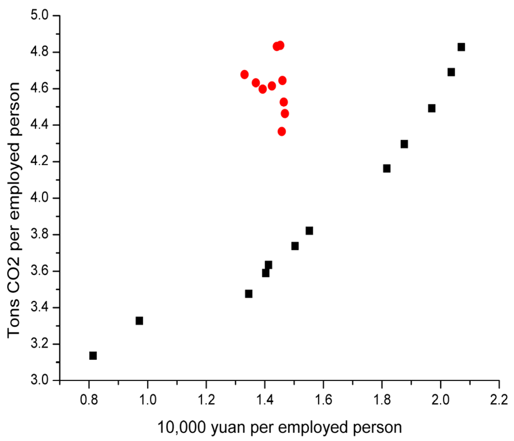
4.2.2. Non-Metallic Manufacturing

1991–2002
ln P C A 2 = 5.8212 3.6652 ln P G I O V A 2 + 1.5282 ln 2 P G I O V A 2 + ε
In 2002, PGIOVA2, PCA2 reached maximum, lnPGIOVA2 = 2.071, lnPCA2 = 4.828.
2003–2012
lnPGIOVA2 stays within the interval (1.331, 1.469). lnPCA2 began to rise resiliently in recent years after a slight decline, and reached its maximum, 4.837, in 2011. The value was 4.832 in 2012.

4.2.3. Non-Metallic Mining

1991–2012
ln P C A 3 = 4.0041 + 0.3829 ln P G I O V A 3 + 0.5338 ln 2 P G I O V A 3 + ε
In 2002, PGIOVA3, PCA3 reached the maximum of the whole time series from 1991 to 2012, lnPGIOVA3 = 1.066, lnPCA3 = 5.066. In fact, compared to the value in 2002, lnPGIOVA3 and lnPCA3 in 2003–2012 both showed a greater degree of decline and did not follow the increasing trend pre-2002, though the data do fall onto the overall fitting curve coincidentally.

4.2.4. Chemical Industry

1991–2002
ln P C A 4 = 4.6514 3.5199 ln P G I O V A 4 + 1.2920 ln 2 P G I O V A 4 + ε
In 2002, PGIOVA4, PCA4 reached maximum, lnPGIOVA4 = 2.292, lnPCA4 = 3.373.
2003–2012
lnPGIOVA4 stays within the interval (1.806, 2.045). lnPCA4 began to rise resiliently in recent years after a slight decline, and reached its maximum, 3.293, in 2012.

4.2.5. Metal Industry

1991–2002
ln P C A 5 = 12.7823 13.0570 ln P G I O V A 5 + 3.4722 ln 2 P G I O V A 5 + ε
In 2002, PGIOVA5, PCA5 reached maximum, lnPGIOVA5 = 2.612, lnPCA5 = 2.474.
2003–2012
lnPGIOVA5 stays within the interval (2.255, 2.467). lnPCA5 began to rise resiliently in recent years after a slight decline, and reached its maximum, 2.977, in 2012.

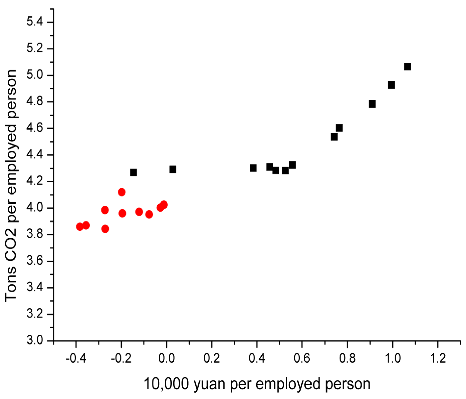
4.2.6. The Sum of the Five Major IPPU CO2 Emission Departments

1991–2002
ln P C A = 6.1980 4.4040 ln P G I O V A + 1.5409 ln 2 P G I O V A + ε
In 2002, PGIOVA, PCA reached its maximum, lnPGIOVA = 2.351, lnPCA = 4.405.
2003–2012
lnPGIOVA stays within the interval (1.771, 1.988). lnPCA began to rise resiliently in recent years after a slight decline, and reached its maximum, 4.673, in 2012.
Compared with the previous studies on industry EKC, the source of basic data and curve shape are not the same for several situations, but the vast majority of the carbon emission data are from the energy consumption [11,12,15,16], there is almost no carbon emissions EKC analysis caused by industrial production process. On the other hand, from the point of curve shape, although the curve shapes exist in a variety of forms [3,4,5,6,7,8,9,10,14,15,16], the two obvious parts of the scatters have never appeared before. This paper focused on the relationship between industry CO2 emissions and economic activity, and CO2 emissions are accounted for in terms of IPPU rather than energy consumption. Though the surface result is similar with the research [10,16] that an inverted-U EKC does not exist, due to the IPPU CO2 data the first time, our novel use of IPPU CO2 data made our scatter and regression analysis quite different from those of previous researchers. Because of the data result accounting and the curve fitting situation, a new relationship between IPPU CO2 emission and GIOV is put forward for the first time in this paper. The reasons and discussions are as follows.
Prior to 2002, reduction in domestic and foreign demand caused either stagnation or decline in China’s manufacturing sector overall (including the steel, cement, glass, and chemical industries) as well as a decline in the GIOV as prices remained constant and employed population declined, while the decreasing amount is far from the range of laid-off and unemployed workers. Several of China’s state-owned enterprises reduced surplus staff during this time in effort to prevent bankruptcy, maintain (low) production levels, and avoid collapse exponentially of the employed population. This caused the ascendant trend in the GIOV per employed curve.
After 2002, with China’s accession to the WTO, the increasing domestic and foreign demand and widespread new construction of domestic infrastructures required a larger workforce; accordingly, the population of employed persons increased yearly from this point forward. The economic growth rate also tended to be stable in those years, though it grew at a slower rate than that of the worker population. To this effect, the GIOV per worker data moved to the left of the black curve after 2002. After 2010, China’s labor force structure was fairly stable, and the number of workers was around 90 million. As-affected by a sluggish global economy, weakened external demand, slowed domestic infrastructure investment, new real estate market regulations, and other factors, China’s economic growth then slowed down (especially in terms of manufacturing growth rate). The GIOV stalled once again while the GIOV per worker remained unchanged, dropping below the maximum in 2002.
The production increase is related to domestic and foreign demand directly working on increasing CO2 emissions; likewise, emissions decline when production declines. After 2002, IPPU CO2 emissions per employed person in all departments presented a slight decline in 2003, followed by an overall increase until reaching maxima in 2011 and 2012. Among the separate curves for individual department, steel and iron alloy manufacturing and metal industry IPPU CO2 emissions per employed person reached its maximum in 1991–2012, while the remaining departments’ extremum values were slightly smaller than that of the 2002 maximum.
GIOV is affected by the apparent output consumption data accounted in this paper by IPPU CO2 emission, and there was a greater distance between data points in 2003 to 2012 and the fitting curve in 1991–2012 that reflects the greater difference between product output and consumption. Take the iron and steel industry for example, before 2003, China’s steel industry was in short supply and domestic production did not meet the needs of economic development, but, after 2003, with the capacity of expanding and enterprise’s production enthusiasm, the iron and steel industry appeared in the steel stocks. As the economy gradually stabilized over these years, the overcapacity problem got worse noticeably. In 2012, the difference between demand and supply reached its maximum, nearly 300 million tons, and its reflective phenomenon reflects the scatter performance.
In fact, the calcium carbide and lime mining also complies with the principle of the above. In 2002, lnPCA3 and lnPGIOVA3 reached the maximum, then it dipped to a low level.
The scatter we created for the summation of all five major IPPU CO2 emission departments was similar to that of individual manufacturing sectors (apart from that of non-metallic mining, which was quite a bit smaller and had fewer effects on the whole). In 2002, the GIOV per employed person value reached its maximum and then began to decline, as discussed above. The IPPU CO2 emissions per employed person rose slightly after a slight decline in 2002, then reached its maximum in 2012.
According to the classic Kuznets curve theory, carbon emissions and economic growth present the inverted U-shaped curve. However, in this paper, the results show a weaker relationship between IPPU CO2 emissions per worker and GIOV per worker (i.e., two different curve shapes) in terms of IPPU CO2 emissions. These scatterplots may provide a valuable reference for future policy adjustments made to the industrial sector as well.
Especially the data since 2003, which moved to the left above the curve in 1991-2002, the per capita CO2 emissions presents an increasing trend in recent years and reached the maximum in 2011 or 2012. This reflects a serious circumstance: due to small changes in GIOV and the employed population, China’s iron and steel, cement and other industries demand have tended to become saturated and even reduced. While the production is still increasing, the problem of excess production capacity has appeared in China in recent years, and a worsening overcapacity situation has been alarming the government.

5. Conclusions

Based on IPPU CO2 emissions calculating equations in IPCC 2006, this paper preliminarily calculated and established a time series for China’s IPPU CO2 emissions in 1991-2012. Combined with the GIOV and employed population, this paper analyzed the relationship between IPPU CO2 emissions level and industrial economic development, and reached some interesting conclusions.
The overall trend shows that CO2 emissions are determined by the product yield. CO2 emissions increased until reaching a maximum in 2012; the IPPU CO2 emissions related to the employed population and GIOV first steadily declined from 1996 to 2002, then increased from 2002 to the end of the observed time period. Steel and iron alloy manufacturing and non-metallic manufacturing CO2 emissions accounted for more than 80% of total emissions, and up to 82.2% in 2012. The steel and iron alloy manufacturing and chemical industry occupied nearly 60% of GIOV, while non-metal and metal manufacturing industries occupied 20%, and non-metallic mining are only 2%. The non-metallic manufacturing industry had the greatest proportion of the employed population, however, at nearly 30%.
The curves we drew to represent the relationship between GIOV and IPPU CO2 emissions marked a departure from Kuznets curves in previous studies: The scatterplots did not present any classic inverted U-shaped or N-shaped curves. Most of the industrial department (except non-metallic mining) and the sum of all sectors presented two-part curves. Before 2002, the data formed a quadratic or a cubic function curve, and after 2003, GIOV per employed person remained within a certain range while IPPU CO2 emissions per worker fell slightly, then continued to rise gradually.
According to the current situation of economic and employment, it is impossible for large-scale industrial economy to grow and the employed population to change. Therefore, decreasing CO2 emission intensity and per capita indicators should come directly from the CO2 emission source—IPPU. The government should design policy measures from the perspective of the removal of excess capacity and elimination of backward production capacity, namely, reducing new production capacity, repeated use of products whenever possible, and replacing outdated equipment to reduce carbon emissions. Certain processes, such as those practiced in the non-metallic mining industry, metal industry, and chemical industry are unitary and stable and they create only relatively low IPPU CO2 emissions, while steel and cement manufacturing are primary culprits of high IPPU CO2 emissions as well as industries that are traditionally vulnerable to overcapacity. It is absolutely imperative to cut down the CO2 emissions from these two industries.
The most direct path for the cement industry is to reduce production, use up current inventory and extend the service life of cement materials. On one hand, carbonate decomposition can produce a massive amount of CO2 emissions; thus, blasting furnace slag, fly ash and other industrial waste instead of carbonate can be used to reduce IPPU CO2 significantly. In addition, mixed material and mineralizing agent can be applied to the cement clinker production process as well. On the other hand, to improve the cement performance, which would improve the material’s service life, would reduce demand for cement as well. There has been a similar situation in steel and iron alloy products, and some areas’ production has already met the needs of the next 10 years. Reducing production, using up inventory, and smelting scrap steel are the most direct paths to sustainability. A transition to the electric arc furnace could substantially reduce the IPPU values of the steel and iron alloy industries. Though most open-hearth steelmaking production has been eliminated, there is much work yet to be done to make these industries environmentally sustainable. Because the current cement industry and iron and steel industry have gone into a downturn, and there has been no mass production or demand of steel and cement possible in recent years due to the depressed market, it is a golden age to make the scatter return to more normal levels by digesting inventory and adjusting the technology structure. If steel and cement industries do not take advantage of the depressed market situation now and do not adjust structure quickly, the future to reduce the IPPU CO2 emission will be a more serious issue while the rapid economic development appears once again.
Though current IPPU carbon emissions and corresponding GIOV do not show a Kuznets curve, they do indeed show rising trends. The top five industries examined in this study comprise about 20% of China’s total GIOV, reflecting that they are pillars of the country’s economy and central to the livelihood of millions of workers, meaning that substantive changes to infrastructure in the short term are effectually impossible. Instead, promoting investment in industrial capital and equipment is imperative to the technological improvement necessary for environmental sustainability. Improving R & D efficiency to raise product quality, eliminating production of low output value materials, and minimizing energy consumption are also effective paths to a two-fold goal of ensuring valuable products and a healthy economy while ensuring the stable livelihood of the workforce. In effect, sustainability measures can improve the value of GIOV per employed person in China, ushering China into a new era of economic and environmental sustainability.

Acknowledgments

The authors gratefully acknowledge the financial support from the National Natural Science Foundation of China (71273039). This research has also been supported by the Key Laboratory of Ocean Energy Utilization and Energy Conservation of Ministry of Education, the Fundamental Research Funds for the Central Universities (DUT14RC(3)151) and the China Postdoctoral Science Foundation (2015M571309).

Author Contributions

Both authors contributed equally to this work. In particular, Hailin Mu and Ye Duan had the original idea for the study, and both coauthors conceived of and designed the methodology. Ye Duan drafted the manuscript, which was revised by Hailin Mu and Nan Li. All authors have read and approved the final manuscript.

Conflicts of Interest

The authors declare no conflict of interest.

References

  1. Grossman, G.M.; Krueger, A.B. Environmental Impacts of a North American Free Trade Agreement; Working Paper No. 3914; National Bureau of Economic Research: Cambridge, UK, 1991; pp. 1–37. [Google Scholar]
  2. Shafik, N. Economic development and environmental quality: An econometric analysis. Environ. Econ. 1994, 46, 757–773. [Google Scholar]
  3. Hettige, H.; Lucas, R.E.B.; Wheeler, D. The toxic intensity of industrial production; global patterns, trends, and trade policy. Am. Econ. Rev. 1992, 82, 478–481. [Google Scholar]
  4. Selden, T.M.; Song, D. Environmental quality and development: Is there a Kuznets curve for air pollution emissions? J. Environ. Econ. Manag. 1994, 27, 147–162. [Google Scholar] [CrossRef]
  5. Grossman, G.M.; Krueger, A.B. Economic growth and the environment. Q. J. Econ. 1995, 110, 353–377. [Google Scholar] [CrossRef]
  6. Hill, R.J.; Magnani, E. An exploration of the conceptual and empirical basis of the environmental Kuznets curve. Aust. Econ. Pap. 2002, 42, 239–254. [Google Scholar] [CrossRef]
  7. Stem, D.L. The rise and fall of the environmental Kuznets curve. World Dev. 2004, 32, 1419–1439. [Google Scholar]
  8. Lantz, V.; Feng, Q. Assessing Income, Population and technology impacts on CO2 emissions in Canada: Where’s the EKC? Ecol. Econ. 2006, 57, 229–238. [Google Scholar] [CrossRef]
  9. Ranjan, R.; Shortle, J. The environmental Kuznets curve when the environment exhibits hysteresis. Ecol. Econ. 2007, 64, 204–215. [Google Scholar] [CrossRef]
  10. He, X.; Zhang, Y. Influence Factors and Environmental Kuznets Curve Relink Effect of Chinese Industry’s Carbon Dioxide Emission—Empirical Research Based on STIRPAT Model with Industrial Dynamic Panel Data. China Ind. Econ. 2012, 1, 26–35. [Google Scholar]
  11. Lu, H. An Analysis on China’s Economy Development and on State space Model of Environment—Take Air Pollution as an Example. Study Financ. Econ. 2000, 26, 53–59. [Google Scholar]
  12. Cai, F.; Du, Y.; Wang, M. The Political Economy of Emission in China: Will a Low Carbon Growth Be Incentive Compatible in Next Decade and Beyond? Econ. Res. J. 2008, 6, 4–11. [Google Scholar]
  13. Huang, W.M.; Lee, G.W.M.; Wu, C.C. GHG Emissions, GDP Growth and the Kyoto Protocol: A Revisit of Environmental Kuznets Curve Hypothesis. Energy Policy 2008, 36, 239–247. [Google Scholar] [CrossRef]
  14. Han, Y.; Lu, Y. The Relationship between Economic Growth and Environmental Quality: An Empirical Test on the Environmental Kuznets Curve of CO2. Econ. Theory Bus. Manag. 2009, 3, 5–12. [Google Scholar]
  15. Zheng, L.; Zhu, Q. Study on Existence of Environmental Kuznets Curve of Carbon Emissions in China. Stat. Res. 2012, 29, 58–65. [Google Scholar]
  16. Zhang, M. Measurement of Carbon Emission in the Manufacturing Segmented Industry of China-Giving Discussion of the Existence of EKC in the Manufacturing Industry. Soft Sci. 2015, 29, 113–116. [Google Scholar]
  17. Dorel, P.; Cristiana, T.; Radu, P. The Textile Industry and Sustainable Development: A Holt-Winters Forecasting Investigation for the Eastern European Area. Sustainability 2015, 7, 1280–1291. [Google Scholar]
  18. Valentina, D.; Battista, G.; Giorgio, M. Environmental Sustainability of the Alumina Industry in Western Europe. Sustainability 2014, 6, 9477–9493. [Google Scholar]
  19. Van Puyvelde, D. CCS opportunities in the Australian Industrial Processes sector. Energy Procedia 2009, 1, 109–116. [Google Scholar] [CrossRef]
  20. Sheinbaum, C.; Ozawa, L.; Castillo, D. Using logarithmic mean divisia index to analyze changes in energy use and carbon dioxide emissions in Mexico’s iron and steel industry. Energy Econ. 2010, 32, 1337–1344. [Google Scholar] [CrossRef]
  21. Arruda, L.R.; de Jesus Lameira, V.; Quelhas, O.L.G.; Pereira, F.N. Sustainability in the Brazilian Heavy Construction Industry: An Analysis of Organizational Practices. Sustainability 2013, 5, 4312–4328. [Google Scholar] [CrossRef]
  22. Liaskas, K.; Mavrotas, G.; Mandaraka, M.; Diakoulaki, D. Decomposition of industrial CO2 emissions: The case of European Union. Energy Econ. 2000, 22, 383–394. [Google Scholar] [CrossRef]
  23. Kim, Y.; Worrell, E. International comparison of CO2 emission trends in the iron and steel industry. Energy Policy 2002, 30, 827–838. [Google Scholar] [CrossRef]
  24. Kirschen, M.; Risonarta, V.; Pfeifer, H. Energy efficiency and the influence of gas burners to the energy related carbon dioxide emissions of electric arc furnaces in steel industry. Energy 2009, 34, 1065–1072. [Google Scholar] [CrossRef]
  25. Zhou, W.; Zhu, B.; Li, Q.; Ma, T.; Hu, S.; Griffy-Brown, C. CO2 emissions and mitigation potential in China’s ammonia industry. Energy Policy 2010, 38, 3701–3709. [Google Scholar] [CrossRef]
  26. Dong, X.; Guo, J.; Höök, M.; Pi, G. Sustainability Assessment of the Natural Gas Industry in China Using Principal Component Analysis. Sustainability 2015, 7, 6102–6118. [Google Scholar] [CrossRef]
  27. Liu, W.; Wu, X.; Ding, X. Industrial carbon footprint calculation of woolen yarn. Wool Text. J. 2015, 2, 57–61. [Google Scholar]
  28. Liu, Z.; Dong, H.; Geng, Y.; Lu, C.; Ren, W. Insights into the Regional Greenhouse Gas (GHG) Emission of Industrial Processes: A Case Study of Shenyang, China. Sustainability 2014, 6, 3669–3685. [Google Scholar] [CrossRef]
  29. Gao, J.; Wang, Y.; Li, Q. Estimation on Carbon Emissions from Fossil Fuel and Industrial Production from 2000 to 2009 in Henan Province. Territ. Nat. Resour. Study. 2011, 5, 48–50. [Google Scholar]
  30. Chen, H. Analysis on Embodied CO2 Emissions Including Industrial Process Emissions. China Popul. Resour. Environ. 2009, 19, 25–30. [Google Scholar]
  31. IPCC. IPCC Guidelines for National Greenhouse Gas Inventories; United Kingdom Meteorological Office: Bracknell, UK, 2006. [Google Scholar]
  32. CSY. China Statistical Yearbook; National Bureau of Statistics of the People’s Republic of China: Beijing, China, 1991–2012.
  33. NBS. China Compendium of Statistics 1949–2008; National Bureau of Statistics of the People’s Republic of China: Beijing, China, 2010.
  34. CIESY. China Industrial Economy Statistical Yearbook, 1991–2012; National Bureau of Statistics of the People’s Republic of China: Beijing, China, 1991–2012.
  35. CCIY. China Chemical Industrial Yearbook, 1991–2012; National Bureau of Statistics of the People’s Republic of China: Beijing, China, 1991–2012.
  36. NBS. The Yearbook of Nonferrous Metals Industry of China, 1991–2012; National Bureau of Statistics of the People’s Republic of China: Beijing, China, 1991–2012.
Figure 1. IPPU CO2 emissions from A1–A5, Gross value of industrial output and industrial employed population.
Sustainability 08 00426 g001
Figure 2. Scatterplots of CO2 emissions and GIOV in steel and iron alloy manufacturing.
Sustainability 08 00426 g002
Figure 3. Scatterplots of CO2 emissions and GIOV in non-metallic manufacturing.
Sustainability 08 00426 g003
Figure 4. Scatterplots of CO2 emissions and GIOV in non-metallic mining.
Sustainability 08 00426 g004
Figure 5. Scatterplots of CO2 emissions and GIOV in the chemical industry.
Sustainability 08 00426 g005
Figure 6. Scatterplots of CO2 emissions and GIOV in the metal industry.
Sustainability 08 00426 g006
Figure 7. Scatterplots of CO2 emissions and GIOV in the sum of the five major IPPU CO2 emission departments.
Sustainability 08 00426 g007
Table 1. Notations and explanations used in this paper.
NotationsExplanations
tIPPU CO2 emissions industrial department
PCIPPU CO2 emissions per employed person
αThe intercept term
GIOVGross industrial output value
PGIOVGross industrial output value per employed person
βThe estimated parameter of PGIOV
εThe estimated residuals
Table 2. CO2 emission coefficient about involved IPPU departments in IPCC 2006.
No.DepartmentCoefficient of Carbon Emissions 104 t CO2/104 t Product
CO2aSteel65% BOF, 30% EAF, 5% OHF, and the coefficient is 1.46, 0.08, 1.72
CO2bCement0.55536
CO2cLime0.683
CO2dCalcium carbide1.154
CO2eGlass0.2
CO2fSynthesis ammonia1.694
CO2gSodium carbonate0.138
CO2hFerrosilicon4.38
CO2iManganese-silicon1.4
CO2jLead(Pb)0.52
CO2kMagnesium(Mg)3
CO2lZinc(Zn)1.72
CO2mVirgin aluminum1.69
CO2nLubricating grease0.2
CO2oUrea0.733
CO2pTitanium dioxide1.4
CO2qEthylene1.73
CO2rMethyl alcohol0.67
Table 3. Gross value of industrial output, IPPU CO2 emissions and industrial employed population.
The Gross Value of Industrial Output at Constant Price in 1990, One Hundred Million Yuan
Gross Value of Industrial Output Valued in ChinaA1A2A3A4A5Sum of A1–A5Sum of A1–A5 Accounted for the Proportion of the Total
199125,407.671525.041040.2697.691527.82698.424889.219.24%
199228,817.791989.281226.23115.151606.73911.905849.320.30%
199335,734.053127.201751.05164.431740.091410.508193.322.93%
199442,702.203351.671884.13176.932008.061539.358960.220.98%
199549,064.823541.452004.71188.252534.171639.189907.820.19%
199650,487.703476.702090.92196.352620.331648.0310,032.319.87%
199750,336.243395.532082.55195.562502.421638.939814.9919.50%
199848,272.453165.722011.75188.912324.751538.359229.4819.12%
199947,113.913031.521965.48184.572243.381470.298895.2418.88%
200048,433.103125.461957.61183.832265.811501.799034.5118.65%
200147,803.473081.711900.84178.502200.101480.778841.9218.50%
200246,751.803006.821855.98174.292148.181444.798630.0618.46%
200347,827.093211.281898.67178.302197.591543.039028.8718.88%
200450,744.543849.411966.44188.712422.181830.2810,257.020.21%
200553,231.024041.591994.89206.352627.581973.3110,843.720.37%
200654,827.953881.472026.83211.512638.102021.4310,779.319.66%
200756,527.624192.592056.89218.072738.342208.0111,413.920.19%
200860,428.035044.222225.95242.013044.762547.3613,104.321.69%
200957,164.914207.092218.45236.792681.522171.4911,515.420.14%
201060,308.984538.662274.58251.942896.042401.7412,363.020.50%
201163,943.204990.762438.76274.913178.752674.4913,557.721.20%
201262,856.174460.672417.50284.253051.602458.3412,672.720.16%
The IPPU CO2 Emissions, Ten Thousand Tons
Total EmissionsA1A2A3A4A5
199128,932.766255.3410,608.978066.383705.85296.22
199232,793.397403.0012,931.858187.933922.90347.71
199335,702.328517.3514,741.268265.233795.12383.35
199438,973.089291.0516,763.398330.014151.74436.89
199541,984.709929.3218,470.318417.364677.05490.66
199644,110.3210,323.5019,519.438405.515307.18554.70
199745,423.1011,017.7620,132.618463.075159.83649.83
199847,296.8811,807.8721,003.498408.295330.88746.35
199950,568.3513,296.0922,098.148592.425773.38808.32
200054,336.9114,419.7824,386.678838.465765.77926.23
200160,625.8117,573.4227,009.099100.935882.811059.56
200267,319.0520,985.8529,238.139508.616328.021258.43
200379,354.0426,314.3234,753.2210,046.856733.921505.72
200493,941.4634,932.7439,289.8910,689.677244.041785.12
2005105,843.6741,318.7342,608.9111,592.528285.952037.56
2006124,577.6851,431.7048,948.6812,670.039093.122434.16
2007138,898.1362,057.7249,995.3513,913.119859.333072.61
2008146,197.0463,801.3254,858.1314,815.039465.803256.75
2009163,610.3476,558.8457,944.4916,187.729578.133341.15
2010184,558.6087,784.0864,639.7917,523.6210,566.394044.72
2011204,635.7497,243.0771,953.2419,412.6411,659.414367.38
2012214,239.57104,330.2471,755.5821,336.4512,107.134710.17
The Industrial Employed Population, 10,000 persons
The Industrial Employed Population in ChinaA1A2A3A4A5Sum of A1–A5Sum of A1–A5 Accounted for the Proportion of the Total
19916551.00334.00461.00113.00398.00161.001467.0022.39%
19926621.00344.00464.00112.00408.00160.001488.0022.47%
19936626.00361.00456.00112.00389.00145.001463.0022.08%
19946580.00368.00463.00112.00405.00163.001511.0022.96%
19956610.00368.00488.00116.00412.00163.001547.0023.40%
19966450.00358.00465.00116.00407.00161.001507.0023.36%
19976215.00341.00441.00112.00392.00152.001438.0023.14%
19984753.00272.00327.0090.00304.00124.001117.0023.50%
19994428.00258.00301.0086.00282.00120.001047.0023.64%
20004102.00237.00273.0074.00254.00115.00953.0023.23%
20013838.00218.00248.0066.00230.00111.00873.0022.75%
20023729.00205.00234.0060.00217.00106.00822.0022.04%
20035748.57283.30441.83183.40311.33147.971367.8323.79%
20046098.62290.63452.67191.07315.66155.221405.2523.04%
20056895.96328.08461.14222.76339.99172.611524.5822.11%
20067358.43341.40470.59238.68357.78182.131590.5821.62%
20077875.20353.57495.03265.06380.28211.381705.3221.65%
20088837.63375.02552.96317.35429.64238.711913.6821.65%
20098831.22380.50564.02337.95440.49227.681950.6422.09%
20109544.71412.67601.15369.46474.14246.992104.4122.05%
20119167.29405.12570.56360.90454.86245.992037.4322.22%
20129095.21393.33572.17346.42449.78239.842001.5422.01%
Table 4. Cubic form and quadratic form regression in non-metallic mining.
VariableCoefficientStd. Errort-StatisticProb.
Cubic Form
C4.10999920.035799114.80810.0000
X0.4126770.0874794.7174690.0002
X2−0.3860250.329525−1.1714590.2567
X30.8014380.2953412.7136040.0142
Quadratic Form
C4.0461760.031185129.74690.0000
X0.4065030.1010384.0232750.0007
X20.4440540.1415753.1365200.0054
Table 5. Regression result using the generalized least square in non-metallic mining.
VariableCoefficientStd. Errort-StatisticProb.
C4.0040830.04146596.565480.0000
X0.3829220.1355332.8253040.0117
X20.5337740.1539563.4670470.0029
AR(1)0.6070730.1705613.5592660.0024
R2Adjusted R2S.D. Dependent VarF-StatisticD.W.
0.9726550.9678290.356543201.56121.422968
Table 6. Regression analysis results of the IPPU CO2 emissions departments.
Steel and Iron Alloy Manufacturing
VariableCoefficientStd. Errort -StatisticProb.
C10.921991.03050410.598690.0000
X−8.6099460.91443959.4155450.0000
X22.3255600.20142411.545600.0000
AR(1)50.3353050.28326251.1837270.2752
R2Adjusted R2S.D. Dependent VarF-StatisticD.W.
0.9900740.9858200.529344232.73952.247248
Non-Metallic Manufacturing
VariableCoefficientStd. Errort-StatisticProb.
C5.8212010.40826014.2585550.0000
X−3.6651950.462456−7.9254940.0001
X21.5282150.13483411.334060.0000
AR(1)0.5160230.0595998.6582050.0001
R2Adjusted R2S.D. Dependent VarF-StatisticD.W.
0.9976920.9967030.5146861008.5911.807023
Non-Metallic Mining
VariableCoefficientStd. Errort-StatisticProb.
C4.0040830.04146596.565480.0000
X0.3829220.1355332.8253040.0117
X20.5337740.1539563.4670470.0029
AR(1)0.6070730.1705613.5592660.0024
R2Adjusted R2S.D. Dependent VarF-StatisticD.W.
0.9726550.9678290.356543201.56121.422968
Chemical Industry
VariableCoefficientStd. Errort-StatisticProb.
C4.6514130.8532225.4515850.0010
X−3.5199160.934448−3.7668410.0070
X21.2919680.2510705.1458450.0013
AR(1)0.1178170.3784530.3113130.7646
R2Adjusted R2S.D. Dependent VarF-StatisticD.W.
0.9855670.9793820.406903159.33561.907908
Metal Industry
VariableCoefficientStd. Errort-StatisticProb.
C12.782291.17780810.852610.0000
X−13.057011.074519−12.151490.0000
X23.4721810.24266014.308860.0000
AR(1)−0.4150510.204208−2.0324880.0816
R2Adjusted R2S.D. Dependent VarF-StatisticD.W.
0.9895750.9851070.581921221.48712.100003
The Sum of the 5 Major IPPU CO2 Emission Departments
VariableCoefficientStd. Errort-StatisticProb.
C6.1980140.40853215.171410.0000
X−4.4040280.429709−10.248870.0000
X21.5409280.11152713.816640.0000
AR(1)−0.2963030.302890−0.9782510.3605
R2Adjusted R2S.D. Dependent VarF-StatisticD.W.
0.9961640.9944940.452141603.10672.482855
Table 7. White Heteroskedasticity Test, Chow Breakpoint Test, Granger Causality Test in Chemical Industry.
White Heteroskedasticity Test
F -StatisticProb.Obs R2Prob.
1.2562140.32083.8106240.2827
Chow Breakpoint Test: 1997 (Other Hypothetical Breakpoint Dates Have the Same Conclusion)
F-Statistic0.851206Prob.0.5087
Granger Causality Test, Lags = 2
PCA4 does not Granger Cause PGIOVA4F-Statistic0.36198Prob.0.7132
PGIOVA4 does not Granger Cause PCA41.078850.4078

