Article

Predicting China’s SME Credit Risk in Supply Chain Financing by Logistic Regression, Artificial Neural Network and Hybrid Models

1
College of Business Administration, Hunan University, Changsha 410082, China
2
Center of Finance and Investment Management, Hunan University, Changsha 410082, China
3
Economics and Management School, Wuhan University, Wuhan 430072, China
4
China Huarong Asset Management CO., LTD., Beijing 100033, China
*
Author to whom correspondence should be addressed.
Sustainability 2016, 8(5), 433; https://0-doi-org.brum.beds.ac.uk/10.3390/su8050433
Submission received: 18 February 2016 / Revised: 22 April 2016 / Accepted: 26 April 2016 / Published: 3 May 2016
(This article belongs to the Section Economic and Business Aspects of Sustainability)

Abstract

:
Based on logistic regression (LR) and artificial neural network (ANN) methods, we construct an LR model, an ANN model and three types of a two-stage hybrid model. The two-stage hybrid model is integrated by the LR and ANN approaches. We predict the credit risk of China’s small and medium-sized enterprises (SMEs) for financial institutions (FIs) in the supply chain financing (SCF) by applying the above models. In the empirical analysis, the quarterly financial and non-financial data of 77 listed SMEs and 11 listed core enterprises (CEs) in the period of 2012–2013 are chosen as the samples. The empirical results show that: (i) the “negative signal” prediction accuracy ratio of the ANN model is better than that of LR model; (ii) the two-stage hybrid model type I has a better performance of predicting “positive signals” than that of the ANN model; (iii) the two-stage hybrid model type II has a stronger ability both in aspects of predicting “positive signals” and “negative signals” than that of the two-stage hybrid model type I; and (iv) “negative signal” predictive power of the two-stage hybrid model type III is stronger than that of the two-stage hybrid model type II. In summary, the two-stage hybrid model III has the best classification capability to forecast SMEs credit risk in SCF, which can be a useful prediction tool for China’s FIs.

1. Introduction

Intense market competition, capital shortages and globalization generate complex and dynamic supply chains. Reinforcing the management of material flow and information flow does not necessarily result in improving the management of supply chain. Therefore, the focus of supply chain management today is on the design and optimization of cash flow [1]. Supply chain financing (SCF) has increasingly become a hot topic in supply chain management and a growing product category of financial institutions (FIs). In China, SCF is experiencing a rapid development stage and numerous FIs have begun to focus on developing and designing new SCF services and products to solve the financing issues facing SMEs (e.g., 1 + N SCF of the Pingan Bank). SCF is a type of channel for financing, which manages, plans and controls all cash flows across supply chain members to improve the turnover efficiency of working capital [2]. In SCF, small and medium-sized enterprises (SMEs) obtain loans with looser constraints from banks through expanded credit lines, core enterprises (CEs) alleviate the pressure of funding, and financial intermediaries dramatically increase their incomes [3,4,5]. More specifically, SCF significantly decreases the credit risk of SMEs for FIs [6]. Nevertheless, SCF cannot completely eliminate credit risks, which continue to be one of the major threats to FIs [7,8,9]. Moreover, SCF has been promoted for almost ten years and has experienced slow development in China because we do not have an appropriate SME credit risk evaluation index system or an outstanding prediction model, which hinder SCF.
The Basel Committee on Banking Supervision Principles for the Management of Credit Risk defines credit risk as the possibility that the borrower or the lender will fail to keep an appointment with the correlative bank. In China, SMEs are the main applicants of SCF, thus the bank suffers from credit risk in SCF when the SMEs cannot honor an agreement. Researchers and bankers emphasize that structuring the SME credit risk evaluation index system is the largest and most critical challenge to banks’ management of SCF and is the fundamental work in credit loan decision making. A good credit risk evaluation index system can guarantee profitability and stability of a FI, whereas a poor system can potentially lead to losses [10,11,12]. We propose that the SME credit risk evaluation index system of SCF evaluate credit risks from various aspects, including the SMEs’ financial condition, the CEs’ financial condition, the operational status of the entire supply chain and the transactional relationship between the SMEs and the CEs.
In the field of structuring SME credit risk evaluation index systems, numerous studies focus on applying or integrating data mining tools to improve the SME credit risk prediction accuracy ratio of existing models. The credit risk prediction accuracy ratio is a ratio that predicts dichotomous outcomes of good and bad credit cases in a financing market. The credit risk prediction accuracy ratio is calculated based on a cumulative accuracy profile (CAP) curve, which is constructed by sorting the debtors in order from bad credit classes to good credit classes, i.e., by decreasing credit risk [13]. Logistic regression (LR) is widely used because it is an efficient and robust method of prediction [14]. Many studies have focused on analyzing the default probability estimation of SMEs using the LR method, which provide available credit risk prediction in finance and involve different countries’ cases. For example, in 2005, Altman and Sabato [15] used data from the USA, Italy and Australia to investigate the effects of the Basel II on bank capital requirements for SMEs using the LR method; in 2007, Altman and Sabato [16] proposed a new distress prediction model specifically for SMEs; and Bebr and Güttler [17] applied a logistic scoring model for predicting the probability of default using a data set for German SMEs. In addition, Fantazzini and Figini [18], Fidrmuc and Heinz [19], Pederzoli and Torricelli [20], Pederzoli and Thoma [21] also analyzed the default probability of SMEs using the LR method. However, the credit risk prediction accuracy ratio of the LR approach is lower than that of the artificial neural network (ANN) method [22]. The ANN method is also widely applied in the default prediction of SMEs. For example, early on, Salchenberger et al. [23] applied an ANN for predicting thrift failures and supporting SMEs to make a correct decision. Sharda and Wilson [24] analyzed predictive performance measurement issues and conducted ANN experiments in business failure forecasting. Zhang et al. [25] applied the ANN method to bankruptcy prediction and, early on, applied cross-validation analysis. Although ANN methods provide a strong credit risk prediction capability, they are criticized for their long training process when designing the optimal network topology, which limits its applicability in handling credit risk prediction problems [26,27,28]. The respective characteristics of LR and ANN lead scholars to combine these two methods to measure credit risk for FIs. For instance, Lin [29] and Falavigna [30] proposed two-stage hybrid models by combining LR and ANN approaches and explored whether the two-stage hybrid model outperforms traditional LR and ANN methods. Researchers usually use the LR model or the ANN model to forecast China’s SME credit risk in SCF. For example, Deng et al. [31] and Bai and Li [32] considered that the ANN model is suitable for predicting SME credit risk at the present stage for China’s credit market. Nevertheless, Xiong et al. [33], Bai [34] and Bei et al. [35] proposed the LR model instead of an ANN model and argued that the robustness is more important than the accuracy of the model for the early stage of SCF. Unfortunately, we did not find any studies that applied the two-stage hybrid model in predicting China’s SME credit risk in SCF. In our study, we explore the SME credit risk prediction performance of the LR model, the ANN model and three types of two-stage hybrid models for China’s FIs in SCF. Our prediction is based on the estimation of the condition mean. Other prediction methods, for example, a method based on the conditional quantile estimation, are possible [36,37].
The contributions of this paper are summarized as follows: (1) we propose an SME credit risk evaluation index system specifically for SCF. This system is used to evaluate the credit risks from different points of view, which not only consist of SMEs’ financial and non-financial conditions but also contain CEs’ financial and non-financial conditions, the operational status of the entire supply chain, and the transactional relationship between SMEs and CEs; (2) we demonstrate that the SME credit risk prediction performance of the type-III two-stage hybrid model is also better than that of the LR and ANN models and that of the type-I and type-II two-stage hybrid models in SCF.
The results of this paper show the following: (1) SCF has the ability to reduce the credit risk of SMEs, but it cannot completely eliminate credit risk, which remains a threat to FIs and the entire supply chain; (2) the primary empirical results show that the finance decision made by FIs mainly depends on the financial and non-financial conditions of the CEs in SCF; (3) and the two-stage hybrid model can provide a new perspective for improving the prediction accuracy ratio of China’s SME credit risk in SCF. Overall, in practical terms, the two-stage hybrid model can be applied in credit risk prediction in SCF and is advantageous to addressing the trouble of the slow promotion of SCF in China.
The remainder of the paper is organized as follows. Section 2 discusses the methodology. Section 3 presents the description of the data and sampling procedure. The empirical results are shown in Section 4. Finally, Section 5 draws some conclusions.

2. Methodology

2.1. Logistic Regression (LR) Model

Regression methods attempt to describe the relationship between a response variable and one or more explanatory variables [38]; LR is a prevalent regression model. LR can be generally classified into binary logistic regression and multinomial logistic regression depending on whether dependent variables are dichotomous or multinomial [39]. In this study, dependent variables are dichotomous: the “negative signal” class takes on a value of 0, and the “positive signal” class takes on a value of 1. The LR model is represented as follows:
ln ( p / p ) = β 0 + j = 1 i c j β j
p = 1 / [ 1 + e - ( β 0 + j = 1 i c j β j ) ]
p = 1 - p = 1 / [ 1 + e ( β 0 + j = 1 i c j β j ) ]
where p is the credit repayment compliance probability of SMEs; p’ is the credit repayment default probability of SMEs; c j (j = 1, …, i) is the j-th independent variable; β 0 is the intercept; β j (j = 1, …, i) is the j-th coefficient associated with the j-th corresponding predictor c j (j = 1, …, i); and ln ( p / p ) represents the credit risk signal. ln ( p / p ) being 0 denotes a “negative signal”; conversely, a value of 1 denotes a “positive signal”.
Following Lin [29], we use the LR with the Wald-forward method to improve the performance of the LR model and select significant variables for constructing the subsequent two-stage hybrid models. The Wald-forward method is a stepwise selection procedure that continuously selects a single variable for the LR model in each step and uses the probability of the Wald statistic for selecting variables.

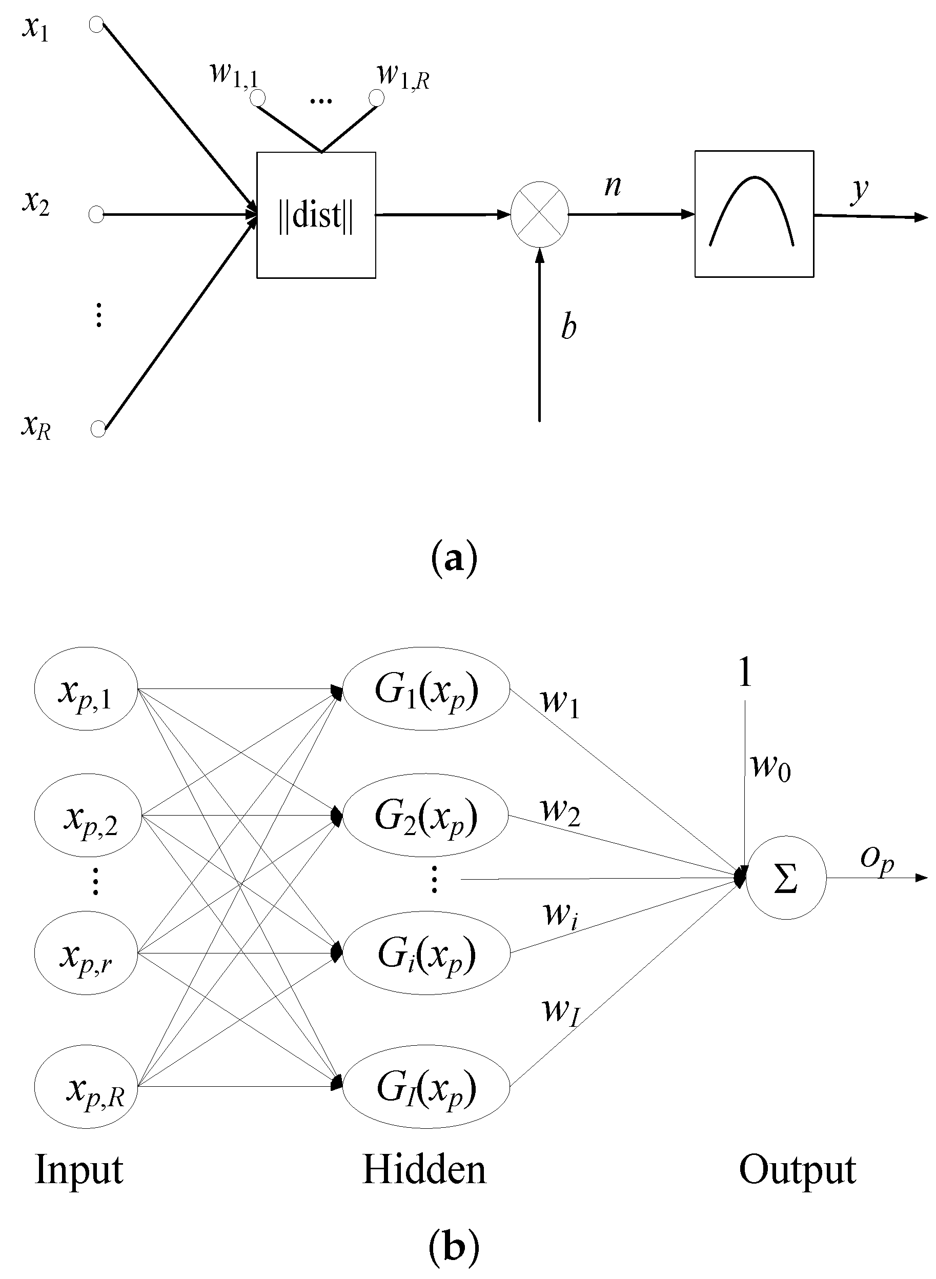
2.2. Artificial Neural Network (ANN) Model

As a class of beneficial non-linear modeling tools, ANN provides advantages when applied to prediction in a number of business areas and is capable of detecting all possible interactions between independent variables [40]. ANN has various network architectures such as multilayer perceptron (MLP) and radial basis function (RBF). In this paper, we test the RBF network for two reasons: first, the main disadvantage of the MLP network is that its local minima are limited and that its astringency is slow [41]; second, the RBF network performs better than the MLP network in terms of approximation capability, classification capacity and learning rate [42]. Broomhead and Lowe [43] initially applied the RBF network, whose neuron model and network structure are illustrated in Figure 1.
The RBF network’s activation function is usually a type of Gaussian radial basis function that can be represented as
G i ( | | x p - c i | | ) = exp { - [ 1 / ( 2 δ i 2 ) ] | | x p - c i | | 2 }
where G i is the i-th Gaussian function, | | x p - c i | | is the Euclidean norm, δ i is the variance of the i-th Gaussian function, x p is the p-th input sample, and c i is the center or average of the i-th Gaussian RBF transformation.
A RBF network is composed of three layers: the input layer contains p input vectors, which have R input signals; the hidden layer is the radial basis layer, which contains I neurons with Gaussian functions; and the output layer is the linearity layer, which is a summing unit of the output weights w I multiplied by the activation function outputs.

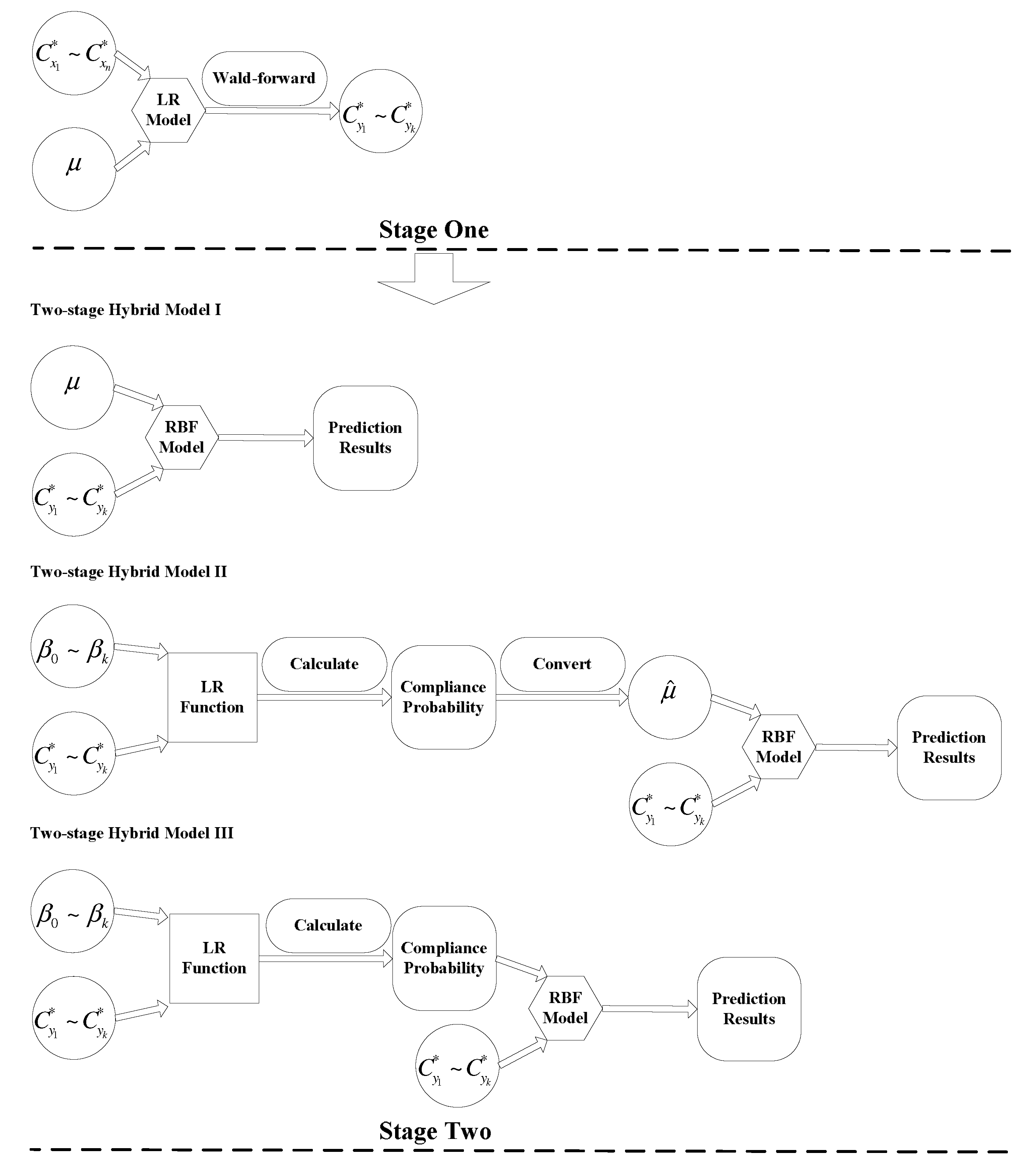
2.3. Two-Stage Hybrid Model

The two-stage hybrid model consists of two stages: in stage one, influencing variables are selected using LR with the Wald-forward method; in stage two, influencing variables are taken as the input variables of the ANN model (i.e., the RBF) [22,26,29]. In this paper, we apply three types of two-stage hybrid models, namely model I, model II and model III. We illustrate these three types of models in Figure 2.

2.3.1. Two-Stage Hybrid Model of LR-ANN I

Model I is constructed using the following procedure: (i) substitute the dependent variable μ and independent variables C x 1 * , C x 2 * , C x 3 * , …, C x n * into the LR model; (ii) use the LR model with the Wald-forward method to identify the independent variables C y 1 * , C y 2 * , C y 3 * , …, C y k * that significantly influence the compliance probability; (iii) the significant variables C y 1 * , C y 2 * , C y 3 * , …, C y k * are used as independent variables and substituted into the input layer of the RBF network model; and the μ is used as the dependent variable of the input layer to obtain a set of prediction values for the compliance probability.

2.3.2. Two-Stage Model of LR-ANN II

Model II is constructed as follows. (i) substitute the dependent variable μ and independent variables C x 1 * , C x 2 * , C x 3 * , …, C x n * into the LR model and (ii) use the LR model with the Wald-forward method to identify the independent variables C y 1 * , C y 2 * , C y 3 * , , C y k * that significantly influence the compliance probability. The function of the LR model can be described as:
p = 1 / [ 1 + e - ( β 0 + β 1 C y 1 * + . . . + β k C y k * ) ]
which is used to obtain the prediction value of the compliance probability for each dataset; (iii) convert the compliance probability into a “negative signal” (value of 0) or “positive signal” (value 1) to produce a new dependent variable μ ^ ; (iv) the significant variables C y 1 * , C y 2 * , C y 3 * , , C y k * are used as the independent variables and substituted into the input layer of the RBF network model; and the new dependent variable μ ^ is used as the dependent variable of the input layer to obtain a set of prediction values for the compliance probability.

2.3.3. Two-Stage Model of LR-ANN III

Model III is constructed using the following steps: (i) substitute the dependent variable μ and independent variables C x 1 * , C x 2 * , C x 3 * , , C x n * into the LR model; (ii) use the LR model with the Wald-forward method to the identify independent variables C y 1 * , C y 2 * , C y 3 * , , C y k * that significantly influence the compliance probability, where the function of the LR model is the same as in Equation (3), which is used to obtain the prediction value of the compliance probability for each dataset; (iii) the significant variables C y 1 * , C y 2 * , C y 3 * , , C y k * are used as the independent variables and substituted into the the input layer of the RBF network model; and finally the prediction value of the compliance probability that is obtained in the anterior process is substituted into the RBF network model as the dependent variable of the input layer to produce a set of prediction values for the compliance probability.

2.4. Methods of Improving the Prediction Accuracy Ratio

To increase the prediction accuracy ratio of the SME credit risk for FIs in SCF, we propose four methods as follows: data normalization, collinearity diagnosis, cross validation and the optimal cutoff point.

2.4.1. Data Normalization Method

The prediction model of SME credit risk involves independent variables that have different units or degrees of variation; therefore, it is necessary to eliminate the effects of variations on the dimension and figures of the independent variables. Bekhet and Eletter [44] emphasized that data normalization can improve the network training capability such as by increasing the data handling efficiency and astringency speed. The normalization method can include a min-max algorithm, a Z-core algorithm, etc. In this paper, we apply the Z-core normalization algorithm which can be described as
C i * = ( C i - C ¯ ) / S i
where C i * are the normalized data, C i are the source data, C ¯ and S i are the average value and the standard deviation of the source data, respectively.

2.4.2. Collinearity Diagnosis Method

We utilize the linear regression method to examine the phenomenon of collinearity and to exclude the variables of collinearity according to Way [45] and Goldstein [46] based on three indices: conditional index (CI), tolerance (T) and variance inflation (VIF). Because the variables with index values of C I > 10 , T < 0 . 2 and V I F > 10 exhibit strong collinearity, we discard the variables whose index values reach the threshold.

2.4.3. Cross Validation Method

Zhang et al. [25], Lin [29], Stone [47] and Efron and Tibshirani [48] prove that the cross-validation method can be used to test and strength the predictive power of models. In this paper, we randomly divide the samples into five groups. When we test the data of one of the five groups, the data of the other four groups are used as training data for the purpose of constructing the model. We obtain the prediction accuracies of the five groups using this method. The final prediction accuracy ratio of the model is measured by the average of the five groups’ test results.

2.4.4. Optimal Cutoff Point Method

To determine the cutoff point for credit risk and improve the prediction accuracy ratio of models, we adopt the optimal cutoff point approach proposed by Hosmer et al. [38], which is calculated based on the point of intersection of sensitivity and specificity according to Hosmer et al. [38] and Lin [29] (see Equation (7)). The sensitivity and specificity is calculated using Equations (8) and (9).
o p t i m a l c u t o f f p o i n t = { [ 1 - m e d i a n ( s e n s i t i v i t y ) ] 2 + [ m e d i a n ( 1 - s p e c i f i c i t y ) ] 2 } 1 / 2
s e n s i t i v i t y = n u m b e r   o f   t r u e   p o s i t i v e s n u m b e r   o f   t r u e   p o s i t i v e s   +   n u m b e r   o f   f a l s e   n e g a t i v e s
s p e c i f i c i t y = n u m b e r   o f   t r u e   n e g a t i v e s n u m b e r   o f   t r u e   n e g a t i v e s   +   n u m b e r   o f   f a l s e   p o s i t i v e s
where “sensitivity” measures the proportion of “actual positives” and is complementary to the “false negative” ratio, “specificity” measures the proportion of “negatives” and is complementary to the “false positive” ratio, and “median” is the median value.

3. Description of Data and Sampling Procedure

3.1. Assumption of Applying Supply Chain Financing (SCF)

SCF has been promoted for almost ten years in China; however, only a few SMEs, CEs and FIs cooperate to facilitate SCF in practice. Thus, we failed to gather enough empirical data in SCF from the references, interviews and surveys. Alternatively, we can use the quarterly financial and non-financial data of selected listed SMEs and CEs on a quarter-by-quarter basis because these SMEs and CEs have real trading relationships with each other. In our study, we assume that these SMEs cooperate with CEs and FIs in SCF, when SMEs are short of capital and starved for financing.

3.2. Variable Definitions

3.2.1. Dependent Variable

The dependent variable represents whether each quarterly data sample of an SME presents a high credit risk signal: a value of 0 indicates a “negative signal”, which means that the SME’s credit risk is high; while a value of 1 indicates a “positive signal”, which means the SME’s credit risk is low. Following Zhu et al. [49], we categorize SMEs into the high and low credit risk groups, depending on whether the SME is a star special treatment (*ST) listed company. The *ST listed SME is the listed company from the Small and Medium Enterprise Board of Shenzhen Stock Exchange that is facing a delisting warning because it has suffered operating losses for two consecutive years. In other words, each quarterly data sample of *ST SMEs presents a “negative signal” in the two years before they are labeled *ST; in contrast, each quarterly data sample of non-*ST SMEs presents a “positive signal” in the past two years.

3.2.2. Independent Variables

In SCF, FIs evaluate the SME credit risks following four factors, which contain some sub-factors: applicant (SME) factor (sub-factors: capability of repayment, operational capability, profitability, development capability and credit rating), counter party (CE) factor (sub-factors: credit rating, capability of repayment and operational capability), items’ characteristic factors (sub-factors: characteristics of trade goods and characteristics of accounts receivable), and operation condition factors (sub-factors: industry status, degree of cooperation and credit worthiness of the applicant). These sub-factors are divided into 18 evaluation indices again according to the suggestions of Xiong et al. [33] and Zhu et al. [49]. These 18 evaluation indices serve as the source independent variables of the LR and ANN models. To facilitate the observation, we describe and define these independent variables as in Table 1.
It is noteworthy that the independent variables shown in Table 1 are financial indicators, except for C 9 , C 13 , C 16 , C 17 and C 18 . Specifically, we obtain the data samples of those 13 financial indexes from the database and collect the data of the remaining five non-financial indexes using the expert evaluation method. The non-financial indexes C 9 , C 13 , C 16 , C 17 and C 18 are considered because they exhibit significant superiority in constructing an SCF SME credit risk evaluation index system compared with traditional SME credit risk evaluation index systems [32,33,34,35]. Therefore, as in References [32,33,34,35], the 18 independent variables fall into five categories: leverage, liquidity, profitability, activity and non-financial.

3.3. Sampling Procedure

In the empirical analysis, the samples are constituted by two sets of data. The first one is the quarterly financial and non-financial data of 77 listed SMEs, which is from the Small and Medium Enterprise Board of Shenzhen Stock Exchange from 31 March 2012 to 31 December 2013. The second one is the quarterly financial and non-financial data of 11 listed CEs which is from the Shanghai Stock Exchange and the Shenzhen Stock Exchange from the period of 31 March 2012 to 31 December 2013, respectively. In our study, 600 valid quarterly data points contained in our data set are used to test the five SME credit risk prediction models. The 11 CEs have a high degree of credit rating, while the 77 listed SMEs include 12 *ST listed companies and 65 non-*ST listed companies.

4. Experimental Results and Analysis

4.1. Experimental Results of Data Normalization

To calculate the results of the normalized data, we apply the Z-core normalization algorithm in Equation (6). In this equation, we first need to estimate the average value and standard deviation of the source data (See Table 2).

4.2. Experimental Results of Collinearity Diagnosis

Because independent variables with values of C I > 10 , T < 0 . 2 and V I F > 10 indicate strong collinearity, we discard variables whose values reach the threshold. The linear regression method is used for diagnosing every independent variable’s threshold values of CI, T and VIF and obtaining 10 independent variables. We present the collinearity diagnosis index values of 18 independent variables and 10 reserved independent variables’ new collinearity diagnosis index values in Table 3. The results of the Analysis of Variance (ANOVA) testing reveal a collinearity with significance reaching the 1% level, as shown in Table 4.

4.3. Experimental Results of Cross Validation

We randomly divide the 600 sample points into five groups with similar sizes and distributions: groups 1, 2, 3, 4 and 5. We choose four of the groups as the training set and the remaining group as the test set. We repeat this process five times to make sure that each group has been tested.

4.4. Experimental Results of Logistic Regression (LR) Model

We use the Wald-forward method of LR for selecting significant independent variables and constructing SME credit risk prediction model. In this paper, the independent variables are excluded from the model when their significance values are larger than 0.01. The empirical LR results show that the independent variables C 6 * , C 9 * , C 12 * and C 14 * persist in the LR model (see Table 5).
Following Table 5, we first represent the LR equation as
ln [ p / ( 1 - p ) ] = - 0 . 282 - 0 . 414 C 6 * + 0 . 866 C 9 * - 0 . 354 C 12 * - 0 . 753 C 14 *
which indicates that the independent variables C 6 * , C 9 * , C 12 * and C 14 * have a significant influence on predicting the credit risk signals of SMEs. Furthermore, because the absolute values of the coefficients of the independent variables C 9 * and C 14 * are substantially larger than those of the other two independent variables, we consider that they have a more prominent influence on predicting the credit risk signals of SMEs. The independent variable C 9 * presents a positive sign, meaning a large “Coefficient” of C 9 * , a high credit rating of CEs and a low credit risk for FIs. In contrast, the independent variable C 14 * presents a negative sign, meaning a large “Coefficient” of C 14 * carries a high credit risk for FIs.
Then, we employ the “Hosmer–Lemeshow test” for assessing the “Goodness of Fit” of the LR model. Following Hosmer et al. [38], in the LR model, we set the significance level to 5% and calculate the degree of freedom (DF) value using the Hosmer–Lemeshow function of SPSS (IBM Company, Chicago, USA). Based on the significance level and the DF, we calculate the critical value of the LR model as 15.507 via the “CHINV” statistics method (see Table 6). For each group testing shown in Table 6, the p-value is greater than 0.05, and the value of the Pearson chi-square is smaller than 15.507, suggesting that the LR model has a good fitting ability.
Finally, we present the optimal cutoff point for the prediction accuracy ratio of the LR model in Table 7. The experimental results show that the mean value of the “positive signal” prediction accuracy ratio is 72.8%, whereas the mean value of the “negative signal” prediction accuracy ratio is only 47.9%.
The above model assumes that the regression coefficients are constant. Other models are also applicable. Examples include the functional-coefficient models, which assume that the coefficients are functions of a state variable [35]. This will be investigated in an ongoing project.

4.5. Experimental Results of the Artificial Neural Network (ANN) Model

In this paper, an RBF network architecture is applied to the ANN model. Therefore, we take 10 independent variables following collinearity diagnosis and use them as the input layer variables of the RBF network model. The single hidden layer of this RBF network includes 20 hidden layer neurons according to the suggestion of Wong [36]. The setting of the mean square error is 0, and the spread value is 1 in our RBF network model.
Table 8 shows that the mean value of the “positive signal” prediction accuracy ratio decreases from 72.8% of the previous model to 70.8%. However, the mean value of the “negative signal” prediction accuracy ratio is obviously increased. Moreover, the overall prediction accuracy ratio also increases from the 61.3% of the LR model to 68.8%.

4.6. Experimental Results of Two-Stage Hybrid Model I

Table 9 shows the experimental results of the two-stage hybrid model I. The mean value of the “positive signal” prediction accuracy ratio reaches 74.9%. Moreover, the overall prediction accuracy ratio also increases from 68.8% of the ANN model to 70.2%. However, the mean of the “negative signal” prediction accuracy ratio falls behind that of the ANN model.

4.7. Experimental Results of Two-Stage Hybrid Model II

Table 10 shows the experimental results of the two-stage hybrid model II. The mean value of the “positive signal” prediction accuracy ratio and the “negative signal” prediction accuracy ratio are both dramatically enhanced. As a result, the overall prediction accuracy ratio reaches 88.5%.

4.8. Experimental Results of Two-Stage Hybrid Model III

Table 11 presents the experimental results of the two-stage hybrid model III. The results show that the mean value of the “positive signal” prediction accuracy ratio decreases from 90.8% for the two-stage hybrid model II to 86.0%. However, the mean value of the “negative signal” prediction accuracy ratio increases from 83.7% for the previous model to 88.6%. As a result, the overall prediction accuracy ratio slightly decreases from 88.5% for the two-stage hybrid model II to 87.4%. According to Bekhet and Eletter [44], Yap et al. [52], Kürüm et al. [53] and West [54], we consider that the improvement of the “negative signal” prediction accuracy ratio is more important than that of the “positive signal” prediction accuracy ratio; therefore, the two-stage hybrid model III exhibits a better credit risk prediction capability than model II.

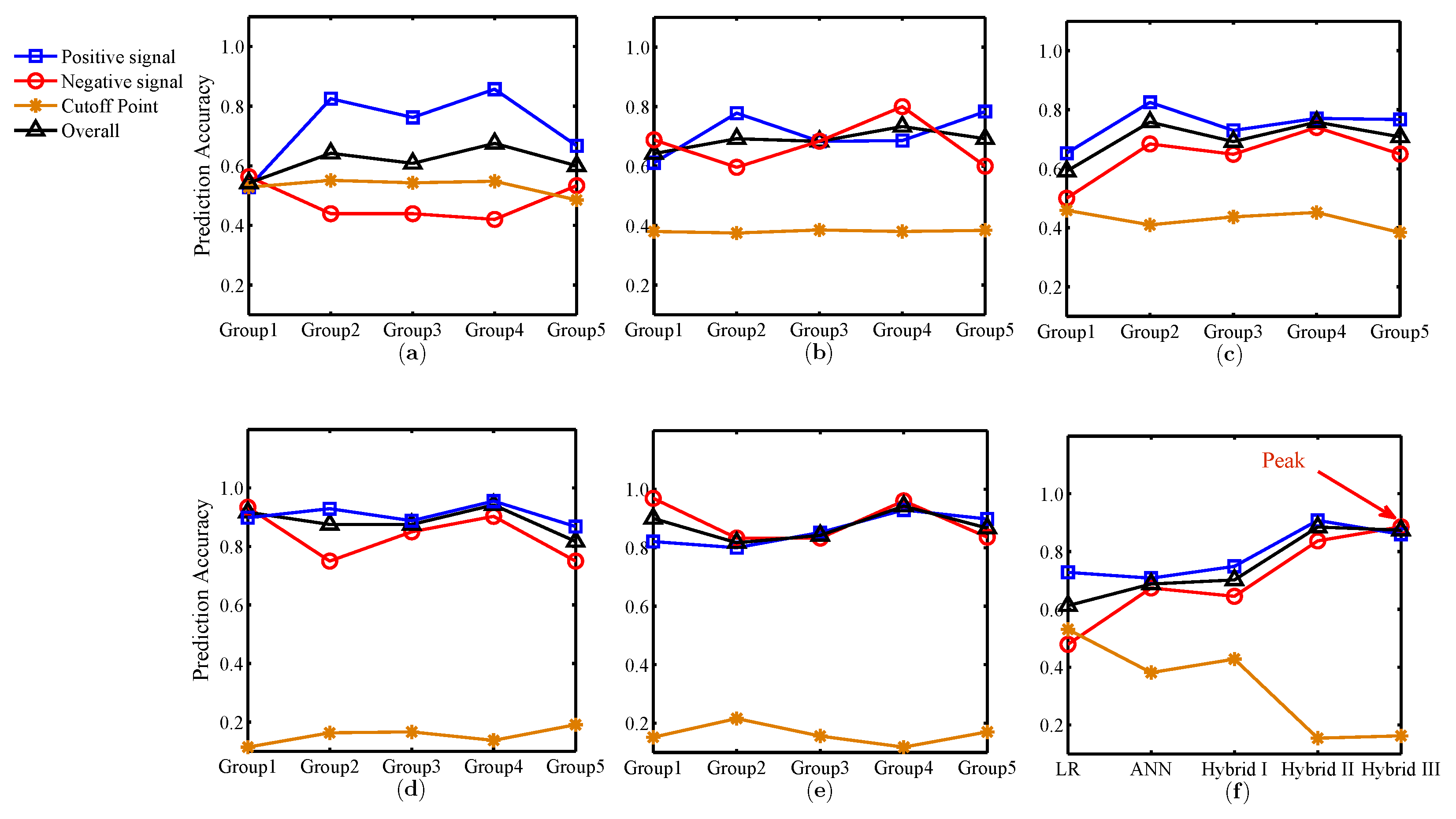
4.9. Comparing the SME Credit Risk Prediction Accuracies of the Five Models

Hosmer et al. [38] argued that a better and more complete description of classification accuracy is the area under the Receiver Operating Characteristic (ROC) curve and provided general guidelines as follows:
(1)
If ROC = 0.5, it means no discrimination.
(2)
If 0.5 < ROC < 0.7, it means poor discrimination.
(3)
If 0.7 < ROC < 0.8, it means acceptable discrimination.
(4)
If 0.8 < ROC < 0.9, it means excellent discrimination.
(5)
If ROC ≥0.9, it means outstanding discrimination.
Thus, we present these five models’ areas under the ROC curve in Table 12.
Table 12 shows that the two-stage hybrid models II and III demonstrate outstanding performance in terms of discrimination. To compare the SME credit risk prediction accuracy ratios of the five models in detail, we illustrate the credit prediction accuracy ratios of the LR model, the ANN model and the three types of two-stage hybrid models of LR-ANN in Figure 3, where the red marks indicate the “negative signal” prediction accuracy ratios, the blue marks indicate the “positive signal” prediction accuracy ratios, the black marks indicate the overall signal prediction accuracy ratios, and the orange marks indicate the optimal cutoff point for predictive values. Panels (a–e) depict the five groups’ test results of the SME credit risk prediction accuracy ratios under the five prediction models. Panel (f) illustrates that, from the first model to the fifth model, the average prediction accuracy ratios follow a stepwise uptrend. Meanwhile, we can find that the average “negative signal” prediction accuracy ratio of the two-stage hybrid model III reaches a peak in panel (f). Specifically, the two-stage hybrid model III is better than the other four models in terms of finding the bad applications. Thus, we propose that China’s FIs should apply the two-stage hybrid model III to predict the SME credit risk in SCF.

5. Conclusions

In this paper, we investigated the quarterly financial and non-financial data of 77 listed SMEs and 11 listed core enterprises CEs in China during the period of 2012–2013. Specifically, we constructed a new SME credit risk evaluation index system and five types of SME credit risk prediction models for China’s FIs in SCF. We first normalized the source data, excluded independent variables with strong collinearity, and randomly divided the samples into five groups for the purpose of model testing and construction. Then, we built five credit prediction models using the LR approach, the ANN approach and a hybrid approach.
Some basic findings for predicting SME credit risk in this study can be summarized as follows: (i) evaluating the credit risks of SMEs in SCF from four aspects, including applicants (SMEs), counter parties (CEs), items’ characteristics and operation situation; (ii) the variables C 6 * , C 9 * , C 12 * and C 14 * significantly influence the SME credit risk signals prediction accuracy ratio; and (iii) the two-stage hybrid model III is better than the other four models in predicting “negative signals”. Because we consider that improving the ratio of bad applicant prediction accuracy is more important than improving the ratio of good applicant prediction accuracy for FIs at the present stage of China’s credit market, we affirm that the two-stage hybrid model III provides a better SME credit risk signal prediction capability than other models do.
In practice, the two-stage hybrid model III can also be used to predict other SMEs’ credit risk signals in SCF. For instance, there are eight quarterly data samples of other SMEs and CEs for two consecutive years that are not included in existing datasets; we filter out the data on the profit margin on sales of SMEs ( C 6 * ), the credit rating of ( C 9 * ), profit margin on sales of CEs ( C 12 * ) and accounts receivable collection period of SMEs ( C 14 * ) from data samples as the input layer of the two-stage hybrid model III. Then, we obtain a value of 0 or 1 from the output layer when we run the model. We define a value of 0 as a “negative signal” and a value of 1 as a “positive signal”. If we obtain eight 0 s, this indicates an extremely high credit risk, whereas if we obtain eight 1s, this indicates a relatively low credit risk; thus, the credit risk level of an SME depends on how many 0 s or 1s we obtain. In other words, the more 0 s we obtain, the more credit issues the SME has and vice versa. Unfortunately, only a few of China’s SMEs and CEs have cooperated on SCF over the past decade. Therefore, we have been unable to obtain adequate cases and data samples concerning SCF in practice. In future research, it will be worthwhile to find Chinese SMEs and CEs that not only have real trading relationships but also implement SCF together. This will allow China’s financial institutions to make better financing decisions in SCF.

Acknowledgments

This work was supported by the National Natural Science Foundation of China under Grant No. 71373072 and No. 71501066; the China Scholarship Council under Grant No. 201506135022; the Specialized Research Fund for the Doctoral Program of Higher Education under Grant No. 20130161110031; and the Foundation for Innovative Research Groups of the National Natural Science Foundation of China under Grant No. 71521061.

Author Contributions

All authors discussed and agreed on the ideas and scientific contributions. You Zhu and Chi Xie performed the simulations and wrote the simulation sections. You Zhu, Chi Xie, Gang-Jin Wang and Xin-Guo Yan did the mathematical modeling in the manuscript. Chi Xie, Bo Sun and Gang-Jin Wang contributed to manuscript writing and revisions.

Conflicts of Interest

The authors declare no conflict of interest.

References

  1. Hofmann, E. Von der strategie bis zur finanziellen steuerung der performance in supply chains. In Interorganizational Operations Management; Springer Fachmedien Wiesbaden: Wiesbaden, Germany, 2013; pp. 1–20. [Google Scholar]
  2. More, D.; Basu, P. Challenges of supply chain finance: A detailed study and a hierarchical model based on the experiences of an Indian firm. Bus. Process Manag. J. 2013, 19, 624–647. [Google Scholar] [CrossRef]
  3. Knox, A. Electronic payment: The missing link in supply chain efficiency. J. Financ. Transform. Mark. Imperfect. 2005, 14, 16–18. [Google Scholar]
  4. Fairchild, A. Intelligent matching: Integrating efficiencies in the financial supply chain. Supply Chain Manag. 2005, 10, 244–248. [Google Scholar] [CrossRef]
  5. Hofmann, E.; Belin, O. Value proposition of SCF. In Supply Chain Finance Solutions: Relevancel—Propositions— Market Value; Springer: Berlin, Germany; 2011; pp. 41–45. [Google Scholar]
  6. Gomm, M.L. Supply chain finance: Applying finance theory to supply chain management to enhance finance in supply chains. Int. J. Logist. Res. Appl. 2010, 13, 133–142. [Google Scholar] [CrossRef]
  7. Sopranzetti, B.J. Selling accounts receivable and the underinvestment problem. Q. Rev. Econ. Financ. 1999, 39, 291–301. [Google Scholar] [CrossRef]
  8. Seifert, R.W.; Seifert, D. Financing the chain. Int. Commer. Rev. 2011, 10, 32–44. [Google Scholar] [CrossRef]
  9. Wuttke, D.A.; Blome, C.; Henke, M. Focusing the financial flow of supply chains: An empirical investigation of financial supply chain management. Int. J. Prod. Econ. 2013, 145, 773–789. [Google Scholar] [CrossRef]
  10. Gouvêa, M.A.; Gonçalves, E.B. Credit risk analysis applying logistic regression, neural networks and genetic algorithms models. In Proccedings of the POMS 18th Annual Conference, Dallas, TX, USA, 4–7 May 2007; 2007; pp. 4–7. [Google Scholar]
  11. Lahsasna, A.; Ainon, R.N.; Teh, Y.W. Credit scoring models using soft computing methods: A survey. Int. Arab J. Inf. Technol. 2010, 7, 115–123. [Google Scholar]
  12. Wu, C.; Guo, Y.; Zhang, X.; Xia, H. Study of personal credit risk assessment based on support vector machine ensemble. Int. J. Innov. Comput. Inf. Control. 2010, 6, 2353–2360. [Google Scholar]
  13. Burgt, M.J.V.D. Calibrating low-default portfolios, using the cumulative accuracy profile. J. Risk Model Valid. 2007, 1, 1–17. [Google Scholar]
  14. Harrell, F.E.; Lee, K.L. A comparison of the discrimination of discriminant analysis and logistic regression under multivariate normality. In Biostatistics: Statistics in Biomedical, Public Health and Environmental Sciences; North-Holland: New York, NY, USA, 1985; pp. 333–343. [Google Scholar]
  15. Altman, E.I.; Sabato, G. Effects of the New Basel Capital Accord on bank capital requirements for SMEs. J. Financ. Serv. Res. 2005, 28, 15–42. [Google Scholar] [CrossRef]
  16. Altman, E.I.; Sabato, G. Modelling credit risk for SMEs: Evidence from the US market. Abacus J. Acc. Financ. Bus. Stud. 2007, 43, 332–357. [Google Scholar] [CrossRef]
  17. Behr, P.; Güttler, A. Credit risk assessment and relationship lending: An empirical analysis of German small and medium-sized enterprises. J. Small Bus. Manag. 2007, 45, 194–213. [Google Scholar] [CrossRef]
  18. Fantazzini, D.; Figini, S. Default forecasting for small-medium enterprises: Does heterogeneity matter. Int. J. Risk Assess. Manag. 2009, 11, 38–49. [Google Scholar] [CrossRef]
  19. Fidrmuc, J.; Heinz, C. Default rates in the loan market for SMEs: Evidence from Slovakia. Econ. Syst. 2009, 34, 133–147. [Google Scholar] [CrossRef]
  20. Pederzoli, C.; Torricelli, C. A parsimonious default prediction model for Italian SMEs. Banks Bank Syst. 2010, 5, 28–32. [Google Scholar]
  21. Pederzoli, C.; Thoma, G.C. Modelling credit risk for innovative firms: The role of innovation measures. J. Financ. Serv. Res. 2013, 44, 111–129. [Google Scholar] [CrossRef]
  22. Lee, T.S.; Chen, I.F. A two-stage hybrid credit scoring model using artificial neural networks and multivariate adaptive regression splines. Expert Syst. Appl. 2005, 28, 743–752. [Google Scholar] [CrossRef]
  23. Salchenberger, L.M.; Cinar, E.M.; Lash, N.A. Neural networks: A new tool for predicting thrift failures. Decis. Sci. 1992, 23, 899–916. [Google Scholar] [CrossRef]
  24. Sharda, R.; Wilson, R.L. Neural Network experiments in business-failure forecasting: Predictive performance measurement issues. Int. J. Comput. Intell. Organ. 1996, 1, 107–117. [Google Scholar]
  25. Zhang, G.; Hu, M.Y.; Patuwo, B. Artificial neural networks in bankruptcy prediction: General framework and cross-validation analysis. Eur. J. Oper. Res. 1999, 166, 16–32. [Google Scholar] [CrossRef]
  26. Lee, T.S.; Chiu, C.C.; Lu, C.J.; Chen, I.F. Credit scoring using the hybrid neural discriminant technique. Expert Syst. Appl. 2002, 23, 245–254. [Google Scholar] [CrossRef]
  27. Chung, H.M.; Gray, P. Special section: Data mining. J. Manag. Inf. Syst. 1999, 16, 11–16. [Google Scholar] [CrossRef]
  28. Craven, M.W.; Shavlik, J.W. Using neural networks for data mining. Future Gener. Comput. Syst. 1997, 13, 211–229. [Google Scholar] [CrossRef]
  29. Lin, S.L. A new two-stage hybrid approach of credit risk in banking industry. Expert Syst. Appl. 2009, 36, 8333–8341. [Google Scholar] [CrossRef]
  30. Falavigna, G. Models for Default Risk Analysis: Focus on Artificial Neural Networks, Model Comparisons, Hybrid Frameworks. Available online: http://www.ceris.cnr.it/ceris/workingpaper/2006/WP_10_06_FALAVIGNA.pdf (accessed on 28 April 2016).
  31. Deng, A.M.; Xiong, J.; Zhang, F. Order financing risk pre-warning model based on BP network. J. Intell. 2010, 29, 23–28. [Google Scholar]
  32. Bai, S.Z.; Li, S. Supply chain finance risk evaluation research based on BP neural network. Commer. Res. 2013, 6, 27–31. [Google Scholar]
  33. Xiong, X.; Ma, J.; Zhao, W. Credit risk analysis of supply chain finance. Nankai Bus. Rev. 2009, 12, 92–98. [Google Scholar]
  34. Bai, S.B. A research into the risk early-warning of enterprise supply chain financing based on ordered logistic model. Econ. Surv. 2010, 6, 66–71. [Google Scholar]
  35. Bei, Y.H.; Yang, L.; Wang, Y.H. Credit risk evaluation of car-making industry under supply chain financing mode. Logist. Technol. 2012, 31, 379–382. [Google Scholar]
  36. Jiang, J.; Jiang, X.; Song, X. Weighted composite quantile regression estimation of DTARCH models. Econ. J. 2014, 17, 1–23. [Google Scholar] [CrossRef]
  37. Jiang, X.; Song, X.; Xiong, Z. Efficient and robust estimation of GARCH models. J. Test. Eval. 2015. [Google Scholar] [CrossRef]
  38. Hosmer, J.D.W.; Lemeshow, S.; Sturdivant, R.X. Area under the receiver operating characteristic curve. In Applied Logistic Regression; John Wiley & Sons: Hoboken, NJ, USA, 2013; pp. 184–197. [Google Scholar]
  39. Fidell, L.S.; Tabachnick, B.G. Fundmental equations for multiple regression. In Using Multivariate Statistics; Harper Collins: Boston, MA, USA, 2008; pp. 128–134. [Google Scholar]
  40. Li, J.; Burke, E.K.; Qu, R. Integrating neural networks and logistic regression to underpin hyper-heuristic search. Knowl. Based Syst. 2011, 24, 322–330. [Google Scholar] [CrossRef]
  41. Masters, T. Probabilistic neural networks I: Introduction. In Advanced Algorithms for Neural Networks: A C++ Sourcebook; John Wiley & Sons: New York, NY, USA, 1995; pp. 112–120. [Google Scholar]
  42. Gutierrez, P.A.; Segovia-Vargas, M.J.; Salcedo-Sanz, S.; Hervas-Martinez, C.; Sanchis, A.; Portilla-Figueras, J.A.; Fernandez-Navarro, F. Hybridizing logistic regression with product unit and RBF networks for accurate detection and prediction of banking crises. Omega 2010, 38, 333–344. [Google Scholar] [CrossRef]
  43. Broomhead, D.S.; Lowe, D. Radial basis functions, multi-variable functional interpolation and adaptive networks. DTIC Doc. 1988, 2, 321–355. [Google Scholar]
  44. Bekhet, H.A.; Eletter, S.F.K. Credit risk assessment model for Jordanian commercial banks: Neural scoring approach. Rev. Dev. Financ. 2014, 4, 20–28. [Google Scholar] [CrossRef]
  45. Way, Y. Collinearity diagnosis for a relative risk regression analysis an application to assessment of diet cancer relationship in epidemiological studies. Stat. Med. 1992, 11, 1273–1287. [Google Scholar]
  46. Goldstein, R. Book reviews: Conditioning diagnostics: Collinearity and weak data in regression. Technometrics 1993, 35, 85–86. [Google Scholar] [CrossRef]
  47. Stone, M. Cross-validatory choice and assessment of statistical predictions. J. R. Stat. Soc. 1974, 36, 111–147. [Google Scholar]
  48. Efron, B.; Tibshirani, R.J. Crossvalidation and other estimates of prediction. In An Introduction to the Bootstrap; Chapman and Hall: New York, NY, USA, 1993; pp. 237–257. [Google Scholar]
  49. Zhu, Y.; Xie, C.; Wang, G.; Yan, X. Comparison of individual, ensemble and integrated ensemble machine learning methods to predict China’s SMEs credit risk in supply chain finance. Neural Comput. Appl. 2016. [Google Scholar] [CrossRef]
  50. Jiang, J. Multivariate Functional-coefficient regression models for multivariate nonlinear times series. Biometrika 2014, 101, 689–702. [Google Scholar] [CrossRef]
  51. Wong, F.S. Time series forecasting using backpropagation neural networks. Neurocomputing 1991, 2, 147–159. [Google Scholar] [CrossRef]
  52. Yap, B.W.; Ong, S.H.; Husain, N.H.M. Using data mining to improve assessment of credit worthiness via credit scoring models. Expert Syst. Appl. 2011, 38, 13274–13283. [Google Scholar] [CrossRef]
  53. Kürüm, E.; Yildirak, K.; Weber, G.W. A classification problem of credit risk rating investigated and solved by optimization of ROC curve. Cent. Eur. J. Oper. Res. 2012, 20, 529–557. [Google Scholar] [CrossRef]
  54. West, D. Neural network credit scoring models. Comput. Oper. Res. 2000, 27, 1131–1152. [Google Scholar] [CrossRef]
Figure 1. A neuron model of radial basis function (RBF) network is considered and includes a neuron with R input signals, the R input signals with w connection weights, the Euclidean distance between input vectors and weight vectors with | | d i s t | | , the threshold value as b, the independent variable of the activation function as n and the activation function as y. The structure of a three-layer radial basis neural network is considered and includes an input layer with x p input variables, a single hidden layer with G I Gaussian radial basis functions, output weights as w I and an output layer with one neuron. (a) a neuron model of radial basis function network; (b) the structure of a three-layer radial basis neural network.
Sustainability 08 00433 g001
Figure 2. The two-stage hybrid models of LR-ANN (integrated by logistic regression and artificial neural network) are illustrated. In stage one, the independent variables C x 1 * C x n * and the dependent variable μ are substituted into the LR model using the Wald-forward method to indentify the independent variables C y 1 * C y k * that significantly influence the compliance probability. In stage two, the two-stage hybrid model I is established using μ and C y 1 * C y k * ; the two-stage hybrid model II is established using μ ^ and C y 1 * C y k * ; the two-stage hybrid model III is established using the prediction value of compliance probability and C y 1 * C y k * ; the prediction value of compliance probability for each data sample is calculated by LR function; and the new dependent variable μ ^ is obtained by converting the compliance probability into a“negative signa” (value of 0) or a “ositive signa” (value of 1).
Sustainability 08 00433 g002
Figure 3. Comparing the SME credit risk signal prediction accuracy ratios of five models, this shows that the average “negative signal” prediction accuracy ratio of the two-stage hybrid model III reaches a peak. (a) Prediction accuracy ratios of the logistic regression; (b) prediction accuracy ratios of the artificial neural network; (c) prediction accuracy ratios of the two-stage hybrid model I; (d) prediction accuracy ratios of the two-stage hybrid model II; (e) prediction accuracy ratios of the two-stage hybrid model III; (f) mean prediction accuracy ratios of five models;
Sustainability 08 00433 g003
Table 1. List of independent variables [49].
IndexesVariablesCategories
C 1 Current ratio of SMELiquidity
C 2 Quick ratio of SMELiquidity
C 3 Cash ratio of SMELiquidity
C 4 Working capital turnover of SMELiquidity
C 5 Return on equity of SMELeverage
C 6 Profit margin on sales of SMEProfitability
C 7 Rate of Return on Total Assets of SMELeverage
C 8 Total Assets Growth Rate of SMEActivity
C 9 Credit rating of CENon-financial
C 10 Quick ratio of CELiquidity
C 11 Turnover of total capital of CELiquidity
C 12 Profit margin on sales of CEProfitability
C 13 Price rigidity, liquidation and vulnerable degree of trade goodsNon-financial
C 14 Accounts receivable collection period of SMELeverage
C 15 Accounts receivable turnover ratio of SMELeverage
C 16 Industry trends of SMENon-financial
C 17 Transaction time and transaction frequency of SMENon-financial
C 18 Credit rating of SMENon-financial
Note on Abbreviations: SME: medium-sized enterprise; CE: core enterprise.
Table 2. Descriptive statistics of the mean and standard deviation of 600 samples.
Independent VariablesObservationsMeanStd. Deviation
C 1 6001.7941.665
C 2 6001.3511.539
C 3 6000.5740.916
C 4 60014.56671.026
C 5 6000.0490.074
C 6 6000.0510.080
C 7 6000.0280.037
C 8 6000.2210.258
C 9 6008.1552.702
C 10 6000.9900.204
C 11 6000.8360.451
C 12 6000.04190.027
C 13 6006.3002.278
C 14 60076.70949.361
C 15 6006.7519.670
C 16 6005.6952.012
C 17 6006.3002.278
C 18 6005.6952.012
Table 3. Collinearity diagnosis index value.
Independent VariablesOriginal 18 VariablesReserved 10 Variables d
T a VIF b CI c TVIFCI
C 1 * 0.008126.1751.195
C 2 * 0.006169.7471.230
C 3 * 0.08411.9751.584
C 4 * 0.9111.0981.7920.9331.0721.173
C 5 * 0.1218.2361.909
C 6 * 0.3562.8071.9340.7371.3581.455
C 7 * 0.1089.2362.088
C 8 * 0.6971.4342.1700.8231.2151.503
C 9 * 0.3922.5522.6440.5181.9321.549
C 10 * 0.5331.8763.0620.6361.5731.573
C 11 * 0.6921.4463.5910.7141.4001.701
C 12 * 0.4452.2003.8270.5221.9151.985
C 13 *
C 14 * 0.5021.9914.1370.5571.7962.539
C 15 * 0.4372.2896.9950.4582.1842.767
C 16 *
C 17 * 0.4772.0947.8740.5341.8743.211
C 18 * 0.4712.12433.233
a T denotes “Tolerance”; b VIF denotes “Variance Inflation”; c CI denotes “Conditional Index”; d There are 10 independent variables that are reserved by the collinearity diagnosis, and these reserved independent variables are used for structuring the credit risk prediction model.
Table 4. Collinearity diagnosis index value.
ModelSum of SquaresdfMean SquareFSig a
Regression35.023162.18911.2270.000
Residual Total113.6705830.195
148.693599
a Significance at 1% level.
Table 5. Significance values of independent variables.
Independent VariablesB. a Sig. b Situation c
C 4 * 0.1690.681Excluded
C 6 * −0.4140.000Reserved
C 8 * 0.2390.017Excluded
C 9 * 0.8660.000Reserved
C 10 * 0.2810.015Excluded
C 11 * −0.1760.085Excluded
C 12 * −0.3540.003Reserved
C 14 * −0.7530.000Reserved
C 15 * 0.1230.762Excluded
C 17 * 1.4050.236Excluded
Constant d −0.2820.003Reserved
a B. denotes “Coefficient”; b Sig. denotes “Significance”; c The independent variables are excluded when their significance values are greater than 0.01; d Constant denotes “intercept”.
Table 6. Hosmer–Lemeshow test of an logistic regression model.
Group 1Group 2Group 3Group 4Group 5
Pearson chi-square8.8088.81010.83011.1993.068
Degree of freedom8.0008.0008.0008.0008.000
p-value0.1600.3590.2120.1910.930
Critical value15.50715.50715.50715.50715.507
Table 7. Optimal cutoff point for the prediction accuracy ratio of the logistic regression model.
Group 1Group 2Group 3Group 4Group 5Mean (SD)
Optimal cutoff point a 0.5280.5510.5430.5480.4850.531 (0.027)
Positive signal52.8%82.5%76.2%85.7%66.7%72.8% (0.133)
Negative signal56.3%43.9%43.9%42.0%53.3%47.9% (0.065)
Overall54.2%64.2%60.8%67.5%60.0%61.3% (0.050)
a The optimal cutoff point is determined by taking the point of the intersection of the sensitivity and specificity curves.
Table 8. Optimal cutoff point for the prediction accuracy ratio of the artificial neural network model.
Group 1Group 2Group 3Group 4Group 5Mean (SD)
Optimal cutoff point a 0.3800.3750.3850.3800.3840.381 (0.004)
Positive signal61.1%77.8%68.3%68.6%78.3%70.8% (0.073)
Negative signal68.8%59.6%68.4%80.0%60.0%67.4% (0.083)
Overall64.2%69.2%68.3%73.3%69.2%68.8% (0.032)
a The optimal cutoff point is determined by taking the point of intersection of the sensitivity and specificity curves.
Table 9. Optimal cutoff point for the prediction accuracy ratio of the two-stage hybrid model I.
Group 1Group 2Group 3Group 4Group 5Mean (SD)
Optimal cutoff point a 0.4590.4100.4370.4520.3840.428 (0.031)
Positive signal65.3%82.5%73.0%77.1%76.7%74.9% (0.064)
Negative signal50.0%68.4%64.9%74.0%65.0%64.5% (0.089)
Overall59.2%75.8%69.2%75.8%70.8%70.2% (0.068)
a The optimal cutoff point is determined by taking the point of intersection of the sensitivity and specificity curves.
Table 10. Optimal cutoff point for the prediction accuracy ratio of the two-stage hybrid model II.
Group 1Group 2Group 3Group 4Group 5Mean (SD)
Optimal cutoff point a 0.1140.1630.1660.1370.1910.154 (0.030)
Positive signal89.8%92.9%88.8%95.5%86.8%90.8% (0.035)
Negative signal93.4%75.0%85.0%90.3%75.0%83.7% (0.085)
Overall91.7%87.5%87.5%94.2%81.7%88.5% (0.048)
a The optimal cutoff point is determined by taking the point of intersection of the sensitivity and specificity curves.
Table 11. Optimal cutoff point for the prediction accuracy ratio of the two-stage hybrid model III.
Group 1Group 2Group 3Group 4Group 5Mean (SD)
Optimal cutoff point a 0.1520.2160.1560.1180.1700.162 (0.036)
Positive signal82.1%80.0%85.2%92.9%89.8%86.0% (0.053)
Negative signal96.9%83.3%83.3%96.0%83.6%88.6% (0.072)
Overall90.0%81.7%84.2%94.2%86.7%87.4% (0.049)
a The optimal cutoff point is determined by taking the point of intersection of the sensitivity and specificity curves.
Table 12. Discrimination accuracies of the five models.
ModelsGroup 1Group 2Group 3Group 4Group 5Mean (SD)Discrimination Accuracy a
LR0.6080.6110.6230.6280.6530.625 (0.018)No
ANN0.8110.8350.8090.8120.8250.818 (0.011)Excellent
Hybrid I0.7510.7960.7640.7640.8190.779 (0.028)Acceptable
Hybrid II0.9740.9580.9590.9670.9520.962 (0.009)Outstanding
Hybrid III0.9590.9400.9630.9680.9590.958 (0.011)Outstanding
a The rule of the discrimination accuracy was proposed by Hosmer et al. [38].

