Article

Study on Solar Radiation Models in South Korea for Improving Office Building Energy Performance Analysis

1
Building and Urban Research Institute, Korea Institute of Civil Engineering and Building Technology, 283 Goyangdae-Ro, Ilsanseo-Gu, Goyang-Si, Gyeonggi-Do 10223, Korea
2
Department of Architectural Design, Dongseo University, 47 Jurye-Ro, Sasang-Gu, Busan 47011, Korea
3
Department of Architectural Engineering, Ewha Womans University, 52, Ewhayeodae-Gil, Seodaemun-Gu, Seoul 03760, Korea
*
Author to whom correspondence should be addressed.
Sustainability 2016, 8(6), 589; https://0-doi-org.brum.beds.ac.uk/10.3390/su8060589
Submission received: 16 May 2016 / Revised: 19 June 2016 / Accepted: 20 June 2016 / Published: 22 June 2016
(This article belongs to the Section Sustainable Engineering and Science)

Abstract

:
Hourly global solar radiation in a weather file is one of the significant parameters for improving building energy performance analyses using simulation programs. However, most weather stations worldwide are not equipped with solar radiation sensors because they tend to be difficult to manage. In South Korea, only twenty-two out of ninety-two weather stations are equipped with sensors, and there are large areas not equipped with any sensors. Thus, solar radiation must often be calculated by reliable solar models. Hence, it is important to find a reliable model that can be applied in the wide variety of weather conditions seen in South Korea. In this study, solar radiation in the southeastern part of South Korea was calculated using three solar models: cloud-cover radiation model (CRM), Zhang and Huang model (ZHM), and meteorological radiation model (MRM). These values were then compared to measured solar radiation data. After that, the calculated solar radiation data from the three solar models were used in a building energy simulation for an office building with various window characteristics conditions, in order to identify how solar radiation differences affect building energy performance. It was found that a seasonal solar model for the area should be developed to improve building energy performance analysis.

1. Introduction

To analyze building energy performance using building energy simulation programs, detailed simulation inputs, including building envelope characteristics, mechanical and electrical systems inputs of a targeted building, and appropriate weather files, are all necessary. Appropriate weather files include reliable weather parameter data measured from a location where a targeted building is located; this compilation includes hourly dry-bulb, wet-bulb, and dew-point temperatures; wind direction and speed; atmospheric pressure; and solar radiation. For solar radiation, most simulation programs generally require two of the following: global horizontal, horizontal diffuse, and direct normal solar radiation.
Ninety-two manned weather stations are currently stationed across South Korea, and weather data, which is measured every hour, can be obtained from the Korea Meteorological Administration’s webpage [1]. However, only twenty-two weather stations in major cities, including Seoul, Busan, Daegu, Gwangju, etc., have equipment for measuring solar radiation [2]. Thus, if solar radiation data are required for areas outside of major cities, they must be calculated using reliable solar radiation models.
For similar reasons, since the 1970s a number of global solar radiation models have been developed by various countries in Europe, North America, and Asia; they rely on local climates, and have been regularly improved over time. These models can be divided into three types: regression, mechanistic, and state-of-the-art. Cloud-cover radiation model (CRM) [3] and Zhang and Huang model (ZHM) [4] are representative of regression-type models, while the meteorological radiation model (MRM) [5] and upper-air humidity model [6] are mechanistic, and models that use special devices, such as satellite data [7,8], fall into the final category. Each model has its pros and cons. For instance, a regression-type model can be inconvenient because it requires the calculation of site-specific coefficients derived from a correlation between the past few years of measured solar radiation data and other weather data. However, once the necessary coefficients are calculated, they can easily be applied to other nearby locations with similar climate conditions. A mechanistic-type model does not require the calculation of site-specific coefficients; instead, it needs a significant number of weather parameters in order to calculate the transmittance of solar radiation through the air and to the ground. Moreover, some of these parameters, such as sunshine duration, are not commonly provided by local weather stations. Finally, state-of-the-art-type models that use satellite data can provide comparatively accurate prediction [9], but they require specialized knowledge to extract necessary information from the satellite data. The main concept for calculating solar radiation from the satellite data is similar to other solar models; solar radiation is calculated from the interactions of extraterrestrial radiation with the atmosphere in the Earth, which are reflected and absorbed radiation in the air, and absorbed radiation on the ground. In these interactions, the solar radiation reflected in the air is derived from the satellite radiometer. The following three models can be a representative models using the satellite data: heliosat model [10], operational model [7] and Jajai model [11].
This study uses several solar models that were summarized in a report from the American Society of Heating, Refrigerating, Air-conditioning Engineers (ASHRAE) [12], including CRM, ZHM, and MRM. During the selection process, solar models using monthly or daily weather data were excluded as candidates because hourly weather data is required to run hourly building energy simulation programs. In addition, solar models that require weather parameters not commonly provided by local weather stations (such as sunshine duration or satellite images) were also excluded. Once the three models were selected, they were applied to a major city, Busan, which is located in the southeast corner of South Korea, in order to determine which solar model would be the most appropriate for the area. In addition, the solar models selected in this study were modified to be fitted in the climate in Busan (please see Section 2.1 for details).
Even though several studies have been conducted on improving the accuracy of hourly global solar radiation models, few have addressed how solar radiation data calculated from a solar model affects building energy performance analyses when building energy simulation programs are used. There were two works found in the literature review conducted for this research: Seo and Krarti [13], and Wan et al. [14]. Seo and Krarti calculated global horizontal solar radiation in tropical areas using Zhang and Huang, Kasten, Muneer, and neural network models, and they created weather files to compare office building energy performances using a simulation program. They concluded that the Zhang and Huang Model was the most accurate for tropical areas with a high level of reliability. In a similar fashion, Wan et al. used two parameter regression models to calculate global solar radiation in nine locations in China; they then conducted building energy simulations to determine how building energy consumption differed according to two calculated solar radiation levels. However, both of these studies focused on comparing building energy consumptions according to different solar radiation data. They did not extend their analyses to determine reasons for these differences or how the solar models could be improved for future work in this area.
Therefore, as a preliminary step to developing a new solar model for building energy performance analyses in South Korea, this study predicted solar radiation in the southeast corner of South Korea by calculating and analyzing existing solar models; then, an office building energy performance was evaluated using the calculated solar radiation data.

2. Results

2.1. Global Solar Radiation Models

Generally, solar radiation from an overcast sky is difficult to predict because there are various factors in the air that cause effects like reflection, absorption, and the emittance of solar radiation; these depend on local weather conditions. Therefore, in this study three existing solar models (i.e., CRM, ZHM, and MRM) were applied to calculate solar radiation in the southeast corner of South Korea, specifically the city of Busan, in order to determine the most appropriate solar model for use in this area. The characteristics and calculation process of each solar radiation model are shown in the following subsections.

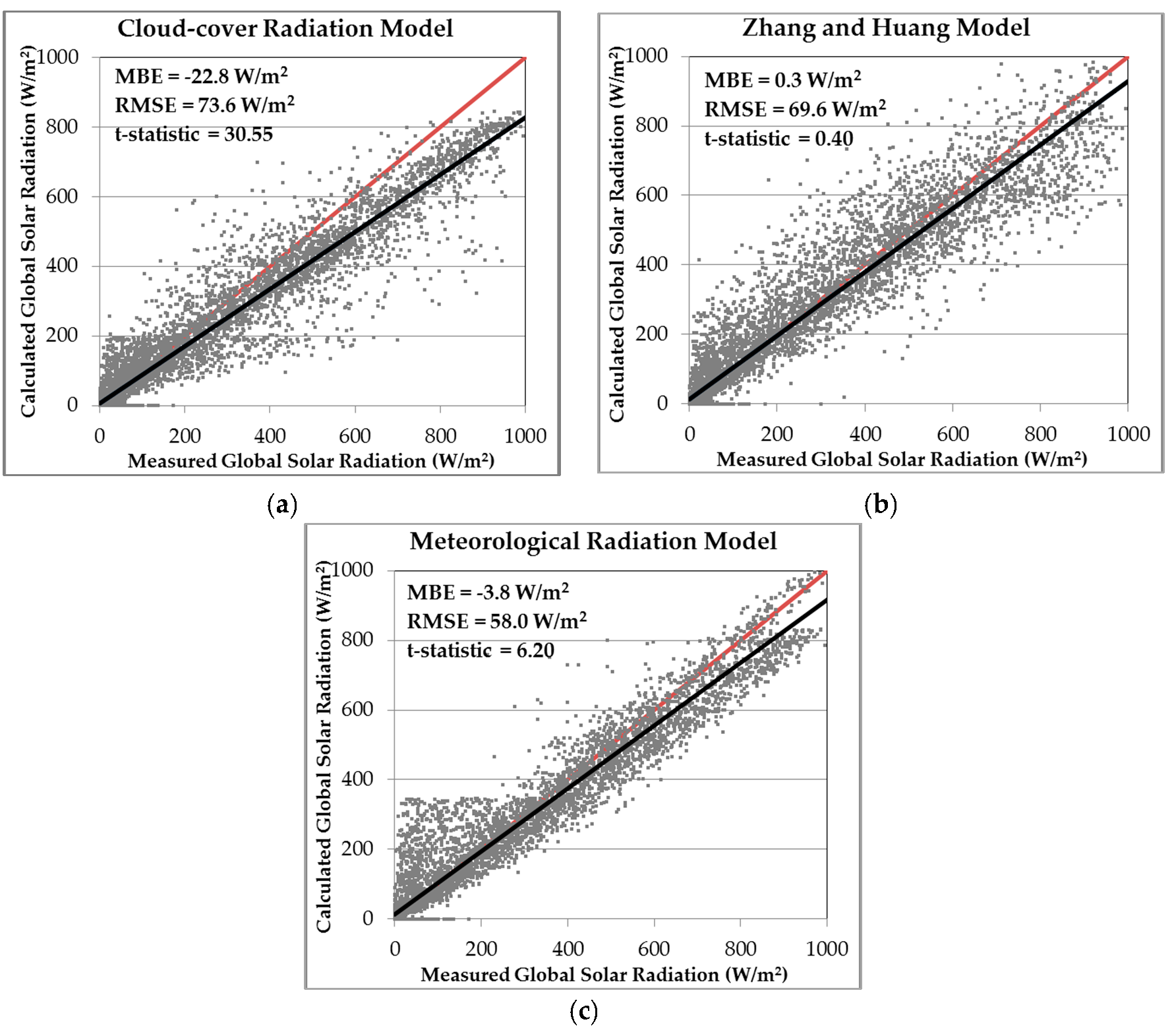
2.1.1. Cloud-Cover Radiation Model (CRM)

The cloud-cover radiation model (CRM), developed by Kasten and Czeplak [3], is a regression-type model that predicts global solar radiation on an hourly basis. To develop this model, ten years of measured solar radiation data and cloud amounts in Hamburg, Germany were collected, and their correlation was used to analyze and calculate site-specific coefficients that could later be employed for calculating solar radiation. It was expanded to other areas by Gul et al. [15] and Muneer and Gul [16] by calculating site-specific coefficients for other cities in Germany. This model has been widely used in a number of different locations around the world because it has an easy calculation process and predicts reliable global solar radiation.
In this model, site-specific coefficients are calculated by a correlation between cloud amount and the corresponding solar altitude angle at that point. Cloud amount is usually divided into nine classes, according to the amount of clouds in the sky (i.e., from 0 oktas for a clear sky to 8 oktas for an overcast sky). However, the KMA measures cloud amount by eleven classes (i.e., from 0 for a clear sky to 10 for an overcast sky), so the original calculation formula was modified to fit the class used in South Korea. In addition, for the site-specific coefficients in Busan, values were obtained from a previous study conducted by Yoo et al. [17]. The modified calculation formula is shown in Equations (1) and (2); A = 930, B = 64, C = 0.77, and D = 2.9 were used as site-specific coefficients.
I g c = A   sin   α B
I g = I g c { 1 C ( N / 10 ) D }

2.1.2. Zhang and Huang Model (ZHM)

The Zhang and Huang Model (ZHM) [4] is a regression-type model that predicts global solar radiation using site-specific coefficients derived from the last three years of measured weather parameters in Beijing and Guangzhou, China, including global solar radiation, dry-bulb temperature, relative humidity, wind speed, and cloud amount. Equation (3) shows the calculation for this model. Since Busan, South Korea (N 35.1°), is located between the latitudes of Beijing (N 39.9°) and Guangzhou (N 23.1°), these cities’ site-specific coefficients were used to calculate the solar radiation in Busan. These were as follows: c0 = 0.5598, c1 = 0.4982, c2 = −0.6762, c3 = 0.02842, c4 = −0.00317, c5 = 0.014, d = −17.853, and k = 0.843. In addition, when the calculated solar radiation was lower than 0, the solar radiation was set to 0, according to the equation:
I g = [ I o s i n α c 0 + c 1 ( N / 10 ) + c 2 ( N / 10 ) 2 + c 3 ( T n T n 3 ) + c 4 Φ + c 5 V W + d ] / k

2.1.3. Meteorological Radiation Model (MRM)

The meteorological radiation model (MRM) [5] developed by Kambezidis and Psiloglou is a mechanistic-type model that predicts global horizontal solar radiation and direct normal solar radiation on an hourly basis. In this model, meteorological data, including sunshine duration, cloud amount, dry- and wet-bulb temperatures, and atmospheric pressure are used for the predictions. This model forecasts global solar radiation for clear and overcast skies by calculating the conditions of atmospheric constituents that cause the absorption and scattering of extraterrestrial radiation on the way to the surface of the Earth. The MRM has a difficult calculation process, but its accuracy has been validated through various weather conditions in countries across Europe and Asia, such as the UK and Japan. Since the entire calculation process is too complicated for this research, only the main equations are shown here. For more detail, please see the study conducted by Psiloglou and Kambezidis [18].
In this model, global solar radiation from a clear sky (Ig-c) can be predicted from the direct solar radiation from a clear sky (Ib-c), calculated by Equation (4), and diffuse solar radiation from a clear sky (Id-c) calculated by Equations (5)–(7). Moreover, diffuse solar radiation (Id-c) consists of circumsolar diffuse radiation, as calculated by a single-scattering model of molecules and aerosols (Ids-c), and diffuse radiation reflected by the ground and backscattered by the atmosphere (Idm-c).
I b c = I e c o s θ z τ w τ r τ o τ m g τ a
I d s c = I e c o s θ z τ w τ o τ m g τ a a 0.5 ( 1 τ a s τ r )
I d m c = ( I b c + I d s c ) ( α g α s ) / ( 1 α g α s )
I d c = I d s c + I d m c
I g c = I b c + I d c
In Equations (4) and (5), Ie is the normal extraterrestrial solar radiation; τ is the broadband transmission functions for water vapor (τw), Rayleigh scattering (τr), uniformly mixed gasses absorption (τmg), and aerosol total extinction (τa); and τaa and τas are the aerosol transmittance functions due to absorption alone and the aerosol transmittance due to scattering alone, respectively. In Equation (6), αg and αs are the surface albedo and albedo of a clear sky, respectively.
Similar to the previous formula, global solar radiation for an overcast sky (Ig) can be predicted from direct solar radiation for an overcast sky (Ib) as calculated by Equation (9), and diffuse solar radiation for an overcast sky (Id) as calculated by Equations (10)–(12).
I b = I b c T c
I d s = I d s c T c + k * ( 1 T c ) ( I b c + I d s c )
I d m = ( I b + I d s ) ( α g α s ) / ( 1 α g α s )
I d = I d s + I d m
I g = I b + I d
In Equation (9), Tc is the cloud transmittance, and in Equation (10), k* is an empirical transmission coefficient according to the latitude of the area.

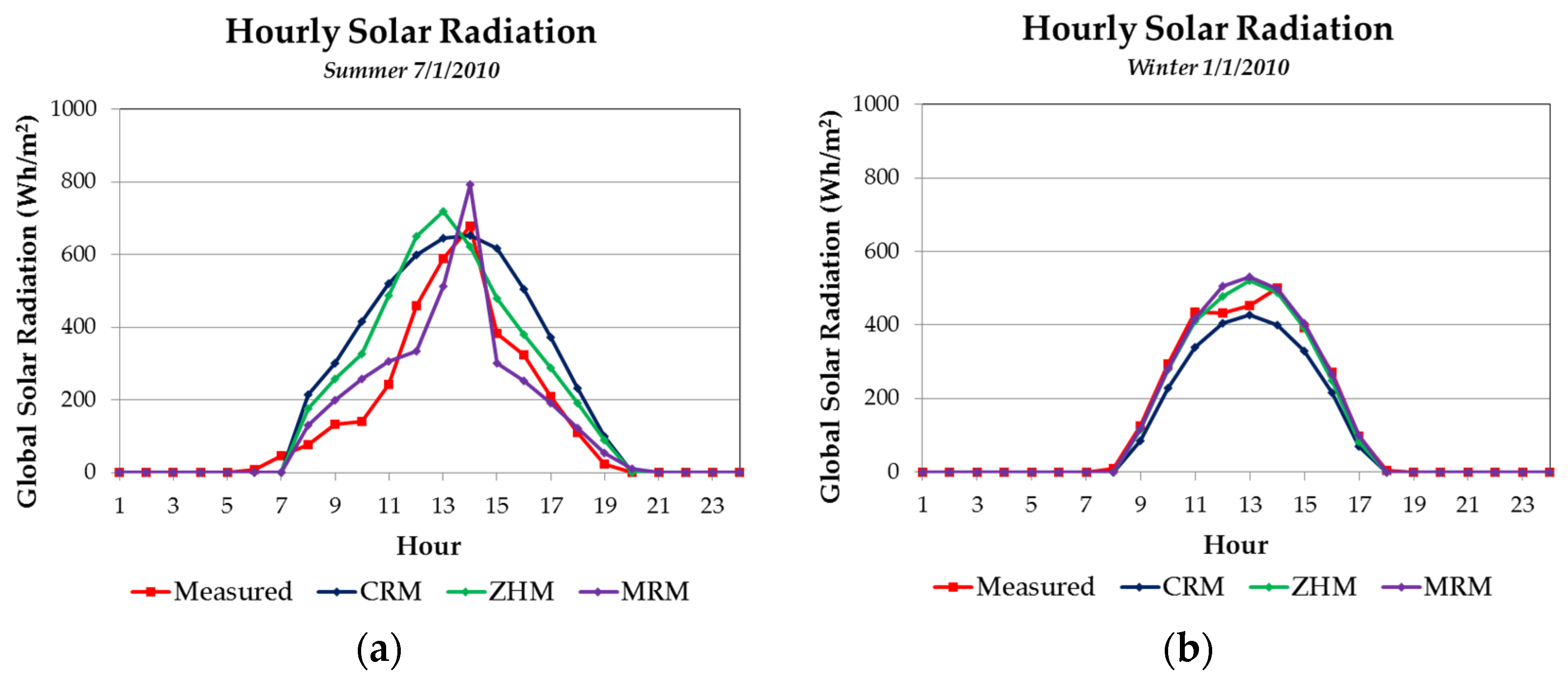
2.2. Global Solar Radiation Results Obtained Using the Three Solar Models

In order to compare the accuracy of the solar models to the calculated and measured global solar radiation, the statistical indices, mean bias error (MBE), root mean square error (RMSE), and t-statistics [19] were reviewed. Equations (14)-(16) show the equations for MBE, RMSE, and t-statistic, respectively. MBE can be used to determine the over or underestimation of the calculated solar radiation, and RMSE can be used to figure out the degree of dispersion of the calculated solar radiation against the measured solar radiation. However, it can be difficult to evaluate the adequacy of the solar models when using more than one index. For example, when the MBE and RMSE show conflicting results (i.e., a high MBE but low RMSE), it is difficult to evaluate the adequacy of the solar model. Thus, a t-statistic that uses both indices was employed to evaluate the solar radiation models in this study.
M B E = ( I I m ) / n
R M S E = ( I I m ) 2 / n
t s t a t i s t i c = [ ( n 1 ) M B E 2 / ( R M S E 2 M B E 2 ) ] 1 / 2
Figure 1 presents the results of the calculated solar radiation using (a) CRM, (b) ZHM, and (c) MRM against the measured solar radiation, along with the MBE, RMSE, and t-statistic indices, and Figure 2 presents the solar radiation by measured and calculated using the three different solar models for a representative day in (a) summer and (b) winter.
As shown in Figure 1, the calculated solar radiation using CRM tends to have an adequate degree of dispersion, but it is unsatisfactorily underestimated as compared to the measured solar radiation. The calculated solar radiation using ZHM tends to have an adequate degree of dispersion and average solar radiation as compared to the measured solar radiation, and the calculated solar radiation using MRM tends to have a unique distribution that has divergent predictions at high levels of solar radiation and inaccurate predictions at solar radiation levels under 300 W/m2. CRM’s underestimation of the calculated solar radiation seems to be caused by using lower site-specific coefficients for the Busan area; MRM’s divergent predictions of the calculated solar radiation seem to be caused by seasonal deviations. In sum, ZHM was the most appropriate solar model with a 0.4 t-statistic, followed by MRM (with a 6.2 t-statistic) and CRM (with a 30.6 t-statistic) throughout a single year, according to the t-statistics index.
In Figure 2a, MRM seems to have a closer tendency on an hourly basis to the measured solar radiation, followed by ZHM and CRM for a representative day in summer, and in Figure 2b, ZHM and MRM seem to have a closer tendency on an hourly basis to the measured solar radiation, followed by CRM for a representative day in winter.
In this research, solar radiation was compared to facilitate a more detailed analysis of solar radiation prediction models. Table 1 shows the t-statistics of the monthly and annual solar radiation for each model. According to these monthly t-statistics, MRM was the closest to the measured solar radiation for the most months (January, February, March, April, June, July, August, September, and December), and ZHM was closest to the measured solar radiation for the other months (May, October, and November). These results are attributable to the weather parameters used in each solar model. CRM calculates solar radiation from only one weather parameter, cloud amount, but ZHM uses dry-bulb temperature, relative humidity, and wind speed, in addition to cloud amount. Moreover, MRM uses sunshine duration, dry- and wet-bulb temperature, and atmospheric pressure, along with cloud amount, so it reflects the influence of the absorption and scattering of solar radiation by the atmosphere.
From an analysis of annual solar radiation using t-statistics, ZHM was selected as the most appropriate solar model for the Busan area; however, from an analysis of the monthly solar radiation, the calculated solar radiation was found to have seasonal variations in extreme weather, such as summer and winter, as also shown in Figure 2a. Thus, a new solar model must be developed so that, in the future, these seasonal characteristics can be included.

2.3. An Office Building’s Energy Performance using Calculated Solar Models

2.3.1. Actual Meteorological Year (AMY) Weather File

(1)
Weather parameters
Since the final goal of this study was to develop a new solar model that would be appropriate for areas in South Korea in order to improve building energy performance analysis, a weather file required for running building energy simulation programs was created. In order to pack this weather file, the measured weather data for 2010, including hourly dry-bulb, wet-bulb, and dew-point temperatures, wind speed and direction, atmospheric pressure, and global horizontal solar radiation were collected from a weather station in Busan, South Korea (latitude N 35.1°, longitude 129.02°, altitude 69.6 m). However, there were no data for direct normal solar radiation from this weather station. Instead, they were calculated by applying the measured global solar radiation to Erbs equations [20], shown in Equations (17)–(22). Equation (17) is applicable when the clearness index (kT) is lower than 0.22, Equation (18) is applicable when the clearness index (kT) is between 0.22 and 0.8, and Equation (19) is applicable when the clearness index (kT) is higher than 0.8.
I d / I g = 1.0 0.09 k T
I d / I g = 0.9511 0.1604 k T + 4.388 k 2 T 16.638 k 3 T + 12.336 k 4 T
I d / I g = 0.165
I e = I o { 1 + 0.033 c o s ( 360 n / 365 ) } × ( c o s Φ c o s δ c o s ω + s i n Φ s i n δ )
I d = ( I d / I g ) × I g
I b = { 1 ( I d / I g ) } × I g
(2)
Packing Actual Meteorological Year (AMY) weather files
Using the weather data obtained from the weather station and calculations mentioned above, an actual meteorological year (AMY) weather file was packed to build an energy simulation. In this study, four weather files were packed, each containing the same weather parameters, except for four different global solar radiation data (i.e., one was measured solar radiation, and the others were solar radiation calculated by CRM, ZHM, and MRM). The four weather files are summarized in Table 2.
To pack the AMY-formatted weather file, the packing procedures developed by the Lawrence Berkeley National Laboratory (LBNL), USA were applied [21]. In order to pack an AMY weather file, the DOE-2.2/eQUEST program requires two types of input files: TPE and INP. A TPE file contains all of the weather parameter data mentioned above; an INP file contains characteristics information, including the year the weather data were measured, identification number of the weather station, local geometry information, such as latitude and longitude, monthly clearness index, and so on. Most importantly, an INP file requires the average monthly clearness index measured at the weather station. For this research, the average monthly data were calculated by the measured daily clearness index at the weather station in 2010. Using these two input files, the AMY weather files were packed by the DOE-2.1e program.

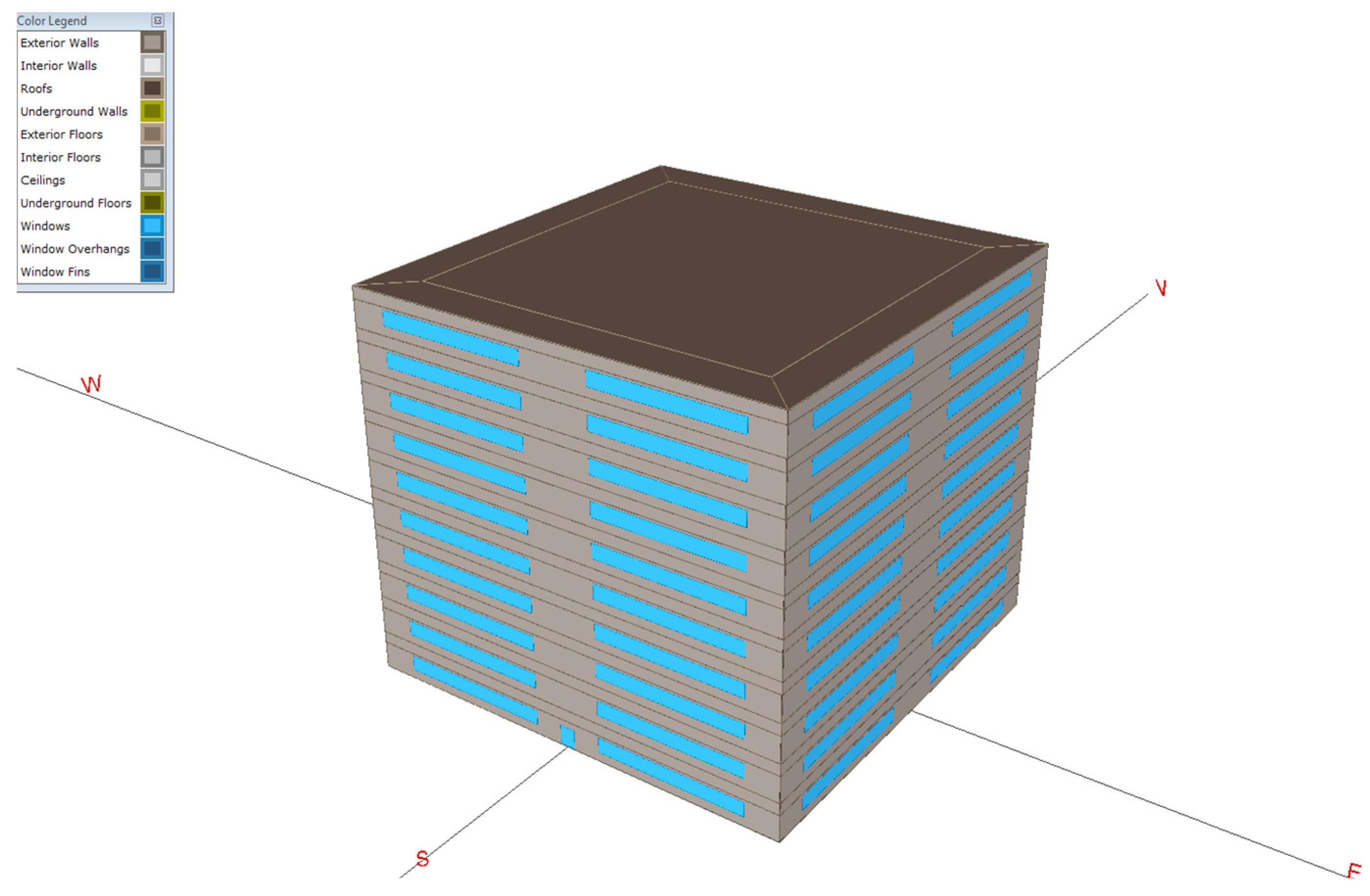
2.3.2. Analysis of an Office Building’s Energy Performance

(1)
Building Energy Simulation Program
For decades, the DOE-2.2/eQUEST program [22] has been acknowledged as one of the best programs in the field of building energy performance analysis; thus, for this research it was used to model an office building in Busan, South Korea where has a warm and marine climate according to ASHRAE Standard 90.1-2007 [23] with 1972 HDD18 and 2418 CDD10. A ten story standard office building with 2323 m2 of floor area on each floor was created. The input information for the building envelope is shown in Table 3, and the HVAC systems are listed in Table 4. The inputs for the tables were determined according to the following criteria: the thermal transmittance of the building envelope’s components were set to be compliant with the “Design Standard Guideline for Building Energy Saving” [24] developed by the Korea Energy Agency (KEA), and the air infiltration rate was set according to suggestions made by the US Pacific Northwest National Laboratory (PNNL) [25]. Moreover, operational schedules proposed by the US National Renewable Energy Laboratory (NREL) [26] were applied to the simulation, including internal load, lighting and equipment power density, schedules for occupants, lighting, appliances, temperatures for heating and cooling systems, ventilation, and hot water heaters. As shown in Figure 3, the office building was of a square type with even 28% window-to-wall ratio (WWR) in all directions.
Next, in order to identify the effects of differences in the global solar radiation values determined by separate solar models on a standard office building’s energy performance, several simulations were run after the following window characteristics were changed: solar heat gain coefficient (SHGC) and window-to-wall ratio (WWR). Initially, the window characteristics were set to 0.4 SHGC and 28% WWR in all directions. Then, the WWR was changed to 30% and 50%, and the SHGC was changed to 0.6 and 0.8. The variation range for the WWR was set to have maximum 50% because of the recommendation from the “Design Standard Guideline for Building Energy Saving” [24] for public office buildings, and the variation range for the SHGC was set to cover various type of windows from high reflective coating glass to uncoated clear glass, which have been installed in most office buildings in South Korea. All of the simulation cases were run using four different weather files with different global solar radiation levels, and the resulting building energy consumptions were compared and analyzed.
(2)
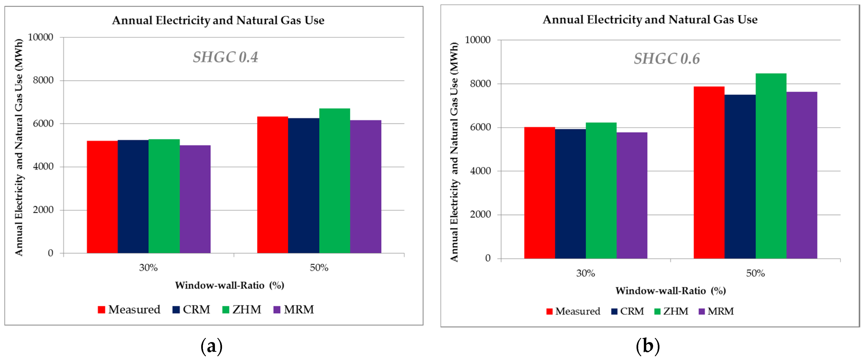
Results of the Building Energy Performance Analysis
Figure 4 presents the annual energy consumptions for the standard office building using four different weather files after changing the SHGC and WWR. Figure 4a shows the annual energy consumptions simulated by the four different weather files when the WWR values were 30% and 50%, and the SHGC was 0.4; Figure 4b shows the annual energy consumption when the SHGC was 0.6; and Figure 4c shows the annual energy consumption when the SHGC was 0.8.
When the windows had a low SHGC (i.e., 0.4), the annual energy consumption of the office building increased gradually by 19%, from 5200 MWh to 6400 MWh, according to increments of the WWR ranging from 30% to 50% (as shown in Figure 4a), but when the windows had a higher SHGC (i.e., 0.6), the annual energy consumption of the building increased rapidly by 24%, from 6000 MWh to 7900 MWh, according to increments of the WWR ranging from 30% to 50% (as shown in Figure 4b). In addition, when the windows had their highest SHGC (i.e., 0.8), the annual energy consumption of the building rapidly increased by 26%, from 6800 MWh to 9200 MWh, according to increments of the WWR ranging from 30% to 50% (as shown in Figure 4c). Thus, this shows that the annual energy consumption of a building increases gradually as the SHGC increases, along with the effect of the particular increment of the WWR.
In addition, when the WWR was 30% and the SHGC increased from 0.4 to 0.6, the annual energy consumption of the building increased by 13%, from 5200 MWh to 6000 MWh. Moreover, the annual energy consumption of the building increased by 13%, from 6000 MWh to 6800 MWh, as the SHGC increased from 0.6 to 0.8. On the other hand, when the WWR was 50%, the annual energy consumption of the building increased by 19%, from 6400 MWh to 7900 MWh, and 14%, from 7900 MWh to 9200 MWh, as the SHGC increased from 0.4 to 0.6 and 0.6 to 0.8, respectively; this shows that the energy consumption decreases as the SHGC increases.
A comparison of the energy consumptions of the building according to the three different solar models showed the following results: when the SHGC and WWR were low (i.e., the SHGC was 0.4 and WWR was 30%), the percentage differences among the solar models were small, ranging from −0.6% to 4.0%. However, the percentage differences increased significantly, ranging from 4% to 8%, when the SHGC and WWR were high (i.e., the SHGC was 0.8 and WWR was 50%).
Next, in order to identify the most area-appropriate solar models for improving office building energy performance analysis, the monthly energy consumptions of the building according to the SHGC and WWR variations were analyzed. Table 5 and Table 6 present the month-by-month percentage differences in energy consumptions between those predicted using solar radiation determined by the three different solar models and those determined using measured solar radiation. The values highlighted in grey in the table indicate the solar models that come closest to using measured solar radiation.
The case with a 30% WWR illustrates that there were differences for each month, but the energy consumptions of the building determined through CRM (in June, July, August, September, October, and November) and ZHM (in January, February, March, April, May, and December) were the closest to using measured solar radiation in a low SHGC (i.e., 0.4), whereas the energy consumptions of the building determined through CRM (in January, February, March, April, November, and December) and MRM (in May, June, July, August., September, and October) were the closest to using measured solar radiation in a high SHGC (i.e., 0.8). In addition, the case with a 50% WWR shows that the energy consumptions of the building determined through CRM (in January, February, March, April, May, September, November, and December) were the closest to using measured solar radiation for most of the month in a low SHGC (i.e., 0.4), whereas the energy consumptions of the building determined through MRM (in April, May, June, July, August, September, October, November, and December) were the closest to using measured solar radiation in a high SHGC (i.e., 0.8). To sum up the results, CRM and ZHM were shown to be appropriate models for the office building when there were low WWR and SHGC, and MRM was comparatively better when the WWR and SHGC were high.
This analysis of building energy consumption is also consistent with earlier results using calculated solar radiation obtained from the three different solar models. In calculations of global solar radiation using the solar models, ZHM (with a 0.4 t-statistic) was the most adequate, and MRM (with a 6.2 t-statistic) and CRM (with a 30.6 t-statistic) followed, according to the t-statistic. On the other hand, in the analysis of monthly solar radiation, MRM was the most appropriate model for most of the months (January, February, March, April, June, July, August, September, and December), and ZHM was best during the other months (May, October, and November). For hourly solar radiation, the solar radiation calculated by MRM was more proximate to the measured solar radiation, except when the solar radiation was below 300 W/m2; ZHM showed the approximate average solar radiation, but had a higher degree of dispersion than MRM.
Due to the nature of building energy simulation programs that calculate energy consumption on an hourly basis, one can conclude from the above analyses that using MRM for building energy performance may be better for reducing errors than using ZHM. In addition, this research provides meaningful information regarding how important it is to accurately predict hourly fluctuations in solar radiation when attempting to improve building energy performance analysis.

3. Discussion and Conclusions

In this study, a quantitative comparative analysis of an office building energy performance was conducted using four different weather files containing hourly measured global solar radiation and hourly solar radiation calculated through three different solar models: CRM, ZHM, and MRM. The findings from this study can be summarized as follows:
(1)
The hourly global solar radiation in Busan, South Korea in 2010 was calculated using three different solar models (i.e., CRM, ZHM, and MRM) and compared to the measured solar radiation. As a result, ZHM was selected as the most accurate model in this area, generally, but it showed significant differences from the measured data in extreme seasonal conditions, such as those that occur in summer and winter. Thus, the model should be improved by considering seasonal characteristics, which could be accomplished by using additional weather parameters, such as sunshine duration, atmospheric pressure, and so on (similar to those that were used in MRM).
(2)
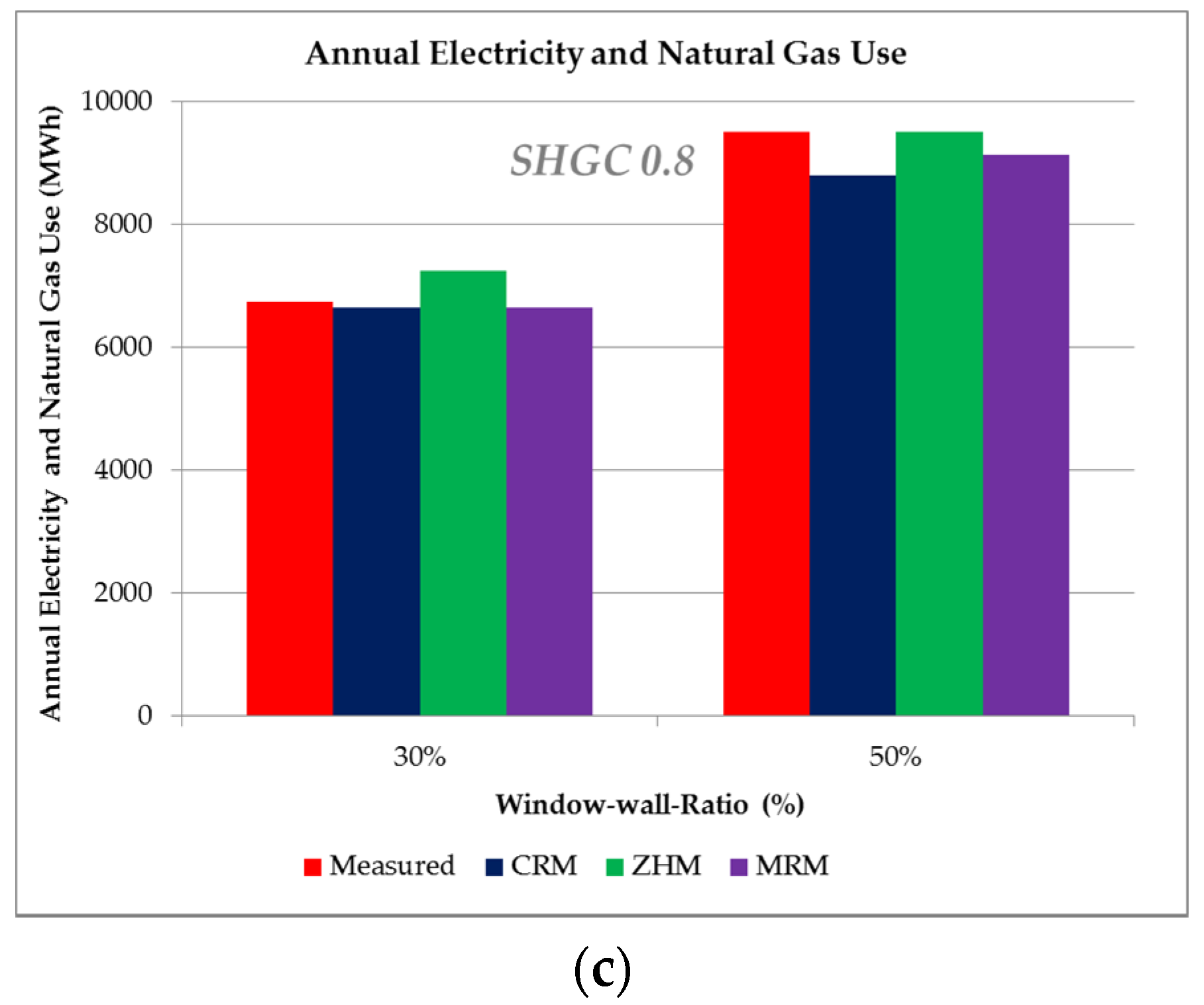
In the office building energy performance, when the effect of global solar radiation was small (i.e., when the building had low SHGC and WWR), the differences in energy consumption between using the measured solar radiation and the solar radiation calculated from the solar models were small, ranging from −0.6% to 4%, but the differences increased up to 8% as the SHGC and WWR increased.
(3)
The most accurate solar models (according to changes in the SHGC and WWR) were as follows: CRM and ZHM were shown to be the most accurate if the office building had low SHGC and WWR (i.e., 0.4 and 30%, respectively), and MRM was the most accurate in high SHGC and WWR (i.e., 0.8 and 50%, respectively).
(4)
Variations in the building energy simulation results could be caused by the weather parameters used in the solar models. CRM calculates global solar radiation using only one weather parameter, cloud amount, but MRM uses sunshine duration, dry- and wet-bulb temperatures, atmospheric pressure, and cloud amount to determine the influence of the absorption and scattering of the solar radiation in the atmosphere.
(5)
The analysis results imply the necessity of the following considerations when performing a building energy analysis using calculated solar radiation: it is important to predict solar radiation to have a closer tendency on an hourly basis to the measured solar radiation when applying it to building energy simulation programs, although more case studies should be considered in the future work, including varying other window characteristics, such as U-value and visible transmittance, etc., and other building envelope characteristics. In addition, to improve building energy performance analyses, the accuracy of calculated solar radiation should be improved through the consideration of seasonal characteristics. Therefore, a new solar model for South Korea that applies the findings from this study should be developed; it will improve future building energy performance analyses.

Acknowledgments

This work was supported by the National Research Foundation of Korea (NRF) grant funded by the Korea government (MSIP) (No. 2016R1C1B2014542).

Author Contributions

Kee Han Kim design and wrote the paper; John Kie-Whan Oh provided comprehensive discussion; WoonSeong Jeong discussed the main idea to develop this research work and reviewed and revised the paper.

Conflicts of Interest

The authors declare no conflicts of interest.

Abbreviations

The following abbreviations are used in this manuscript:
Im
Measured Hourly Global Solar Radiation (W/m2)
Io
Solar Constant (1366 W/m2)
Ie
Extraterrestrial Solar Radiation (W/m2)
Ig
Calculated Hourly Global Solar Radiation (W/m2)
Ib
Calculated Hourly Direct Solar Radiation (W/m2)
Id
Calculated Hourly Diffuse Solar Radiation (W/m2)
Ids
Circumsolar Diffuse Radiation by a Single-scattering Mode of Molecules and Aerosols (W/m2)
Idm
Diffuse Radiation Reflected by the Ground and Backscattered by the Atmosphere (W/m2)
Ig-c
Calculated Hourly Global Solar Radiation for a clear sky (W/m2)
Ib-c
Calculated Hourly Direct Solar Radiation for a clear sky (W/m2)
Id-c
Calculated Hourly Diffuse Solar Radiation for clear sky (W/m2)
α
Solar Altitude Angle (m)
θz
Zenith Angle (degree)
N
Cloud Amount (0–10 okta)
n
Number of Data Points
Φ
Relative Humidity (%)
Tn, Tn-3
Dry-bulb Temperature in Celsius at hours n and (n-3), respectively
Vw
Wind Speed (m/s)
τ
Optical Transmittance
αg, αs
Albedo of the Surface and the Clear Sky

References

  1. Korea Meteorological Administration. Available online: http://www.kma.go.kr/index.jsp (accessed on 13 June 2010).
  2. Lee, K.; Sim, K. Analysis and calculation of global hourly solar irradiation based on sunshine duration for major cities in Korea. J. Korean Sol. Energy Soc. 2010, 30, 16–21. (In Korean) [Google Scholar]
  3. Kasten, F.; Czeplak, G. Solar and terrestrial radiation dependent on the amount and type of cloud. Sol. Energy 1980, 24, 177–189. [Google Scholar] [CrossRef]
  4. Zhang, Q.; Huang, Y. Development of typical year weather files for Chinese locations. ASHRAE Trans. 2002, 108, 1063–1075. [Google Scholar]
  5. Kambezidis, H.; Psiloglou, B. The Meteorological Radiation Model (MRM): Advancements and Applications. In Modeling Solar Radiation at the Earth’s Surface; Springer: Berlin, Germany, 2008. [Google Scholar]
  6. Yang, K.; Koike, T. Estimating surface solar radiation from upper-air humidity. Sol. Energy 2002, 77, 177–186. [Google Scholar] [CrossRef]
  7. Perez, R.; Ineichen, K.; Moore, K.; Kmiecik, M.; Chain, C.; George, R.; Vignola, F. A new operational model for satellite-derived irradiances: description and validation. Sol. Energy 2002, 73, 307–317. [Google Scholar] [CrossRef]
  8. Perez, R.; Moore, M.; Wilcox, S.; Renne, D.; Zelenka, K. Forecasting solar radiation: preliminary evaluation of an approach based upon the National Forecast Database. Sol. Energy 2007, 81, 809–812. [Google Scholar] [CrossRef]
  9. Zelenka, A.; Perez, R.; Seals, R.; Renne, D. Effective accuracy of the satellite-derived hourly irradiance. Theor. Appl. Climatol. 1999, 62, 199–207. [Google Scholar]
  10. HelioClim. HelioClim: Providing Information on Solar Radiation; Centre Energetique et Procedes of Ecole des Miners de Paris. Available online: http://www.helioclim.org/heliosat/index.html (accessed on 19 June 2016).
  11. Janjai, S.; Laksanaboonsong, J.; Nunez, M.; Thongsathitya, A. Development of a method for generating operational solar radiation maps from satellite data for a tropical environment. Sol. Energy 2005, 78, 739–751. [Google Scholar] [CrossRef]
  12. Krarti, M.; Hunag, J.; Seo, D.; Dark, J. Development of Solar Radiation Models for Tropical Locations, ASHRAE Project RP-1309; ASHRAE: Atlanta, GA, USA, 2006. [Google Scholar]
  13. Seo, D.; Krarti, M. Impact of solar models on building energy analysis for tropical sites. ASHRAE Trans. 2007, 113, 523–530. [Google Scholar]
  14. Wan, K.; Cheung, K.; Liu, D.; Lam, J.C. Impact of modelled global solar radiation on simulated building heating and cooling loads. Energy Convers. Manag. 2009, 50, 662–667. [Google Scholar] [CrossRef]
  15. Gul, M.; Muneer, T.; Kambezidis, H. Models for obtaining solar radiation from other meteorological data. Sol. Energy 1998, 64, 99–108. [Google Scholar] [CrossRef]
  16. Muneer, T.; Gul, M. Evaluation of sunshine and cloud cover based models for generating solar radiation data. Energy Convers. Manag. 2000, 41, 461–482. [Google Scholar] [CrossRef]
  17. Yoo, H.; Lee, K.; Park, S. Analysis of data and calculation of global solar radiation based on cloud data for major cities in Korea. J. Korean Sol. Energy Soc. 2008, 28, 17–24. (In Korean) [Google Scholar]
  18. Psiloglou, B.; Kambezidis, H. Performance of the meteorological radiation model during the solar eclipse of 29 of March 2006. Atmos. Chem. Phys. Discuss. 2007, 7, 6047–6059. [Google Scholar] [CrossRef]
  19. Stone, R. Improved statistical procedure for the evaluation of solar radiation estimation models. Sol. Energy 1993, 51, 289–291. [Google Scholar] [CrossRef]
  20. Duffie, J.; Beckman, W. Solar Engineering of Thermal Processes, 2nd ed.; John Wiley & Sons, Inc.: Hoboken, NJ, USA, 2006. [Google Scholar]
  21. Buhl, F. Weather Processor; Lawrence Berkeley National Laboratory: Berkeley, CA, USA, 1999. [Google Scholar]
  22. LBNL. DOE-2.2 Building Energy Use and Cost Analysis Program, Volume 1: Basics; Lawrence Berkeley National Laboratory: Berkeley, CA, USA, 2004. [Google Scholar]
  23. ASHRAE. ASHRAE Standard 90.1–2007; American Society of Heating, Refrigeration, and Air-Conditioning Engineers: Atlanta, GA, USA, 2007. [Google Scholar]
  24. Korea Energy Agency. Design Standard Guideline for Building Energy Saving; Korea Energy Agency: Gyeonggi-do, Korea, 2011. (In Korean) [Google Scholar]
  25. Gowri, K.; Winiarski, D.; Jarnagin, R. Infiltration Modeling Guidelines for Commercial Building Energy Analysis, PNNL-18898; Pacific Northwest National Laboratory: Washington, DC, USA, 2009. [Google Scholar]
  26. Deru, M. Energy Savings Modeling and Inspection Guidelines for Commercial Building Federal Tax Deductions; National Renewable Energy Laboratory: Golden, CO, USA, 2007. [Google Scholar]
Figure 1. Calculated global solar radiation against measured global solar radiation using three different solar models: (a) cloud-cover radiation model; (b) Zhang and Huang model; and (c) meteorological radiation model.
Sustainability 08 00589 g001
Figure 2. Solar radiation by measured and calculated using the three different solar models for a representative day in (a) summer; and (b) winter.
Sustainability 08 00589 g002
Figure 3. Office building modeled by DOE-2.2/eQUEST.
Sustainability 08 00589 g003
Figure 4. Simulated annual energy use using four different values of solar radiation data: (a) when the SHGC was 0.4; (b) 0.6; and (c) 0.8.
Sustainability 08 00589 g004aSustainability 08 00589 g004b
Table 1. Comparison of the t-statistics index of monthly global solar radiation derived from three different models (the most accurate model is highlighted in grey).
ModelJan.Feb.Mar.Apr.MayJun.Jul.Aug.Sept.Oct.Nov.Dec.Ann.
CRM2.511.821.311.851.501.581.401.802.022.532.542.106.23
ZHM0.991.051.640.960.020.460.941.711.210.570.721.100.08
MRM0.980.351.010.240.100.380.600.990.881.831.060.221.26
Table 2. Summary of four different weather files.
Weather ParametersWeatherWeatherWeatherWeather
File #1File #2File #3File #4
Dry-bulb TemperatureWeather Sta.Weather Sta.Weather Sta.Weather Sta.
Wet-bulb TemperatureWeather Sta.Weather Sta.Weather Sta.Weather Sta.
Dew-point TemperatureWeather Sta.Weather Sta.Weather Sta.Weather Sta.
Wind SpeedWeather Sta.Weather Sta.Weather Sta.Weather Sta.
Wind DirectionWeather Sta.Weather Sta.Weather Sta.Weather Sta.
Atmospheric PressureWeather Sta.Weather Sta.Weather Sta.Weather Sta.
Global Solar RadiationMeasuredCRMZHMMRM
Direct Normal Solar RadiationCalculated by Erbs using measuredCalculated by Erbs using measuredCalculated by Erbs using measuredCalculated by Erbs using measured
Table 3. Description of office building model.
CategoryInputValue
GeneralFloor area (m2)2323
Number of floors10
Window-to-wall ratio (%)28
Floor-to-ceiling height (m)2.7
Exterior wallU-factor (W/m2·K)0.45
RoofU-factor (W/m2·K)0.24
Slab-on-grade floorU-factor (W/m2·K)0.58
Window/DoorU-factor (W/m2·K)2.70
Solar Heat Gain Coefficient0.40
Air infiltration (m3/hr·m2)2.19
Internal loadArea/Person (m2)9.3
People load (W)117.2
Lighting density (W/m2)12.92
Equipment density (W/m2)16.15
Table 4. Description of HVAC systems in office building model.
SystemTypeInput and value
HVAC-SD VAV w/reheat
PlantChiller efficiencySEER 13
Boiler efficiency (%)86.5%
Service water heater efficiencyEF 0.93
Table 5. Comparison of percentage differences (%) in office building energy consumptions using three different weather files when the WWR was 30% and the SHGC changed from 0.4 to 0.8 (the most accurate model is highlighted in grey).
SHGCModelJan.Feb.Mar.Apr.MayJun.Jul.Aug.Sep.Oct.Nov.Dec.Ann.
0.4CRM1.81.62.21.0−0.60.3−0.4−0.81.0−0.41.31.30.6
ZHM0.90.20.40.90.22.93.02.02.41.71.80.71.5
MRM−3.7−4.4−3.9−4.8−5.5−4.1−2.8−3.1−3.3−4.7−5.1−4.6−4.0
0.6CRM1.6−0.40.2−1.3−3.3−2.4−3.5−3.8−1.3−2.3−0.9−0.5−1.6
ZHM3.02.11.92.41.64.93.93.14.54.53.62.63.3
MRM−4.0−4.5−4.5−4.9−5.4−3.5−3.6−3.1−2.9−3.4−4.9−4.8−4.0
0.8CRM1.6−1.00.2−1.0−2.8−2.0−3.3−3.3−0.7−1.6−0.6−0.3−1.4
ZHM6.44.65.15.85.38.87.86.88.78.77.26.06.9
MRM−2.8−3.4−2.8−2.8−2.7−0.5−0.6−0.50.3−0.3−2.5−3.2−1.6
Table 6. Comparison of percentage differences (%) in office building energy consumptions using three different weather files when the WWR was 50% and the SHGC was changed from 0.4 to 0.8 (the most accurate model is highlighted in grey).
SHGCModelJan.Feb.Mar.Apr.MayJun.Jul.Aug.Sep.Oct.Nov.Dec.Ann.
0.4CRM1.70.00.4−1.0−2.7−2.2−3.5−3.8−1.1−1.7−0.1−0.4−1.3
ZHM4.64.23.94.64.37.46.45.27.17.46.34.65.6
MRM−3.2−3.4−3.2−3.6−3.7−1.9−2.1−2.4−1.4−1.5−3.3−3.6−2.7
0.6CRM−1.6−4.2−3.1−4.8−6.6−6.4−7.7−7.5−5.0−5.2−3.6−3.4−5.2
ZHM6.74.85.15.65.48.77.86.98.69.27.56.27.0
MRM−4.3−4.9−4.6−4.8−4.6−2.4−2.4−2.0−1.6−1.6−3.9−4.7−3.3
0.8CRM−4.2−7.5−5.8−7.7−9.59.4−11.0−11.0−8.1−7.9−6.3−6.2−8.1
ZHM6.64.45.25.95.89.28.17.18.89.97.96.37.3
MRM−5.5−6.1−5.7−5.8−5.4−3.1−3.0−2.3−2.3−2.1−4.8−5.6−4.0

