Urbanization and Its Effects on Industrial Pollutant Emissions: An Empirical Study of a Chinese Case with the Spatial Panel Model

Abstract

Urbanization is considered a main indicator of regional economic development due to its positive effect on promoting industrial development; however, many regions, especially developing countries, have troubled in its negative effect—the aggravating environmental pollution. Many researchers have addressed that the rapid urbanization stimulated the expansion of the industrial production and increased the industrial pollutant emissions. However, this statement is exposed to a grave drawback in that urbanization not only expands industrial production but also improves labor productivity and changes industrial structure. To make up this drawback, we first decompose the influence of urbanization impacts on the industrial pollutant emissions into the scale effect, the intensive effect, and the structure effect by using the Kaya Identity and the LMDI Method; second, we perform an empirical study of the three effects by applying the spatial panel model on the basis of the data from 282 prefecture-level cities of China from 2003 to 2014. Our results indicate that (1) there are significant reverse U-shapes between China’s urbanization rate and the volume of industrial wastewater discharge, sulfur dioxide emissions and soot (dust) emissions; (2) the relationship between China’s urbanization and the industrial pollutant emissions depends on the scale effect, the intensive effect and the structure effect jointly. Specifically, the scale effect and the structure effect tend to aggravate the industrial wastewater discharge, the sulfur dioxide emissions and the soot (dust) emissions in China’s cities, while the intensive effect results in decreasing the three types of industrial pollutant emissions; (3) there are significant spatial autocorrelations of the industrial pollutant emissions among China’s cities, but the spatial spillover effect is non-existent or non-significant. We attempt to explain this contradiction due to the fact that the vast rural areas around China’s cities serve as sponge belts and absorb the spatial spillover of the industrial pollutant emissions from cities. According to the results, we argue the decomposition of the three effects is necessary and meaningful, it establishes a cornerstone in understanding the definite relationship between urbanization and industrial pollutant emissions, and effectively contributes to the relative policy making.

1. Introduction

The theme of Shanghai World Expo in 2010—Better City, Better Life—exhibits China’s great ambition for urbanization. In fact, the state of urbanization in China is experiencing much disappointment with the aggravating environmental pollution, which is one of the most serious problems in current China’s cities. The World Bank [1,2] indicated in its reports that since 1978, China’s economy had produced economic growth that rated it one of the fastest growing economies in the world; even though tremendous efforts had been made in abating environmental pollution, China had suffered from an increase of environmental pollution and stern criticism simultaneously.

The deteriorated environment in China has lowered the people’s quality of life, and showing that cities do not bring a better life. Just as Easterlin et al. [3] documented, self-reported life satisfaction indicators were not increased in China as much as the expected 8 percent annual economic growth in a parallel period.

What makes China suffer from such a large number of serious environmental pollution incidents? Vennemo et al. [4] noted that China appeared to be following a path similar to the one trodden by some earlier industrialized countries, and the increase of the industrial pollutant emissions have deteriorated the environmental situation. Furthermore, many researchers stated that the rapid urbanization in China stimulated the expansion of the industrial production, which then generated a great deal of air and water pollutants and consequently resulted to the deterioration of air and water quality. Thus, urbanization aggravates environmental pollution.

However, we hold the opinion that this statement is exposed to a grave drawback. On the one hand, it is true that China’s urbanization expands the industrial production, but on the other hand, the process of urbanization also promotes the industrial labor productivity and upgrades the industrial structure. Even though the expansion of the industrial production will aggravate the industrial pollutant emissions, the improvement of the industrial labor productivity and the upgrading of the industrial structure will relief the increasing trend of industrial pollutant emissions. As a result, the relationship between urbanization and industrial pollutant emissions is ambiguous, which should be considered cautiously.

In this paper, we highlight our research in the following aspects: first, we explore the mechanism analysis between urbanization and industrial pollutant emissions and then apply the Kaya Identity and the LMDI Method to decompose out three effects (i.e., the scale effect, the intensive effect and the structure effect) of the urbanization impacts on the industrial pollutant emissions; second, we elaborate a description of the relationship between urbanization rate and industrial pollutants emissions of China, and re-examine the reverse U-shapes between them, then we perform an empirical study of the three effects on the basis of the data from 282 cities of China from 2003 to 2014; third, as economic developments are strongly related with each other in different regions, and the assumption of no spatial autocorrelations has been questioned by many scholars, we amend the traditional panel model by introducing the spatial panel model to incorporate the spatial spillover effect.

The rest of the paper is arranged as follows: Section 2 briefly reviews the previous studies; Section 3 analyses the mechanisms between urbanization and industrial pollutant emissions; Section 4 establishes the spatial panel model and introduces the parameters; Section 5 presents the empirical analysis; and Section 6 presents the study’s conclusions and offers a discussion.

2. Literature Review

From an early time, understanding the trade-off between the positive and negative externalities of urban growth has been the core issue in urban and environmental economics (Tolley [5], Glaeser [6]). Urbanization is considered as a main indicator of regional economic development due to its positive effect on promoting industrial development, but many regions, especially developing countries, have trouble of its negative effect—the aggravation of environmental pollution (Wan and Wang [7]). The relationship between economic development and environmental pollution has been analyzed by early representative works such as Grossman and Krueger [8,9] and Panayotou [10], which similarly proposed the Environmental Kuznets Curve (i.e., the EKC theory). Based on these influential studies, an entire subfield of environment economics has emerged in focusing on the association between economic and environmental indicators.

One subfield of environment economics studies focuses on the re-examination of the validity of the EKC theory. For example, Lindmark [11], Nasir and Rehman [12], Eeteve and Tamarit [13], Jalil and Mahmud [14], and Li et al. [15] applied Swedish, Pakistani, Spanish and Chinese data to perform empirical tests on the reverse U-shapes between national income per capita and environmental pollution status, and their results strongly supported the EKC theory in various scenarios. However, many other empirical studies, especially those based on time series models, argued that the declining portions of the Environmental Kuznets Curve were illusory, either because they were cross-sectional snapshots that masked a long-run “race to the bottom” in environmental standards or because industrial societies continually produced new pollutants because the old ones were controlled (Stern [16], York et al. [17], Kwon [18]).

Another subfield is the study of the causes of the reverse U-shape in the Environmental Kuznets Curve. Dasgupta et al. [19] suggested that the driving forces of making the Environmental Kuznets Curve flatten and shift to the right appeared to be the economic liberalization, clean technology diffusion, and new approaches to pollution regulation. Panayotou [20] proposed another visualized explanation based on the decomposition of the influence of economic development on environmental pollution into three effects: the scale effect, the technology effect and the composition effect. He noted that the reverse U-shape of EKC was the comprehensive impact of the three effects.

In terms of the relationship between urbanization and industrial pollutant emissions, Kanada et al. [21], Qin et al. [22], and Dong et al. [23] studied the way in which urban population growth impacted local pollution levels and indicated that as the urban population became richer, the demand of private transportation and electricity sharply increased; thus, the activities and demands of individuals exacerbated urban pollution externalities. However, Tao et al. [24] obtained an opposite result arguing that the overall quantity of pollutant discharge decreased as cities became more economically developed during the period from 2000 to 2010, and they attributed such positive effect to higher urban production efficiencies. Zhou et al. [25] used the STIRPAT model (Stochastic Impacts by Regression on Population, Affluence and Technology) to evaluate whether the urbanization would lead to greater environmental pollution. Their study indicated that the estimated contemporaneous coefficients on the urbanization variables were presented as significant reverse U-shapes. In China’s case, Zheng and Kahn [26] documented that one-quarter of the rural people who relocated to cities all over the world have been settled down in China over the last thirty years, and China got prepared in supplying a massive amount of industrial products to meet the demands of growing cities with higher-income urban people. In recent years, China’s urbanization has been roundly criticized for its stimulation of the expansion of industrial scale and the aggravation of industrial pollutant emissions.

In summary, until now, most studies have focused on the empirical testing of the shape between economic and environmental indicators, and many of their results have strongly supported the EKC theory in various scenarios. Other studies have discussed the underlying driving forces that made the Environmental Kuznets Curve present as a reverse U-shape and have hinted that such reverse U-shape was the comprehensive impacts of different types of effects, but they failed to model the decomposition of these effects and to calculate the impact of each effect with empirical data.

Therefore, this paper attempts to address the above shortcomings by decomposing the influence of urbanization on industrial pollutant emissions into the scale effect, the intensive effect and the structure effect by using the Kaya Identity and the LMDI Method and by performing an empirical study of the impact of the three effects by applying the spatial panel model on the basis of the data from 282 prefecture-level cities of China from 2003 to 2014.

3. Mechanisms Analysis and Hypotheses

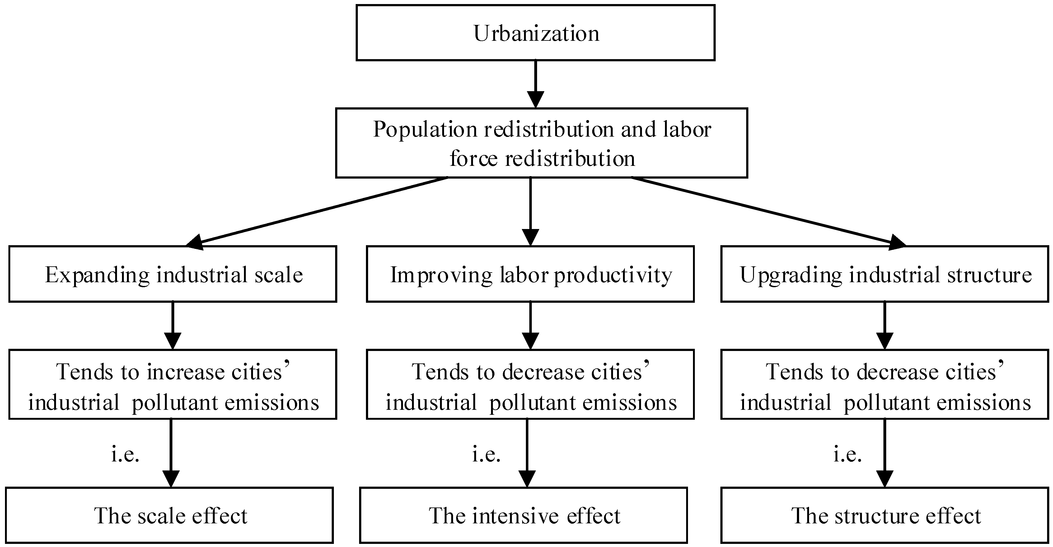
The mechanisms between urbanization and industrial pollutant emissions can be briefly and vividly described as the following process (see Figure 1): on the one hand, urbanization leads to redistribution of population and labor force between urban and rural areas. Many young, able-bodied rural people migrate to cities to work in the link of industrial production, which aggravates the total industrial pollutant emissions by expanding industrial production. On the other hand, Nakamura [27] and Fogarty and Garofalo [28] pointed out that agglomeration economic effects would be generated and enhanced during the process of urbanization, and then brought the rise of efficiency of the industrial production. Many empirical studies also stated that urban size had a clear positive relationship with the industrial production efficiency (Moomaw [29], Ciccone [30]). Consequently, we propose the core viewpoint that each unit of the industrial production’s pollutant emissions will be decreased due to urban higher productivity. Additionally, the industrial structure will also be upgraded for the reason of urban economic development and labor division, which will affect industrial pollutant emissions accordingly because different industrial sectors have different pollutant emissions intensities. For example, compared with a heavy industry-oriented economy, a service-oriented economy is always regarded as a kind of environment-friendly development mode.

In summary, the influence of urbanization on industrial pollutant emissions can be decomposed into three types of effects according to their diverse mechanisms. The scale effect indicates the expansion of industrial production and denotes a greater consumption of fossil energy and water. The intensive effect indicates the improvement of industrial technologies and denotes higher production efficiencies. The structure effect indicates the upgrading of industrial structure shifting from high-intensity pollutants emission sectors to low-intensity pollutants emission sectors. In this paper, we propose three hypotheses and we will test their validities in empirical analyses sections.

Hypothesis 1: The scale effect of urbanization tends to increase industrial pollutant emissions.

Hypothesis 2: The intensive effect of urbanization tends to decrease industrial pollutant emissions.

Hypothesis 3: The structure effect of urbanization tends to decrease industrial pollutant emissions.

We employ the Kaya Identity and the LMDI Method to establish a model to present the mechanisms between urbanization and industrial pollutant emissions in Equation (1):

$$\begin{array}{ll}pollutant& =\frac{pollutant}{output}\times \frac{output}{labor}\times \frac{labor}{population}\times population\\ & =e\times p\times q\times population\end{array}$$

(1)

where $pollutant$ denotes the total industrial pollutant emissions, $output$ denotes the total industrial production, $labor$ denotes total industrial labor force, and $population$ denotes the total population. Thus, $e=\frac{pollutant}{output}$ denotes the industrial pollutant emission intensity, $p=\frac{output}{employee}$ denotes the industrial labor productivity, and $q=\frac{labor}{population}$ denotes the employment rate.

Taking urbanization process into account, Equation (1) can be specified as:

$$\begin{array}{cc}\hfill pollutant& =\frac{pollutan{t}_u+pollutan{t}_r}{output}·\frac{outpu{t}_u+outpu{t}_r}{labor}·\frac{labo{r}_u+labo{r}_u}{population}·population\hfill \\ \hfill & =[{\alpha }_u{e}_u+(1-{\alpha }_u\left)e_r\right][{\beta }_u{p}_u+(1-{\beta }_u\left)p_r\right][{\varphi }_u{q}_u+(1-{\varphi }_u\left)q_r\right]population\hfill \end{array}$$

(2)

where subscripts $u$ and $r$ denote urban and rural areas respectively; ${\alpha }_u=\frac{outpu{t}_u}{output}$ denotes the proportion of urban industrial output in total industrial production; ${\beta }_u=\frac{labo{r}_u}{labor}$ denotes the proportion of urban industrial employees in total industrial labor force; and ${\varphi }_u=\frac{populatio{n}_u}{population}$ denotes urbanization rate.

Then taking industrial structure into account, Equation (2) can be specified as:

$$\begin{array}{ll}pollutant& =\frac{pollutan{t}_u+pollutan{t}_r}{output}·\frac{outpu{t}_u+outpu{t}_r}{labor}·\frac{labo{r}_u+labo{r}_u}{population}·population\\ & ·\frac{{\displaystyle \sum _{j=1\dots n}labo{r}_{u,j}}+{\displaystyle \sum _{j=1\dots n}labo{r}_{r,j}}}{{\displaystyle \sum _{j=1\dots n}labo{r}_j}}\\ & =[{\alpha }_u{e}_u+(1-{\alpha }_u\left)e_r\right][{\beta }_u{p}_u+(1-{\beta }_u\left)p_r\right][{\varphi }_u{q}_u+(1-{\varphi }_u\left)q_r\right]population\\ & [{\beta }_u{\displaystyle \sum _{j=1\dots n}{s}_{u,j}}+(1-{\beta }_u){\displaystyle \sum _{j=1\dots n}{s}_{r,j}}]\end{array}$$

(3)

where subscript $j$ denotes different industrial sectors and $s_{u,j}=\frac{{labor}_{u,j}}{labo{r}_u}$ denotes the proportion of employees who work in the industrial sector $j$.

Taking the logarithm for Equation (3), and then we have:

$$\begin{array}{ll}\ln pollutant& =\underset{thescaleeffect}{\underbrace{\ln \{[{\varphi }_u{q}_u+(1-{\varphi }_u)q_r]\times population\}}}+\underset{theintensiveeffect}{\underbrace{\ln [{\beta }_u{p}_u+(1-{\beta }_u)p_r]}}\\ & +\underset{thestructureeffect}{\underbrace{\ln \{[{\alpha }_u{e}_u+(1-{\alpha }_u)e_r]\times [{\beta }_u{\displaystyle \sum _{j=1,\dots ,n}{s}_{u,j}}+(1-{\beta }_u){\displaystyle \sum _{j=1,\dots ,n}{s}_{r,j}}]\}}}\end{array}$$

(4)

In Equation (4), ${\beta }_u$, ${\varphi }_u$ and ${\alpha }_u$ are variables that reflect population redistribution and labor force redistribution during the process of urbanization. According to the mechanisms analysis, we split the scale effect as $\text{ln}\left\{[{\varphi }_u{q}_u+(1-{\varphi }_u\left)q_r\right]\times population\right\}$ due to the fact that this monomial reflects the scale expansion of industrial production; we split the intensive effect as $\text{ln}[{\beta }_u{p}_u+(1-{\beta }_u\left)p_r\right]$ due to the fact that this monomial reflects the promotion of industrial productivity; we split the structure effect as $\text{ln}\left\{[{\alpha }_u{e}_u+(1-{\alpha }_u)e_r]\times [{\beta }_u{\displaystyle \sum _{j=1\dots n}{s}_{u,j}}+(1-{\beta }_u){\displaystyle \sum _{j=1\dots n}{s}_{r,j}}]\right\}$ due to the fact that this monomial reflects structure upgrading.

We argue that the decomposition is necessary and meaningful, it establishes a cornerstone in understanding the relationship between the urbanization and the industrial pollutant emissions, and effectively contributes to the relative policy making.

4. Modeling and Parameters

4.1. Modeling

According to the mechanisms analysis in Section 3, by applying the Kaya Identity and the LMDI Method, we have decomposed out the scale effect as $\text{ln}\left\{[{\varphi }_u{q}_u+(1-{\varphi }_u\left)q_r\right]\times population\right\}$, the intensive effect as $\text{ln}[{\beta }_u{p}_u+(1-{\beta }_u\left)p_r\right]$, and the structure effect as $\text{ln}\left\{[{\alpha }_u{e}_u+(1-{\alpha }_u)e_r]\times [{\beta }_u{\displaystyle \sum _{j=1\dots n}{s}_{u,j}}+(1-{\beta }_u){\displaystyle \sum _{j=1\dots n}{s}_{r,j}}]\right\}$. In order to analyze the three effects independently, we establish the traditional panel model as follows:

$$\begin{array}{ll}\text{ln} pollutant& ={\rho }_1\text{ln}scale\_effec{t}_{i,t}+{\rho }_2\text{ln}intensive\_effec{t}_{i,t}+{\rho }_3\text{ln}structure\_effec{t}_{i,t}+\pi +{\epsilon }_{i,t}\\ & ={\rho }_1\text{ln}\left\{[{\varphi }_{u,i,t}{q}_{u,i,t}+(1-{\varphi }_{u,i,t}\left)q_{r,i,t}\right]\times populatio{n}_{i,t}\right\}+{\rho }_2\text{ln}[{\beta }_{u,i,t}{p}_{u,i,t}+(1-{\beta }_{u,i,t}\left)p_{r,i,t}\right]\\ & +{\rho }_3\text{ln}\left\{[{\alpha }_{u,i,t}{e}_{u,i,t}+(1-{\alpha }_{u,i,t})e_{r,i,t}]\times [{\beta }_{u,i,t}{\displaystyle \sum _{j=1\dots n}{s}_{u,j,i,t}}+(1-{\beta }_{u,i,t}){\displaystyle \sum _{j=1\dots n}{s}_{r,j,i,t}}]\right\}+c+{\epsilon }_{i,t}\end{array}$$

(5)

where subscript $i$ denotes the cross-sections; $t$ denotes the time series; $c$ denotes the constant; ${\epsilon }_{i,t}$ denotes the random errors; and ${\rho }_1$, ${\rho }_2$ and ${\rho }_3$ are the regression coefficients of the scale effect, the intensive effect and the structure effect severally. Specifically, according to the three hypotheses in section 3, ${\rho }_1$ is expected to be positive and indicates that the scale effect will aggravate industrial pollutant emissions; ${\rho }_2$ and ${\rho }_3$ are expected to be negative and indicate that the intensive effect and the structure effect will relief the increasing trend of industrial pollutant emissions.

One of the assumptions for establishing a traditional panel model, such as Equation (5), is that different cities are completely independent from each other; that is to say, the spatial autocorrelations are non-existent or non-significant. However, this assumption has been questioned by many scholars (Arbia and Thomas-Agnan [31], LeSage [32]), who addressed that different regions’ economic developments were strongly related with each other benefiting from the development of transportation networks and communication technologies.

Therefore, the empirical results of the traditional panel model may generate biased errors due to the omission of spatial autocorrelations. To remedy the drawback, we try to apply the spatial panel model as follows:

$$\begin{array}{l}\begin{array}{ll}\text{ln} pollutan{t}_{i,t}& =\psi {\displaystyle \sum W}\text{ln}pollutan{t}_{i,t}+{\rho }_1\text{ln}scale\_effec{t}_{i,t}+{\rho }_2\text{ln}intensive\_effec{t}_{i,t}\\ & +{\rho }_3\text{ln}structure\_effec{t}_{i,t}+\pi +{\epsilon }_{i,t}\end{array}\\ {\epsilon }_{i,t}=\tau {\displaystyle \sum W}{\epsilon }_{i,t}+{\upsilon }_{i,t}\end{array}$$

(6)

where $W$ denotes the spatial weight matrix, $\psi$ is the spatial lag coefficient, and $\tau$ is the space error coefficient. Compared to the traditional panel model in Equation (5), the spatial panel model in Equation (6) is supposed to be more reasonable in two ways: firstly, it focuses on the spatial autocorrelation of the dependent variable by introducing ${\displaystyle \sum W}\text{ln}pollutan{t}_{i,t}$; and secondly, it focuses on the spatial autocorrelations of the omitted variables by extending ${\epsilon }_{i,t}$ into ${\displaystyle \sum W}{\epsilon }_{i,t}$.

Moreover, under different situations, the spatial panel model can also be subdivided into the Spatial Lag Model (SLM) and the Spatial Error Model (SEM), and which model should be chosen can be assessed by the Lagrange Multipliers (LM) and the robustness tests (Lee and Yu [33], Elhorst [34]). Specifically, if the Lagrange Multiplier of SLM (LM_lag) is more significant than that of SEM (LM_error), and the robustness of SLM (robustness_lag) passes significance testing while the robustness of SEM (robustness_error) does not, then the Spatial Lag Model will be more suitable. Otherwise, the Spatial Error Model will be more suitable.

4.2. Parameters

In this paper, the spatial panel model is established on the basis of the data from 282 prefecture-level cities in China from 2003 to 2014. The main data are extracted from the China City Statistical Yearbook. In addition, the following is a brief introduction to the parameters.

In terms of the dependent variables, industrial pollutant emissions ($pollutant$) are measured by the volume of industrial wastewater discharge ($pollutant\_water$), the volume of industrial sulfur dioxide emissions ($pollutant\_sulphur$) and the volume of industrial soot (dust) emissions ($pollutant\_soot$), respectively.

In terms of the independent variables, employment rates ($q_u,q_r$) are measured by the ratio of industrial employees to the total population; industrial labor productivities ($p_{u,j},p_{r,j}$) are measured by industrial output per unit of labor; pollutant emissions intensities ($e_{u,j},e_{r,j}$) are measured by the ratios of each sector’s pollutant emissions to their industrial output; industrial structures ($s_{u,j},s_{r,j}$) are measured by the proportions of employees in each industrial sector; and the distributions of population (${\varphi }_u$), industrial employee (${\beta }_u$) and industrial output (${\alpha }_u$) between urban and rural areas are measured by their proportions in cities.

The spatial weight matrix ($W$) is measured by the reciprocal of the geographic distances between different cities.

5. Empirical Analysis

5.1. Description of the Relationship between Urbanization and Industrial Pollutants Emissions

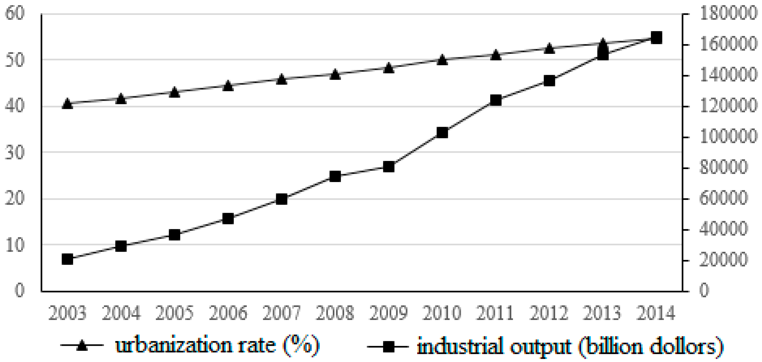
Figure 2 reports the trends of China’s urbanization rate and the industrial output from 2003 to 2014. It exhibits that China’s urbanization rate rose steadily from 40.53% in 2003 to 54.77% in 2014. During the same period of time, China’s industrial output also showed a gradual upward trend. Figure 2 supports the view that China’s urbanization expands the industrial production, which is referred as the demographic dividend by many economic scholars (Peng [35], Golley and Tyers [36]).

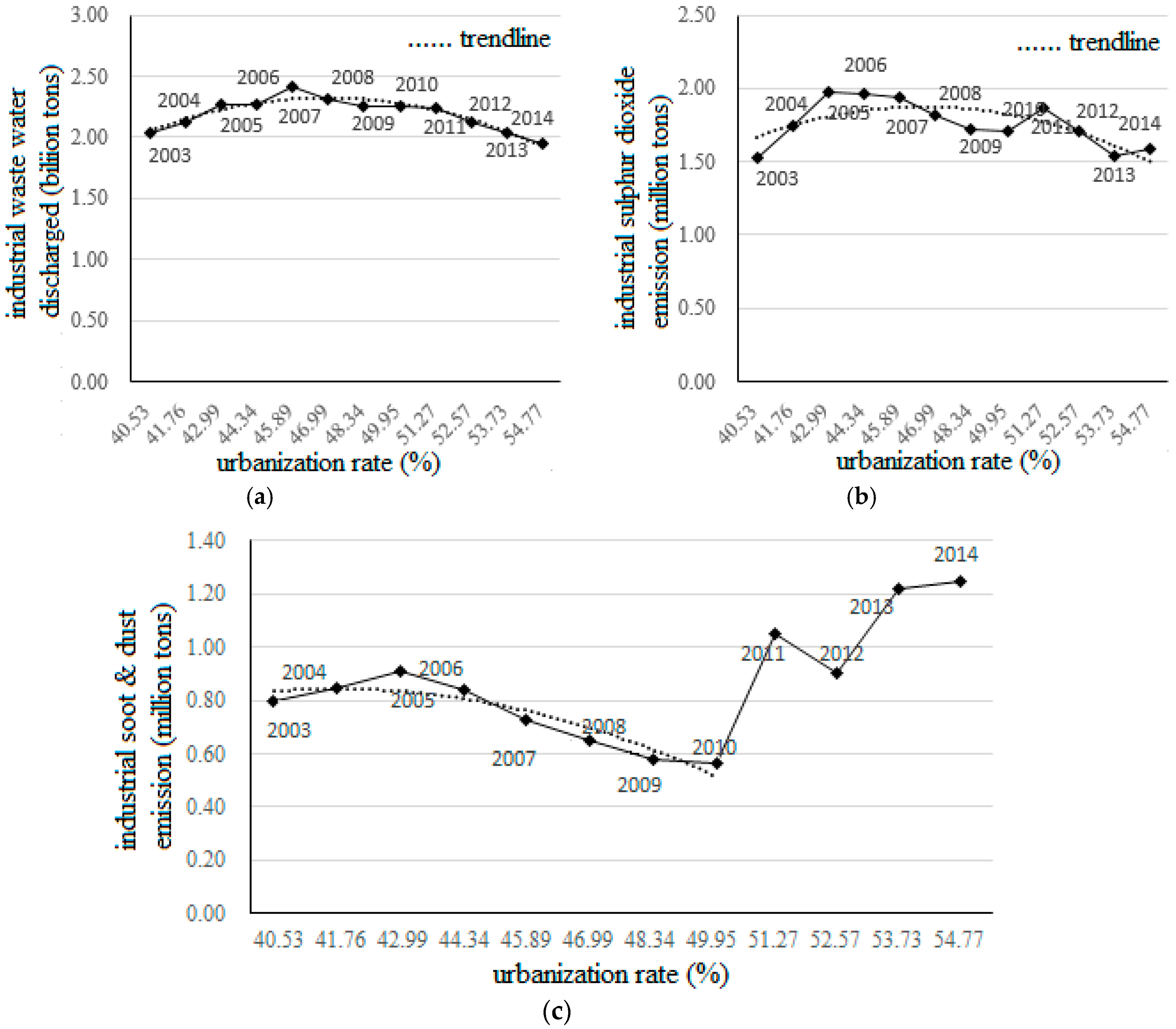
Figure 3a–c report the relationships between China’s urbanization rate and the three types of industrial pollutant emissions from 2003 to 2014. It has been found that with the steady rise of China’s urbanization rate, the volume of the industrial wastewater discharge increased continually and reached its peak in 2007. After that, the volume of industrial wastewater discharge showed a downward trend. The curves of the volume of industrial sulfur dioxide emissions and industrial soot (dust) emissions of China also fitted reverse U-shapes, especially from the year 2003 to the year 2010.

In conclusion, the relationships between China’s urbanization rate and the three types of industrial pollutant emissions indicate that at the beginning stage of China’s urbanization, the three types of industrial pollutant emissions are positive related with the increase of the urbanization rate. However, with further development in China’s urbanization, the three types of industrial pollutant emissions are negative related with the increase of the urbanization rate. Therefore, we argue that the relationship between China’s urbanization and the industrial pollutant emissions is not constant.

5.2. Test of the Spatial Autocorrelations of Industrial Pollutant Emissions

In this paper, we apply the Moran’s Index to test the spatial autocorrelations of the industrial pollutant emissions among China’s cities. The Moran’s Index can be calculated in Equation (7).

$$Moran’sI=\frac{{\displaystyle \sum _{c2}{\displaystyle \sum _{c1}W(pollutan{t}_{c1}-\stackrel{-}{pollutant})(pollutan{t}_{c2}-\stackrel{-}{pollutant})}}}{S^2{\displaystyle \sum _{c2}{\displaystyle \sum _{c1}W}}}$$

(7)

where $c1$ and $c2$ denote different cities, $\stackrel{-}{pollutant}$ denotes the average industrial pollutant emissions of all the cities, $W$ denotes the spatial weight matrix, $S^2=\frac{1}{n}{\displaystyle \sum _{c1}（pollutan{t}_{c1}-\stackrel{-}{pollutant}）}$ and $n$ denotes the number of cities.

Table 1. The Moran’s Indexes of the industrial pollutant emissions among China’s cities.

	2003	2004	2005	2006	2007	2008
pollutant_water	0.050 *** (8.054)	0.057 *** (9.136)	0.064 *** (10.183)	0.076 *** (12.019)	0.078 *** (12.349)	0.075 *** (11.866)
pollutant_sulfur	0.048 *** (7.851)	0.045 *** (7.328)	0.052 *** (8.416)	0.053 *** (8.473)	0.036 *** (6.049)	0.040 *** (6.639)
pollutant_soot	0.085 *** (13.390)	0.080 *** (12.593)	0.083 *** (13.068)	0.086 *** (13.563)	0.071 *** (11.303)	0.066 *** (10.500)
	2009	2010	2011	2012	2013	2014
pollutant_water	0.080 *** (12.663)	0.082 *** (12.967)	0.087 *** (13.646)	0.085 *** (13.293)	0.084 *** (13.152)	0.084 *** (13.272)
pollutant_sulfur	0.035 *** (5.877)	0.031 *** (5.390)	0.052 *** (8.507)	0.058 *** (9.469)	0.083 *** (13.229)	0.057 *** (9.620)
pollutant_soot	0.063 *** (10.121)	0.053 *** (8.637)	0.094 *** (14.795)	0.087 *** (13.737)	0.086 *** (13.488)	0.085 *** (13.297)

Notes: The figures in () are Z statistics; ***, ** and * denote the level of significance at 1%, 5% and 10%, respectively.

reports the Moran’s Indexes of the three types of industrial pollutant emissions among China’s cities from 2003 to 2014. We can conclude from Table 1 that all the Moran’s Indexes are significant and positive, which indicates that there are significant spatial autocorrelations of the industrial pollutant emissions among different cities.

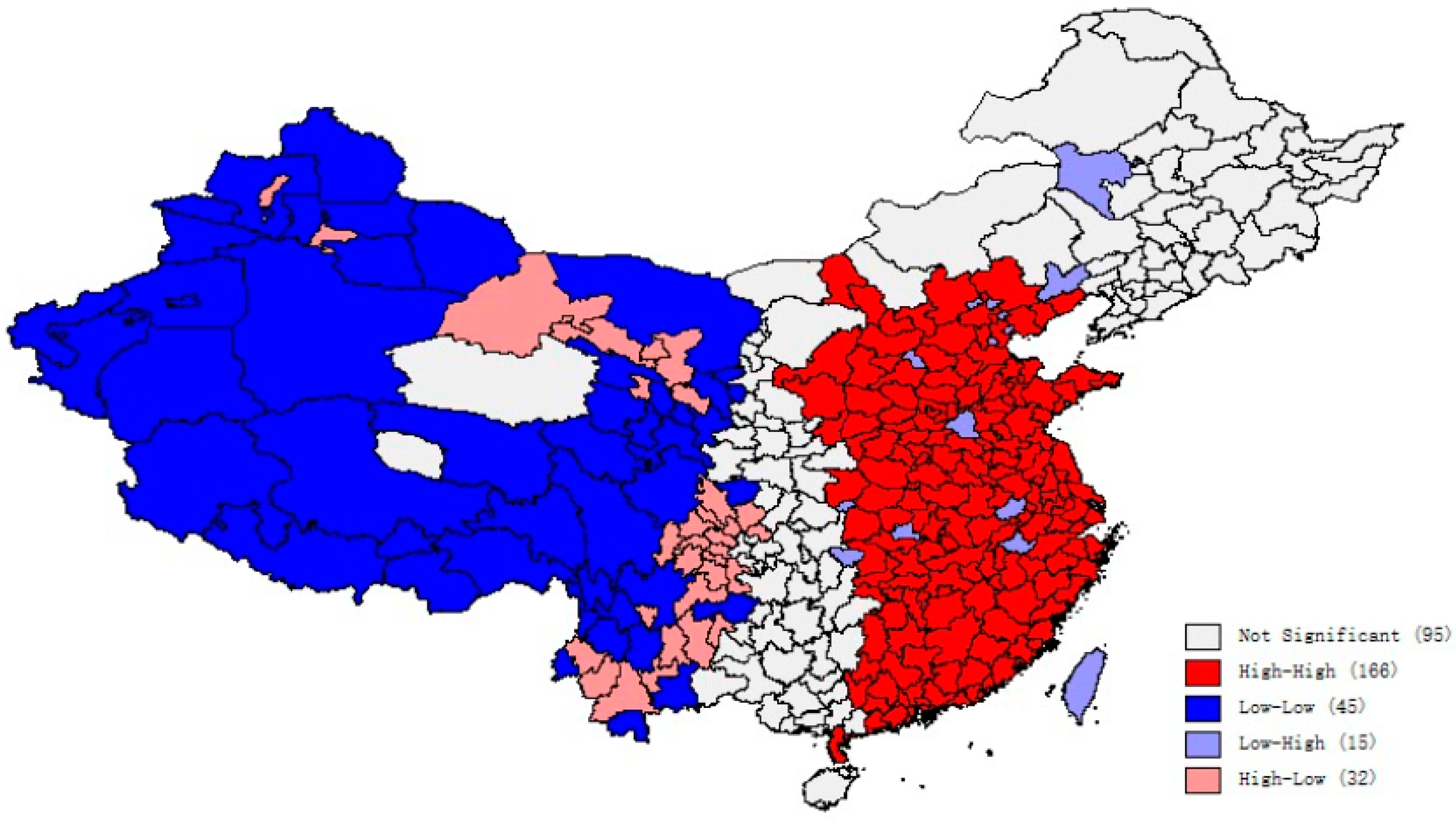
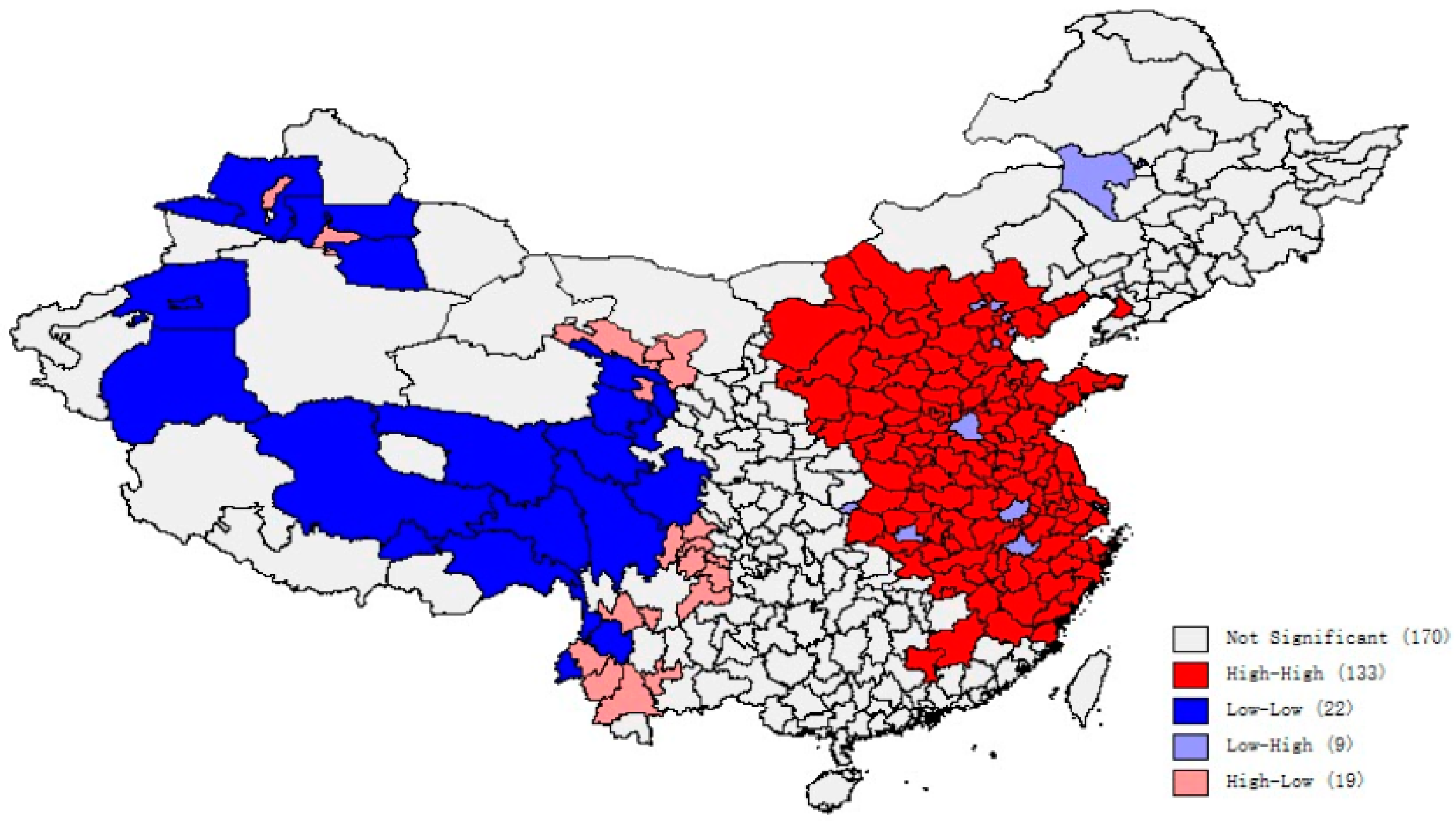
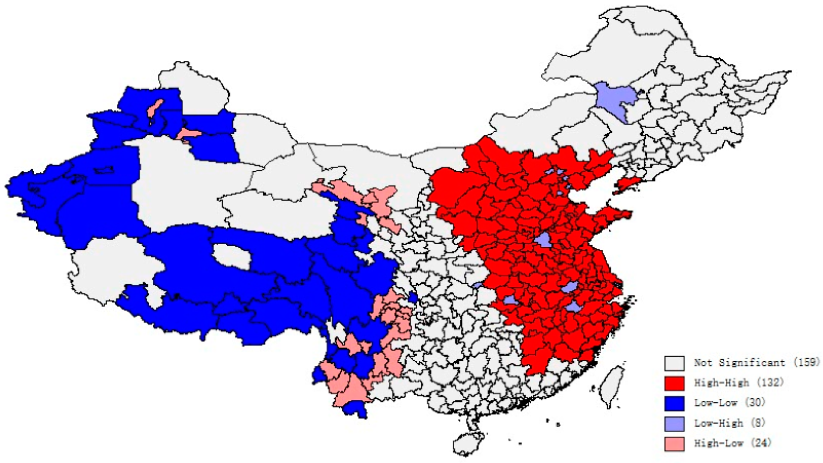
Figure 4, Figure 5 and Figure 6 show the cluster maps of three types of industrial pollutant emissions of China’s cities in 2014, respectively. It can be found that the High-High clusters of the industrial wastewater discharge are concentrated in most of eastern cities and some of central cities in China. The High-High clusters of the industrial sulfur dioxide emissions and the soot (dust) emissions are concentrated in China’s Beijing-Tianjin-Hebei region and the Yangtze River Delta. Most cities in western China present the state of Low-Low clusters or do not pass the statistical significance testing.

The most important conclusion we can draw from the above testing is that there are significant spatial autocorrelations of industrial pollutant emissions among different cities, and therefore it is more reasonable to apply the spatial panel model in this paper.

5.3. Regression Result Analyses

5.3.1. Analyses of the Scale Effect, the Intensive Effect and the Structure Effect

Table 2. The regression results of the scale effect, the intensive effect and the structure effect.

Model	OLS		SLM		SEM
	Non-FE	FE	Non-FE	FE	Non-FE	FE
dependent variables	pollutant_water
scale effect (ρ1)	0.532 *** (25.433)	0.547 *** (25.513)	0.511 *** (24.861)	0.499 *** (24.347)	0.495 *** (24.888)	0.492 *** (24.666)
intensive effect (ρ2)	−0.114 *** (−5.692)	−0.140 *** (−5.917)	−0.087 *** (−4.435)	−0.059 *** (−3.390)	−0.074 *** (−5.050)	−0.068 *** (−4.958)
structure effect (ρ3)	0.585 *** (12.814)	0.605 *** (12.914)	0.544 *** (12.098)	0.515 *** (11.596)	0.543 *** (12.482)	0.534 *** (12.292)
LM spatial lag	373.112 ***	445.778 ***
Robust LM spatial lag	97.479 ***	34.532 ***
LM spatial error	278.750 ***	434.746 ***
Robust LM spatial error	3.117 *	23.500 ***
Adj-R2	0.301	0.304	0.332	0.323	0.330	0.322
Log-likelihood	−4.428 × 103	−4.416 × 103	−1.451 × 103	−4.380 × 103	−4.361 × 103	−4.382 × 103
dependent variables	pollutant_sulfur
scale effect (ρ1)	0.361 *** (15.289)	0.366 *** (15.223)	0.359 *** (15.183)	0.360 *** (15.283)	0.360 *** (15.279)	0.356 *** (15.128)
intensive effect (ρ2)	−0.054 ** (−2.399)	−0.049 * (−1.847)	−0.053 ** (−2.334)	−0.062 *** (−3.079)	−0.054 ** (−2.413)	−0.058 *** (−2.938)
structure effect (ρ3)	0.779 *** (15.118)	0.771 *** (14.679)	0.777 *** (15.030)	0.776 *** (15.240)	0.779 *** (15.147)	0.771 *** (15.172)
LM spatial lag	9.492 **	195.330 ***
Robust LM spatial lag	48.477 ***	4.176 **
LM spatial error	0.378	205.698 ***
Robust LM spatial error	39.363 ***	14.544 ***
Adj-R2	0.212	0.218	0.213	0.201	0.212	0.199
Log-likelihood	−4.836 × 103	−4.803 × 103	−4.835 × 10 3	−4.867 × 103	−4.836 × 103	−4.864 × 103
dependent variables	pollutant_soot
scale effect ( ρ1)	0.343 *** (14.153)	0.367 *** (15.045)	0.341 *** (14.122)	0.362 *** (15.042)	0.341 *** (14.110)	0.356 *** (14.791)
intensive effect (ρ2)	−0.084 *** (−3.643)	−0.170 *** (−6.326)	−0.083 *** (−3.578)	−0.076 *** (−3.709)	−0.080 *** (−3.507)	−0.053 *** (−2.648)
structure effect (ρ3)	0.485 *** (9.177)	0.556 *** (10.443)	0.483 *** (9.138)	0.452 *** (8.683)	0.481 *** (9.119)	0.424 *** (8.148)
LM spatial lag	1.811	719.109***
Robust LM spatial lag	5.722 **	74.425 ***
LM spatial error	0.518	644.690 ***
Robust LM spatial error	4.430 **	0.006
Adj-R2	0.130	0.132	0.130	0.122	0.130	0.118
Log-likelihood	−4.921 × 103	−4.851 × 103	−4.921 × 103	−4.949 × 103	−4.921 × 103	−4.944 × 103

Notes: The figures in () are Z statistics; ***, ** and * denote the level of significance at 1%, 5% and 10%, respectively.

reports the regression results of the scale effect, the intensive effect and the structure effect of China’s urbanization impacts on the industrial wastewater discharge, the sulfur dioxide emissions, and the soot (dust) emissions.

We list the regression results of three models: the OLS is the regression results by applying the traditional panel model and the SLM and the SEM are the regression results by applying the Spatial Lag Model and the Spatial Error Model in the proper order. The Non-FE denotes regression results without fixed effects, while FE denotes regression results with fixed effects. Following the rules in Section 4.1, we finally choose the Spatial Lag Model with fixed effect as the optimal model, and regard other models as control groups.

We can infer from Table 2 that the regression coefficients $\rho 1$, $\rho 2$ and $\rho 3$ have passed the significance testing, and $\rho 1$, $\rho 3$ are positive in each model, while $\rho 2$ are always negative. As $\rho 1$, $\rho 2$ and $\rho 3$ reflect the impacts of the scale effect, the intensive effect and the structure effect of China’s urbanization on the industrial pollutant emissions, we can draw the conclusion that the scale effect and the structure effect tend to aggravate the industrial wastewater discharge, the sulfur dioxide emissions and the soot (dust) emissions in China’s cities; however, the intensive effect results in decreasing the industrial pollutant emissions in China’s cities.

The signs of the scale effect and the intensive effect are in line with our expectations, but the sign of the structure effect is beyond our expectation. That is to say, our results accept Hypothesis 1 and Hypothesis 2 but clearly reject Hypothesis 3. Specifically, the population redistribution and labor force redistribution during China’s urbanization enhance the expansion of the industrial production and generate increasing industrial pollutant emissions. The improvement of the industrial labor productivity in China’s cities decreases each unit of the industrial production’s pollutant emissions and generates an ameliorative impact on the industrial pollutant emissions. However, the changes of the industrial structure in China’s cities aggravate the industrial pollutant emissions rather than decelerate them. Accordingly, we conclude that China appears to be following a path similar to that trodden by some earlier industrialized countries, and the development of its high-tech and service industries shows slow growth tendencies.

5.3.2. Analyses of the Spatial Spillover Effect

Table 3. The regression results of the spatial spillover effect.

Model	SLM		SEM
	Non-FE	FE	Non-FE	FE
dependent variables	pollutant_water
spatial lag coefficient (ψ)	−0.766 *** (−3.968)	0.673 *** (−3.579)
spatial error coefficient (τ)			−0.990 *** (−3.719)	−0.990 *** (−3.719)
dependent variables	pollutant_sulfur
spatial lag coefficient (ψ)	−0.073 (−0.423)	0.107 (0.712)
spatial error coefficient (τ)			−0.030 (−0.161)	−0.026 (−0.140)
dependent variables	pollutant_soot
spatial lag coefficient (ψ)	−0.021 (−0.119)	0.150 (0.999)
spatial error coefficient (τ)			−0.028 (−0.150)	−0.069 (−0.359)

Notes: The figures in () are Z statistics; ***, ** and * denote the level of significance at 1%, 5% and 10%, respectively.

reports the spatial lag coefficient (ψ) and the spatial error coefficient (τ). By analyzing these coefficients, we can shed light on the spatial spillover effect of China’s urbanization on the industrial pollutant emissions.

In terms of the industrial wastewater discharge in China’s cities, both the spatial lag coefficient (ψ) and the spatial error coefficient (τ) are significant and negative; however, in terms of the industrial sulfur dioxide emissions and the industrial soot (dust) emissions in China’s cities, neither of the spatial coefficients passes the statistical significance testing. That is to say, the spatial spillover of the industrial pollutant emissions from other cities does not aggravate the local city’s industrial pollutant emissions. This result is beyond our expectation, moreover, it contradicts the conclusion, which we draw from Section 5.3.1: there are significant spatial autocorrelations of the industrial pollutant emissions among different cities, but the spatial spillover effect is non-existent or non-significant.

We come up with an explanation to the contradiction that there are vast rural areas around China’s cities, such vast rural areas serve as sponge belts and absorb the spatial spillover of the industrial pollutant emissions from cities, so the spatial spillover effect is non-existent or non-significant. However, from another point of view, cross-regional economic relationships are shown in many forms, such as population flows, industrial associations, and resource exchanges, these cross-regional activities induce significant spatial autocorrelations among different cities, but the industrial pollutant emissions themselves in different cities fail to affect each other.

6. Discussion and Conclusions

In this paper, we first decompose the influence of urbanization impacts on the industrial pollutant emissions into the scale effect, the intensive effect and the structure effect by using the Kaya Identity and the LMDI Method; second, we perform an empirical study of the three effects by applying the spatial panel model on the basis of the data from 282 prefecture-level cities in China from 2003 to 2014. Our results indicate that (1) there are significant reverse U-shapes between China’s urbanization rate and the volume of industrial wastewater discharge, sulfur dioxide emissions and soot (dust) emissions; (2) the relationship between China’s urbanization and the industrial pollutant emissions depends on the scale effect, the intensive effect and the structure effect jointly. Specifically, the scale effect and the structure effect tend to aggravate the industrial wastewater discharge, the sulfur dioxide emissions and the soot (dust) emissions in China’s cities, while the intensive effect results in decreasing the three types of the industrial pollutant emissions. The signs of the scale effect and the intensive effect are in line with our expectations, but the sign of the structure effect is beyond our expectation, we conclude that China appears to be following a path similar to that trodden by some earlier industrialized countries, and the development of its high-tech and service industries shows slow growth tendencies; (3) there are significant spatial autocorrelations of the industrial pollutant emissions among China’s cities, but the spatial spillover effect is non-existent or non-significant, we attempt to explain this contradiction due to the fact that the vast rural areas around China’s cities serve as sponge belts and absorb the spatial spillover of the industrial pollutant emissions from cities.

Based on the above conclusions, we argue that even though urbanization has correlations with industrial pollutant emissions, their definite relationship should be considered cautiously, because it depends on the combined influence of the scale effect, the intensive effect and the structure effect. China is in a phase of rapid urbanization, and tremendous efforts have been made in relieving the industrial pollutant emissions, but our research suggests that the lock-in of the heavily polluting industries has challenged our attempt to reduce the environmental pollution. Fortunately, the vast rural areas around China’s cities have absorbed and eased the spatial spillover of the industrial pollutant emissions from cities. However, with the spreading of industrialization to China’s countryside, the rural areas are facing a growing threat of industrial pollution.

References

Johnson, T.M.; Liu, F.; Newfarmer, R. The World Bank. In Clear Water, Blue Skies: China's Environment in the New Century; World Bank Publications: Washington, DC, USA, 1997. [Google Scholar]
The World Bank. Cost of Pollution in China: Economic Estimates of Physical Damages; World Bank Publications: Washington, DC, USA, 2007. [Google Scholar]
Easterlin, R.A.; Morgan, R.; Switek, M.; Wang, F. China’s life satisfaction, 1990–2010. Available online: http://www.pnas.org/content/109/25/9775.short (accessed on 9 August 2016).
Vennemo, H.; Aunan, K.; Lindhjem, H.; Seip, H.M. Environmental pollution in China: status and trends. Rev. Environ. Econ. Policy2009, 3, 209–230. [Google Scholar]
Tolley, G.S. The welfare economics of city bigness. J. Urban Econ.1974, 1, 324–345. [Google Scholar] [CrossRef]
Glaeser, E.L. Are cities dying? J. Econ. Perspect.1998, 12, 139–160. [Google Scholar] [CrossRef]
Wan, G.; Wang, C. Unprecedented Urbanization in Asia and Its Impacts on the Environment. Aust. Econ. Rev.2014, 47, 378–385. [Google Scholar] [CrossRef]
Grossman, G.M.; Krueger, A.B. Environmental impacts of a North American free trade agreement. Available online: http://www.nber.org/papers/w3914.pdf (accessed on 8 August 2016).
Grossman, G.M.; Krueger, A.B. Economic growth and the environment. Available online: http://www.nber.org/papers/w4634.pdf (assessed on 8 August 2016).
Lindmark, M. An EKC-pattern in historical perspective: carbon dioxide emissions, technology, fuel prices and growth in Sweden 1870–1997. Ecol. Econ.2002, 42, 333–347. [Google Scholar] [CrossRef]
Nasir, M.; Rehman, F.U. Environmental Kuznets curve for carbon emissions in Pakistan: An empirical investigation. Energy Policy2011, 39, 1857–1864. [Google Scholar] [CrossRef]
Esteve, V.; Tamarit, C. Threshold cointegration and nonlinear adjustment between CO2 and income: The environmental Kuznets curve in Spain, 1857–2007. Energy Econ.2012, 34, 2148–2156. [Google Scholar] [CrossRef]
Jalil, A.; Mahmud, S.F. Environment Kuznets curve for CO2 emissions: a cointegration analysis for China. Energy Policy2009, 37, 5167–5172. [Google Scholar] [CrossRef]
Li, T.; Wang, Y.; Zhao, D. Environmental Kuznets Curve in China: New evidence from dynamic panel analysis. Energy Policy2016, 91, 138–147. [Google Scholar] [CrossRef]
Stern, D.I.; Common, M.S. Is there an environmental Kuznets curve for sulfur? J. Environ. Econ. Manag.2001, 41, 162–178. [Google Scholar] [CrossRef]
York, R.; Rosa, E.A.; Dietz, T. STIRPAT, IPAT and ImPACT: Analytic tools for unpacking the driving forces of environmental impacts. Ecol. Econ.2003, 46, 351–365. [Google Scholar] [CrossRef]
Kwon, T.H. Decomposition of factors determining the trend of CO2 emissions from car travel in Great Britain (1970–2000). Ecol. Econ.2005, 53, 261–275. [Google Scholar] [CrossRef]
Dasgupta, S.; Laplante, B.; Wang, H.; Wheeler, D. Confronting the environmental Kuznets curve. J. Econ. Perspect.2002, 16, 147–168. [Google Scholar] [CrossRef]
Panayotou, T. Economic growth and the environment. Economic Survey of Europe.2003, 2, 45–72. [Google Scholar]
Kanada, M.; Dong, L.; Fujita, T.; Fujii, M.; Inoue, T.; Hirano, Y.; Togawa, T.; Geng, Y. Regional disparity and cost-effective SO2 pollution control in China: a case study in 5 mega-cities. Energy policy2013, 61, 1322–1331. [Google Scholar] [CrossRef]
Qin, H.; Su, Q.; Khu, S.T.; Tang, N. Water Quality changes during rapid urbanization in the Shenzhen river catchment: An integrated view of socio-economic and infrastructure development. Sustain2014, 6, 7433–7451. [Google Scholar] [CrossRef]
Dong, H.; Dai, H.; Dong, L.; Fujita, T.; Geng, Y.; Klimont, Z.; Inoue, T.; Bunya, S.; Fujii, M.; Masui, T. Pursuing air pollutant co-benefits of CO2 mitigation in China: A provincial leveled analysis. Appl. Energy2015, 144, 165–174. [Google Scholar] [CrossRef]
Tao, Y.; Li, F.; Crittenden, J.C.; Lu, Z.; Sun, X. Environmental Impacts of China’s Urbanization from 2000 to 2010 and Management Implications. Environ. Manag.2016, 57, 498–507. [Google Scholar] [CrossRef] [PubMed]
Nakamura, R. Agglomeration economies in urban manufacturing industries: a case of Japanese cities. J. Urban Econ.1985, 17, 108–124. [Google Scholar] [CrossRef]
Fogarty, M.S.; Garofalo, G.A. Urban spatial structure and productivity growth in the manufacturing sector of cities. J. Urban Econ.1988, 23, 60–70. [Google Scholar] [CrossRef]
Moomaw, R.L. Productivity and city size: a critique of the evidence. Q. J. Econ.1981, 96, 675–688. [Google Scholar] [CrossRef]
Ciccone, A. Agglomeration effects in Europe. Eur. Econ. Rev.2002, 46, 213–227. [Google Scholar] [CrossRef]
Arbia, G.; Thomas-Agnan, C. Introduction: Advances in Cross-Sectional and Panel Data Spatial Econometric Modeling. Geogr. Anal.2014, 46, 101–103. [Google Scholar] [CrossRef]
LeSage, J.P. Software for Bayesian cross section and panel spatial model comparison. J. Geogr. Syst.2015, 17, 297–310. [Google Scholar] [CrossRef]
Lee, L.; Yu, J. Estimation of spatial autoregressive panel data models with fixed effects. J. Econ.2010, 154, 165–185. [Google Scholar] [CrossRef]
Elhorst, J.P. Specification and estimation of spatial panel data models. Int. Reg. Sci. Rev.2003, 26, 244–268. [Google Scholar] [CrossRef]
Peng, X. Understanding China's demographic dividends and labor issue. J. Policy Anal. Manag.2013, 32, 408–410. [Google Scholar] [CrossRef]
Golley, J.; Tyers, R. Demographic Dividends, Dependencies, and Economic Growth in China and India. Asian Econ. Pap.2012, 11, 1–26. [Google Scholar] [CrossRef]