Article

Ecological Security and Ecosystem Services in Response to Land Use Change in the Coastal Area of Jiangsu, China

1
School of Geographic and Oceanographic Sciences, Nanjing University, Nanjing 210023, China
2
The Key Laboratory of the Coastal Zone Exploitation and Protection, Ministry of Land and Resources, Nanjing 210023, China
3
School of Geography, Geomatics and Planning, Jiangsu Normal University, Xuzhou 221116, China
*
Author to whom correspondence should be addressed.
Sustainability 2016, 8(8), 816; https://0-doi-org.brum.beds.ac.uk/10.3390/su8080816
Submission received: 18 June 2016 / Revised: 10 August 2016 / Accepted: 11 August 2016 / Published: 19 August 2016

Abstract

:
Urbanization, and the resulting land use/cover change, is a primary cause of the degradation of coastal wetland ecosystems. Reclamation projects are seen as a way to strike a balance between socioeconomic development and maintenance of coastal ecosystems. Our aim was to understand the ecological changes to Jiangsu’s coastal wetland resulting from land use change since 1977 by using remote sensing and spatial analyses. The results indicate that: (1) The area of artificial land use expanded while natural land use was reduced, which emphasized an increase in production-orientated land uses at the expense of ecologically important wetlands; (2) It took 34 years for landscape ecological security and 39 years for ecosystem services to regain equilibrium. The coastal reclamation area would recover ecological equilibrium only after a minimum of 30 years; (3) The total ecosystem service value decreased significantly from $2.98 billion per year to $2.31 billion per year from 1977 to 2014. Food production was the only one ecosystem service function that consistently increased, mainly because of government policy; (4) The relationship between landscape ecological security and ecosystem services is complicated, mainly because of the scale effect of landscape ecology. Spatial analysis of changing gravity centers showed that landscape ecological security and ecosystem service quality became better in the north than the south over the study period.

Graphical Abstract

1. Introduction

Urbanization is a major cause of the loss of coastal wetlands [1], and can directly transform landscapes and affect biodiversity, ecosystem productivity, and biogeochemical cycles [2,3,4,5,6]. Furthermore, it can also indirectly influence ecosystems across various scales by altering abiotic environmental conditions, including climate, and soil properties, and biotic components, such as introduced exotic species [7,8,9,10]. Land use/cover change (LUCC), partly driving by rapid urban growth [11], has occurred at an unprecedented rate in recent human history and is having a marked effect on the natural environment, including the quality of water [12], soil [13] and air resources, ecosystem services [14,15,16] and climate [17], at regional and global scale. As urbanization requires more infrastructure for housing, businesses, and transport networks, the demand for such development in coastal region is often met through exploiting natural lands (e.g., tidal flats, salt marshes, water bodies, and open spaces), which ultimately considerably reduces the ecological land of that region.
Apart from urbanization, coastal wetland is, per se, a vulnerable ecosystem with a dynamic interaction between the ocean and land. The vulnerability brings it reduced habitat complexity, decreasing biodiversity, and declining productivity, as well as high risks of storm surges, severe waves, and tsunamis. Furthermore, the Intergovernmental Panel on Climate Change (IPCC) has reported that global climate change has a serious effect on the natural environment and human society in coastal zones [18,19,20]. Additionally, the global change currently observed is deemed to accelerate coastal erosion and increase the frequency and intensity of extreme weather events [21]. For example, 15% of the 84-km Tuticorin coastal stretch is deemed high risk, and coastal erosion, slope and relative sea level rise are the major factors affecting its coastal vulnerability in Tuticorin [22]; 20.1% (57.9 km) of the total coastline in the Ganges delta is very highly vulnerable [23]; and 31% (365 km) of the Red Sea coast in Egypt is classified as the most severely sensitive [24]. Coastal place vulnerability is highly differentiated and influenced by a range of social, economic, and physical indicators [25]. Thus, coastal wetlands with multi-hazard threats attract greater attention worldwide.
The ecological restoration of coastal wetland has been under way. The International Geosphere-Biosphere Programme (IGBP, 1986–2015) and the International Human Dimensions Programme on Global Environmental Change (IHDP, 1996–2014) launched an international research project in 1993—Future Earth Coasts (formerly the Land-Oceans in the Coastal Zone, LOICZ), the vision of which is to support sustainability and adaptation to global change in the coastal zones. Natural coastal wetlands play a vital role in sustainable development of China [26]. However, with the spread of urbanization, reclamation projects have become an important measure to solve the contradiction between the rapid expansion of economic development and the shortage of resources. Reclamation projects appear worldwide, such as the Zuiderzee project in the Netherlands [27], the Isahaya Bay project in Japan [28], and the Saemangeum reclamation project in Korea [29]. In recent decades, sea enclosing and land reclamation have also become important ways for China to accommodate the increasing need for living space and development, seen for example, in Jiangsu, Shanghai, Zhejiang and Fujian Provinces [30]. This is directly reflected by LUCC and has resulted in the building of many seawalls. The seawalls, called the new “Great Wall”, cover 60% of the total length of coastline of mainland China, which have caused a significant decrease in biodiversity and ecosystem services, and will threaten regional ecological security and sustainablility [31]. Therefore, researchers worldwide are focusing on methods to guarantee the health and sustainable development of coastal wetland ecosystem.
In China, the coastal zone is a densely populated area within a fragile ecological system. The Outline of Jiangsu Coastal Reclamation Development Plan (2010–2020) was passed by the State Council of China in 2009, and predicted that the reclamation area in the Jiangsu coastal wetland would increase to 0.18 million ha by 2020 [32]. This suggests that the wetland is and will suffer from increasingly serious degradation. Chinese scholars have extensively studied the land use and environmental change of the coastal wetlands in Jiangsu Province over the last couple of decades, specifically including deposition, soil quality, spatial pattern, invasive species, biodiversity, and ecological security [33,34,35,36,37]. Because the pace of China’s coastal reclamation has been steadily increasing, the deteriorating trend of its detrimental influences on the coastal wetland ecosystems and their services has not been turned around [30]. It is necessary to quantify the chronological influence on coastal wetland ecosystem to provide a reference for policymakers.
Landscape ecology is often considered “a holistic and transdisciplinary science of landscape study, appraisal, history, planning and management, conservation, and restoration” [38,39]. A variety of landscape metrics have been built and used to quantify spatial patterns of land cover patches, classes, or entire landscape mosaics of a geographic area [40,41]. A large amount of recent studies have quantitatively evaluated the structures and patterns of landscapes [42,43,44,45,46] and ecological security [47,48,49] using land use/cover data with a range of landscape metrics or indices. Therefore, comprehensive knowledge about the chronology and process of land use change and its effect on the ecosystem integrity and health plays an important role in curbing human impacts on the environment [50], in ecological restoration, and in formulating appropriate land use planning [51]. Landscape ecology and landscape metrics are also helpful to enrich current knowledge.
In this paper, we selected the main body of the Jiangsu coastal wetland—the Jiangsu central coastal zone—as our study area. We explored ecological environmental quality (e.g., landscape ecological security and ecosystem service) from 1977 to 2014 with the aim of guaranteeing the future sustainability of these coastal wetlands under reclamation activities (reflected by land use and land cover). 
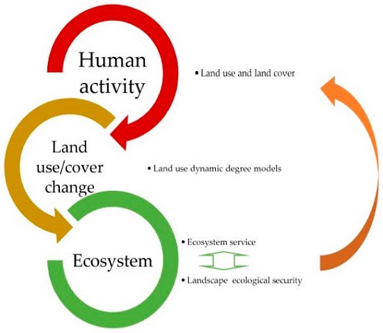
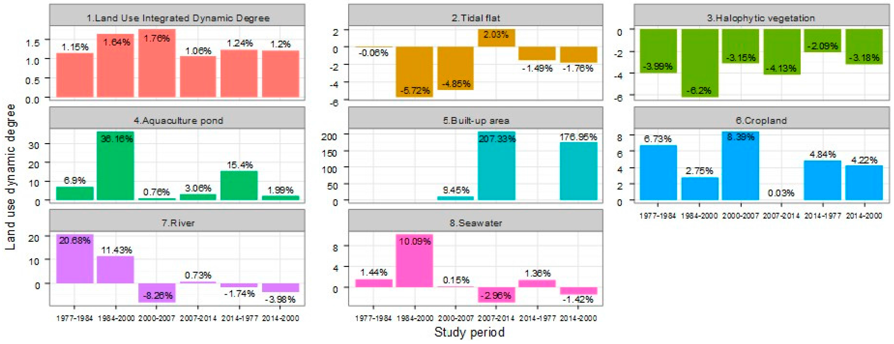
Figure 1 demonstrates the framework of this study. Here, the varying features of landscape ecological security and ecosystem services values were analyzed to get a comprehensive picture of the environmental quality of the coastal reclamation area. The objectives of this study were to: (1) briefly describe land use change and its dynamic degree; (2) analyze landscape ecological security and the relationship with the reclamation year; (3) estimate variations in ecosystem services values in response to land use change and their relationship with the reclamation year; and (4) explore the spatially changing characteristics of landscape ecological security and ecosystem service values and the correlation between them.

2. Data and Methodology

2.1. Study Area

The coastal wetland of Jiangsu Province, China, ranging from the mouth of the Xiuzhen River in the north to the northern branch of the Yangtze River in the south, covers one fourth (10,623 km2) of the total coastal area in China [52] and is considered Asia’s largest prograding mudflat [53]. The mainland coastline is about 954 km long, 93% of which is silty mud [35]. Ninety percent of the entire coastline along the Jiangsu coast is tidal flat [54]. Research shows that the coastal tidal flat is currently expanding seaward at a rate of ±20 cm per year [55,56,57]. The study area, which is about 0.38 million ha, including part of the Yellow Sea and South Yellow Sea Radial Sand Ridges, is located in the central part of the coastal zone of Jiangsu Province (Figure 2). Dafeng Père David’s Deer National Nature Reserve and Yancheng Rare Birds National Nature Reserve are located here because of the region’s abundant tidal flat resources. The study area contains four administrative units: Sheyang, Dafeng, Dongtai and Rudong. The climate is classified as subtropical monsoon with an average annual temperatures of 14 °C, annual precipitation of 1000 mm and annual sunshine of 2238.9 h [55].

2.2. Data Collection

The land use and land cover information of the study area was mainly calculated from remote sensing images (Table 1) and the accuracy of classification was checked through field work. The dates of the images were in the growth period of plants to help acquire land cover information. Geometric rectification and spatial registration technology with ENVI 5.0 (Exelis, Boulder, CO, USA) was carried out to keep spatial consistency across different images and ground objects. Then, we clipped the images to the same boundary as administrative demarcation using ArcGIS 10.2 (Environmental Systems Research Institutes, Inc., Redlands, CA, USA). Supervised classification and visual interpretation was combined to interpret the five remotely sensed images, with a classification precision of over 85%. The output was five shapefiles of land use and land cover in the Jiangsu coastal zone.

2.3. Land-Use and Land-Cover Classification

The coastal area is a unique wetland ecosystem that is different from the rest of the landscape. To accurately describe the landscape of the Jiangsu coastal area, we adapted the land cover classification from common standards, as shown in Table 2.

2.4. Methodology

2.4.1. Land Use Dynamic Degree Models

Land use dynamic degree (LUDD) describes the quantity of annual change of one land use type in the study area over a certain period [61]. The formula is
K i = U b U a U a × 1 T × 100 %
in which Ki stands for land use dynamic degree of land use category “i” (in this study i = 1–7); Ua and Ub refer to the quantity of each land use type at the beginning and the end of the study period, respectively; T is the scope of study period.
Land use integrated dynamic degree is the total land use change in the study area, which can quantitatively describe the rate of land use change. The equation is
K t = I ( D ) S × 1 T × 100 %
where Kt represents land use integrated dynamic degree; I and D refer to the total increased and decreased area over the time of T, respectively; S is the total area of the whole study region; T is the scope of study period.

2.4.2. Landscape Ecological Security (LES)

We analyzed ecological security by using the landscape ecological security index (LESI) based on the research of Zhang et al. [47]. According to the previous research, LESI included landscape disturbance (landscape disturbance index, LDI) and vulnerability (landscape vulnerability index, LVI) in order to fully depict the landscape ecological security pattern in the reclamation area. LDI is the extent to which landscape pattern is interfered under human activities. The higher the LDI value, the greater the risk of being disturbed. LVI is the degree to which landscape pattern resist the interference from reclamation activities. The lower the LVI value, the weaker the ability of resisting disturbance.
The formula of LDI is
LDI = PD × SPLIT × FRAC × SHDI × SHEI
where we chose five landscape metrics to expound LDI. They were patch density (PD), splitting index (SPLIT), fractal dimension (FRAC), Shannon’s diversity index (SHDI), and Shannon’s evenness index (SHEI). The a, b, c, d, and e represented index weight, and the values of them were 0.4, 0.2, 0.2, 0.1, and 0.1, respectively [47,62].
The formula for LVI is
L V I = i = 1 n w i r i
where wi is the vulnerability value of land use category i and ri is the area ratio of land use category i. As tidal flat is the most likely to be developed compared with other land use categories, so tidal flat exhibits the highest landscape vulnerability value [63,64]. The vulnerability values can be assigned to different land use categories as wi displaying in Table 2.
Thus, LESI can be built from the LDI and LVI comprehensively on the basis of normalized landscape metrics. The higher the LESI, the greater the landscape ecological security in the reclamation area.
LESI = |1 − LDI × LVI|
In ArcGIS 10.2, 5 × 5-km raster grid cells were generated based on the land use/cover data from 1977 to 2014 using the Create Fishnet tool. After converting grid data to a geotiff format using the conversion tool—“Feature to Raster” (under the batch grid mode), we calculated the landscape indices (PD, SPLIT, FRAC, SHDI, SHEI) of every cell by using Fragstats 4.2 [65].

2.4.3. Ecosystem Service Value (ESV)

The equivalent weighting factors listed in Table 3 can be applied to different regions across China by localizing the average natural food production [66]. The factor for the economic value of average natural food production of farmland per hectare per year was set at 1.0. All other coefficients were adjusted on the basis of this factor. In general, the proposed natural food production is 1/7 of the actual food production. In the study area, the dominant crops planted for food production are paddy rice, wheat, maize, and soybean. From 2000 to 2014, the average actual food production from farmland in Sheyang, Dafeng, Dongtai and Rudong was 5.49 t/ha [67]. The average price for grain was 293.77 USD/tonne [68], which was calculated based on the weighed planting area. Applying the ecosystem service coefficient of 1.0 yielded an ecosystem value of 230.58 USD/ha (1.0 × 293.77 × 5.49/7).
The ESV of each land use type unit area in the Jiangsu coastal zone was assigned based on the nearest equivalent ecosystems reported by Xie et al. [66] (Table 4). For example, cropland equates to farmland, and tidal flat and halophytic vegetation equate to wetland, aquaculture pond and river/ditch use the value of water body, and built-up area is equivalent to barren land. Although the biomes we used as proxies are not perfect matches with land use types in every case [69], they are related.
The total value of the ecosystem services represented by each land-cover type was obtained by multiplying the estimated size of each land type by the value coefficient of the biome used as the proxy for that category.
E S V = ( A k × V C k )
where ESV ($/year) is the estimated ecosystem service value; Ak the area (ha) and VCk the value coefficient ($/ha/year) for land use type k. The change in ecosystem service values was estimated by calculating the difference between the estimated values for each category in 1977, 1984, 2000, 2007 and 2014.

2.4.4. Changing of the Gravity Center of LES and ESV

Gravity modeling, which has been widely used in the domains of urban planning, economic geography, and land use science, is an approach that identifies movement direction and distance to the center of gravity for targeted objects. Movement direction and distance to the center of gravity can reflect changes in quantity and trend of the target object over time [70]. Here, we applied gravity modeling to obtain an estimated change of LES and ESV in the Jiangsu central coastal area for 1977–2014.
Based on the calculation formulas of gravity center applied in land use science and ecological quality assessment [71,72], equations for the gravity center for LES and ESV were applied as follows:
x t = j = 1 n ( L E S I t j × X t j ) / j = 1 n ( L E S I t j )
y t = j = 1 n ( L E S I t j × Y t j ) / j = 1 n ( L E S I t j )
X t = j = 1 n ( E S V t j × X t j ) / j = 1 n ( E S V t j )
Y t = j = 1 n ( E S V t j × Y t j ) / j = 1 n ( E S V t j )
where t is the time of study (t = 1977, 1984, 2000, 2007 and 2014); j is the number of grid cell, and each cell has a unique number; n is the total number of cells, and there are the same amount of n for LESI and ESV because of the same study area; LESItj and ESVtj are the value of LESI and ESV of grid cell j at the time of t; Xtj and Ytj are the x and y coordinates of gravity center of the grid cell j in the year of t; Xt, Yt and xt, yt are the x and y coordinates of gravity center for LESI and ESV in the year of t at the whole study area, respectively. Xtj and Ytj could be automatically calculated by ArcGIS 10.2.

2.5. Data Analysis

We calculated the LESI and ESV for each cell, and acquired the spatial feature of LESI and ESV at the cell scale by relating the LESI and ESV of each cell to the shapefile. Then we obtained the spatial data of LESI and ESV with the ordinary kriging interpolation method using exponential semivariogram and a variable search radius [73,74]. Kriging is a geostatistical method that uses a powerful statistical technique to predict values derived from the measure of relationship in samples and employs sophisticated weighted average techniques. Kriging is most appropriate when a spatially correlated distance or directional bias in the data is known and is often used for applications in soil science and geology [75]. Previous research showed that kriging performed reliably in most circumstances [76,77,78,79,80]. Moreover, ordinary kriging is the most commonly used method, and is generally more accurate in a landscape with a smaller ratio (E/A) of elevation change over total study area [81]. The E/A ratio in the reclamation area of the Jiangsu coastal zone was approximately 0 [54]. From this point of view, ordinary kriging is suitable here.
We generated the data with both the reclamation year (Figure 3) and LESI/ESV using the Intersect tool in ArcGIS 10.2. Afterwards, locally weighted linear regression [82,83,84,85] was used to determine the relationship between LESI (and ESV) and reclamation year, using the LOWESS/LOESS function of the ggplot2 package in R, version 3.2.4 (R Development Core Team, Vienna, Austria, 2015). The dashed area in Figures 7 and 10 represents the 95% confidence interval.

3. Results

3.1. Changes in Land Use and Land Cover

The variations of each of the seven land use types are displayed in Figure 3. The most impacted land-use type was tidal flat, which declined from 177,052 ha in 1977 to 69,826 ha in 2007, and slightly rebound to 79,724 ha in 2014. Halophytic vegetation declined from 95,548 ha in 1977 to 21,602 ha in 2014. Cropland increased from 41,282 ha to 115,204 ha. Aquaculture ponds rapidly increased to 86,043 ha in 2014 from 12,848 ha in 1977. Built-up areas first appeared in 2000, but their area jumped to 2944 ha (more than 15-fold over 7 years) in 2014 from 190 ha in 2007. The least affected land use category was river, which dropped from 5735 ha in 1977 to 2048 ha in 2014. The area of seawater tended to grow during the study period, perhaps because of coastal erosion.
The transitions are further emphasized in Figure 4, which shows the relative percentage of each land use type from 1977 to 2014. In 1977, over 46% of study area was covered with tidal flat, more than 25% by halophytic vegetation, almost 11% with cropland, and about 3% by aquaculture ponds. In 1984, the proportion of these land use types had changed to 46%, 18%, 16%, and 5%, respectively. In 2000, they changed to 28%, 10%, 19%, and 18%, respectively. By 2007, the percentages of tidal flat and halophytic vegetation had decreased to 18% and 8% as a result of reclamation activity, while the proportion of cropland and aquaculture ponds had increased to 30% and 19% of study area. By 2014, these four land use types (tidal flat, halophytic vegetation, cropland and aquaculture ponds) accounted for 21%, 6%, 30%, and 23%, respectively. The percentage of seawater and river also had a tendency to increase.
Land use dynamic degree models were applied here to describe the dynamic change of each land use type (Figure 5). The land use integrated dynamic degree gave an overall outline of the transition intensity of land use types in the whole study area from 1977 to 2014, which depicted a single-peak tendency with 1.15% in 1977–1984, 1.06% in 2007–2014 and 1.76% in 2000–2007. It suggests that the transition intensity of the study periods 1984–2000 and 2000–2007 was higher than the average (1977–2014), and 1984–2000 was the highest figure. With regard to the LUDD of each land use type, cropland reached a peak (8.39%) in 2000–2007 and then declined to a low of 0.03% in 2007–2014. Aquaculture ponds had a highest dynamic degree (36.16%) in 1984–2000 and then reached a low of 0.76% in 2000–2007. Built-up areas had been the highest value of dynamic degree among the seven land categories, growing rapidly by 9.45% in 2000–2007 and 207.33% in 2007–2014. The dynamic degrees of these three land use types were always above zero during the study period, but the following four types (tidal flats, halophytic vegetation, rivers and seawater) were usually negative. Tidal flats and halophytic vegetation shrank significantly and the rate reached the peak in 1984–2000, after which tidal flats increased slightly in 2007–2014. Over the total period of 1977–2014, the dynamic degree of tidal flats, halophytic vegetation and rivers was below zero. The dynamic degrees of most land use types were much lower than built-up areas between 2000 and 2014.

3.2. Analysis of Ecoenvironment Response to Land Use Change

3.2.1. The Features of Landscape Ecological Security

The spatiotemporal pattern and changing features of LES at the cell scale in the Jiangsu central coastal zone over 37 years is shown in Figure 6. In 1977, the LESI of each cell varied from 0.162 to 0.489 with a mean value 0.317. The high values were in Sheyang and Dongtai and low values were in Dafeng and Rudong. In 1984, LESI fluctuated between 0.216 and 0.587 at the cell scale, with the highest value in the northwest of the study area (Sheyang and Dafeng) and the lowest values in Dongtai and Rudong. In 2000, the value of LESI ranged from 0.243 to 0.755 with a distribution pattern from the north to south of the Jiangsu central coastal zone. By 2007 and 2014, the maximum LESI plateaued around 0.619, mostly distributed in the northwest around the natural reserves.
The varying features of LESI between periods are also illustrated in Figure 6. The LESI in 1977–2014 decreased mostly in the Radial Sand Ridge, with the maximum and minimum values of −0.186 and 0.366. The majority of the study area had a higher LESI in 2014 than in 1977. The characteristic of LESI between 1977 and 1984 was remarkably similar to that of 1977–2014, with the most extreme values of this period being −0.199 and 0.327. In the period of 1984–2000, LESI in the west of Dafeng and southwest of Sheyang decreased the most, and the north of Sheyang increased the most. Between 2000 and 2007, the changes were the opposite of those in 1984–2000. By the period 2007–2014, the LESI value reduced most in the north of study area and the Radial Sand Ridge of Dongtai.

3.2.2. Relationship between LESI and Reclamation Year

This analysis is based on the land use/cover in 2014 of reclamation zones with different reclamation years as a unit. The detailed information of the reclamation year was shown in Figure 3. Figure 7 shows the relationship between LESI and reclamation year. In 1977, the LESI stayed stable in 1951–1975 and had some fluctuations from 1975 to 2012, with a mean value of 0.259. In 1984, the general situation showed a downward trend with some variations and the mean value of different reclamation years was 0.357. By 2000, the LESI was steady, with a mean value of 0.374. By 2007 and 2014, the trends were similar, where both remained constant during the first 30 years and then decreased. The mean values were 0.424 and 0.422, respectively. Except for the stable tendency in 1977 and 2000, there was a downward trend in the remaining years of 1984, 2007 and 2014. Therefore, it can be concluded that the longer the time since reclamation, the lower was the LESI. However, the LESI around 1980 became steadier with increasing time since reclamation in the study periods of 1977, 2007 and 2014.

3.3. Changes in Ecosystem Services Values

3.3.1. Spatiotemporal Features of Ecosystem Services Values

Figure 8 shows the spatiotemporal feature of ecosystem services at the cell scale in the Jiangsu central coastal zone from 1977 to 2014. It is obvious that Dongtai’s Radial Sand Ridge always had the highest ESV during the study time, however, the maximum of each fishnet cell declined over the period from 1977 to 2014. The divergences between the periods are also described in Figure 8. The ESV at the most northern areas (Sheyang and Dafeng) increased in 1977–1984, while it decreased at Dongtai and Rudong. From 1984–2000, the ESV showed the opposite pattern, decreasing in the northern area and increasing in part of Dongtai and the whole Rudong area. From 2000–2007, the ESV of almost the whole study area declined, except for small patches. From 2007–2014, the majority of the area had a growing ESV but part of Dongtai and Rudong had a downward tendency in ESV. Throughout the period of 1977–2014, the ESV fell in much of the study area and went up in the extreme north. Overall, the ESV decreased with the time, no matter what the study area scale or cell scale.

3.3.2. Ecosystem Service Functions

The above analysis was about the total ESV. Here we report on the traits of each single ecosystem service function which composed the total ESV. According to the classification in Xie et al. [66] and the actual land use condition of coastal wetland in the context of reclamation activities, ecosystem services were divided into nine ecosystem service functions. As can be seen from Figure 8, the first ecosystem service is food production, which had an increasing trend from $28.8 million per year in 1977 to $35.6 million per year in 2014 with a downward change ($28.4 million per year) in 2000. Raw materials decreased overall (from $4.9 million to $4.4 million per year) with a peak in 1984 ($5.1 million per year). Gas regulation and climate regulation had very similar decreasing features; and their values fell from $95.9 million per year to $50.4 million per year and from $728.4 million per year to $351.8 million per year, respectively. In regard to water regulation, the ESV went down gradually from $743.5 million per year in 1977 to $613.2 million per year in 2007 and then rebounded to $718.8 million per year in 2014. Waste treatment had a similar trend to water regulation. Values fell from $864.6 million per year in 1977 to $650.5 million per year in 2007 and then went up to $753.6 million per year in 2014. The ESV of soil formation decreased consistently from $126.7 million per year in 1977 to $80.1 million per year in 2014. There was strong similarity between the two more ecosystem service functions—biodiversity protection and recreational, which dropped to their lowest point in 2007 and rose again in 2014. The exact value of biodiversity protection varied from $143.5 million per year in 1977 to $108.5 million per year in 2007 then went up to $121.1 million per year in 2014. Recreational values fell from $246.2 million per year in 1977 to $162.8 million per year in 2007 then increased to $190.7 million per year in 2014. From 1977 to 2014, food production was the only service that had an increasing trend.
The ESV of nine ecosystem service functions are further illustrated in Figure 9, which shows the relative proportion of each ecosystem service function over the period of 1977–2014. The first group included waste treatment, water regulation and climate regulation, which were all above 15%. The ratio of waste treatment increased sharply from 28.99% in 1977 to 32.67% in 2014. Water regulation also went up rapidly from 24.93% in 1977 to 31.17% in 2014. The percentage of climate regulation declined moderately from 24.42% in 1977 to 15.25% in 2014. The proportion of recreational service was the fourth highest value at about 8%. Another group contained biodiversity protection, soil formation and gas regulation, which were between 2% and 6%. The last group consisted of food production and raw material, the ratios of which were above 0% but below 2%. Their ratios peaked at 1.74% and 0.21%, respectively, in 2007.

3.3.3. Relationship between ESV and Reclamation Year

Figure 10 depicts the relationship between total ESV and reclamation year. Considering the different areas in different reclamation years, here we used the ESV of every hectare to compare trends over time. In 1977, the ESV was declining gradually with increasing time since reclamation and it had a steady trend until about 1975. The tendencies of ESV in other study times (1984, 2000, 2007 and 2014) were the same as in 1977, with all decreasing to some extent over the reclamation time. The exact values of each study time are as follows: from 2051.45 $/ha/year (1951) to 12,172.05 $/ha/year (2012) in 1977, values grew from 1593.32 $/ha/year (1951) to 13,574.21 $/ha/year (2012) in the study time of 1984, rose from 4299.75 $/ha/year (1951) to 13,110.92 $/ha/year (2011) in the study time of 2000, 1593.31 $/ha/year (1951) to 6573.11 $/ha/year (2012) in 2007, and increased from 1593.31 $/ha/year (1951) to 11,370.82 $/ha/year (2012) in the study time of 2014.

3.4. LESI and ESV

3.4.1. Relationship between LESI and ESV

In this section, we analyzed the connection and difference between LESI and total ESV at two scales. The study area scale uses the whole study area as a research object, while the fishnet cell scale means each of the cells, which were created by the Create Fishnet tool of ArcGIS 10.2 were used as the research unit.
The features of LESI were different at the two scales (Figure 11). At the study area scale, it reached a peak of 1.574 in 1984 then dropped to 0.670 in 2007 and rebounded to 0.840 in 2014. At the cell scale, LESI had an upward trend first reaching a maximum of 0.475 in 2007 and then falling to 0.438 in 2014.
Total ecosystem service values at different scales had a strong similarity in both value and trend (Figure 11). Using the estimated change in the size of each land use type together with the ecosystem service value coefficients suggestted by Xie et al. [66], we found that LUCC in the 381,837.3 ha of our study area led to an average net decline of $675.96 million per year at the study area scale ($673.78 million per year at the cell scale) in total ecosystem services during the 37 years of our study. The ESV (mean value) of each fishnet cell had the same trend as the total ESV, which was $14.05 million in 1977 then reduced to about $9.45 million in 2007 and rose to $10.81 million in 2014.
The relationship between LESI and ESV varied with the scale of research (Figure 11). The correlation coefficient between the variables was 0.328 at a study area scale. In contrast, the correlation coefficient between LESI and ESV (mean value) was −0.865 at the fishnet cell scale. We analyzed the correlation between LESI and ESV for each fishnet cell (Table 5). There was an obviously negative relationship between the two in each study period. In 1977, the correlation coefficient (R) was 0.134, and this was not significant. In 1984, R was 0.179 (p < 0.1). By 2000, 2007 and 2014, it was 0.364 (p < 0.001), 0.353 (p < 0.001) and 0.375 (p < 0.001), respectively.

3.4.2. Changing Track of the Gravity Center of LESI and ESV

The land use and land cover characteristics of the Jiangsu central coastal zone changed over time. This led to an imbalanced distribution of ecological environmental quality, which generates a gravity center on the surface of its spatial distribution. The gravity center moves with the variation of ecological environment quality. Therefore, with the movement of the gravity center, we can understand the spatial trends of ecological environmental quality. To explore the general spatial features of ecological environment quality in the Jiangsu central coastal zone with time, a gravity model was applied (Figure 12). Here, ecological environment quality was represented by LESI and ESV.
The gravity centers of LESI and ESV from 1977 to 2014 were all distributed between the two natural reserves that were located in Dafeng. For ESV, the changing track moved northward eventually in 2014, though it had a backward movement from 1984 to 2007. The actual distance between the gravity center in 1977 and 2014 was 9.89 km. The shifting track of the LESI gravity center also moved from south to north over the period of 1977–2014, with a movement distance of 3 km.
To sum up, the gravity centers of LESI and ESV in the Jiangsu coastal zone moved from south to north, which indicated that the ecological environment quality became better on a north-south axis.

3.5. Comprehensive Analysis with Policy

Land use change is extremely relevant to the urbanization process and the policies practiced by local government. The land use dynamic degree can illustrate the variation of land transformation. Here, we took the study area as an example and explained it using LUDD (Figure 13). The development of the Jiangsu coastal zone had a period of stagnation from 1953 to 1984 [86], and slow socioeconomic development allowed the coastal area to remain in a stable situation. In 1995, the government of Jiangsu Province proposed the “Eastern Jiangsu on the sea” strategy and exploited the coastal zone to use local ocean resources [86]. The LUDD was 1.145% in each year from 1977 to 1984 and increased to 1.765% annually over the period of 1984–2000. Since 2007, the development of the Jiangsu coastal zone reached new levels with the guidance of local government policies and national planning [32], which orchestrated the development activities. Thus, the LUDD declined to 1.055% in 2007–2014 from 1.644% in 2000–2007.

4. Discussion

Urbanization is a process that inevitably results from economic development and rapid population growth. It is one of the most prevalent anthropogenic causes of habitat destruction [87], loss of arable land [88], and decline of coastal wetland [1], and seriously threatens environmental sustainability in China [31]. The greatest threat to coastal wetlands is the development-related conversion of coastal ecosystems, leading to large-scale losses of habitats and services through, for example, coastal reclamation projects. Our study showed that the area of artificial land use in coastal wetlands expanded (from 54,130.42 ha to 204,191 ha) while natural land use decreased (from 327,706.89 ha to 177,646.10 ha). In the evolution of coastal wetlands worldwide, especially in developing regions, human activity is the key driving force, and the natural wetlands are being gradually transformed into artificial areas. Between 1952 and 2002, approximately 33.7% of the total wetlands in Jiaozhou Bay were transformed into artificial wetlands [89]. In the tidal flat reclamation zone of Rudong County, Jiangsu Province, 16.43% of natural wetland (which was named as unused land in the study) was transformed into artificial land between 1990 and 2008 [47]. The same is true of urban areas. For example, in the Dhaka metropolitan area in Bangladesh between 1960 and 2005, the areas of natural use (water bodies, wetland/lowland, and vegetation) reduced from 54.3% to 31.4%, and artificial use (cultivated land, built-up and bare soil/landfill) increased from 45.6% to 68.7% [90].
The response of the coastal wetland ecosystem to the LUCC had been analyzed from two angles: ecological security and ecosystem services. Ecological security refers to the security of natural and seminatural ecosystems: ecosystem integrity and health. This also includes the security the ecosystems provides to human living conditions, health, fundamental rights, livelihood guarantees, essential resources, social orders and the ability to adapt to environmental changes [47,91,92,93,94,95,96,97,
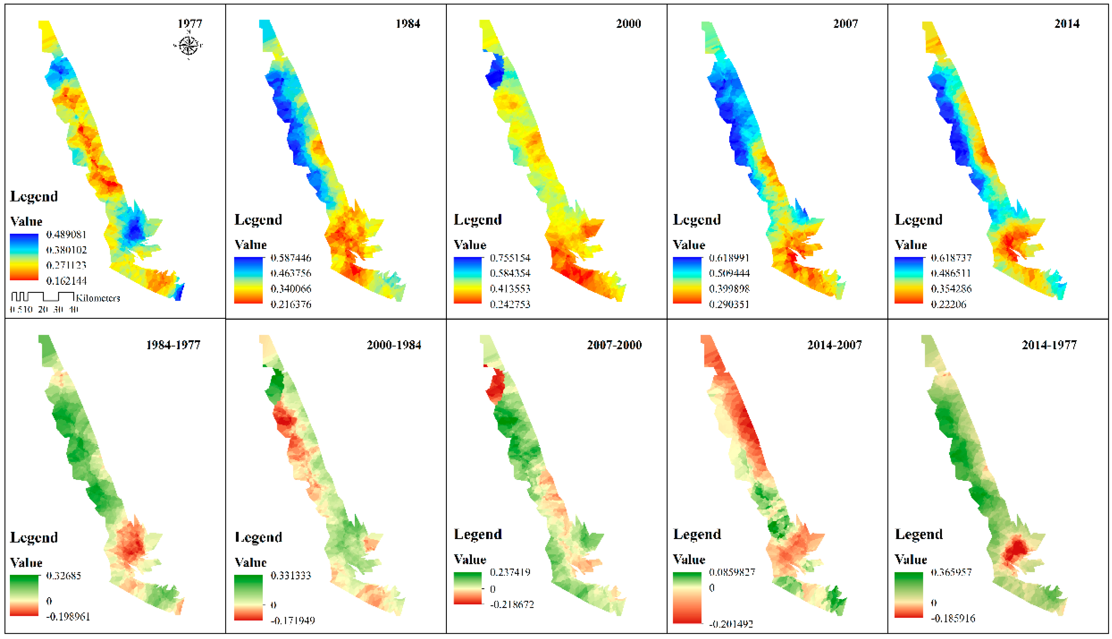
98]. Ecological security was analyzed using the theory and methodology of landscape ecology. Here the analysis was conducted at two scales: the study area scale and the cell scale. The results showed that the two scales had different features, mainly due to the scale effect [99,100,101,102]. At the cell scale, the spatiotemporal pattern of LESI showed high values located landward and low values distributed seaward. At the study area scale, the value of LESI rose in most study areas from 1977 to 2014, except in the Radial Sand Ridge of Dongtai.
Ecosystem services are the conditions and processes through which natural ecosystems, and the species that create them, sustain and fulfill human life [103]. The services of ecological systems and the natural capital stocks that produce them are critical to the functioning of the Earth’s life-support system [
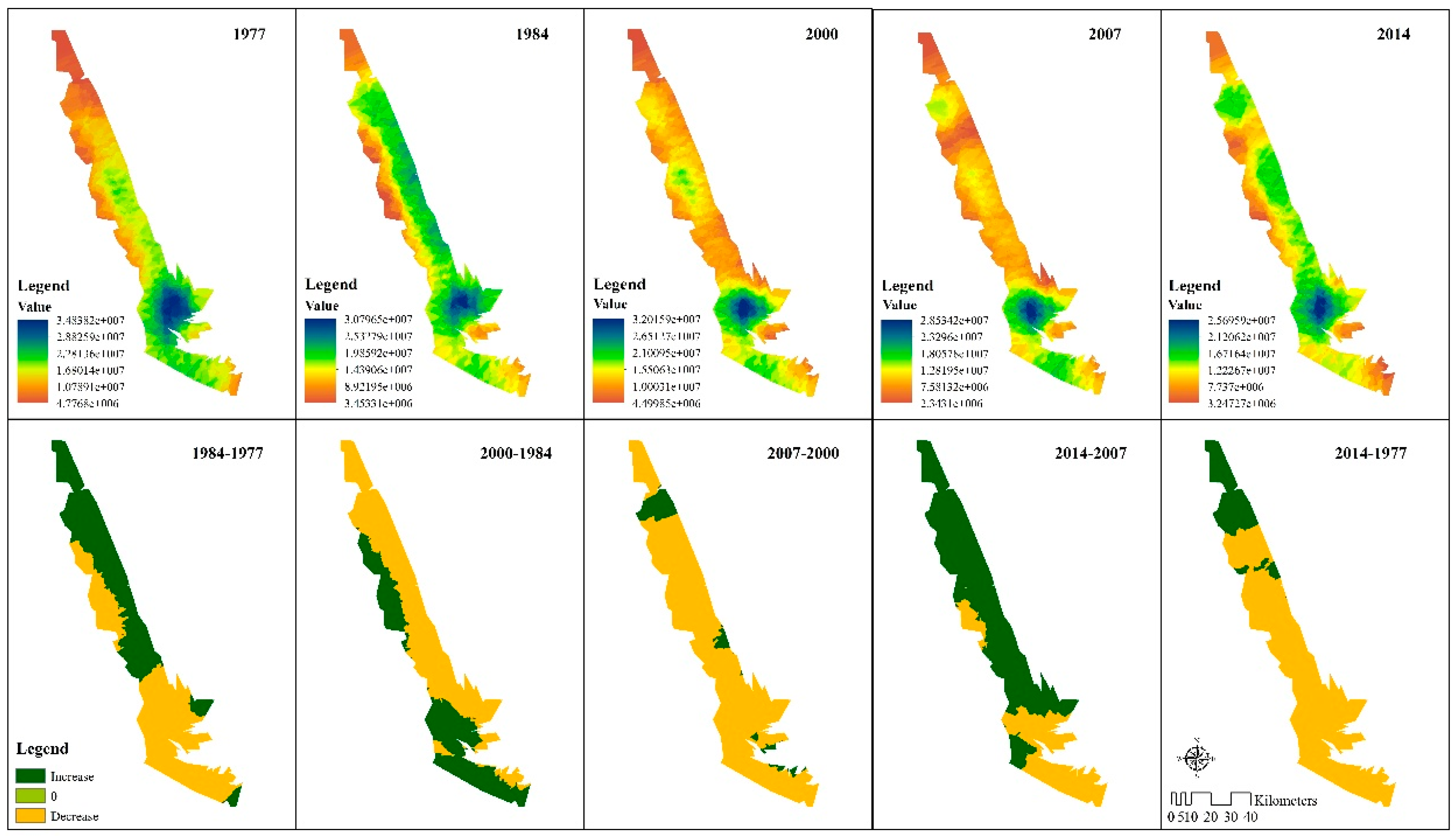
104]. With the theories of ESV and LUCC, as proposed by Costanza et al. [104] and Xie et al. [
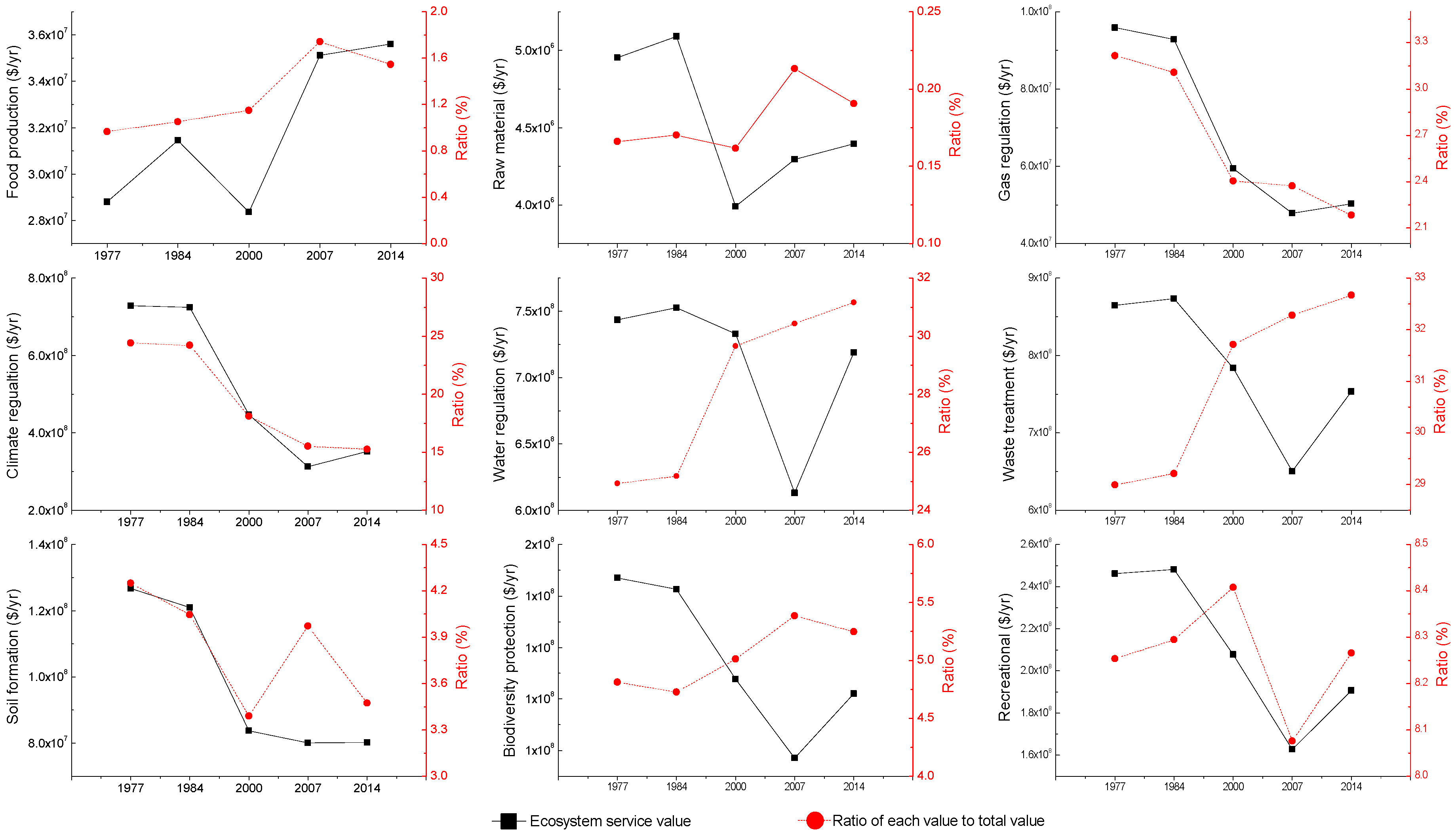
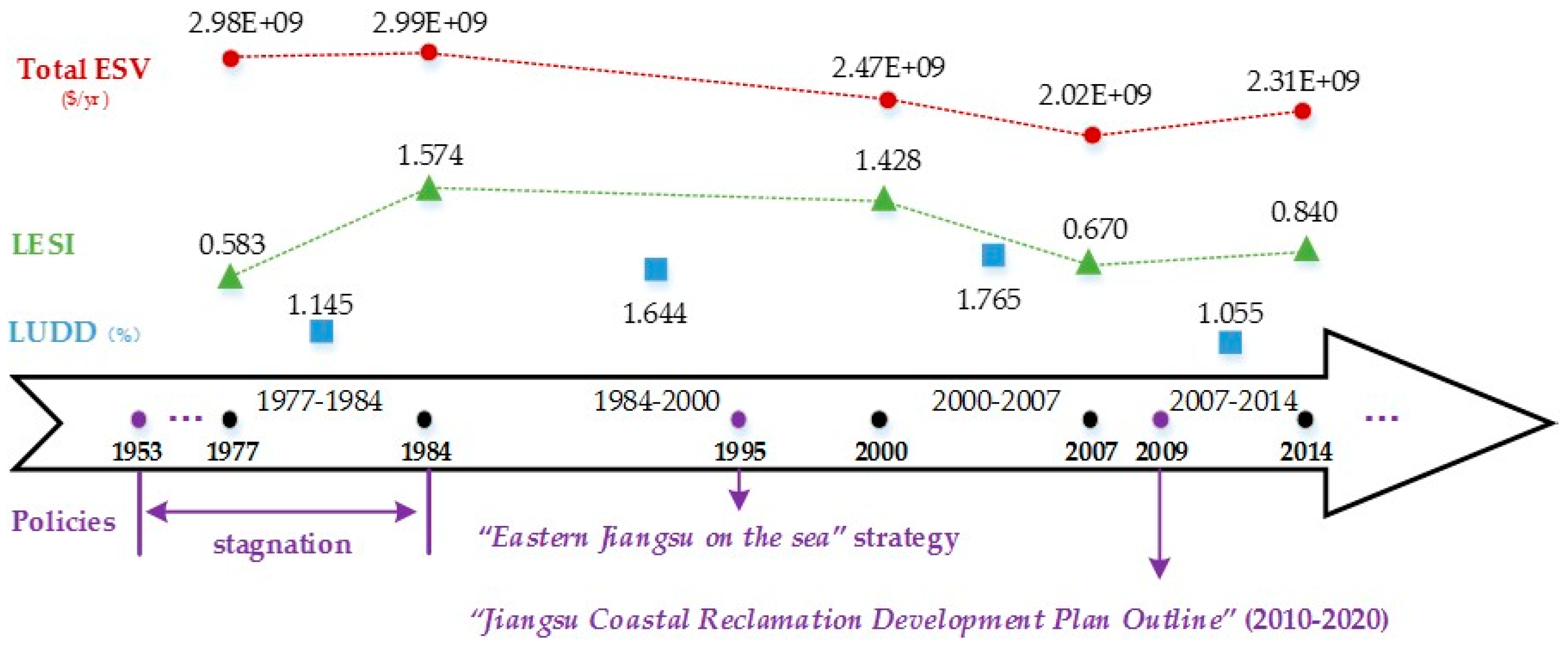
66], we found that the ESV decreased from 1977 to 2014, albeit with fluctuations, while the maximum always appeared in the Radial Sand Ridge of Dongtai. There was an average net decline of $675.96 million per year over the period 1977–2014. Furthermore, only food production had an increasing trend in 37 years. The primary reason is probably the policy in the Outline of Jiangsu Coastal Reclamation Development Plan, where the planned land use structure of reclamation zones chiefly consists of agricultural land, industrial land and ecological land, and the ratio of these is 6:2:2 [
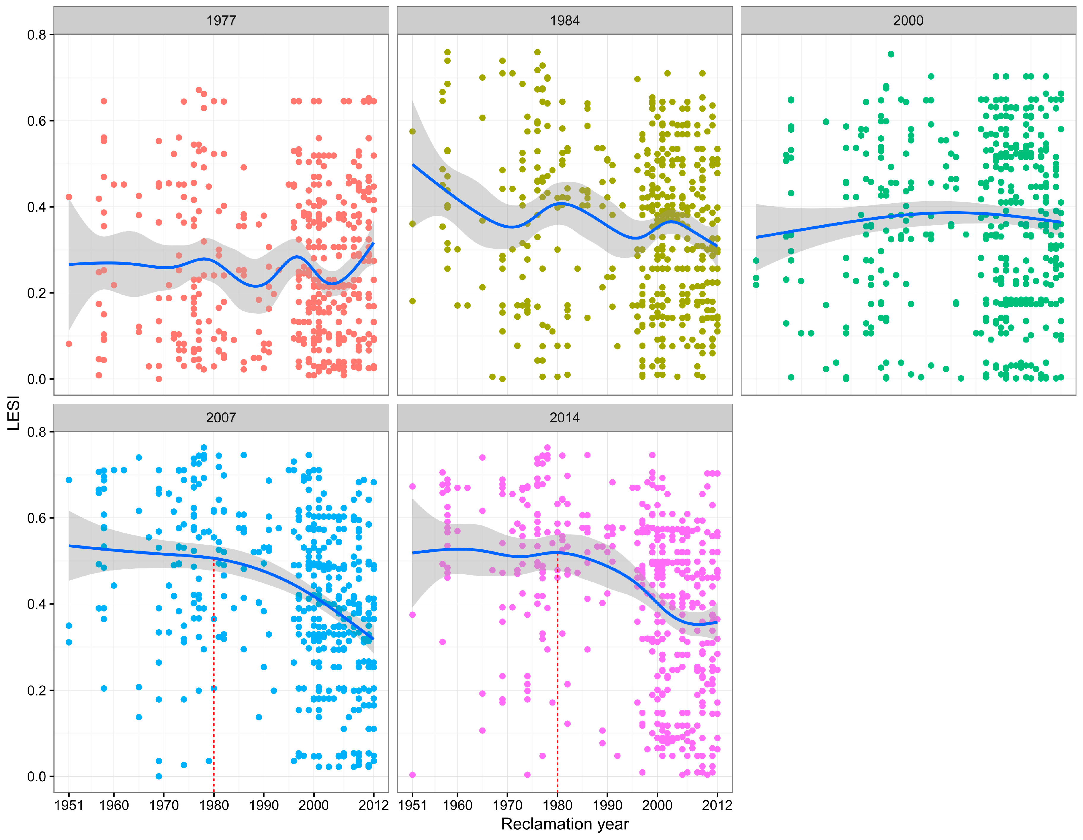
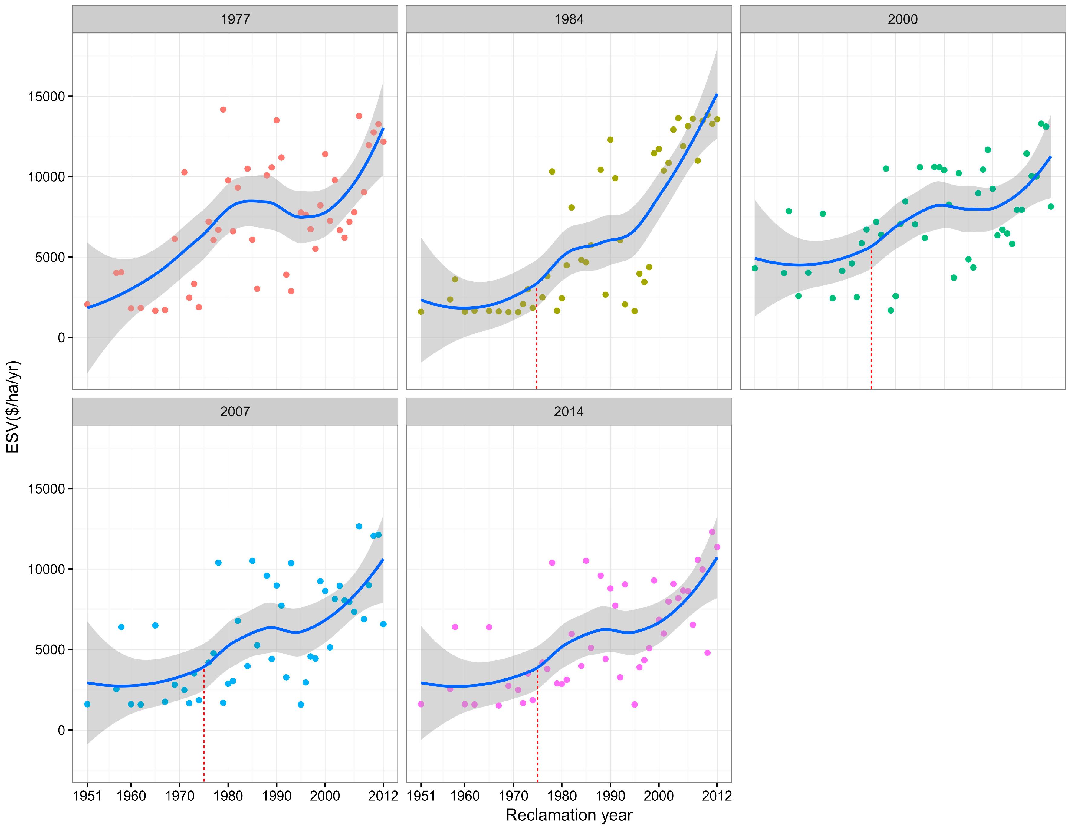
32]. This policy plays a powerful role in the growth of food production. The correlation between ESV and reclamation year showed that the ESV rapidly decreased with the reclamation year. The main reason for this result was that the artificial land use type occupied natural land, which had a high ESV. Natural land use types without human disturbance contribute more to the sustainability of wetland ecosystem than any artificial areas. Therefore, the earlier the reclamation year, the lower the ESV. This tendency appeared not only in coastal areas but also in other regions subject to human activities. For example, land use/cover changed from a natural forest to a rubber plantation in the township of Menglun, Xishuangbanna, Southwest China, resulting in a great loss of ecosystem services [105].
Rapid urbanization has simultaneously induced many adverse impacts on the environment of coastal wetland [1], not just in urban area [106]. The time required for coastal ecosystem to regain the balance was briefly discussed here from two aspects—LESI and ESV. We found that it took ~34 years for LESI and ~39 years for ESV to become balanced. Xu et al. reported that the varying features of land use in coastal reclamation areas fitted an S-type curve, and leveled off after 30 years [107]. Zhang et al. [47] suggested that 37 years was required to form an artificial system in a coastal reclamation area, which is very similar to our study. Furthermore, it has been shown that soil properties approached a relatively stable level nearly 30 years after reclamation, especially in Eastern Asia [108]. Thus, considering to our results, the coastal reclamation area would take a minimum of 30 years to recover its equilibrium.
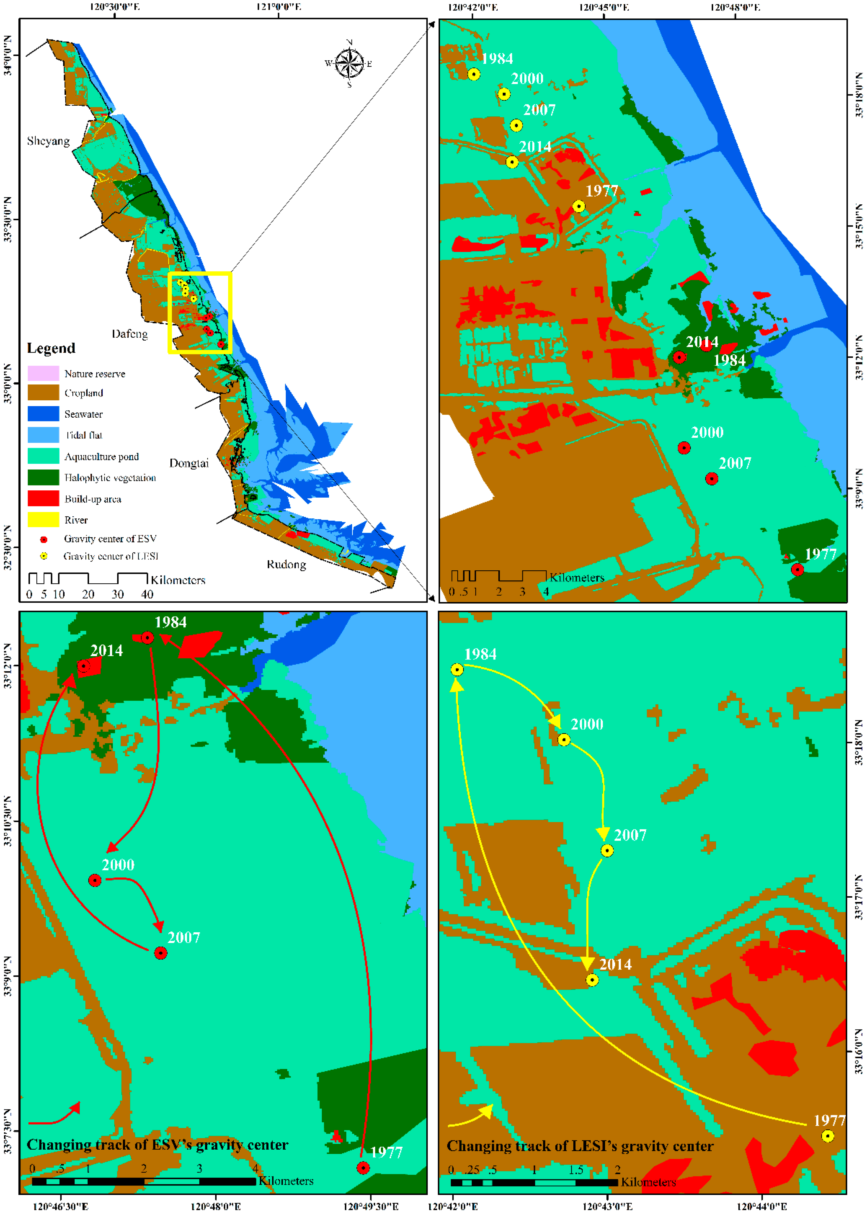
Finally, the relationship between ecological security and ecosystem services was also explored, since this area of research is typically less studied. We found the two aspects had different correlations with the different scales of the study. This was mainly because of the varying features of LESI for the two scales. The ESV was calculated based on the value method and land use change, while LESI was based on landscape ecology. We examined the spatial transformation of the gravity center. In general, both ESV and LESI both had northward changing tracks, which means that the values of LESI and ESV were increasing from south to north for the 1977–2014 period. Therefore, between 1977 and 2014, the environmental quality of the study area in the north improved to a higher level than that in the south.

5. Conclusions

China had approximately 5.8 million ha coastal wetlands in 2014, accounting for 10.82% of the total area of natural wetlands [109]. Over the past 60 years, China’s coastal wetlands have decreased enormously due to the increasing threats and pressures on wetlands arising from the growing population and rapidly developing economy [109,110]. “Jiangsu Coastal Reclamation Development Plan Outline” may be a signal that there are large and broad scale development projects to be launched in the Jiangsu coastal area in the future. Therefore, the Jiangsu coastal wetland is a key area that may experience severe land-use and eco-environment quality changes. In this research, the results can be summarized as follows:
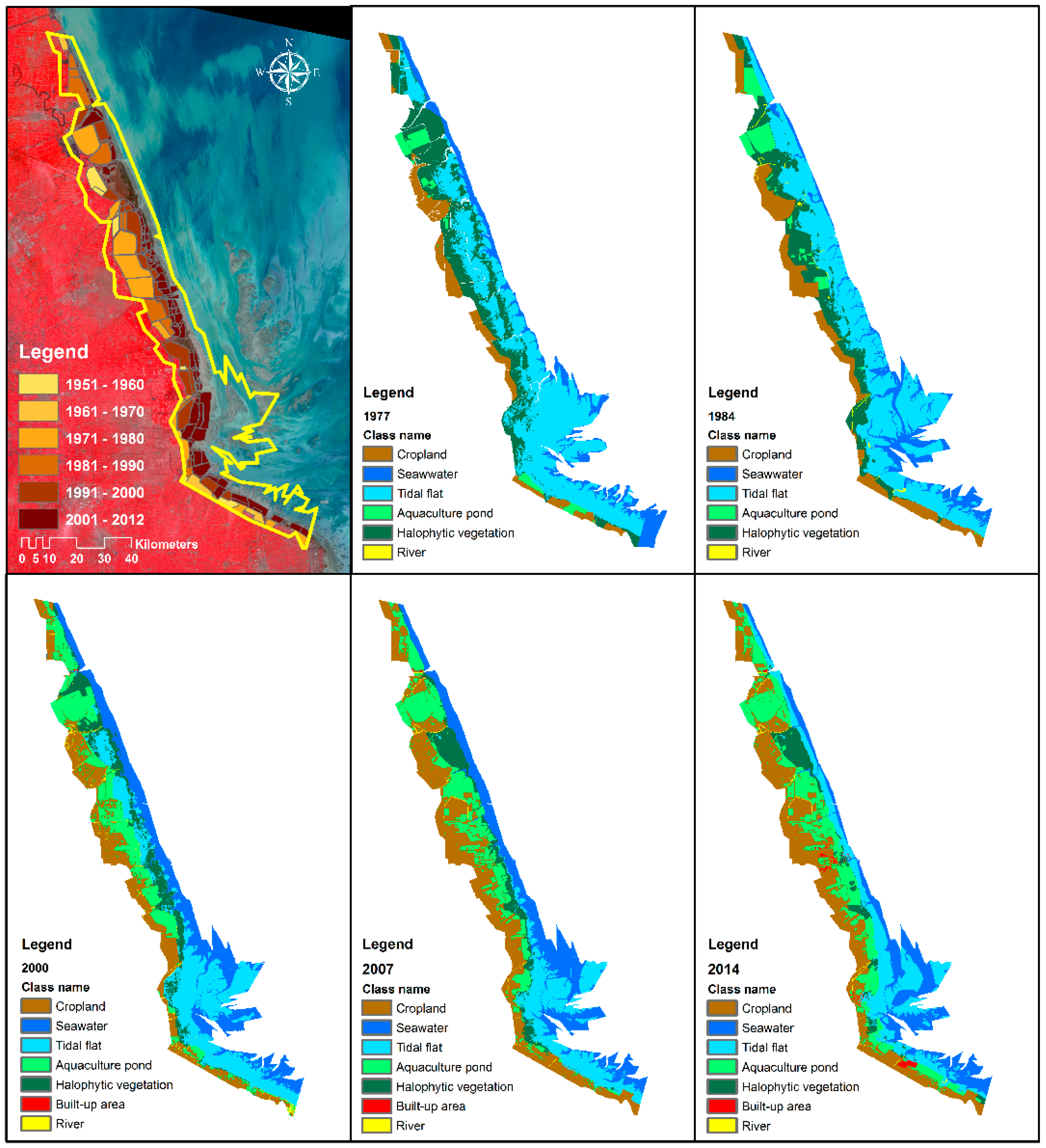
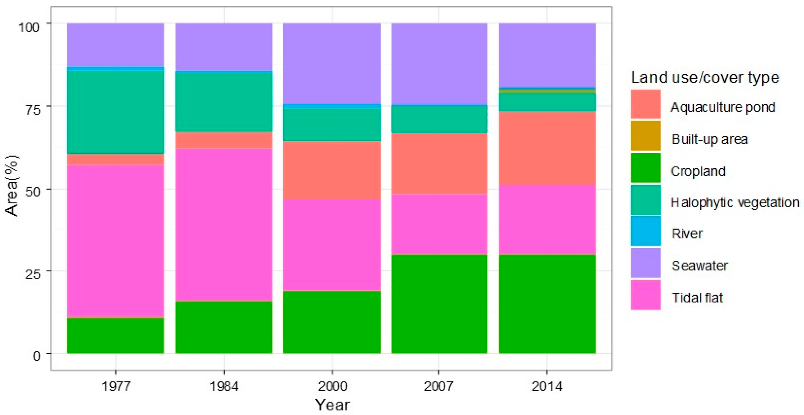
(1) The features of land use change in Jiangsu coastal area were in accordance with the most of development zones: artificial area with an increasing trend and native area with a decreasing trend. The former class contained cropland, aquaculture ponds, built-up areas, and seawater. The later class included tidal flats, halophytic vegetation, and rivers. These variations emphasize a drastic increase in production-orientated land uses and a concomitant decrease in the ecologically important wetlands. Being an ecologically fragile zone, Jiangsu coastal area should receive adequate attention.
(2) Intensive human activities break the ecological balance of coastal wetland ecosystem. According to the relationship between LESI/ESV and reclamation year as well as land use and soil quality, it could be concluded that the coastal reclamation area would recover its equilibrium after 30 years at least.
(3) In the development of coastal area, the policy is the key driving force. The total ecosystem service value declined significantly from $2.98 billion per year to $2.31 billion per year over the period 1977–2014. Food production was the only one ecosystem service function that had an increasing trend mainly because of government policy.
(4) The relationship between landscape ecological security and ecosystem service is complicated and requires further research. The main cause of the complexity is attributable to the scale effect of landscape ecology. Through the spatial analysis of the gravity center, both landscape ecological security and ecosystem services showed that the environmental quality northward became better than the south in the study period. Thus, at large scales, ecological security and ecosystem service had the same trend.

Acknowledgments

This research was supported by the National Natural Science Foundation of China (No. 41230751).

Author Contributions

Lijie Pu and Caiyao Xu conceived and designed the experiments; Caiyao Xu and Ming Zhu performed the experiments; Caiyao Xu, Jianguo Li and Xinjian Chen analyzed the data; Xiaohan Wang and Xuefeng Xie contributed analysis tools; Caiyao Xu wrote the paper. All authors have read and approved the final manuscript.

Conflicts of Interest

The authors declare no conflict of interest.

Abbreviations

The following abbreviations are used in this manuscript:
LESlandscape ecological security
LESIlandscape ecological security index
ESVecosystem service value
LUCCland use and cover change
LUDDland use dynamic degree
PDpatch density
SPLITsplitting index
FRACfractal dimension
SHDIShannon’s diversity index
SHEIShannon’s evenness index
LVIlandscape vulnerability index
LDIlandscape disturbance index
LOWESS/LOESSlocally weighted scatterplot smoothing

References

  1. Lee, S.Y.; Dunn, R.J.K.; Young, R.A.; Connolly, R.M.; Dale, P.; Dehayr, R.; Lemckert, C.J.; McKinnon, S.; Powell, B.; Teasdale, P. Impact of urbanization on coastal wetland structure and function. Austral Ecol. 2006, 31, 149–163. [Google Scholar] [CrossRef]
  2. McDonnell, M.J.; Pickett, S.T.A.; Groffman, P.; Bohlen, P.; Pouyat, R.V.; Zipperer, W.C.; Parmelee, R.W.; Carreiro, M.M.; Medley, K. Ecosystem processes along an urban-to-rural gradient. Urban Ecosyst. 1997, 1, 21–36. [Google Scholar] [CrossRef]
  3. Grimm, N.B.; Grove, J.G.; Pickett, S.T.A.; Redman, C.L. Integrated approaches to long-term studies of urban ecological systems: Urban ecological systems present multiple challenges to ecologists—Pervasive human impact and extreme heterogeneity of cities, and the need to integrate social and ecological approaches, concepts, and theory. BioScience 2000, 50, 571–584. [Google Scholar]
  4. Pickett, S.T.A.; Cadenasso, M.L.; Grove, J.M.; Nilon, C.H.; Pouyat, R.V.; Zipperer, W.C.; Costanza, R. Urban ecological systems: Linking terrestrial ecological, physical, and socioeconomic components of metropolitan areas. Annu. Rev. Ecol. Syst. 2001, 32, 127–157. [Google Scholar] [CrossRef]
  5. McKinney, M.L. Urbanization, biodiversity, and conservation: The impacts of urbanization on native species are poorly studied, but educating a highly urbanized human population about these impacts can greatly improve species conservation in all ecosystems. BioScience 2002, 52, 883–890. [Google Scholar] [CrossRef]
  6. Turner, R.K.; Subak, S.; Adger, W.N. Pressures, trends, and impacts in coastal zones: Interactions between socioeconomic and natural systems. Environ. Manag. 1996, 20, 159–173. [Google Scholar] [CrossRef]
  7. King, R.S.; Deluca, W.V.; Whigham, D.F.; Marra, P.P. Threshold effects of coastal urbanization on phragmites australis (common reed) abundance and foliar nitrogen in chesapeake bay. Estuar. Coasts 2007, 30, 469–481. [Google Scholar] [CrossRef]
  8. Charles, W.F.; Charlier, R.H. Sustainability of subtropical coastal zones in southeastern florida: Challenges for urbanized coastal environments threatened by development, pollution, water supply, and storm hazards. J. Coast. Res. 2003, 19, 934–943. [Google Scholar]
  9. Zedler, J.B.; Kercher, S. Causes and consequences of invasive plants in wetlands: Opportunities, opportunists, and outcomes. Crit. Rev. Plant Sci. 2004, 23, 431–452. [Google Scholar] [CrossRef]
  10. Zhou, H.-X.; Liu, J.-E.; Qin, P. Impacts of an alien species (Spartina alterniflora) on the macrobenthos community of Jiangsu coastal inter-tidal ecosystem. Ecol. Eng. 2009, 35, 521–528. [Google Scholar] [CrossRef]
  11. Lambin, E.F.; Turner, B.L.; Geist, H.J.; Agbola, S.B.; Angelsen, A.; Bruce, J.W.; Coomes, O.T.; Dirzo, R.; Fischer, G.; Folke, C. The causes of land-use and land-cover change: Moving beyond the myths. Glob. Environ. Chang. 2001, 11, 261–269. [Google Scholar] [CrossRef]
  12. Worrall, F.; Burt, T. The impact of land-use change on water quality at the catchment scale: The use of export coefficient and structural models. J. Hydrol. 1999, 221, 75–90. [Google Scholar] [CrossRef]
  13. Islam, K.; Weil, R. Land use effects on soil quality in a tropical forest ecosystem of Bangladesh. Agric. Ecosyst. Environ. 2000, 79, 9–16. [Google Scholar] [CrossRef]
  14. Kremen, C.; Williams, N.M.; Aizen, M.A.; Gemmill-Herren, B.; LeBuhn, G.; Minckley, R.; Packer, L.; Potts, S.G.; Steffan-Dewenter, I.; Vazquez, D.P. Pollination and other ecosystem services produced by mobile organisms: A conceptual framework for the effects of land-use change. Ecol. Lett. 2007, 10, 299–314. [Google Scholar] [CrossRef] [PubMed]
  15. Metzger, M.; Rounsevell, M.; Acosta-Michlik, L.; Leemans, R.; Schröter, D. The vulnerability of ecosystem services to land use change. Agric. Ecosyst. Environ. 2006, 114, 69–85. [Google Scholar] [CrossRef]
  16. Turner, B.L. Local faces, global flows: The role of land use and land cover in global environmental change. Land Degrad. Dev. 1994, 5, 71–78. [Google Scholar] [CrossRef]
  17. Kalnay, E.; Cai, M. Impact of urbanization and land-use change on climate. Nature 2003, 423, 528–531. [Google Scholar] [CrossRef] [PubMed]
  18. IPCC. Climate Change 2001: The Scientific Basis; Cambridge University Press: Cambridge, UK, 2001. [Google Scholar]
  19. IPCC. Climate Change 2007: The Physical Science Basis. Contribution of Working Group I to the Fourth Assessment Report of the Intergovernmental Panel on Climate Change; Cambridge University Press: Cambridge, UK, 2007. [Google Scholar]
  20. IPCC. Climate Change 2014: Synthesis Report. Contribution of Working Groups I, II and III to the Fifth Assessment Report of the Intergovernmental Panel on Climate Change; IPCC: Geneva, Switzerland, 2014. [Google Scholar]
  21. Jeanson, M.; Dolique, F.; Anthony, E.J. A GIS-based coastal monitoring and surveillance observatory on tropical islands exposed to climate change and extreme events: The example of Mayotte Island, Indian ocean. J. Coast. Conserv. 2014, 18, 567–580. [Google Scholar] [CrossRef]
  22. Parthasarathy, A.; Natesan, U. Coastal vulnerability assessment: A case study on erosion and coastal change along Tuticorin, Gulf of Mannar. Nat. Hazards 2015, 75, 1713–1729. [Google Scholar] [CrossRef]
  23. Islam, A.M.; Mitra, D.; Dewan, A.; Akhter, S.H. Coastal multi-hazard vulnerability assessment along the ganges deltaic coast of Bangladesh—A geospatial approach. Ocean Coast. Manag. 2016, 127, 1–15. [Google Scholar] [CrossRef]
  24. Hereher, M.E. Assessment of Egypt’s red sea coastal sensitivity to climate change. Environ. Earth Sci. 2015, 74, 2831–2843. [Google Scholar] [CrossRef]
  25. Boruff, B.J.; Emrich, C.; Cutter, S.L. Erosion hazard vulnerability of US coastal counties. J. Coast. Res. 2005, 21, 932–942. [Google Scholar] [CrossRef]
  26. An, S.; Li, H.; Guan, B.; Zhou, C.; Wang, Z.; Deng, Z.; Zhi, Y.; Liu, Y.; Xu, C.; Fang, S.; et al. China’s natural wetlands: Past problems, current status, and future challenges. Ambio 2007, 36, 335–342. [Google Scholar] [CrossRef]
  27. Wolff, W.J. The end of a tradition: 1000 years of embankment and reclamation of wetlands in the Netherlands. Ambio 1992, 21, 287–291. [Google Scholar]
  28. Ohkura, Y. The roles and limitations of newspapers in environmental reporting. Case study: Isahaya Bay land reclamation project issue. Mar. Pollut. Bull. 2003, 47, 237–245. [Google Scholar] [CrossRef]
  29. Lie, H.-J.; Cho, C.-H.; Lee, S.; Kim, E.-S.; Koo, B.-J.; Noh, J.-H. Changes in marine environment by a large coastal development of the saemangeum reclamation project in Korea. Ocean Polar Res. 2008, 30, 475–484. [Google Scholar] [CrossRef]
  30. Wang, W.; Liu, H.; Li, Y.; Su, J. Development and management of land reclamation in China. Ocean Coast. Manag. 2014, 102, 415–425. [Google Scholar] [CrossRef]
  31. Ma, Z.; Melville, D.S.; Liu, J.; Chen, Y.; Yang, H.; Ren, W.; Zhang, Z.; Piersma, T.; Li, B. Rethinking China’s new Great Wall. Science 2014, 346, 912–914. [Google Scholar] [CrossRef] [PubMed]
  32. The People’s Government of Jiangsu Province. Jiangsu Beach Reclamation Development Planning Outline. Available online: http://govinfo.nlc.gov.cn/jssfz/jszb/201020/201104/t20110414_696110.shtml?classid=416# (accessed on 16 August 2016). (In Chinese)
  33. Gao, J.; Bai, F.; Yang, Y.; Gao, S.; Liu, Z.; Li, J. Influence of spartina colonization on the supply and accumulation of organic carbon in tidal salt marshes of northern Jiangsu Province, China. J. Coast. Res. 2012, 486–498. [Google Scholar] [CrossRef]
  34. Yao, H. Characterizing landuse changes in 1990–2010 in the coastal zone of Nantong, Jiangsu Province, China. Ocean Coast. Manag. 2013, 71, 108–115. [Google Scholar] [CrossRef]
  35. Liao, H.; Li, G.; Cui, L.; Ouyang, N.; Zhang, Y.; Wang, S. Study on evolution features and spatial distribution patterns of coastal wetlands in north Jiangsu Province, China. Wetlands 2014, 34, 877–891. [Google Scholar] [CrossRef]
  36. Liu, X.J.; Gao, S.; Wang, Y.P. Modeling the deposition system evolution of accreting tidal flats: A case study from the coastal plain of central Jiangsu, China. J. Coast. Res. 2015, 31, 107–118. [Google Scholar] [CrossRef]
  37. Tang, D.; Zou, X.; Liu, X.; Liu, P.; Zhamangulova, N.; Xu, X.; Zhao, Y. Integrated ecosystem health assessment based on eco-exergy theory: A case study of the Jiangsu coastal area. Ecol. Indic. 2015, 48, 107–119. [Google Scholar] [CrossRef]
  38. Naveh, Z.; Lieberman, A.S. Landscape Ecology: Theory and Application; Springer Science & Business Media: Berlin, Germany, 2013. [Google Scholar]
  39. Wu, J.G. Landscape ecology, cross-disciplinarity, and sustainability science. Landsc. Ecol. 2006, 21, 1–4. [Google Scholar] [CrossRef]
  40. O’Neill, R.V.; Krummel, J.R.; Gardner, R.H.; Sugihara, G.; Jackson, B.; DeAngelis, D.L.; Milne, B.T.; Turner, M.G.; Zygmunt, B.; Christensen, S.W.; et al. Indices of landscape pattern. Landsc. Ecol. 1988, 1, 153–162. [Google Scholar] [CrossRef]
  41. McGarigal, K.; Marks, B.J. Fragstats: Spatial Pattern Analysis Program for Quantifying Landscape Structure; Gen. Tech. Rep. PNW-GTR-351; US Department of Agriculture, Forest Service, Pacific Northwest Research Station: Portland, OR, USA, 1995.
  42. Hargis, C.D.; Bissonette, J.A.; David, J.L. The behavior of landscape metrics commonly used in the study of habitat fragmentation. Lands. Ecol. 1998, 13, 167–186. [Google Scholar] [CrossRef]
  43. O’Neill, R.V.; Riitters, K.H.; Wickham, J.D.; Jones, K.B. Landscape pattern metrics and regional assessment. Ecosyst. Health 1999, 5, 225–233. [Google Scholar] [CrossRef]
  44. Luck, M.; Wu, J.G. A gradient analysis of urban landscape pattern: A case study from the Phoenix metropolitan region, Arizona, USA. Landsc. Ecol. 2002, 17, 327–339. [Google Scholar] [CrossRef]
  45. Tzanopoulos, J.; Vogiatzakis, I.N. Processes and patterns of landscape change on a small Aegean island: The case of Sifnos, Greece. Landsc. Urban Plan. 2011, 99, 58–64. [Google Scholar] [CrossRef]
  46. Dewan, A.M.; Yamaguchi, Y.; Ziaur Rahman, M. Dynamics of land use/cover changes and the analysis of landscape fragmentation in Dhaka metropolitan, Bangladesh. GeoJournal 2012, 77, 315–330. [Google Scholar] [CrossRef]
  47. Zhang, R.S.; Pu, L.J.; Li, J.G.; Zhang, J.; Xu, Y. Landscape ecological security response to land use change in the tidal flat reclamation zone, China. Environ. Monit. Assess. 2016, 188, 1–10. [Google Scholar] [CrossRef] [PubMed]
  48. Gao, Y.; Wu, Z.; Lou, Q.; Huang, H.; Cheng, J.; Chen, Z. Landscape ecological security assessment based on projection pursuit in Pearl River Delta. Environ. Monit. Assess. 2012, 184, 2307–2319. [Google Scholar] [CrossRef] [PubMed]
  49. Huang, J.; Wang, R.; Zhang, H. Analysis of patterns and ecological security trend of modern oasis landscapes in Xinjiang, China. Environ. Monit. Assess. 2007, 134, 411–419. [Google Scholar] [CrossRef] [PubMed]
  50. Botequilha Leitão, A.; Ahern, J. Applying landscape ecological concepts and metrics in sustainable landscape planning. Landsc. Urban Plan. 2002, 59, 65–93. [Google Scholar] [CrossRef]
  51. Berger, J. Guidelines for landscape synthesis: Some directions—Old and new. Landsc. Urban Plan. 1987, 14, 295–311. [Google Scholar] [CrossRef]
  52. Xie, Z.; Xu, L.; Duan, X.; Xu, X. Analysis of boundary adjustments and land use policy change—A case study of Tianjin Palaeocoast and Wetland National Natural Reserve, China. Ocean Coast. Manag. 2012, 56, 56–63. [Google Scholar] [CrossRef]
  53. Zhang, R.; Lu, L.; Wang, Y. The mechanism and trend of coastal erosion of Jiangsu Province in China. Geogr. Res. 2002, 21, 469–478. [Google Scholar]
  54. Zhao, S.-S.; Liu, Y.-X.; Li, M.-C.; Sun, C.; Zhou, M.-X.; Zhang, H.-X. Analysis of Jiangsu tidal flats reclamation from 1974 to 2012 using remote sensing. China Ocean Eng. 2015, 29, 143–154. [Google Scholar] [CrossRef]
  55. Li, J.; Pu, L.; Zhu, M.; Dai, X.; Xu, Y.; Chen, X.; Zhang, L.; Zhang, R. Monitoring soil salt content using HJ-1A hyperspectral data: A case study of coastal areas in Rudong County, eastern China. Chin. Geogr. Sci. 2015, 25, 213–223. [Google Scholar] [CrossRef]
  56. Hatch, L.K.; Mallawatantri, A.; Wheeler, D.; Gleason, A.; Mulla, D.; Perry, J.; Easter, K.W.; Smith, R.; Gerlach, L.; Brezonik, P. Land management at the major watershed—Agroecoregion intersection. J. Soil Water Conserv. 2001, 56, 44–51. [Google Scholar]
  57. Sun, Y.; Li, X.; Mander, Ü.; He, Y.; Jia, Y.; Ma, Z.; Guo, W.; Xin, Z. Effect of reclamation time and land use on soil properties in Changjiang River estuary, China. Chin. Geogr. Sci. 2011, 21, 403–416. [Google Scholar] [CrossRef]
  58. China Centre for Resources Satellite Data and Application. Available online: http://www.cresda.com/CN/ (accessed on 16 August 2016). (In Chinese)
  59. Chinese Academy of Sciences Computer Network Information Center. Geospatial Data Cloud. Available online: http://www.gscloud.cn/ (accessed on 16 August 2016). (In Chinese)
  60. Yang, S.; Yan, H.; Guo, L. The land use change and its eco-environmental effects in transitional agro-pastoral region—A case study of Yulin City in northern Shaanxi Province. Prog. Geogr. 2004, 23, 49–55. [Google Scholar]
  61. Wang, X.; Bao, Y. Study on the methods of land use dynamic change research. Prog. Geogr. 1999, 18, 83–89. [Google Scholar]
  62. Han, Z.; Li, J.; Yin, H.; Yajin, S.; Xu, C. Analysis of ecological security of wetland in Liaohe River Delta based on the landscape pattern. Ecol. Environ. Sci. 2010, 19, 701–705. [Google Scholar]
  63. Gao, Y.; Huang, H.; Wu, Z. Landscape ecological security assessment based on projection pursuit: A case study of nine cities in the Pearl River Delta. Acta Ecol. Sin. 2010, 30, 5894–5903. [Google Scholar]
  64. Juan, W.; BaoShan, C.U.I.; HuaRong, Y.A.; ShiLiang, L.I.U. The temporal and spatial characteristic of landscape ecological security at lancang river watershed of longitudinal range gorge region in southwest China. Acta Ecol. Sin. 2008, 28, 1681–1690. [Google Scholar]
  65. McGarigal, K.; Cushman, S.; Maile, N.; Ene, E. FRAGSTATS v4: Spatial Pattern Analysis Program for Categorical and Continuous Maps; Department of Environmental Conservation, University of Massachusetts: Amherst, MA, USA, 2012. [Google Scholar]
  66. Xie, G.; Lu, C.; Leng, Y.; Zheng, D.; Li, S. Ecological assets valuation of the Tibetan Plateau. J. Nat. Resour. 2003, 18, 189–196. [Google Scholar]
  67. Jiangsu Province’s Bureau of Statistics. Jiangsu Statistical Yearbook. Available online: http://www.jssb.gov.cn/ (accessed on 16 August 2016). (In Chinese)
  68. Food and Agriculture Organization of the United Nations. Available online: http://faostat3.fao.org/download/P/PP/E (accessed on 16 August 2016).
  69. Kreuter, U.P.; Harris, H.G.; Matlock, M.D.; Lacey, R.E. Change in ecosystem service values in the San Antonio area, Texas. Ecol. Econ. 2001, 39, 333–346. [Google Scholar] [CrossRef]
  70. He, Y.; Chen, Y.; Tang, H.; Yao, Y.; Yang, P.; Chen, Z. Exploring spatial change and gravity center movement for ecosystem services value using a spatially explicit ecosystem services value index and gravity model. Environ. Monit. Assess. 2011, 175, 563–571. [Google Scholar] [CrossRef] [PubMed]
  71. Sen, A.; Smith, T. Gravity Models of Spatial Interaction Behavior; Springer Science & Business Media: Berlin, Germany, 2012. [Google Scholar]
  72. Sun, D.; Zhang, J.; Zhu, C.; Hu, Y.; Zhou, L. An assessment of China’s ecological environment quality change and its spatial variation. Acta Geogr. Sin. 2012, 67, 1599–1610. [Google Scholar]
  73. Earls, J.; Dixon, B. Spatial interpolation of rainfall data using ArcGIS: A comparative study. In Proceedings of the 27th Annual ESRI International User Conference, San Diego, CA, USA, 18–22 June 2007.
  74. Mishra, U.; Lal, R.; Slater, B.; Calhoun, F.; Liu, D.; van Meirvenne, M. Predicting soil organic carbon stock using profile depth distribution functions and ordinary kriging. Soil Sci. Soc. Am. J. 2009, 73, 614–621. [Google Scholar] [CrossRef]
  75. Childs, C. Interpolating Surfaces in ArcGIS Spatial Analyst. Available online: http://www.esri.com/news/arcuser/0704/files/interpolating.pdf (accessed on 17 July 2016).
  76. Dubrule, O. Two methods with different objectives: Splines and kriging. J. Int. Assoc. Math. Geol. 1983, 15, 245–257. [Google Scholar] [CrossRef]
  77. Dubrule, O. Comparing splines and kriging. Comput. Geosci. 1984, 10, 327–338. [Google Scholar] [CrossRef]
  78. Laslett, G.; McBratney, A.; Pahl, P.J.; Hutchinson, M. Comparison of several spatial prediction methods for soil pH. J. Soil Sci. 1987, 38, 325–341. [Google Scholar] [CrossRef]
  79. Oliver, M.A.; Webster, R. Kriging: A method of interpolation for geographical information systems. Int. J. Geogr. Inf. Syst. 1990, 4, 313–332. [Google Scholar] [CrossRef]
  80. Laslett, G.M. Kriging and splines: An empirical comparison of their predictive performance in some applications. J. Am. Stat. Assoc. 1994, 89, 391–400. [Google Scholar] [CrossRef]
  81. Zhu, Q.; Lin, H.S. Comparing ordinary kriging and regression kriging for soil properties in contrasting landscapes. Pedosphere 2010, 20, 594–606. [Google Scholar] [CrossRef]
  82. Cleveland, W.S.; Devlin, S.J. Locally weighted regression: An approach to regression analysis by local fitting. J. Am. Stat. Assoc. 1988, 83, 596–610. [Google Scholar] [CrossRef]
  83. Cleveland, W.S. Lowess: A program for smoothing scatterplots by robust locally weighted regression. Am. Stat. 1981. [Google Scholar] [CrossRef]
  84. Cleveland, W.S. Robust locally weighted regression and smoothing scatterplots. J. Am. Stat. Assoc. 1979, 74, 829–836. [Google Scholar] [CrossRef]
  85. McArthur, J.; Howarth, R.; Bailey, T. Strontium isotope stratigraphy: LOWESS version 3: Best fit to the marine Sr-isotope curve for 0–509 ma and accompanying look-up table for deriving numerical age. J. Geol. 2001, 109, 155–170. [Google Scholar] [CrossRef]
  86. Yan, Y.-G. On history and status of costal economic development in Jiangsu Province. J. Jiangsu Polytech. Univ. (Soc. Sci. Ed.) 2008, 9, 37–41. (In Chinese) [Google Scholar]
  87. Alphan, H. Land-use change and urbanization of Adana, Turkey. Land Degrad. Dev. 2003, 14, 575–586. [Google Scholar] [CrossRef]
  88. López, E.; Bocco, G.; Mendoza, M.; Duhau, E. Predicting land-cover and land-use change in the urban fringe a case in Morelia city, Mexico. Landsc. Urban Plan. 2001, 55, 271–285. [Google Scholar] [CrossRef]
  89. Gu, D.; Zhang, Y.; Fu, J.; Zhang, X. The landscape pattern characteristics of coastal wetlands in Jiaozhou Bay under the impact of human activities. Environ. Monit. Assess. 2007, 124, 361–370. [Google Scholar] [CrossRef] [PubMed]
  90. Dewan, A.M.; Yamaguchi, Y. Using remote sensing and gis to detect and monitor land use and land cover change in Dhaka metropolitan of Bangladesh during 1960–2005. Environ. Monit. Assess. 2008, 150, 237–249. [Google Scholar] [CrossRef] [PubMed]
  91. Dabelko, G.D.; Dabelko, D.D. Environmental security: Issues of conflict and redefinition. Environ. Chang. Secur. Proj. Rep. 1995, 1, 3–13. [Google Scholar]
  92. Levy, M.A. Is the environment a national security issue? Int. Secur. 1995, 20, 35–62. [Google Scholar] [CrossRef]
  93. Rogers, K.S. Ecological security and multinational corporations. Environ. Chang. Secur. Proj. Rep. 1997, 3, 29–36. [Google Scholar]
  94. Solovjova, N.V. Synthesis of ecosystemic and ecoscreening modelling in solving problems of ecological safety. Ecol. Model. 1999, 124, 1–10. [Google Scholar] [CrossRef]
  95. Ezeonu, I.C.; Ezeonu, F.C. The environment and global security. Environmentalist 2000, 20, 41–48. [Google Scholar] [CrossRef]
  96. Dalby, S. Security and ecology in the age of globalization. Environ. Chang. Secur. Proj. Rep. 2002, 8, 95–108. [Google Scholar]
  97. Kullenberg, G. Regional co-development and security: A comprehensive approach. Ocean Coast. Manag. 2002, 45, 761–776. [Google Scholar] [CrossRef]
  98. Li, X.; Ma, K.; Fu, B.; Niu, S. The regional pattern for ecological security (RPES): Designing principles and method. Acta Ecol. Sin. 2004, 24, 1055–1062. [Google Scholar]
  99. Turner, M.G. Landscape ecology: The effect of pattern on process. Annu. Rev. Ecol. Syst. 1989, 20, 171–197. [Google Scholar] [CrossRef]
  100. Turner, M.G.; O’Neill, R.V.; Gardner, R.H.; Milne, B.T. Effects of changing spatial scale on the analysis of landscape pattern. Landsc. Ecol. 1989, 3, 153–162. [Google Scholar] [CrossRef]
  101. Wu, J. Effects of changing scale on landscape pattern analysis: Scaling relations. Landsc. Ecol. 2004, 19, 125–138. [Google Scholar] [CrossRef]
  102. Pickett, S.T.; Cadenasso, M.L. Landscape ecology: Spatial heterogeneity in ecological systems. Science 1995, 269, 331–334. [Google Scholar] [CrossRef] [PubMed]
  103. Daily, G. Nature’s Services: Societal Dependence on Natural Ecosystems; Island Press: Washington, DC, USA, 1997. [Google Scholar]
  104. Costanza, R.; d’Arge, R.; de Groot, R.; Farber, S.; Grasso, M.; Hannon, B.; Limburg, K.; Naeem, S.; O’Neill, R.V.; Paruelo, J.; et al. The value of the world’s ecosystem services and natural capital. Nature 1997, 387, 253–260. [Google Scholar] [CrossRef]
  105. Hu, H.; Liu, W.; Cao, M. Impact of land use and land cover changes on ecosystem services in Menglun, Xishuangbanna, southwest China. Environ. Monit. Assess. 2008, 146, 147–156. [Google Scholar] [CrossRef] [PubMed]
  106. Dewan, A.M.; Kabir, M.H.; Nahar, K.; Rahman, M.Z. Urbanisation and environmental degradation in Dhaka metropolitan area of Bangladesh. Int. J. Environ. Sustain. Dev. 2012, 11, 118–147. [Google Scholar] [CrossRef]
  107. Xu, Y.; Pu, L. The variation of land use pattern in tidal flat reclamation zones in Jiangsu coastal area: A case study of Rudong County of Jiangsu Province. J. Nat. Resour. 2014, 29, 643–652. [Google Scholar]
  108. Li, J.; Pu, L.; Zhu, M.; Zhang, J.; Li, P.; Dai, X.; Xu, Y.; Liu, L. Evolution of soil properties following reclamation in coastal areas: A review. Geoderma 2014, 226–227, 130–139. [Google Scholar] [CrossRef]
  109. Sun, Z.; Sun, W.; Tong, C.; Zeng, C.; Yu, X.; Mou, X. China’s coastal wetlands: Conservation history, implementation efforts, existing issues and strategies for future improvement. Environ. Int. 2015, 79, 25–41. [Google Scholar] [CrossRef] [PubMed]
  110. Pascual-Aguilar, J.; Andreu, V.; Gimeno-García, E.; Picó, Y. Current anthropogenic pressures on agro-ecological protected coastal wetlands. Sci. Total Environ. 2015, 503–504, 190–199. [Google Scholar] [CrossRef] [PubMed]
Figure 1. A brief framework of this study. Human activity results in broad change to land use and land cover. We assessed land use change with two land use dynamic degree models. Linking human activity and the ecosystem via land use change, we analyzed the variation of ecosystem services and ecological security to explore how the ecosystem responded to human activity.
Sustainability 08 00816 g001
Figure 2. The administrative region of Jiangsu central coastal zone, its location and the distribution of natural reserves in the study area. The detailed information on remote sensing images can be found in Table 1.
Sustainability 08 00816 g002
Figure 3. Classified land use/cover maps of the Jiangsu central coastal zone in 1977, 1984, 2000, 2007 and 2014.
Sustainability 08 00816 g003
Figure 4. The area of each land use/cover type in study area over the period of 1977–2014.
Sustainability 08 00816 g004
Figure 5. The land use dynamic degree of each land use/cover type and the land use integrated dynamic degree of the whole study area from 1977 to 2014.
Sustainability 08 00816 g005
Figure 6. The spatiotemporal features and dynamic variation of LESI at the cell scale over 37 years.
Sustainability 08 00816 g006
Figure 7. Relationship between LESI and reclamation year. The detailed information of the reclamation year in the study area was shown in Figure 3.
Sustainability 08 00816 g007
Figure 8. The spatiotemporal features and dynamic change of ecosystem service at the cell scale in Jiangsu central coastal zone from 1977 to 2014.
Sustainability 08 00816 g008
Figure 9. The value and ratio of each ecosystem service function in study area from 1977 to 2014.
Sustainability 08 00816 g009
Figure 10. Relationship between ESV and reclamation year. The detailed information of the reclamation year in the study area was shown in Figure 3.
Sustainability 08 00816 g010
Figure 11. Relationship between total ESV and LESI at two scales.
Sustainability 08 00816 g011
Figure 12. The changing track of LESI and ESV gravity centers.
Sustainability 08 00816 g012
Figure 13. The comprehensive comparison among ecosystem service value (ESV), landscape ecological security index (LESI), land use dynamic degree and policies with time.
Sustainability 08 00816 g013
Table 1. The parameters of remotely sensed images of the study area.
SatelliteSensorPath/RowAcquisition DateResolution/m
HJ-1BCCD450/7623 April 201430
Landsat 5TM119/3717 June 200730
Landsat 7ETM119/3720 May 200030
Landsat 5TM119/374 August 198430
Landsat 2TM128/3720 April 197779
Note: the HJ-1B remote sensing image was from China Centre for Resources Satellite Data and Application [58]; the Landsat 2–7 remote sensing images were from Geospatial Data Cloud [59].
Table 2. Descriptions of land use and land cover classes used in this study.
No.LUCC ClassDescriptionwi
1CroplandLand in either a vegetated or nonvegetated state used for the production of food and oil, including cultivated and uncultivated croplands0.6
2SeawaterPart of Yellow Sea0.7
3Tidal flatTidal flats are common along shallow-water coastlines and estuaries worldwide, accumulating fine-grained sediments on gently sloping beds, forming the basic structure upon which coastal wetlands built1
4Aquaculture pondThe farming of fish and other aquatic life in regular ponds0.5
5Halophytic vegetationGrow in salt-affected habitats with many species0.8
6Built-up areaRural residential land0.2
7RiverA large amount of fresh water flowing continuously in a long line across the land0.8
Note: wi is a parameter used in the calculation of the land vulnerability index (LVI) [60], and the LVI is used to calculate the landscape ecological security index.
Table 3. Equivalent weighting of ecosystem services per hectare of terrestrial ecosystems in China.
Ecosystem ServiceFarmlandForestGrasslandWetlandWater BodyBarren Land
ProvisioningFood production10.10.30.30.10.01
Raw material0.12.60.050.070.010
RegulatingGas regulation0.53.50.81.800
Climate regulation0.892.70.917.10.460
Water regulation0.63.20.815.520.380.03
Waste treatment1.641.311.3118.1818.180.01
SupportingSoil formation1.463.91.951.710.010.02
Biodiversity protection0.713.261.092.52.490.34
CulturalRecreational0.011.280.045.554.340.01
Total6.9121.857.2462.7145.970.42
Table 4. Ecosystem service value per hectare of the Jiangsu central coastal zone, China.
Ecosystem ServiceCroplandTidal FlatAquaculture PondHalophytic VegetationBuilt-up AreaRiver/Ditch
ProvisioningFood production230.5869.1723.0669.172.3123.06
Raw material23.0616.142.3111.530.002.31
RegulatingGas regulation115.29415.050.00184.470.000.00
Climate regulation205.223942.96106.07207.520.00106.07
Water regulation138.353574.034699.27184.476.924699.27
Waste treatment378.154191.994191.99302.062.314191.99
SupportingSoil formation336.65394.302.31449.644.612.31
Biodiversity protection163.71576.46574.15251.3378.40574.15
CulturalRecreational2.311279.731000.739.222.311000.73
Total1593.3214,459.8310,599.891669.4196.8610,599.89
Table 5. Correlation coefficient between LESI and ESV based on the cell scale.
Correlation Coefficient RESV
LESI1977−0.134
1984−0.179 *
2000−0.364 ***
2007−0.353 ***
2014−0.375 ***
Note: Levels of significance test: * p < 0.1; *** p < 0.001.

