1. Introduction
The rapid development of e-commerce has generated growing interest in online shopping. Taking China as an example, according to China’s E-commerce Report 2015 [
1], in 2015, the e-commerce transactions totaled 2.5 trillion US dollars and online shopping transactions accounted for 80% of the total e-commerce transactions with an increasing rate of 27.2% compared to 2014. The sharply increased online shopping market leads to an explosive growth of city distribution demand. The annual package delivery quantity reached 20 billion in 2015, leading China to rank first in the world. The Last Mile delivery works as the final stretch that delivers consignments to the recipients [
2] and plays an indispensable role in promoting e-commerce development. A survey showed that 85% of buyers who received their orders on time would purchase online again compared with those 33% who received delayed orders [
3]. Different to traditional city distribution, the customers engaging in online shopping are spatially distributed and have personalized delivery demands, rendering the Last Mile delivery the most expensive and pollutive, as well as the least efficient, stages of the whole e-commerce supply chain, accounting for 13% up to 75% of the total supply chain costs [
4]. Thus the Last Mile delivery problem has recently garnered a great deal of attention from the government and all the stakeholders of e-commerce supply chain.
In the Last Mile delivery, the most widespread delivery mode is home delivery (HD), by which couriers send packages directly to a customer´s home or office. HD service provides a face-to-face opportunity with customers, but its low operational efficiency is likely to make it undesirable to handle mass orders, thereby increasing operation costs [
5]. Subsequently, another kind of service named customer’s pickup (CP) has been widely accepted by both couriers and customers. More precisely, CP service allows customers to retrieve their packages at a facility close to their home or work (we refer to it as pickup point). By providing such an option that allows packages to be delivered to a facility with a large storage area, efficiency will be improved while maintaining personalized service. Customers can pick up their packages at their convenience, thus improving their satisfaction. As the key issue for the Last Mile delivery is to efficiently design the Last Mile delivery system [
6]. To better deal with the Last Mile delivery problem we are facing, in this paper, we proposed a novel multi-depot location-routing problem with simultaneous home delivery and customer’s pickup (LRPSHC). In this problem, each customer can be serviced either by HD or CP; the purpose is to decide on the location of pickup points and customers’ service options, as well as schedule the vehicles in order to minimize the total operation costs. For solving this problem, a hybrid evolution search algorithm by combining genetic algorithm (GA) and local search (LS) is designed. This research allows us to operate the Last Mile delivery in an economical and sustainable way.
The remainder of this paper is structured as follows. The next section provides a comprehensive review of the recent research on Last Mile delivery and the variants of the location-routing problem, as well as the solving methods.
Section 3 details the description and formulation of the proposed LRPSHC. In
Section 4, the proposed hybrid evolution search algorithm is presented.
Section 5 displays the results of the computational experiments and the discussion. Conclusions are given in
Section 6. Finally, future research directions are given in
Section 7.
2. Literature Review
Realizing that the Last Mile delivery is one of the most expensive stages of the entire e-logistics chain, a cost simulation tool was developed by Gevaers et al. [
7] to simulate Last Mile delivery costs. According to their research, changes within Last Mile characteristics significantly influence cost. To more clearly show how certain factors affect the Last Mile delivery cost, customer density and delivery window size were considered by Boyer et al. [
8]. Simulation results showed that greater customer density and longer delivery windows benefit the delivery efficiency enormously. Based on three delivery modes—HD, reception box and collection-and-delivery points—Wang et al. [
5] undertook a quantitative study of the competitiveness of the three modes through analyzing the delivery cost structure and operation efficiency in different scenarios, which helps identify the most suitable mode for different customer distribution densities. Hayel et al. [
9] proposed a queuing model to describe the Last Mile delivery system with HD and CP options. Considering the monetary and congestion effect of the two options, a game-theoretical approach was designed for determining the optimum option a consumer would make. Aized and Srai [
4] provided a conceptual approach for modeling the Last Mile delivery system based on hierarchy to support the routing planning.
Another key issue related to our research is the location-routing problem (LRP). Several recent surveys are available which help provide a comprehensive overview of the studies about LRP, such as the work of Lopes et al. [
10], and most recently that of Prodhon and Prins [
11] and Drexl and Schneider [
12]. Among these studies, LRP variants were demonstrated, including open LRP [
13], LRP with time windows [
14,
15], LRP with split demands [
16], LRP with subcontracting options [
17], LRP with simultaneous delivery and pickup [
18,
19,
20,
21,
22], LRP with depots connected by ring [
23], and more complex variants with multi-period planning [
24,
25] and inventory management [
26,
27,
28]. Another key variant of the LRP is two-echelon LRP [
20,
22,
29,
30,
31].
When it comes to the solving approaches, both exact algorithms and heuristics were proposed to solve LRP and its variants. Interested readers are encouraged to examine the research of Lopes et al. [
10], in which a review of the solving methods was provided. For the recent and relevant approaches, one can find ant colony optimization (ACO) [
32], genetic algorithm(GA) [
33,
34], simulated annealing (SA) [
13,
35], simulated annealing with variable neighborhood search (SA-VNS) [
18], local search (LS) [
20], greedy randomized adaptive search with evolutionary local search (GRASP+ELS) [
36], granular tabu search (GTS) [
37], granular tabu search with variable neighborhood search (GVTNS) [
38], multi-start iterated local search with tabu list and path relinking (MS-ILS) [
31] and multi-start simulated annealing heuristic (MSA) [
21]. The most related methods are the metaheuristics hybrid with GA and LS. Prins et al. [
39] presented a memetic algorithm with population management (MAPM). The main idea behind MAPM is that LS is used to improve the solution generated by GA. A similar method was described by Derbel et al. [
40]; iterative local search [
41] is adopted to improve the solution generated by the GA. Marinakis and Marinaki [
42] formulated a bi-level programming for LRP, and a bi-level GA was designed to solve the problem accordingly. In this method, GA is used to locate the facilities in the first level and the VRP in the second level is solved by expanding neighborhood search (ENS). Most recently, Lopes et al. [
43] proposed a simple and effective hybrid GA with LS procedure that works as a mutation operator.
By reviewing previous studies, we find that scant research has been conducted on the LRP with simultaneous HD and CP, and thus comes the main contribution of this study: we propose a novel location-routing problem with simultaneous home delivery and customer’s pickup for the Last Mile delivery. Since customers have two available services to choose from—HD to be served by vehicles directly or CP to pick up their packages from the closest pickup points—delivery efficiency will be improved and customers’ personalized demands addressed.
4. Hybrid Approach
As LRP is an NP-hard optimization problem [
40], the multi-pickup point and simultaneous HD and CP services included in the considered problem have further increased the complexity of the solution. In this section, a hybrid evolution search algorithm (HGALS) that combines GA and local LS is presented, which is motivated by the excellent global search ability obtainable by using GA and the ability in finding local optima by taking LS.
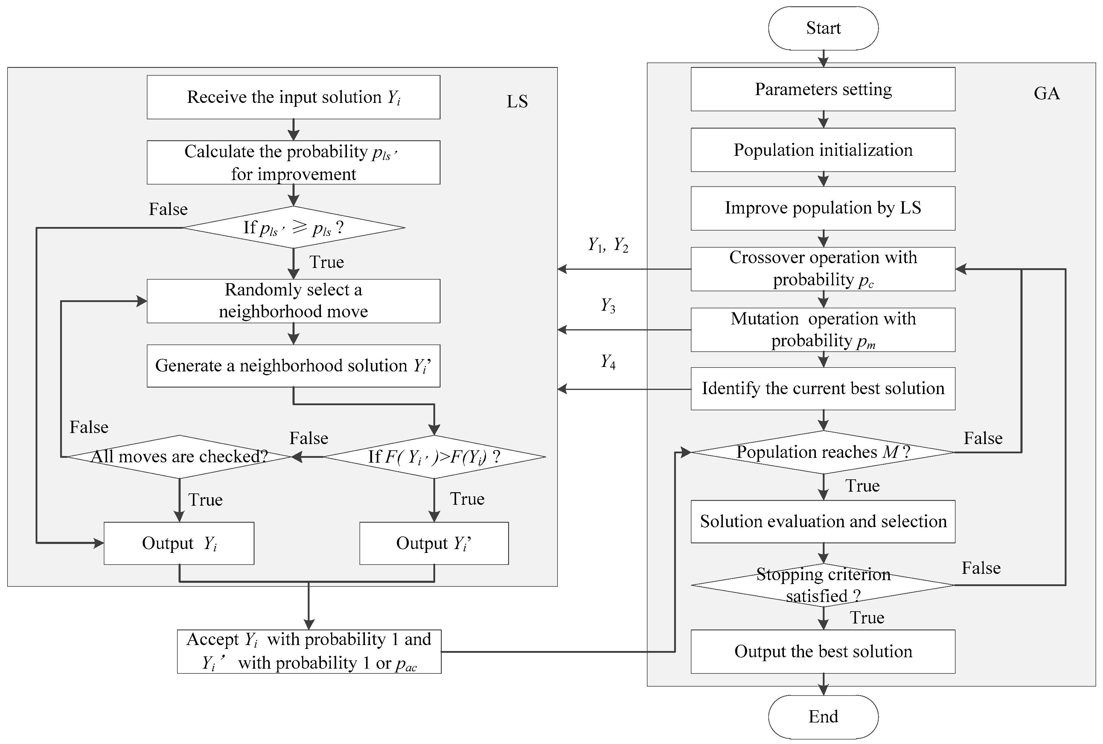
In this algorithm, GA-based operations are intended to guide the global evolution while LS is taken to find better local solutions both for the initial population and the new generated individuals during the evolution process. LS is also used to work as a post-optimization procedure in order to improve the best solutions in each iteration. The solution improved by LS is accepted with probability 1 when the solution is feasible; otherwise, the solution with probability pac is accepted. Additionally, a hybrid approach along with a two-phase solution generation heuristic is proposed to obtain high quality initial population; specific crossover and mutation operators are also proposed followed by a biased fitness function to evaluate the individuals. A high level overview of the presented HGALS is depicted below.
Step 1: Parameter setting: population size M0, maximum population M, crossover probability, mutation probability pm, infeasible solution accept probability pac, solution improve probability pls, terminate condition
Step 2: Taking solution generation and population initialization methods to obtain initial population P0
Step 3: Improve the population by LS
Step 4: Select individual X1 and X2 from the population following probability pc, conduct crossover operation to generate offspring Y1 and Y2, apply LS to improve Y1 and Y2 with probability pls, Y1 and Y2 are improved to be Y1′ and Y2′, accept Y1′ and Y2′ by probability 1 or pac
Step 5: Select individual X3 following probability pm to make new solution Y3 by mutation operation, apply LS to improve Y3 with probability pls, Y3 is improved to be Y3′, accept Y3′ by probability 1 or pac
Step 6: Improve the current best solution Y4 to be Y4′ by LS, accept Y4′ by probability 1 or pac
Step 7: If the population reaches M, evaluation individuals and select M0 solutions to make population P0, turn to step 3; otherwise, turn to step 8
Step 8: If the terminate condition is satisfied, turn to step 9; if not, turn to step 4
Step 9: Output the best solution.
The general structure of the presented HGALS is given in
Figure 2.
4.1. Solution Representation
For a GA-based heuristic, chromosome encoding strategy affects the performance of genetic operations [
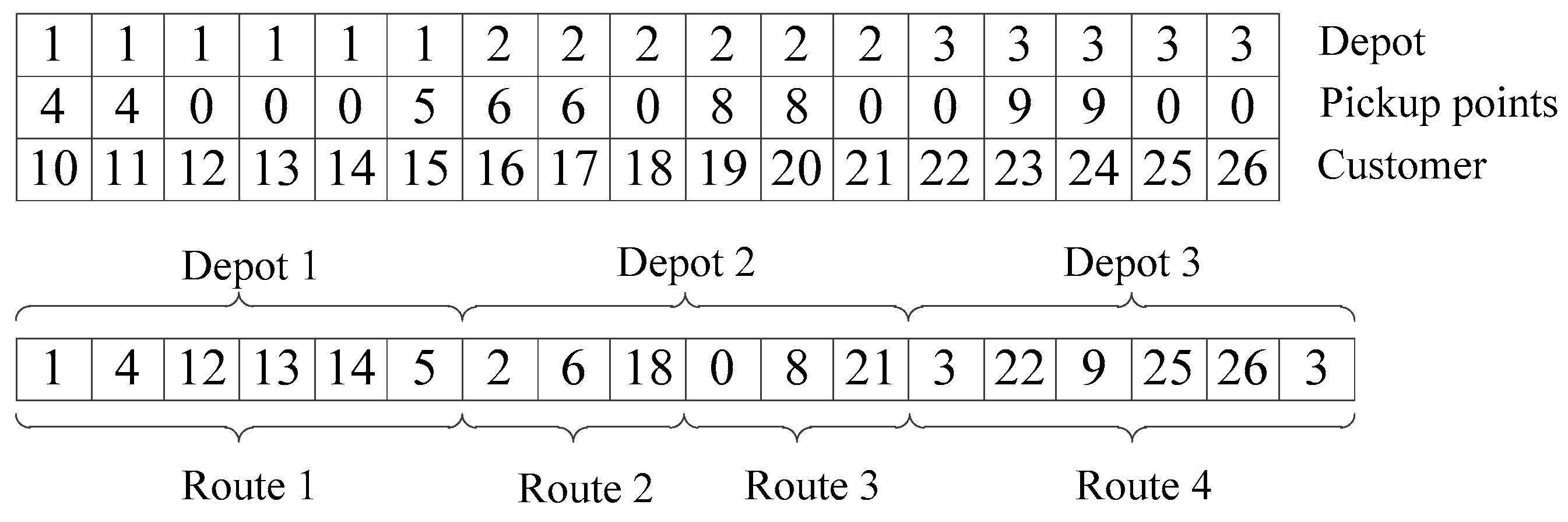
40]. Thus, the first and most crucial step in designing GA is to define an appropriate encoding scheme. According to the characteristics of the considered problem, a mixed encoding scheme is designed to represent a solution in which each chromosome includes two sections.
The first section is composed of three tiers of gene string with a fixed length of nc. The third tier is customer tier, which stores the customers. The second tier is used to index the service options information: if the value of a gene belongs to {nd + 1, …, nd + np}, it means that the corresponding customer in the third tier is served by CP and served by the pickup point. Otherwise, if the value of the gene is 0, it means that the customer is served by HD. The first tier is for depots and indicates the assignments between the depots and pickup points as well as depots and the customers with HD service.
The second section is to deal with the vehicle routing with a permutation of nd depots, np′ pickup points selected from NP, nc′ customers with HD service and a set of dummy zeros. Routes are started and ended at the same depots to serve the selected pickup points and customers with HD service one by one, zeros are used to terminate a route and start a new one in depots.
4.2. Solution and Population Initialization
As the quality of the initial solutions affects the final solution to a large extent, to obtain high quality initial solutions, we designed a two-phase heuristic named “Routing planning after the pickup points selection and services determination”. The procedure of the two-phase heuristic is depicted as follows:
Phase 1: Pickup points selection and service determination.
Step 1: Randomly select a pickup point combination set .
Step 2: Sort all the customers according to distance to the pickup points in , let be the number of the customers whose closest pickup point is p, and the corresponding customer set be .
Step 3: Select the pickup point p with the largest .
Step 4: If within the pickup point’s capacity, let the service option of its closest customer in be CP. Delete the customer in and . If p is in , delete it from and put it into .
Step 5: If , turn to step 2; otherwise, turn to step 3.
Step 6: If , turn to step 2; otherwise, turn to step 7.
Phase 2: Route planning
Step 7: Let be the node set that store the customers with HD service and selected pickup points in and whose closest depot is depot d. Rank all the nodes in with the increasing distance to the depots and put them into the corresponding sets.
Step 8: For each depot
and the nodes in
, the Traveling Salesman Problem (TSP) can be applied; the efficient algorithm proposed by Lin and Kernighan [
44] can be used for generating the TSP tour.
Step 9: Split the TSP tour by the method proposed by Prins [
45] without violating the vehicle capacity and working time constraints.
Step 10: Output the solution.
Based on the solution generation heuristic, the diverse population generation procedure is designed as follows:
Step 1: Randomly generate a non-redundant pickup point combination set with combinations, letting .
Step 2: Conduct the solution generation algorithm to generate solution S.
Step 3: If the selected pickup point in solution S already exists in P0, turn to step 1; otherwise, put S into P0.
Step 4: If the initial population size M0 is reached, turn to step 5; otherwise, turn to step 1.
Step 5: Terminate and output the initial population.
As can be seen by taking the solution and population initialization methods, solutions are different for selected pickup points and service options, each of which stands for a unique solution space, which will cover the whole solution space to the largest extent.
4.3. Fitness Function
To compare two individual factors, the evaluation function
F is defined as the sum of two components which are the objective function value and penalty cost, the evaluation function is formulated as follows:
where,
is the objective value of a solution;
,
,
,
and
stand for the amount that are beyond the constraints of the depot capacity, pickup point capacity, available vehicles, vehicle capacity and working time respectively;
,
,
,
and
are the corresponding constant parameters that reflect the degree of the penalty.
4.4. Individual Evolution and Selection
In population-based heuristics, one of the greatest advantages is search parallel in wide solution space, rendering population diversity an important factor that affects the performance. Current widely used objective function-based individual evolution may shrink the search space and lead to premature convergence. In this study, we revise the biased fitness function proposed by Vidal et al. [
46]. In this method, the objective value of a solution and its contribution to population diversity are jointly considered.
For an individual
I, letting its
nclose closest neighbors be stored in set
Nclose, the diversity contribution of individual
I to the population in
Nclose is defined as the average distance to the individuals in
Nclose computed by Formula (21). A normalized Hamming distance based on pickup points’ status, customers’ service options and the assignments of two individuals is adopted to show the difference between solutions. The distance is computed according to Formula (22).
where,
sci(
I) stands for the assignment of customers with HD service,
spi(
I) stands for the assignment of pickup facilities and
pci(
I) stands for the assignment of customers with CP service
. γ
1, γ
2 and γ
3 are the coefficients of the three factors, γ
1 + γ
2 + γ
3 = 1.
Let
r(
I) be the rank of individual
I in a subpopulation with respect to
F and the biased fitness function is given by Formula (23).
It can be seen that, for each subpopulation with nclose customers, when solutions are selected by elitist strategy, excellent solutions can be protected as well as the diversity achieved.
4.5. Crossover Operation
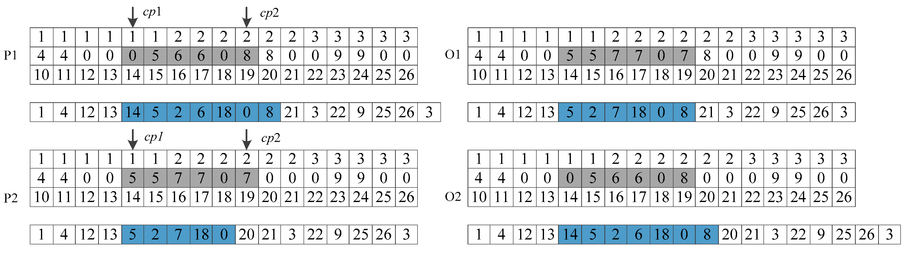
Crossover operation aims to generate offspring by mimicking mating between parents and exchanging gene information in the hope that children will obtain the best parts of their parents, as well as diversify the search. Due to the fact that the genes and length of chromosomes vary in solutions, a modified two-point crossover is introduced, which is depicted in
Figure 4. This crossover operation is conducted by exchanging the middle part of the second tier of the first section of the selected two parents between the two selected crossover positions. The process is described as follows:
Step 1: Randomly select a pair of parents P1 and P2 by probability pc from the population.
Step 2: Uniformly select two positions from [1, nc], letting the smaller one be cp1 and the other cp2.
Step 3: For each gene in position [cp1, cp2], exchange the middle part of the second tier of the first part of the two chromosomes.
Step 4: Adjust the second sections of the two chromosomes according to the mapping relationship.
By taking this crossover operation, new solutions are generated by exploring new statuses of pickup points, customers’ service options as well as the routes.
4.6. Mutation Operation
Mutation operation takes place immediately after the crossover operation, which may help GA jump out of the local optima by finding uncovered solution spaces [
47]. In our research, we take gene-based mutation, which is conducted on the second section of a chromosome, in the following process:
Step 1: Select a solution P3 according to probability pm.
Step 2: Randomly select a mutation position cp3 from 1 to L(P3), where L(P3) is the length of the second section of the chromosome.
Step 3: Identify the type of the selected gene; conduct the following two cases equally.
Case 1: If it is a pickup point, each of the three operators is selected randomly:
Operator 1: Close this pickup point.
Operator 2: Exchange the assigned customers with the closest pickup point if it is open.
Operator 3: Close it and open a randomly selected one which is not in the current solution.
Case 2: If the gene is a customer or zero, remove it and insert it into a randomly selected position between 1 and L(P3).
It can be seen that, in this crossover, the operation can be performed on all search spaces by changing the status of pickup points, customers’ service options as well as the routes.
4.7. Local Search
Local search aims to improve the new generated solutions during the evolution process within a few modifications. As the neighborhood defines the way to produce a new solution, the most important issue when designing a local search is to identify effective neighborhood structure [
40]. For the customers’ service options and vehicle routing in our problem, we design two kinds of neighborhood structures for service option and vehicle routing respectively.
For the service option neighborhood structure, two moves are included: they are HD to CP and CP to HD move, namely N1 and N2. More precisely, for N1, we randomly select a customer served by HD and identify its closest pickup point. If the pickup point is already selected, let the customer be served by it; otherwise, open the pickup point and serve the customer. For N2, we randomly select a pickup point and release one randomly selected customer and let him or her be served by HD.
When it comes to routing neighborhood structure, we take the nine route neighborhood moves proposed by Prins [
45] which can comprehensively search the routing space.
Let
stand for the trip visiting vertex
u,
x and
y which are the successor of
u and
v in their respective trips. Define the neighborhood of vertex
u as the
closest vertices, where
is a granular threshold restricting the search to nearby vertices [
48]. The following moves are concluded:
N3: If u is a customer or pickup point, remove u then insert it after v;
N4: If u is a customer or pickup point and x is a customer or dummy zero, remove them then insert after v;
N5: If u is a customer or pickup point and x is a customer or dummy zero, remove them then insert after v;
N6: If u and v are customers or pickup points, swap u and v;
N7: If u and v are customers or pickup points, and x is a customer or dummy zero, swap and v;
N8: If u and v are customers, x and y are customers of dummy zeros, swap and ;
N9: If , replace and by and ;
N10: If , replace and by and ;
N11: If , replace and by and .
N3 to N5 correspond to insertions, whereas N6 to N8 are swaps. The aforementioned six moves can be worked on both the intra-route and inter-route. N9 is an intra-route 2-opt, while N10 and N11 are inter-route 2-opt. It can be seen that, compared to the initial moves in Prins [
45], zeros are also used to formulate new neighborhood solutions, which may help to explore the search space.
When applying LS procedure, the above neighborhood moves are selected randomly to generate a new solution. The procedure terminates when either an improved solution is obtained or all neighborhood moves are checked without finding a better solution. The structure of LS can be seen in
Figure 2.
4.8. Computational Complexity Analysis
Letting the scale of the considered problem be
,
Imax is the maximum iteration. In the presented algorithm, the computational complexity for population initialization is
. In each iteration, the computational complexity for decoding, crossover operation, mutation, evaluation and local search are
,
,
,
and
, respectively. The computational complexity of the whole algorithm can be calculated as:
As can be seen from Formula (24), the presented method belongs to polynomial algorithm and can be solved in polynomial time. More specifically, the computational complexity of the algorithm increases with the iterations and is proportional to np and (2ns+nc)2.
5. Computational Experiments
In this section, we perform numerical experiments to evaluate the overall performance of the proposed model and method. We first provide the implementation details of HGALS for the parameters setting. As the proposed problem belongs to a variant of LRP, the performance of the HGALS in solving LRP is then evaluated based on benchmark instances. Subsequently, a real-world instance is taken to analyze the effects of simultaneous HD and CP on the Last Mile distribution system. Finally, the validity of the presented method in solving the proposed problem is verified based on generated instances. All algorithms are coded in C language and compiled on Visual Studio 2013, implemented on a PC with an Intel Core Duo CPU at 1.74 GHz and 4GB memory under Window XP system.
5.1. Parameters Setting
To find suitable parameters, extensive experiments are conducted based on the generated instances depicted in
Section 5.4. For GA-based heuristics, the most important parameter is the population size; with bigger
M0, excellent solutions will be improved with much smaller probability, and it will take longer to find better solutions. Conversely, the population cannot sample the solution space which may lead to premature convergence. During the tests, since we found that the suitable initial population is closely related to
np and variable population strategy helps a lot, it was finally decided as
M0 = 4
np and
M = 2
M0. According to the decided
M0 and
M,
pc,
pm,
pls and
pac are selected to be 0.45, 0.25, 1.0 and 0.25 respectively. Other parameters:
h = 0.2, α
1 = 1000, α
2 = 200, α
3 = 100, α
4 = α
5 = 10, γ
1 = γ
3 = 0.3, γ
2 = 0.4.
5.2. Tests Based on Benchmark Instance
To show that the presented method is suitable to solve LRP, the benchmark instances proposed by Prins et al. [
49] are used, which can be found at
http://prodhonc.free.fr/Instances/instances_us.htm. The designed operators for pickup points are performed on the depots both for the solution initialization and mutation. For the terminate condition, we take the maximum iterations without improving the best solution. The specific value depends on instance size: it is 200 for small-sized instances (
n ≤ 50), 400 for mid-sized instances (50 <
n ≤ 100) and 600 for large-sized instances (
n > 100). During the tests, each instance was independently run 10 times; the results obtained by the presented heuristic are provided in
Table 2. For the notions used in the table, LB stands for the best known lower bound, BKR stands for the best known result, CPU stands for the average running time in seconds and Gap/BKR stands for the gap to BKR.
From
Table 2, we can see that all the instances are solved with an overall average runtime of 277.2 s. Average gap to the best-known solution is 0.47%. For all instances containing 50 or less customers, the presented method is successful at finding almost all the optimal solutions. Moreover, for the instances with 100 and 200 customers, the average gap to the best-known solution is not changed dramatically.
Moreover, considering the most recent and effective methods in the literature, the performance comparison is provided in
Table 3 based on the CPU and Best Gap/BKR. The compared algorithms are GRASP in Prins et al. [
49], MAPM in Prins et al. [
39], LRGTS in Prins et al. [
50], GRASP+ELS in Duhamel et al. [
36], SALRP in Vincent et al. [
35], ALNS in reference [
51], MACO in [
32], GRASP+ILP in Contardo et al. [
52], GVTNS in Escobar et al. [
38] and Hybrid GA in Lopes et al. [
43].
Among those compared algorithms, GRASP+ILP is on average the most effective on this set of benchmark instances followed by ALNS, GVTNS, MACO and SALRP. Our algorithm obtains similar results with SALRP and performs much better than GRASP, MAPM, LRGTS and GRASP+ELS. As CPU times depend on many factors (such as computers and programming languages used) [
43], the proposed method seems faster than SALRP, ALNS and GRASP+ILP.
The computational results show that our algorithm can effectively solve the instances and is applicable to LRP.
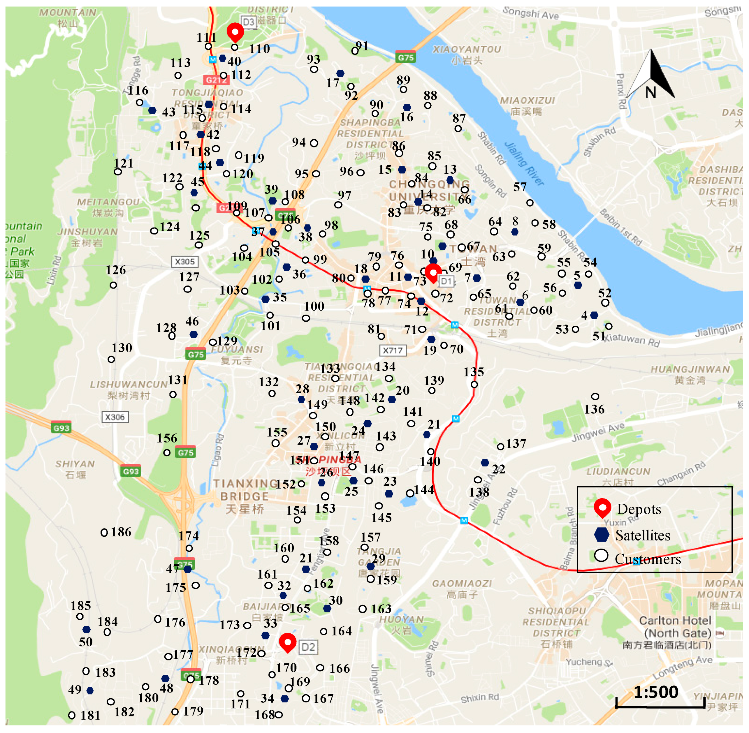
5.3. Real-World Instance
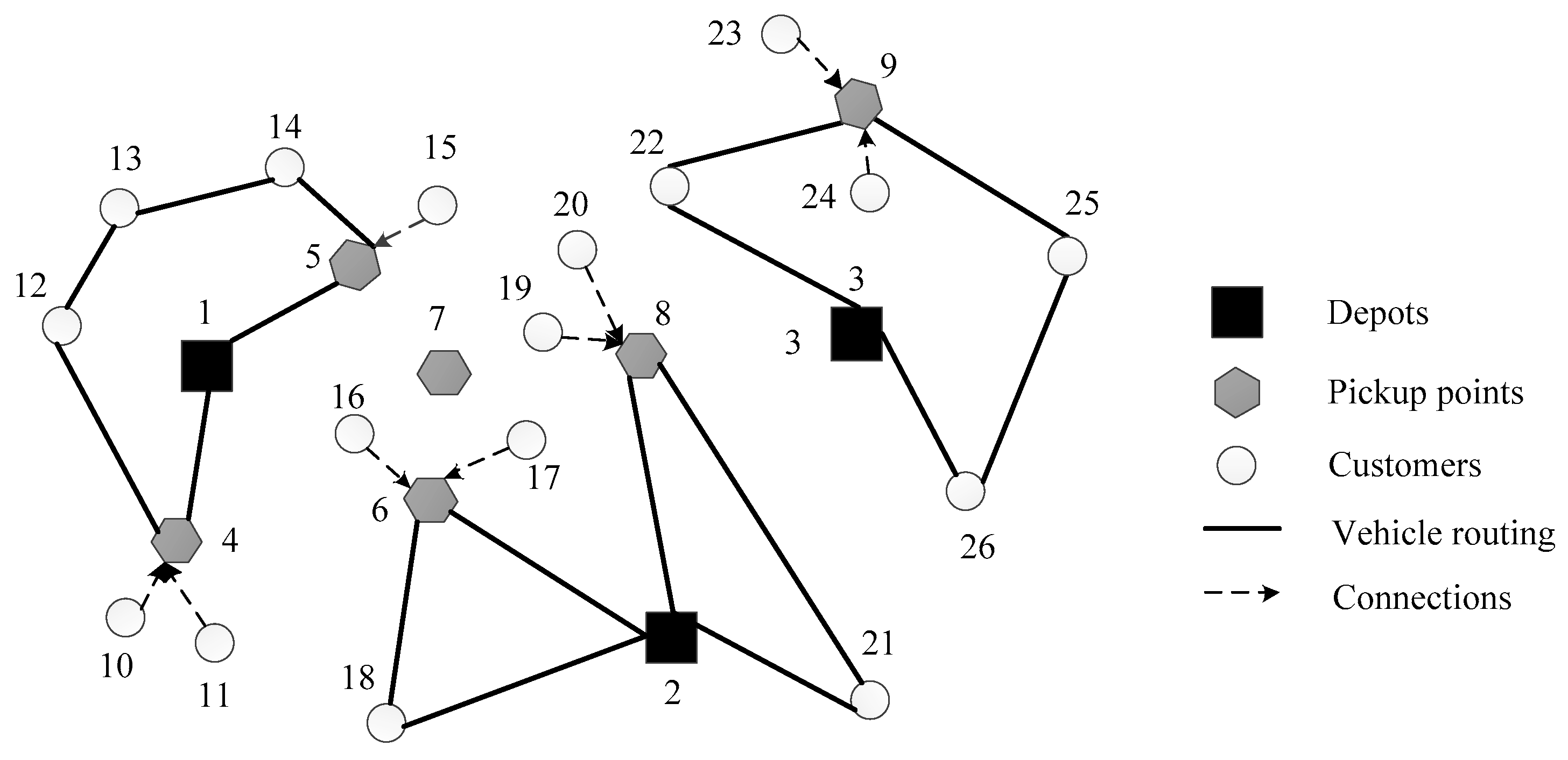
This section presents the test based on a real-world Last Mile distribution system of Shapingba District in Chongqing city. The network consists of three depots (numbered from 1 to 3), 47 candidate pickup points (with number from 4 to 50) and 136 customers (with numbers from 51 to 186). The locations of these nodes are shown in
Figure 5. Other main parameters are given as follows:
Dpc = 600 m,
uH = 1.5 min,
uP = 10 min,
pH = 10%,
μsd = 1.5. For the algorithm terminate conditions, to get a better solution, we take the maximum iterations
Imax and
Tmax into consideration simultaneously; three terminate conditions are considered according to the instance scales: (
Imax,
Tmax) = (1 × 10
4, 600 s), (2 × 10
4, 900 s), (3 × 10
4, 1200 s). After running the algorithm, the obtained pickup point locations and customer assignments are reported in
Table 4, and the vehicle routing information is given in
Table 5.
To show the advantages of the proposed model, we now report the comparison of the proposed model with the scenario of only HD service, which can be seen in
Table 6.
From the comparison, it can be clearly seen that although added pickup points cost by providing CP service, the total cost is reduced by 1050 and accounts for 17.6%. When analyzing the reason, we find that the vehicles are largely reduced by providing HD and CP services simultaneously, which saved the fixed vehicle cost and routing cost accordingly. Besides, the increased customers served by CP reduced the second delivery cost. These two factors work together, reducing the cost to a large extent.
In this research, we take the routing cost cij by dij multiplying the unit routing cost. From the comparison of the total routing cost of the two scenarios, we can deduce that the travelling distance is reduced by 33%. As the carbon emission is closely related to the travelling distance, the proposed model can help to reduce the carbon emission effectively.
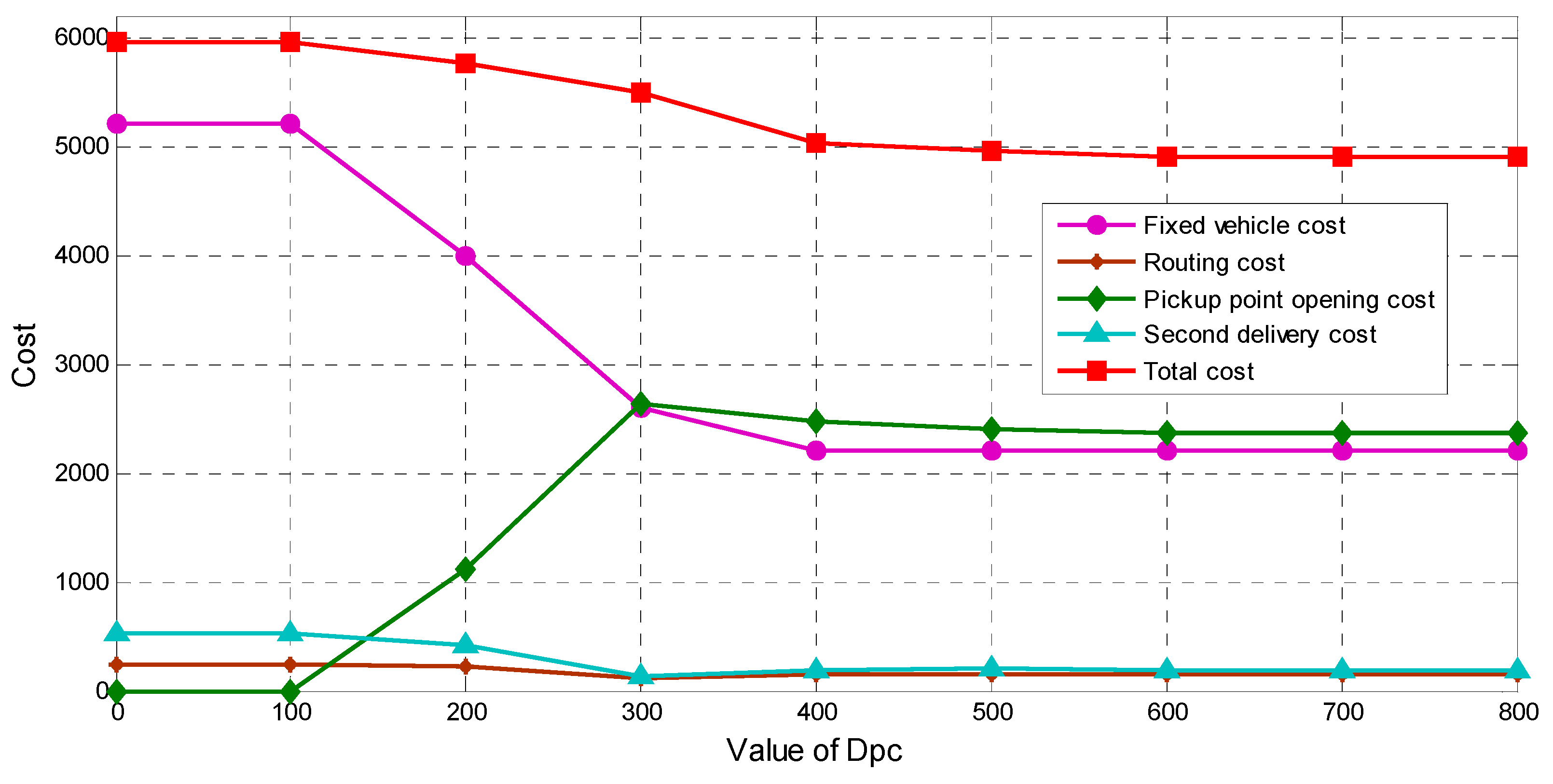
As CP service provides an important role in reducing the operation cost, to have more insights, we conduct a sensitive analysis to show how the acceptable distance
Dpc influences the cost. When
Dpc ranges from 100 to 800 with step 100, the results are reported in
Table 7 and
Figure 6. It is worth mentioning that the scenario when
Dpc = 0 is with only HD service.
From the sensitive analysis, we can see that when Dpc ≤ 100 m, the results obtained are the same with the only-HD scenario, which indicates that when Dpc ≤ 100 m, CP service shows no advantages when compared to HD and there is no need to provide CP service. When 100 < Dpc ≤ 600 m, there comes a continuous fall of the total cost, which means that with the distance increasing, better solutions are obtained due to the provided CP service. After that, the results stay unchanged which is constrained by the closest customers and the capacity of pickup points. From a cost optimization perspective, Dpc = 600 m is the most acceptable distance when designing the Last Mile distribution system in this instance.
Thus, we can draw the conclusion that, within appropriate acceptable distance Dpc, simultaneous HD and CP are effective at reducing the cost within a wide range of Dpc, and a suitable distance exists for each Last Mile distribution system.
5.4. Algorithm Components Performance Analysis
In this section, a computational study is carried out to compare our approach with standard GA&LS (SGALS) to show the effectiveness of the designed algorithm components in solving this problem. In the SGALS, random solution generation, objective function-based individual evaluation and classical single point crossover and mutation on the second tier of the chromosome are considered.
We first generate a set of different scales of instances based on the real-world instance parameters. For the instances, the number of depots, pickup points and customers range from 2 to 12, 10 to 30 and 50 to 200, respectively. The instances are presented as “I<depot number>-<pickup point number>-<customer number>”. The instances are generated as follows: depots and pickup points are randomly decided within the area with a radius of 15 km to reflect the relationship between the customers and pickup points; customers are randomly assigned within a radius of 1 km of selected pickup points; the capacity of depots as well as the vehicles are assigned with the requirement that all customers could be served; the capacity of pickup points are random value in [100, 120, 150, 180, 200] and the opening costs are [60, 80, 100, 120, 150] accordingly; customers’ demands are random value in [15, 20, 25, 30, 35]. Other parameters are the same to the real-world instance in
Section 5.3. The two algorithms are run ten times independently for each instance; the results are reported in
Table 8.
From
Table 8 we can observe that our approach can always obtain the best solutions and run faster than SGALS. The results clearly indicate that the proposed components which constitute the algorithm are necessary and useful to enhance the performance both in the search ability and the stability when comparing the results obtained by SGALS. This can be seen by the improvement of 1.83% in Best Gap and 4.27% (7%–2.73%) in Average Gap. We can also draw the conclusion that the LRPSHC is very complex since the SGASA can obtain the same best solution as HGALS only for instance I2-18-80.


