Game Theoretic Analysis of Pricing and Cooperative Advertising in a Reverse Supply Chain for Unwanted Medications in Households

Abstract

Improper disposal of household unwanted medications (UMs) is an emergency problem around the world that adversely affects the sustainability of the environment and human’s health. However, the current disposal practices, mainly based on advertising and collecting status, are unsatisfactory in most countries and regions. Thus, some scholars proposed an alternative disposal practice that is to provide incentives to customers. This study aims to compare a Single Model (advertising only) with a Joint Model (advertising with take-back pricing) in a two-echelon reverse supply chain (RSC) that is composed of one disposer and one collector. In each model, four games (non-cooperative, collector as the Stackelberg leader, disposer as the Stackelberg leader, and cooperative) were established in order to identify the optimal pricing and advertising strategies for both members. The results of the study indicate that there is a Pareto dominant range for Joint Model compared to Single Model, whereas Single Model has no Pareto improvement in any games. Furthermore, in non-cooperative games of Joint Model, it is better to implement the leader-follower structure rather than simultaneous movement structure. Additionally, it is verified that the cooperative game is feasible, which leads to the cooperation between the disposer and the collector, and the extra profit from the cooperation can be shared based on the Nash bargaining game. However, in Single Model, it is better for the disposer to act as a channel leader and the collector figures the follower.

1. Introduction

Over the past decade, pharmaceutical expenditure and consumption have increased continuously as a result of population aging, the rising prevalence of chronic diseases, new treatment opportunities, and so forth [1]. In addition, more spare medications are stored up for any contingency [2]. However, these medications may not be consumed entirely, owing to expiry, condition resolved or symptoms improved, side effects or other reasons [3], resulting in a universal issue of massively unwanted medications (UMs) accumulating in households around the world.

UMs include expired, unused, spilled and contaminated pharmaceutical products, drugs, vaccines, and sera that are no longer required and need to be disposed of appropriately [4]. Improper disposal of UMs can cause damage to human health (deterioration due to expiry or taken by anyone other than the prescribed patient) and the environment [5,6,7,8], especially to the aquatic ecosystems [9,10,11]. Moreover, UMs may be repackaged and resold to the market illegally [7], which constitutes a grave threat to public safety. Accelerative concern has been given to UMs and their proper disposal.

Although the European Union (EU) has a directive statement that member states are obligated to ensure appropriate collection systems are in place for unused or expired medicinal products [12,13], this code is applied inconsistently and seems to be unenforced [2]. Numerous studies suggested that the sustainable environmentally appropriate method to dispose of UMs is to return them to the pharmacy [2] or take-back locations [14]. Nonetheless, households’ most common method for disposal of pharmaceuticals is still by garbage and sewage in many countries including the United Kingdom [5], the United States [3,15], Kuwait [16], Lebanon [7], Saudi Arabia [17], and Serbia [18]. Furthermore, in some regions where pharmacies offer the service of collecting UMs, the evaluated effectiveness has a number of weaknesses [19].

There exists some literature on the performance of reverse supply chains (RSCs). For instance, Yoon and Jeong [20] focused on implementing coordinative contracts between manufacturers and retailers in the RSC so as to maximize the total performance. With respect to general RSCs, the RSC for UMs is rather challenging and tough to implement. Xie and Breen [21] explained that the reasons were lack of commercial motivation and legislative enforcement for actors to return or collect UMs and requirement for more investment, which is not cost-effective. Thus, researchers paid less attention to RSCs for UMs.

Commercially, advertising can largely promote sales. Different cooperative advertising models have been studied more sufficiently in the forward supply chain (FSC) [22,23,24,25,26,27,28,29,30,31,32] including two excellent reviews [22,23]. On the other hand, advertising occupies a crucial position in promoting the quantity of collected used products [33]. It is because better collection efficiency required end-users’ consciousness [34] and advertising can raise public awareness about the environment by highlighting the environmental risk associated with inappropriately disposed of Ums [35]. However, few articles have investigated the role of advertising in the RSCs for UMs. Although Hong et al. [33] have investigated the optimal decisions of cooperative advertising in closed-loop supply chains that considered the retailer’s local advertising expenditure, it is not suitable for studying the collection of UMs. Thus, different from previous research, this paper firstly supposes a model where the quantity of collected UMs is influenced by channel parties’ advertising expenses in the RSCs (referred to as Single Model).

To improve the situation of UMs holders’ deficiency to return, Huang et al. [36] and Weraikat et al. [37] suggested providing incentives to customers. Huang et al. [36] established a tri-level programming model for recycling logistics networks in which the government undertook responsibility and related cost for recycling and getting rid of expired medications. In this research, UMs are eliminated as garbage and have no salvage value. Weraikat et al. [37] proposed a two-echelon pharmaceutical RSC with two coordination models, which are Producer-customer scheme and Producer-customer-3PL scheme. They provided incentives to stimulate customers to return UMs before their shelf life was up. Different from Huang et al. [36], this study classified UMs according to their shelf life and recycled reusable ones for more profit. However, they both seem to leave out of consideration of a crucial marketing tool, advertising. In view of this point, this research considers providing the customers with a take-back price incentive that is similar to the works of Huang et al. [36] and Weraikat et al. [37]. Furthermore, advertising is taken into account from collectors who are facing customers and can take UMs back conveniently and easily. Hence, this study refers to cooperative advertising to jointly promote the UMS take-back quantity that is rarely considered in existing research on RSCs. Thus, this paper secondly supposes a model where the quantity of collected UMs is influenced by both take-back price and channel parties’ advertising expenses in the RSCs (referred to as Joint Model).

To this end, this paper proposes a two-echelon RSC composed of one disposer and one collector. It is assumed that advertising is indispensable while the RSC can choose whether to deploy a take-back price incentive. There is a threefold consideration for this assumption. First, if there does not exist publicity and advertising, the information of collection activities cannot spread out and nobody would join in. Second, advertising is a kind of education investment to improve the awareness of the environment and medication safety. Third, in real cases, the vast majority of collecting activities do not provide a take-back price incentive. Therefore, two models as mentioned before are developed: (i) take-back pricing and advertising jointly impact to the quantity of collecting UMs (Joint Model); (ii) the quantity is influenced only by advertising (Single Model).

Within the research of cooperative advertising composed of a manufacturer and a retailer, Yue et al. [24] and Wei and Xie [28] investigated two game models including Stackelberg-manufacturer and cooperative game. Meanwhile, considering retailers’ increasing power in supply chains, another two games, Stackelberg-retailer and equal power as in Nash game, were taken into account [26,27,29,31]. As for the issue of UMs collection, the deficiency or ambiguity of related laws and regulations in most countries and regions results in the uncertainty surrounding who should take the responsibility to collect UMs. Thus, there exist different collection parties from organizers to executors with diverse channel power. Hence, in each model, four types of disposer-collector relationship are considered: non-cooperative, disposer as Stackelberg leader, collector as Stackelberg leader, and cooperative game models. The reason why we propose a RSC instead of a closed-loop supply chain is that UMs are useless and cannot be remanufactured, resulting in no close relationship with the FSC. This study focuses on the following decision-making problems:

(1)

On which condition the RSC could and would like to use a take-back price incentive;

(2)

how to choose best RSC structure under different situations;

(3)

how to effectively allocate the fund between pricing and national and local advertising;

(4)

and wether one party would like to share another’s advertising expense?

This paper is structured as follows. In Section 2, the basic problems and assumptions in the two models are described, followed by analyzing the models in Section 3. Then, comparisons and discussions of the two models and numerical examples are made in Section 4. Finally, in Section 5, the main results are concluded with suggestions for future research.

2. Problem Description and Assumptions

This paper focuses on a two-echelon RSC composed of a single collector and a single disposer, since UMs collection activity lacks competition for less monetary benefit from collecting expired medications (except the illegal business which collects and repackages expired medications then sells them to suburbs or villages) and are generally formed by the driving force of related law and regulation, social responsibility, and resell reusable unexpired medications. From practical perspectives, the original price and categories of medications are ignored for their uselessness to patients. The responsibility of the collector is to collect and make a preliminary classification of UMs and the disposer takes all the collected UMs from the collector and disposes of them, such as incinerating medicine waste, recycling glass and packages, repacking reused medications, and so on. The collector can be a pharmacy, community, third-party logistics provider, etc., who faces UMs holders and can take them back conveniently and easily. The disposer can be played by the pharmaceutical company, government, and specialized agency. The common disposer-collector combinations are pharmaceutical company-pharmacy [37,38], government-pharmacy (most European countries) and government-community (some states in America).

In addition, two models are designed with and without an incentive by offering customers take-back price. In Section 4, this paper will compare and analyze the results of the two models and the suitable conditions for potential application.

The symbols are explained in

Table 1. Definition of symbols.

Parameters
$\beta$	Customers’ sensitivity coefficient to the collector’s take-back price
$\alpha$	Potential take-back scale
$s_d$	Disposer’s unit revenue incurred by disposal activity
$s_c$	Collector’s unit revenue incurred by collection activity
$K_c$	Effectiveness of collector’s local advertising
$K_d$	Effectiveness of disposer’s national advertising
$k$	Advertising ratio (i.e., $K_d/K_c$)
Variables
$p_c$	Collector’s take-back price
$p_d$	Disposer’s price claimed for collector
$m$	Collector margin (i.e., $m=p_d+s_c-p_c$)
$n$	Disposer margin (i.e., $n=s_d-p_d$)
$a$	Collector’s local advertising expenditure
$A$	Disposer’s national advertising investment
$t$	Advertising participation rate
$\pi$	Profit

and proposed models are based on the following assumptions. Disposer’s unit revenue $s_d$ and collector’s unit revenue $s_c$ are set as constants that are in connection with the parties’ own characteristics. More specifically, if the disposer is a government who regards improper disposal of medications as of special importance that will cause a huge reduction of its utility for the damage to resident and environment, the disposer will make more policies (e.g., toll tax for pharmaceutical industry and more collection subsidy) to support collection activities, then $s_d$ increases. When a manufacturer acts as the disposer, $s_d$ can be derived from a corporate sense of responsibility, actual monetary profit from resale or donation of reusable medications or the benefit from avoiding being punished in an existing related law. Likewise, when the collector is a pharmacy, $s_c$ may be generated from the benefit of growing sales by collecting activity or sense of responsibility. Here, it needs to be explained that $s_d$ and $s_c$ are NET values, in which the related cost has been deducted. This treatment does not affect models. $t$ denotes the fraction of collector’s advertising expenditure, which is the percentage of the disposer agreeing to share with the collector. Therefore, $0\le t\le 1$.

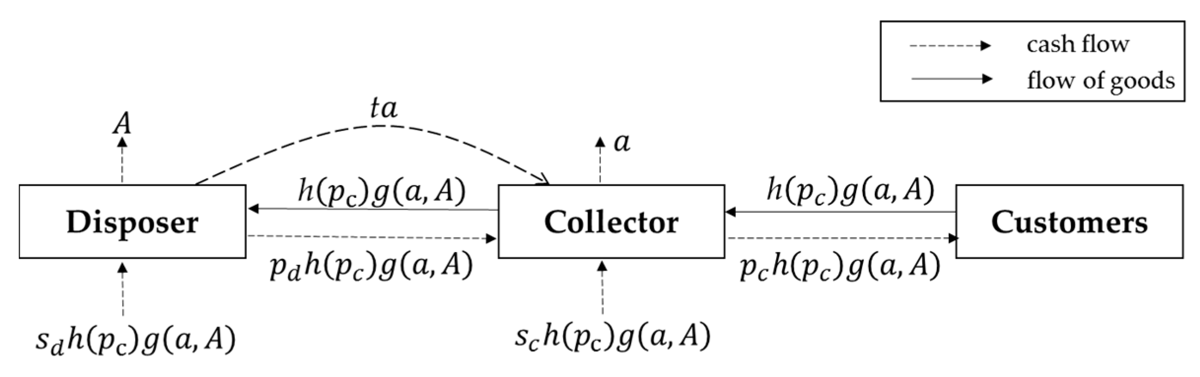
2.1. Disposer-Collector RSC with an Incentive of Take-Back Price

Model with a take-back price incentive (Joint Model) is illustrated in Figure 1. For more quantity of collected UMs and profit, the collector offers a take-back price to customers and both disposer and collector make advertising expenses. Throughout this study, the mass of collected UMs is stated as quantity, however, the model can be adjusted according to the actual situation. For instance, the UMs can be collected according to weight. Accordingly, all the corresponding parameters should be tied to weight.

There are vertical cooperative advertising strategies that the disposer shares part of the collector’s advertising expenditure. Decision variables for the disposer are national advertising investment, the price given to the collector and the cooperative advertising compensation. The collector’s decision variables are advertising expenditure and the take-back price.

In view of the situation that the quantity of collected UMs is influenced by the take-back price and advertising, the take-back quantity $Q\left(p_c,a,A\right)$ depends on the take-back price $p_c$ and the advertising levels $a$ and $A$ as $Q\left(p_c,a,A\right)=h\left(p_c\right)g\left(a,A\right)$, which means that the quantity is jointly affected by price-related function $h\left(p_c\right)$ and advertising-related function $g\left(a,A\right)$. A simple price model is assumed to express the positive effect of the take-back price on the collection quantity,

$$h\left(p_c\right)=\alpha +\beta p_c$$

(1)

$h\left(p_c\right)$ increases with respect to $p_c$. The two parameters $\alpha$ and $\beta$ are positive and can be interpreted as a potential take-back scale without any incentive from price and advertising and price sensitivity of customers. $Q(p_c,a,A)=h(p_c)g(a,A)=\left(\alpha +\beta p_c\right)g\left(a,A\right)=\alpha g\left(a,A\right)+\beta g{\left(a,A\right)}^{}{p}_c$. It can be seen that advertising has two effects in promoting customers’ environmental awareness and sense of responsibility, where the front part of the formula expresses that advertising could increase the voluntary quantity and the latter partial indicates that advertising makes the customers more sensitive to the take-back price. $g\left(a,A\right)$ is the function proposed by Xie and Wei [28]. That is $h\left(a,A\right)=K_c\sqrt{a}+K_d\sqrt{A}$. The square root advertising demand function indicates a diminishing marginal demand for increasing advertising expenditure and is further used by SeyedEsfahani and Biazaran [29] and Aust and Buscher [31]. $a$ and $A$ denote local and advertising expenses and the two parameters $K_c$ and $K_d$ are positive constants and can be interpreted as the effectiveness of the collector’s and the disposer’s advertising. According to Aust and Buscher [31], the collector’s net profit margin $m$ is brought into the equation as a new decision variable,

$$m=p_d+s_c-p_c$$

(2)

Hence, the following modified price-related and advertising-related functions are derived.

$$h\left(p_d,m\right)=\alpha +\beta \left(p_d+s_c-m\right)$$

(3)

$$g\left(a,A\right)=K_c\sqrt{a}+K_d\sqrt{A}$$

(4)

For the sake of simplicity, denote

$$\overline{\alpha }=\alpha +\beta s_c$$

(5)

Thus,

$$h\left(p_d,m\right)=\alpha +\beta \left(p_d+s_c-m\right)=\overline{\alpha }+\beta \left(p_d-m\right)$$

(6)

The subscripts “$d$”, “$c$”, and “$d+c$” represent parameters related to the disposer, the collector, and the whole system. The profits of disposer ${\pi }_d$, the collector ${\pi }_c$, and the entire system ${\pi }_{d+c}$ can be written as follows respectively.

$${\pi }_d=\left(s_d-p_d\right)\left[\overline{\alpha }+\beta \left(p_d-m\right)\right]\left(K_c\sqrt{a}+K_d\sqrt{A}\right)-A-ta$$

(7)

$${\pi }_c=m\left[\overline{\alpha }+\beta \left(p_d-m\right)\right]\left(K_c\sqrt{a}+K_d\sqrt{A}\right)-\left(1-t\right)a$$

(8)

$${\pi }_{d+c}=\left(s_d+s_c-p_c\right)\left(\overline{\alpha }+\beta p_c\right)\left(K_c\sqrt{a}+K_d\sqrt{A}\right)-a-A$$

(9)

Note that, in this model, $s_c$ and $s_d$ can be less than 0 when the cost caused by the activity exceeds the revenue. However, they cannot be less than 0 simultaneously for the non-negativity of the system’s profit, which should guarantee $s_d+s_c-p_c>0$. Profits of the disposer and the collector should be nonnegative, which implies $n=s_d-p_d>0$ and $m=p_d+s_c-p_c>0$.

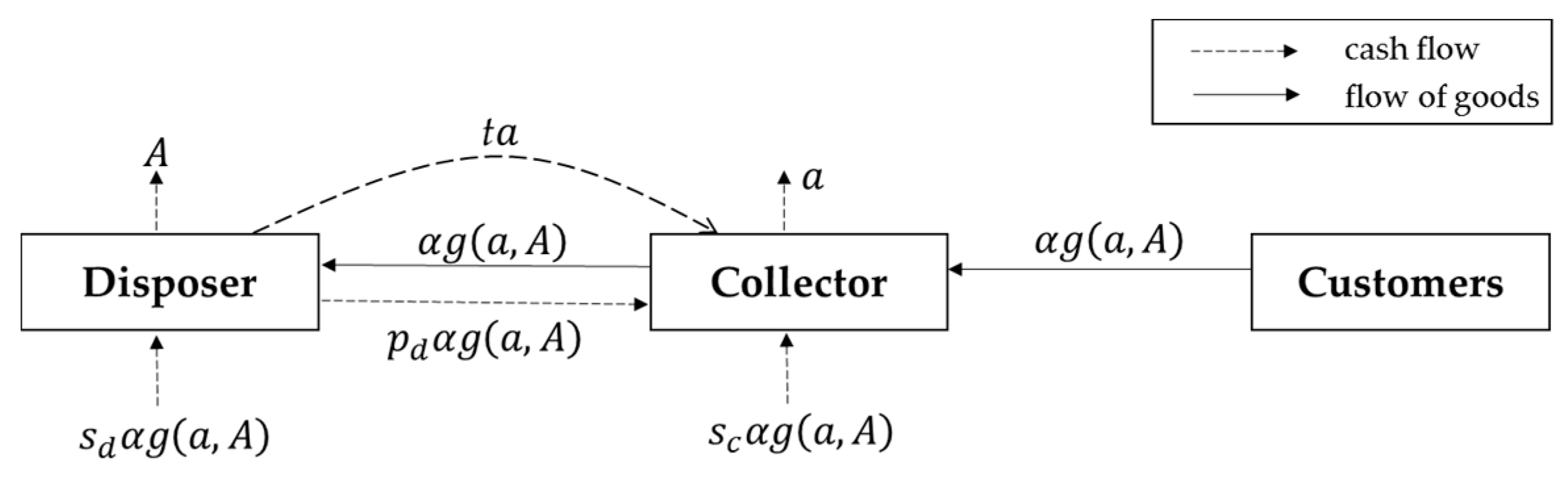
2.2. Disposer-Collector RSC without an Incentive of Take-Back Price

Another model without regard to customer incentive (Single Model) is presented in Figure 2. The collector takes no account of take-back price to promote quantity of collected Ums, which is solely affected by two members’ advertising expenses.

Regardless of the take-back price paid to the customers, the quantity of collected UMs is just a function of the collector’s local advertising expenditure $a$ and disposer’s national advertising investment $A$, which is

$$Q\left(a,A\right)=\alpha \left(K_c\sqrt{a}+K_d\sqrt{A}\right)$$

(10)

Then, the functions of the disposer’s profit ${\pi }_d$, the collector’s profit ${\pi }_c$ and the profit of whole supply chain ${\pi }_{d+c}$ are as follows.

$${\pi }_d=\left(s_d-p_d\right)\alpha \left(K_c\sqrt{a}+K_d\sqrt{A}\right)-A-ta$$

(11)

$${\pi }_c=\left(p_d+s_c\right)\alpha \left(K_c\sqrt{a}+K_d\sqrt{A}\right)-\left(1-t\right)a$$

(12)

$${\pi }_{d+c}=\left(s_d+s_c\right)\alpha \left(K_c\sqrt{a}+K_d\sqrt{A}\right)-A-a$$

(13)

3. Models

3.1. Four Games of Disposer-Collector Relationship with Customer Incentive

3.1.1. The Non-Cooperative Nash Game

This model is based on the situation that the disposer and the collector have a symmetrical distribution of power. The situation can be modeled through the Nash equilibrium, where both members make decisions concurrently and non-cooperatively to maximize their own profit. Hence, the decision problems of the disposer can be formulated as follows.

$$\begin{array}{l}\underset{p_d,A,t}{\max }{\pi }_d=\left(s_d-p_d\right)\left[\overline{\alpha }+\beta \left(p_d-m\right)\right]\left(K_c\sqrt{a}+K_d\sqrt{A}\right)-A-ta\\ s.t.A>0,0\le t\le 1\mathrm{and}{p}_d>m-s_c.\end{array}$$

(14)

The decision problem of the collector is

$$\begin{array}{l}\underset{m,a}{\max }{\pi }_c=m\left[\overline{\alpha }+\beta \left(p_d-m\right)\right]\left(K_c\sqrt{a}+K_d\sqrt{A}\right)-\left(1-t\right)a\\ s.t.a>0\mathrm{and}m<p_d+s_c.\end{array}$$

(15)

The constraints $p_d>m-s_c$ in Equation (14) and $m<p_d+s_c$ in Equation (15) are to ensure a positive take-back price. These decision problems can be solved by setting the first-order conditions $\partial {\pi }_d/\partial p_d，\partial {\pi }_d/\partial A,\partial {\pi }_c/\partial m$ and $\partial {\pi }_c/\partial a$ to zero (see Appendix B for the details). The disposer will choose $t=0$, because the cooperative advertising fraction has a negative influence on his profit function Equation (14). After some simplifications, the results of the Nash equilibrium are obtained.

For simplicity of expression, define

$$s=s_d+s_c$$

(16)

where $s$ stands for the total unit revenue of the whole RSC. In Section 3.1, denote superscripts $N,S_d,S_c\mathrm{and}C$ as the optimal solutions in non-cooperative, disposer as the Stackelberg leader, collector as the Stackelberg leader, and cooperative games.

Theorem 1.

If the RSC channel is characterized by a symmetrical distribution of power and there is no cooperation between the disposer and the collector, the model can be represented by a Nash equilibrium with:

$$\begin{array}{l}1.m^N=n^N=\frac{\beta s+\alpha }{3\beta },p_{{}_d}^N=\frac{2\beta s_d-\beta s_c-\alpha }{3\beta }\mathrm{and}{p}_c^N=\frac{\beta s-2\alpha }{3\beta };\\ 2.A^N={\left(\frac{K_d{\left(\beta s+\alpha \right)}^2}{18\beta }\right)}^2\mathrm{and}{a}^N={\left(\frac{K_c{\left(\beta s+\alpha \right)}^2}{18\beta }\right)}^2;\\ 3.t^N=0.\end{array}$$

Part 1 of Theorem 1 suggests that in a game with symmetric distribution of power, the net profit margins for both players are the same in the RSC. This result is the same as that in FSC [29,31]. Furthermore, $m$ and $n$ increase as the parameter $\alpha$ increases and decrease as $\beta$ increases, while $p_d$ and $p_c$ are just on the contrary. The four optimal solutions are all irrelevant to advertising effectiveness parameters. Comparing the optimal expressions for national and local advertising expenses in part 2 of Theorem 1, it is clear that both players only consider their own advertising effectiveness. From part 3 of Theorem 1, the disposer does not intend to share the collector’s local advertising expenditure in the Nash equilibrium.

3.1.2. Asymmetric Relationship with Disposer-Leadership

If the disposer possesses more power to dominate the collector, we consider an asymmetrical relationship. Based upon Xie and Neyret [26], this model situation can be solved by the Stackelberg equilibrium. Specifically, as a leader, the disposer can learn about the collector’s reaction to his decision and embrace it into his decision making on pricing and advertising. The collector’s decision problem in the Stackelberg equilibrium is the same as Equation (15) in the above section.

$$m=\frac{\beta p_d+\overline{\alpha }}{2\beta }$$

(17)

$$a=\frac{K_c^2{m}^2\left[\overline{\alpha }+\beta \left(p_d-m\right)\right]{}^2}{4{\left(1-t\right)}^2}$$

(18)

Substituting Equation (17) into Equation (18) to eliminate the variable $m$, the disposer’s decision problem is formulated below.

$$\begin{array}{l}\underset{p_d,A,t}{\max }{\pi }_d=\left(s_d-p_d\right)\left[\overline{\alpha }+\beta \left(p_d-m\right)\right]\left(K_c\sqrt{a}+K_d\sqrt{A}\right)-A-ta\\ s.t.m=\frac{\beta p_d+\overline{\alpha }}{2\beta },a=\frac{K_c^2{\left(\beta p_d+\overline{\alpha }\right)}^4}{64{\beta }^2{\left(1-t\right)}^2},p_d>m-s_c,A>0\mathrm{and}0<t<1.\end{array}$$

(19)

The results stated in Theorem 2 can be derived after substituting the constraints into the objective function to eliminate the collector’s decision variables and then setting the first order derivatives of the disposer’s variables to zero. For simplicity, introduce a parameter $r$ in the optimal expressions:

$$r=\frac{12k^2+9-\sqrt{16k^4+16k^2+9}}{16k^2+9}$$

(20)

where $k=K_d/K_c$.

Theorem 2.

The RSC with an asymmetrical distribution of power, where the disposer acts as a leader, has the following Stackelberg disposer equilibrium.

$$\begin{array}{l}1.m^{S_d}=\frac{\left(\beta s+\alpha \right)r}{2\beta },n^{S_d}=\frac{\left(\beta s+\alpha \right)\left(1-r\right)}{\beta },p_d^{S_d}=\frac{r\beta s_d-\left(1-r\right)\beta s_c-\left(1-r\right)\alpha }{\beta }\mathrm{and}{p}_c^{S_d}=\frac{r\beta s-\left(2-r\right)\alpha }{2\beta };\\ 2.A^{S_d}={\left(\frac{K_d{\left(\beta s+\alpha \right)}^{2}r\left(1-r\right)}{4\beta }\right)}^2\mathrm{and}{a}^{S_d}={\left(\frac{K_c{\left(\beta s+\alpha \right)}^{2}r\left(4-3r\right)}{16\beta }\right)}^2;\\ 3.t^{S_d}=\frac{4-5r}{4-3r}.\end{array}$$

Considering that $r$ is decreasing with respect to $k$ in Equation (20), the range of $r$ is $1/2<r<2/3$. Part 1 of Theorem 2 shows that in the range of $r$, the collector’s margin $m$ is always less than disposer’s margin profit $n$, which illustrates the dominant of Stackelberg leader. In addition, $p_d^{S_d}$ and $p_c^{S_d}$ increase as $r$ increases ($k$ decreases). In Part 2 of Theorem 2, when making decisions on advertising expenses, the two players will take their relative advertising effectiveness into account. Part 3 of Theorem 2 illustrates that as a Stackelberg leader, the disposer will share collector’s investment in local advertising from $1/3\mathrm{to}3/5$. Furthermore, the degree of participation increases with respect to $k$ because $t$ decreases as $r$ increases and $r$ decreases as $k$ increases, implying that the more effective of the disposer’s own advertising investment compared to that of the collector’s, the more the disposer will share the collector’s advertising expenditure.

It concludes that in a Stackelberg game that the disposer acts as a leader, if the disposer’s national advertising is more effective than the collector’s, it is better for the disposer to decrease the price to the collector and share more collector’s advertising expenditure. Accordingly, the collector would reduce the take-back price.

3.1.3. Asymmetric Relationship with Collector-Leadership

In this section, the situation is considered where the collector occupies more power than the disposer, which can be modeled as collector acting as the Stackelberg leader. The disposer’s decision problem in the Stackelberg equilibrium is the same as Equation (14) in Section 3.1.1.

$$p_d=\frac{\beta \left(s_d+m\right)-\overline{\alpha }}{2\beta }$$

(21)

$$A=\frac{{\left(s_d-p_d\right)}^2{\left[\overline{\alpha }+\beta \left(p_d-m\right)\right]}^2{K}_d^2}{4}$$

(22)

$$t=0$$

(23)

Variable $p_d$ in Equation (22) can be eliminated by substituting Equation (21) into it, then the collector’s decision problem can be described below:

$$\begin{array}{l}\underset{m,a}{\max }{\pi }_c=m\left[\overline{\alpha }+\beta \left(p_d-m\right)\right]\left(K_c\sqrt{a}+K_d\sqrt{A}\right)-\left(1-t\right)a\\ s.t.p_d=\frac{\beta \left(s_d+m\right)-\overline{\alpha }}{2\beta },A=\frac{K_d^2{\left[\beta \left(s_d-m\right)+\overline{\alpha }\right]}^4}{64{\beta }^2},t=0,m<p_d+s_c\mathrm{and}a>0.\end{array}$$

(24)

Similar to the method in Section 3.1.2, plug the constraints for $p_d$, $A$ and $t$ into the objective function and then set the first order derivatives of collector’s variables to zero. The following parameter $h$ in the optimal expressions of the collector-led game is obtained. When $k=1,h=1/3$; When $k\ne 1$,

$$h=\frac{5k^2-2-\sqrt{9k^4-4k^2+4}}{8\left(k^2-1\right)}$$

(25)

Theorem 3.

The RSC with an asymmetrical distribution of power, where the collector acts as a leader, has the following Stackelberg disposer equilibrium:

$$\begin{array}{l}1.m^{Sc}=\frac{\left(\beta s+\alpha \right)h}{\beta },n^{Sc}=\frac{\left(\beta s+\alpha \right)\left(1-h\right)}{2\beta },p_d^{Sc}=\frac{\beta s_d\left(1+h\right)-\left(1-h\right)\left(\beta s_c+\alpha \right)}{2\beta },p_c^{Sc}=\frac{\left(1-h\right)\beta s-\left(1+h\right)\alpha }{2\beta };\\ 2.A^{Sc}={\left(\frac{K_d{\left(\beta s^{}+\alpha \right)}^2{\left(1-h\right)}^2}{8\beta }\right)}^2\mathrm{and}{a}^{Sc}={\left(\frac{K_c{\left(\beta s+\alpha \right)}^{2}h\left(1-h\right)}{4\beta }\right)}^2;\\ 3.t^{Sc}=0.\end{array}$$

$h$ decreases with respect to $k$. Thus, the range of $h$ is $1/4<h<1/2$. From 1 of Theorem 3, $m$ and $n$ are equal when $h=1/3$. Here, $K_c=K_d$. Also, if $h$ changes from $1/3\mathrm{to}1/2$ with $k$ varying from 0 to 1 (i.e., $K_c>K_d$), $m$ is larger than $n$. On the contrary, if $K_c<K_d$, $m$ is less than $n$. It is obvious that the collector cannot guarantee her larger net profit margin than the disposer. In addition, $p_d^{S_c}$ increases and $p_c^{S_c}$ decrease as $h$ increases ($k$ decreases). Moreover, as a consequence of follower status, the disposer has no motivation to share the collector’s advertising expenditure for the negative effect on his own profit which stated in part 3 that $t$ always equals zero.

In summary, in a Stackelberg game where the collector acts as a leader, if the collector’s local advertising is relatively effective, it is better for the collector to implement a lower take-back price to UMs holders and not share any disposer’s advertising investment. Accordingly, the disposer would increase the price offered to the collector.

3.1.4. Cooperative Game

In this section, a cooperative game approach is applied between the disposer and the collector in the RSC, in which the disposer and the collector jointly determine $p_c,a\mathrm{and}A$. The decision problem is to maximize the total profit,

$$\begin{array}{l}\underset{p_{\mathrm{c}},a,A}{\max }{\pi }_{d+c}=\left(s-p_c\right)\left(\alpha +\beta p_c\right)\left(K_c\sqrt{a}+K_d\sqrt{A}\right)-A-a\\ s.t.a,A>0.\end{array}$$

(26)

When the disposer and the collector cooperate, there exists only three decision variables $p_c$, $A$, and $a$, while $m$, $p_d$ and $t$ do not affect the total profit anymore. The problem in Equation (26) is solved by derivation and set the first order equations to zero. The results obtained can be described as follows.

Theorem 4.

A cooperation RSC between the disposer and the collector with an objective of maximum total profit has the following equilibrium:

$$\begin{array}{l}1.p_c^C=\frac{\beta s-\alpha }{2\beta };\\ 2.A^C={\left(\frac{K_d{\left(\beta s+\alpha \right)}^2}{8\beta }\right)}^2\mathrm{and}{a}^C={\left(\frac{K_c{\left(\beta s+\alpha \right)}^2}{8\beta }\right)}^2.\end{array}$$

We suppose that both players will approve cooperation only if they gain a higher profit than in any other non-cooperative games described above [26,29,31]. That is

$$\Delta {\pi }_d={\pi }_d^C-{\pi }_d^{\max }\ge 0$$

(27)

$$\Delta {\pi }_c={\pi }_c^C-{\pi }_c^{\max }\ge 0$$

(28)

where ${\pi }_d^C$ and ${\pi }_c^C$ respectively denote the disposer’s and the collector’s profits in a cooperative game; ${\pi }_d^{\max }$ and ${\pi }_c^{\max }$ stand for the players’ maximum profit in any non-cooperative games. A cooperation satisfying these inequalities simultaneously is called feasible. Note that this assumption is restrictive, because the members may be willing to obtain less profit in reality if there is no opportunity to gain the desired market structure.

Hence, the total extra profit can be derived,

$$\Delta {\pi }_{d+c}=\Delta {\pi }_d+\Delta {\pi }_c={\pi }_{d+c}^C-{\pi }_d^{\max }-{\pi }_c^{\max }\ge 0$$

(29)

From Theorem 4, the total profit in the cooperative game (${\pi }_{d+c}^C$) can be easily obtained. Then, it is necessary to compare the results of the other equilibriums from three non-cooperative games in order to ascertain ${\pi }_d^{\max }$ and ${\pi }_c^{\max }$. Once the shareable extra profit $\Delta {\pi }_{d+c}$ is determined, the cooperating players have to agree on its division.

If $p_c,a\mathrm{and}A$ are, respectively, equal to $p_{{}_c}^C,a^C\mathrm{and}{A}^C$, then the channel’s profit is maximized. However, the determination of the remaining variables $tand{p}_d$ cannot be affected unambiguously, as there is an infinite amount of sets of $t\mathrm{and}{p}_d$ which can yield the particular division of profits which will be discussed in Section 4.

3.2. Four Games of Disposer-Collector Relationship without Customer Incentive

For the similar solving method and procedures, the game solutions in Single Model are listed in

Table 2. Optimal solutions of four games in Single Model.

Variables	Nash	Stackelberg Disposer	Stackelberg Collector	Cooperation
$p_d$	0	0	0	N/A
$\sqrt{a}$	$\frac{\alpha K_c{s}_c}{2}$	$\frac{\alpha K_c\left(2s_d+s_c\right)}{4}$	$\frac{\alpha K_c{s}_c}{2}$	$\frac{\alpha K_{c}s}{2}$
$\sqrt{A}$	$\frac{\alpha K_d{s}_d}{2}$	$\frac{\alpha K_d{s}_d}{2}$	$\frac{\alpha K_d{s}_d}{2}$	$\frac{\alpha K_{d}s}{2}$
t	0	$\frac{2s_d-s_c}{2s_d+s_c}$	0	N/A

Note: the optimal solutions of Stackelberg disposer game are in the situation that $s_d>s_c/2$. When $s_d\le s_c/2$, the results are the same as Nash equilibrium.

. In the first three non-cooperative models, the optimal $p_d$ are all zero and disposers’ advertising investment are identical, which is positively correlated to changes in his own advertising effectiveness and bear no relation to the collector’s. Moreover, the disposer has no intention to share collector’s advertising expenditure in games of the Nash and the Stackelberg collector. Nevertheless, in the disposer-led game, the disposer will afford advertising allowance for the collector, which is positively and negatively correlated to changes in the disposer’s marginal profit and the collector’s marginal profit, respectively. Note that the disposer’s advertising participation comes into existence on condition that his unit revenue is more than half of the collector’s ($s_d>s_c/2$).

4. Discussion of the Results and Numerical Examples

In the previous sections, the optimal solutions of the four games in two models are identified, respectively. In this section, the solutions are compared and analyzed. The existence and discussion of Single Model are reasonable and necessary. One reason is that in Joint Model, the take-back price should be no less than zero, thereby allowing, in a certain condition, for the formation of optimal decision-making of Joint Model, which will be discussed in Section 4.1. Another reason is that even if the RSC does not offer any price incentive, there is still a portion of UMs holders willingly returning UMs to the collector due to environmental protection considerations. In some situations, it is better for the RSC members to only use an advertising approach that is diverse from FSC and the RSC remanufacturing productions with residual value. These situations will be discussed in Section 4.2. Then, we compare the optimal solutions of different game scenarios in Joint Model and Single Model in Section 4.3 and Section 4.4, separately. Also, the feasibility of the cooperation and a bargaining game of Joint Model are explored in Section 4.3.

Throughout this section, superscripts $P$ and $N$ in the first position denote the results in Joint Model and Single Model, respectively. The superscripts $N$, $S_d$, $S_c$ and C in the second position respectively represent the games of Nash, Stackelberg disposer, Stackelberg collector, and Cooperation. For example, $p_c^{P{S}_d}$ is the optimal solution of the collector’s take-back price in Stackelberg disposer game of Joint Model.

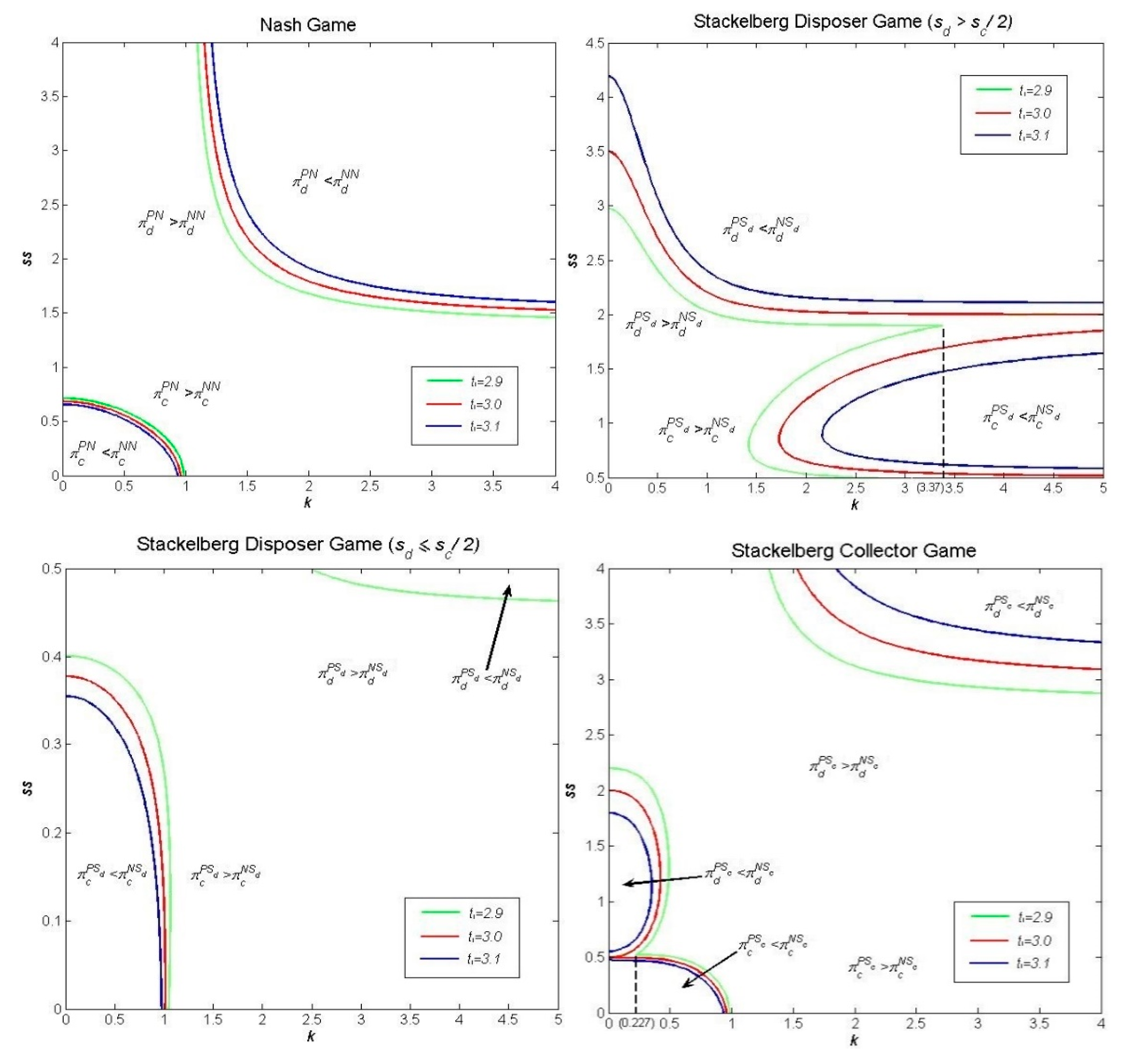
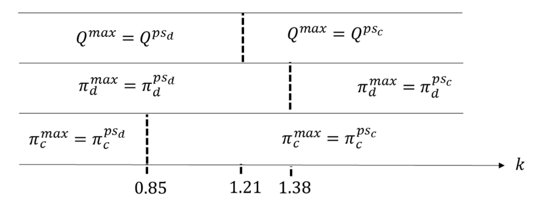
4.1. Conditions for Formation of Optimal Decision-Making of RSC in Two Models

In Joint Model, considering that the take-back price cannot be less than zero (the collector cannot charge fees on returning behavior), the thresholds of $s$ in different games are obtained (

Table 3. The condition for the formation of optimal decision-making of the RSC in two models.

Models	Nash	Stackelberg Disposer	Stackelberg Collector	Cooperation
Joint Model	$s>\frac{2\alpha }{\beta }$	$s>\frac{\alpha }{\beta }\frac{2-r}{r}$	$s>\frac{\alpha }{\beta }\frac{1+h}{1-h}$	$s>\frac{\alpha }{\beta }$
Single Model	$s_d>0$ $s_c>0$	$s_d>0$ $s_c>0$	$s_d>0$ $s_c>0$	$s>0$

). Note that the implementations of price incentives only simply require the sum of two member’s unit revenue ($s$) to meet certain conditions, because these models assume that the games are played in complete information scenarios, where both participants’ unit revenue are common knowledge. As a consequence, the unit revenue of one player ($s_d$ or $s_c$) can be less than 0 and $p_d$ plays the role in adjusting the profit margin ($m$ and $n$) between the members.

While in Single Model, since the RSC does not consider a take-back price incentive, the optimal solutions of $p_d$ in Nash, Stackelberg disposer, and Stackelberg collector are all equal to zero. Consequently, in these three games, the unit revenue of each player should be positive, or their total profits will be less than 0. In addition, the condition for cooperation game in Single Model is the lowest, where $s$ needs to be greater than zero.

Next, we further analyze the thresholds of $s$ to implement take-back price incentive in Joint Model. In the Nash game and the cooperation game, the threshold of $s$ is only related to $\alpha /\beta$, while in games of Stackelberg disposer and Stackelberg collector, besides the ratio, the thresholds are also affected by k, which is the relative strength of their advertising effectiveness. In the Stackelberg disposer game, the threshold of $s$ is increasing with k, which means it is more difficult to offer a price incentive to customers. In addition, this value is twice to three times that of the cooperation game. Meanwhile, it is opposite in the Stackelberg collector game, in which the threshold of $s$ is negatively correlated to changes in k. The better the disposer’s advertising effectiveness, the easier the collector provides the price incentives. Moreover, cooperation of the RSC leads to the lowest level of threshold s. Figure 3 depicts thresholds of $s$ respect to k in different games of Joint Model ($\alpha /\beta =1)$.

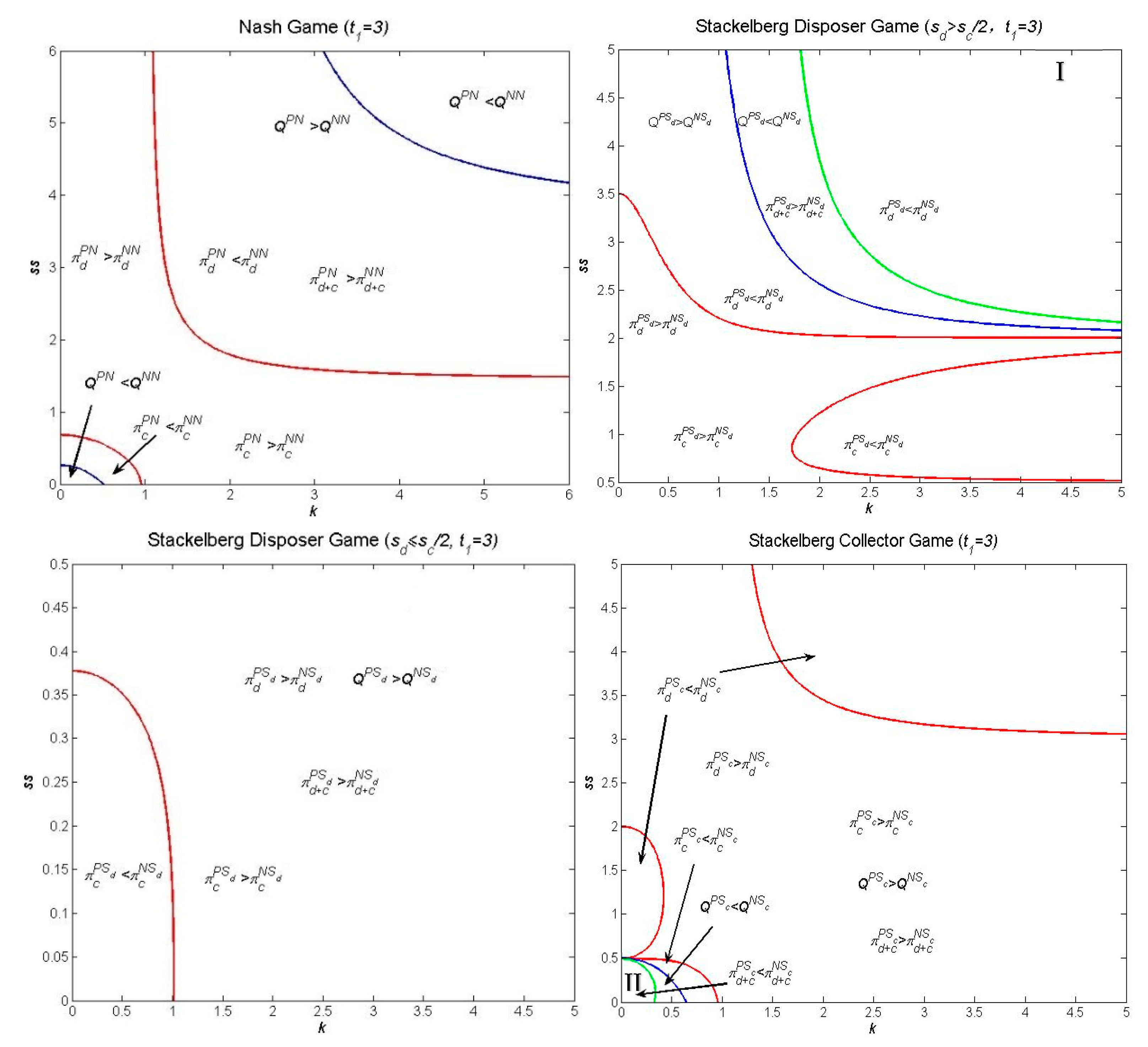
4.2. Comparison of the Two Models

In Section 4.1, we solved the questions if the games in the two models could be played. However, to a certain game, for instance, the Nash game, when both models can be played (i.e. conditions in Table 3 are satisfied under each game), does it always gain large quantity of collected UMs and more players’ profits to offer UMs holders price incentive (Joint Model)? This issue is settled by comparison of the two models in this section. (Optimal expressions in each game scenario of two models are shown in Appendix A).

Supposing $s_d,s_c>0$ and denoting $t_1=s\beta /\alpha$, $ss=s_d/s_c$ and $k=K_d/K_c$, the following propositions are provided. The details of proofs of Proposition 1–4 can be derived in Appendix B.

Proposition 1.

In the Nash game, in the range of $t_1>2$ , both players’ profits in Joint Model are always higher than those in Single Model when the following constraints are satisfied.

$$\{\begin{array}{c}\frac{{\left(1+t_1\right)}^4}{81t_1^2}{\left(1+ss\right)}^2\left(2+k^2\right)-\left(2ss+k^{2}s{s}^2\right)>0\\ \frac{{\left(1+t_1\right)}^4}{81t_1^2}{\left(1+ss\right)}^2\left(1+2k^2\right)-\left(1+2k^{2}ss\right)>0\end{array}$$

(30)

The first constraint is derived from ${\pi }_d^{PN}>{\pi }_d^{NN}$ and the second results from ${\pi }_c^{PN}>{\pi }_c^{NN}$.

Proposition 2.

In the Stackelberg disposer game, suppose $t_1>(2-r)/r$, then both players’ profits in Joint Model are always higher than those in Single Model when following constraints are satisfied.

When $s_d>s_c/2$,

$$\{\begin{array}{c}\frac{{\left(1+t_1\right)}^4{\left(1+ss\right)}^2{r}^2}{16t_1^2}\left[\frac{{\left(4-3r\right)}^2}{4}+4k^2{\left(1-r\right)}^2\right]-{\left(\frac{1}{2}+ss\right)}^2-k^{2}s{s}^2>0\\ \frac{{\left(1+t_1\right)}^4{\left(1+ss\right)}^2{r}^3}{16t_1^2}\left[\frac{\left(4-3r\right)}{4}+4k^2\left(1-r\right)\right]-s-2kss-\frac{1}{2}>0\end{array}$$

(31)

When $s_d\le s_c/2$,

$$\{\begin{array}{c}\frac{{\left(1+t_1\right)}^4{\left(1+ss\right)}^2{r}^2}{16t_1^2}\left[\frac{{\left(4-3r\right)}^2}{4}+4k^2{\left(1-r\right)}^2\right]-\left(2ss+k^{2}s{s}^2\right)>0\\ \frac{{\left(1+t_1\right)}^4{\left(1+ss\right)}^2{r}^3}{16t_1^2}\left[\frac{\left(4-3r\right)}{4}+4k^2\left(1-r\right)\right]-\left(1+2k^{2}ss\right)>0\end{array}$$

(32)

Similarly, the first inequalities in both cases are derived from ${\pi }_d^{P{S}_d}>{\pi }_d^{N{S}_d}$ and the second come from ${\pi }_c^{P{S}_d}>{\pi }_c^{N{S}_d}$. The two cases is caused by Single Model in which the disposer would like to share part of the collector’s advertising expenditure only when $s_d>s_c/2$. $t_1>(2-r)/r$ ensures that Joint Model can be played. In the range of $2<t_1<3$, assume that $k_0$ makes $t_1=(2-r)/r$. Since $(2-r)/r$ is increasing with respect to k, $t_1>(2-r)/r$ holds when $k<k_0$. When $t_1\ge 3$, k can be arbitrary.

Proposition 3.

In the Stackelberg collector game, suppose $t_1>(1+h)/(1-h)$, then both players’ profits in Joint Model are always higher than those in Single Model when following constraints are satisfied:

$$\{\begin{array}{c}\frac{{\left(1+t_1\right)}^4{\left(1+ss\right)}^2{\left(1-h\right)}^3}{16t_1^2}\left[4h+k^2\left(1-h\right)\right]-2ss-k^{2}s{s}^2>0\\ \frac{{\left(1+t_1\right)}^4{\left(1+ss\right)}^{2}h{\left(1-h\right)}^2}{4t_1^2}\left[h+k^2\left(1-h\right)\right]-1-2k^{2}ss>0\end{array}$$

(33)

The first inequality is introduced from ${\pi }_d^{P{S}_c}>{\pi }_d^{N{S}_c}$ and the second is derived from ${\pi }_c^{P{S}_c}>{\pi }_c^{N{S}_c}$. Similar to the Stackelberg disposer game, $t_1>(1+h)/(1-h)$ is to ensure that Joint Model can be played. In the range of $5/3<t_1<3$, it is assumed that $k_0$ makes $t_1=(1+h)/(1-h)$, since $(1+h)/(1-h)$ is decreasing with respect to k, $t_1>(1+h)/(1-h)$ holds when $k>k_0$. When $t_1\ge 3$, k can be arbitrary.

Since the implicit function forms of the conditional expression are inconvenient for analysis, some numerical examples are given. The expressions in Proposition 1–3 are with respect to three parameters, $t_1$, $ss$, and k. $t_1$ reflects the whole unit revenue of RSC, while $ss$ describes the allocation of this whole unit revenue in two players. k represents the relative effectiveness of disposer’s national advertising to collector’s local advertising. Set $t_1$ as a constant value and make the sensitivity analysis on $ss$ and k. Figure 4 depicts the comparisons of two players’ profits of two models in different games.

The lines denote relations of equality and divide the considered region into several areas. For example, the first figure describes the situations in the Nash game and there exist two lines. The top right one is ${\pi }_d^{PN}={\pi }_d^{NN}$ and it splits the whole region into two areas with ${\pi }_d^{PN}>{\pi }_d^{NN}$ on the left and ${\pi }_d^{PN}<{\pi }_d^{NN}$ on the right. As a consequence, the central area, where both two members’ profits in Joint Model are larger than those in Single Model, is the Pareto improvement area of Joint Model compared to Single Model. Interestingly, there is no area where both members’ profits in Single Model are larger than those in Joint Model simultaneously which means Single Model has no Pareto improving range to Joint Model in any game.

In each game, we choose three different values of $t_1$(2.9, 3 and 3.1). Regardless of the game, raising the overall unit revenue (the growth of $t_1$ indicates an increasing in $s$) can increase application range of Joint Model (more extensive $s$ and $k$), which suggests that the larger the $s$, the more the RSC of UMS should consider choosing Joint Model to offer UMs holders a take-back price incentive, which can increase both players’ profit.

Note that in the Stackelberg disposer game ($s_d>s_c/2$), when $t_1<3$, $k$ is not arbitrary for the constraint $t_1\ge (2-r)/r$. In this computation of $t_1=2.9$, k should be less than 3.37. Similarly, in the Stackelberg collector game of $t_1=2.9$, k should be more than 0.227.

Furthermore, in Pareto improvement area of Joint Model, not only both members’ profits are predominant, but also the quantity of collected UMs is more than that in Single Model (See Figure 5).

The green lines in the Stackelberg disposer game ($s_d>s_c/2$) and the Stackelberg collector game in Figure 5 are shaped by the equalities of total RSC profit in two models. There exists a region in each of the two games that the total RSC profit of Single Model is larger than that in Joint Model (Region I and II). However, in these regions, the total RSC profit increases, the leader’s profit increases, but the follower’s profit decreases. Then, the follower may refuse to join in the RSC of UMs in Single Model.

The Pareto dominant region combination of $ss$ and $k$ can be a reference for the government to make a subsidy policy for the collection of UMs. For instance, a RSC composed of a pharmaceutical manufacturer and a pharmacy and the manufacturer leads the game. The total unit revenue (s) only comes from the subsidies of the government. If the government considers the two parties’ advertising effectiveness is similar ($K_d=K_c$), then it is better for him to provide subsidies to not only the manufacturer but also the pharmacy (when $k=1$, the Pareto dominant region requires $ss$ be less than about 2.25). In turn, the government can choose the best RSC structure by the Pareto dominant region based on given $ss$ and $k$ practical situation.

Through the analysis of numerical examples above, it turns out that in decentralized games, it does not always gain more profit for each player and quantity of collected UMs to implement price incentive. However, comparing the results of the two models in the centralized game, we have the following observation.

Proposition 4.

When $s>\alpha /\beta$, $Q_{}^{PC}>Q_{}^{NC}$ and ${\pi }_{d+c}^{PC}>{\pi }_{d+c}^{NC}$.

Through the analysis of the numerical examples above, it turns out that in decentralized games, it does not always gain more profit for each player and quantity of collected UMs to implement a price incentive. However, comparing the results of the two models in the centralized game, we have the following observation.

Proposition 4 shows that in the cooperation game, when the condition to implement price incentive ($s>\alpha /\beta$) is achieved, the RSC should choose Joint Model and consider offering UMs take-back price incentive which may reach a higher quantity of collected UMs and total supply chain profit.

4.3. Comparisos within Joint Model

From the analysis of Section 4.1, it has determined that the whole unit revenue of the RSC should achieve a specific threshold to perform a take-back price incentive model (Joint Model). This section compares the optimal solutions including prices, advertising expenditures, quantity of collected UMs, and members’ profits in different game scenarios of Joint Model. Then, the feasibility of the cooperative games is explored in Section 4.3.4. The comparisons are on the base of an assumption that the thresholds in Section 4.1 of Joint Model have been achieved with all k, namely, $s>3\alpha /\beta$. The optimal solutions are summarized and presented in

Table A1. Optimal expressions in each game scenario in models with customers’ take-back price incentive (Joint Model).

Variables	Nash	Stackelberg Disposer	Stackelberg Collector	Cooperation
$p_d$	$\frac{2\beta s_d-\beta s_c-{\alpha }^{}}{3\beta }$	$\frac{r\beta s_d-\left(1-r\right)\beta s_c-\left(1-r\right)\alpha }{\beta }$	$\frac{\beta s_d\left(1+h\right)-\left(1-h\right)\beta s_c-\left(1-h\right)\alpha }{2\beta }$	N/A
$p_c$	$\frac{\beta s^{}-2{\alpha }^{}}{3\beta }$	$\frac{r\beta s-\left(2-r\right)\alpha }{2\beta }$	$\frac{\left(1-h\right)\beta s-\left(1+h\right)\alpha }{2\beta }$	$\frac{\beta s^{}-\alpha }{2\beta }$
$\sqrt{a}$	$\frac{K_c{\left(\beta s+\alpha \right)}^2}{18\beta }$	$\frac{K_c{\left(\beta s+\alpha \right)}^{2}r\left(4-3r\right)}{16\beta }$	$\frac{K_c{\left(\beta s+\alpha \right)}^{2}h\left(1-h\right)}{4\beta }$	$\frac{K_c{\left(\beta s+\alpha \right)}^2}{8\beta }$
$\sqrt{A}$	$\frac{K_d{\left(\beta s+\alpha \right)}^2}{18\beta }$	$\frac{K_d{\left(\beta s+\alpha \right)}^{2}r\left(1-r\right)}{4\beta }$	$\frac{K_d{\left(\beta s+\alpha \right)}^2{\left(1-h\right)}^2}{8\beta }$	$\frac{K_d{\left(\beta s+\alpha \right)}^2}{8\beta }$
$t$	$0$	$\frac{4-5r}{4-3r}$	$0$	N/A
$Q$	$\frac{{\left(\beta s+\alpha \right)}^3\left(K_c^2+K_d^2\right)}{54\beta }$	$\frac{{\left(\beta s+\alpha \right)}^3{r}^2}{16\beta }\left[K_c^2\frac{\left(4-3r\right)}{2}+K_d^{2}2\left(1-r\right)\right]$	$\frac{{\left(\beta s+\alpha \right)}^3{\left(1-h\right)}^2}{16\beta }\left[K_c^{2}2h+K_d^2\left(1-h\right)\right]$	$\frac{{\left(\beta s+\alpha \right)}^3\left(K_c^2+K_d^2\right)}{16\beta }$
${\pi }_d$	$\frac{{\left(\beta s+\alpha \right)}^4\left(2K_c^2+K_d^2\right)}{324{\beta }^2}$	$\frac{{\left(\beta s+\alpha \right)}^4{r}^2}{64{\beta }^2}\left[K_c^2{\left(4-3r\right)}^2/4+K_d^{2}4{\left(1-r\right)}^2\right]$	$\frac{{\left(\beta s+\alpha \right)}^4{\left(1-h\right)}^3}{64{\beta }^2}\left[K_c^{2}4h+K_d^2\left(1-h\right)\right]$	N/A
${\pi }_c$	$\frac{{\left(\beta s+\alpha \right)}^4\left(K_c^2+2K_d^2\right)}{324{\beta }^2}$	$\frac{{\left(\beta s+\alpha \right)}^4{r}^3}{64{\beta }^2}\left[K_c^2\frac{\left(4-3r\right)}{2}+K_d^{2}4\left(1-r\right)\right]$	$\frac{{\left(\beta s+\alpha \right)}^{4}h{\left(1-h\right)}^2}{16{\beta }^2}\left[K_c^{2}h+K_d^2\left(1-h\right)\right]$	N/A
${\pi }_{d+c}$	$\frac{{\left(\beta s+\alpha \right)}^4\left(K_c^2+K_d^2\right)}{108{\beta }^2}$	$\frac{{\left(\beta s+\alpha \right)}^4{r}^2}{64{\beta }^2}\left[K_c^2\frac{\left(4-3r\right)\left(4-r\right)}{4}+K_d^{2}4\left(1-r\right)\right]$	$\frac{{\left(\beta s+\alpha \right)}^4{\left(1-h\right)}^2}{64{\beta }^2}\left[K_c^{2}4h+K_d^2\left(1-h\right)\left(1+3h\right)\right]$	$\frac{{\left(\beta s+\alpha \right)}^4\left(K_c^2+K_d^2\right)}{64{\beta }^2}$
Collection efficiency	$\frac{8}{27}$	$\frac{r^2\left[\left(4-3r\right)/2+2k^2\left(1-r\right)\right]}{1+k^2}$	$\frac{{\left(1-h\right)}^2\left[2h+k^2\left(1-h\right)\right]}{1+k^2}$	N/A
Channel efficiency	$\frac{16}{27}$	$\frac{r^2\left[\left(4-3r\right)\left(4-r\right)/4+k^{2}4\left(1-r\right)\right]}{1+k^2}$	$\frac{{\left(1-h\right)}^2\left[4h+k^2\left(1-h\right)\left(1+3h\right)\right]}{1+k^2}$	N/A
${\pi }_d/{\pi }_c$	$1$	$\frac{{\left(4-3r\right)}^2/4+k^{2}4{\left(1-r\right)}^2}{r\left[\left(4-3r\right)/2+k^{2}4\left(1-r\right)\right]}$	$\frac{(1-h)\left[4h+k^2\left(1-h\right)\right]}{4h\left[h+k^2\left(1-h\right)\right]}$	N/A

Note: 1. Collection efficiency = $Q^{+}/Q^c$. 2. Channel efficiency = ${\pi }_{d+c}^{+}/{\pi }_{d+c}^C$. + stands for a game of Nash, Stackelberg disposer or Stackelberg collector.

in Appendix A. and the proofs of proposition 5–11 are shown in Appendix B.

4.3.1. Comparisons on Prices

Proposition 5.

The take-back prices in four game scenarios have the following ordinal relationship. (1) $p_c^{PC}>p_c^{PN}>p_c^{P{S}_d}\ge p_c^{P{S}_c}$, if $0<k\le k_1$ ; (2) $p_c^{PC}>p_c^{PN}\ge p_c^{P{S}_c}>p_c^{P{S}_d}$, if $k_1<k\le 1$ ; (3) $p_c^{PC}>p_c^{P{S}_c}>p_c^{PN}>p_c^{P{S}_d}$, if $k>1$. ( $k_1$ satisfies that $r+h=1$ ($k_1\approx 0.7164$)).

Proposition 5 reveals that the ordinal relationships of the take-back prices simply depend on k and are irrelevant to $s,s_d,s_c,\alpha \mathrm{and}\beta$. From the following Propositions 6 to 11, which are about $p_d,a,A,Q,{\pi }_c\mathrm{and}{\pi }_d$, their ordinal relationships merely rely on k and are independent of other parameters. It shows that the highest take-back price is always in the cooperative game whereas the lowest prices occur in the Stackelberg disposer game when k is lower ($k_1<0.7164$), and in the Stackelberg collector game when k is higher ($k_1>0.7164$). The take-back price offered to the UMs holders can be regarded as a kind of welfare and the increasing of the price would add the surplus of UMs holders.

Proposition 6.

The prices given to the collector by the disposer in four game scenarios have the following ordinal relationship. (1) $p_d^{P{S}_c}\ge p_d^{PN}>p_d^{P{S}_d}$, if $0<k\le 1$; (2) $p_d^{PN}\ge p_d^{P{S}_c}>p_d^{P{S}_d}$, if $1<k$.

From Proposition 6, regardless of k, the price in Stackelberg disposer game is the lowest indicating the leader position. When the effectiveness of the disposer’s national advertising is lower than that of the collector’s local advertising, the price is the highest in Stackelberg collector game, and followed by the Nash game.

4.3.2. Comparisons on Advertising Expenditures

Proposition 7.

The collector’s advertising expenditures in four game scenarios have the following ordinal relationship. (1) $a^{PC}>a^{P{S}_d}>a^{P{S}_c}\ge a^{PN}$, if $0<k\le 1$; (2) $a^{PC}>a^{P{S}_d}>a^{PN}>a^{P{S}_c}$, if $1<k$.

Proposition 7 concludes that in cooperative game, the collector’s local advertising expenditure is the highest and followed by Stackelberg disposer game. From Section 4.2, the disposer does not provide any collector’s advertising expenditure share in the Nash and the Stackelberg collector games. However, in the Stackelberg disposer game, he prefers sharing local advertising expenditure with the collector according to their relative advertising effectiveness. This expenditure sharing may result in the collector’s willingness to increase investment in advertising compared with the other two games.

Proposition 8.

The disposer’s advertising expenditures in four game scenarios have the following ordinal relationship. (1) $A^{PC}>A^{P{S}_d}>A^{PN}\ge A^{P{S}_c}$, if $0<k\le 1$; (2) $A^{PC}>A^{P{S}_d}>A^{P{S}_c}>A^{PN}$, if $1<k\le k_2$; (3) $A^{PC}>A^{P{S}_c}>A^{P{S}_d}>A^{PN}$, if $k_2<k$. ($k_2$ satisfies $2r(1-r)={(1-h)}^2$ ($k_2\approx 1.338$ )).

Similarly, based on Proposition 8, the disposer’s national advertising investment is the highest in the cooperative game and followed by the Stackelberg disposer game or the Stackelberg collector game. The disposer always invests more in the Stackelberg game as a leader than in the Nash game.

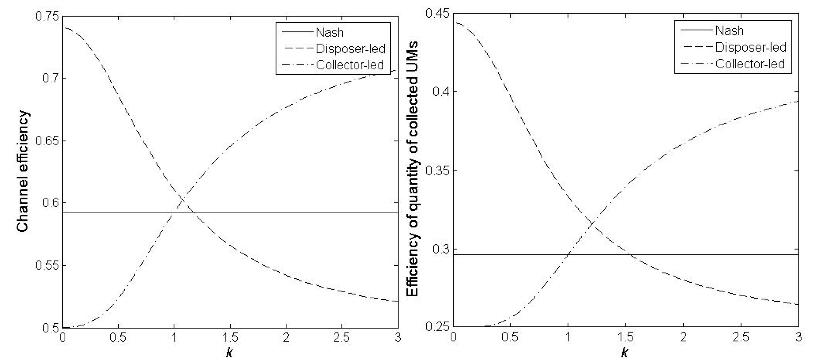
4.3.3. Comparisons on Quantity of Collected UMs and Profits

Proposition 9.

The quantity of collected UMs in four game scenarios have the following ordinal relationship. (1) $Q^{PC}>Q^{P{S}_d}>Q^{PN}\ge Q^{P{S}_c}$, if $0<k\le 1$; (2) $Q^{PC}>Q^{P{S}_d}\ge Q^{P{S}_c}>Q^{PN}$, if $1<k\le k_3$; (3) $Q^{PC}>Q^{P{S}_c}>Q^{P{S}_d}\ge Q^{PN}$, if $k_3<k\le k_4$; (4) $Q^{PC}>Q^{P{S}_c}>Q^{PN}>Q^{P{S}_d}$, if $k_4\text{<}k$. ($k_3$ satisfies $r^2\left[\left(4-3r\right)/2+k^{2}2\left(1-r\right)\right]={\left(1-h\right)}^2\left[2h+k^2\left(1-h\right)\right]$ ($k_3\approx 1.2060$); $k_4$ satisfies $8\left(1+k^2\right)=27r^2\left[\left(4-3r\right)/2+k^{2}2\left(1-r\right)\right]$ ($k_4\approx 1.5385$)).

The largest amount of collected UMs is also from the cooperative game, followed by the Stackelberg disposer or the Stackelberg collector, instead of Nash game. It is evident from Proposition 9 that when $k<1.21$, the quantity of collected UMs in the Stackelberg disposer game is more than other two games and when $k>1.21$, it is in the Stackelberg collector game that the quantity is the most.

Proposition 10.

The disposers’ profits in four game scenarios have the following ordinal relationship. (1) ${\pi }_d^{P{S}_d}\text{>}{\pi }_d^{PN}\ge {\pi }_d^{P{S}_c}$, if $0<k\le 1$; (2) ${\pi }_d^{P{S}_d}\ge {\pi }_d^{P{S}_c}>{\pi }_d^{PN}$, if $1<k\le k_5;$ (3) ${\pi }_d^{P{S}_c}>{\pi }_d^{P{S}_d}\text{>}{\pi }_d^{PN}$, if $k_5\text{<}k$. ($k_5$ satisfies $r^3\left[\left(4-3r\right)/2+k^{2}4\left(1-r\right)\right]=4h{\left(1-h\right)}^2\left[h+k^2\left(1-h\right)\right]$ ($k_5\approx 1.3835$)).

It is obvious from Proposition 10 that the disposer prefers the leader-follower structure (the Stackelberg disposer game or the Stackelberg collector game) rather than the simultaneous move structure (the Nash game). If the disposer’s advertising effectiveness is relatively weak ($k<1.3835$), he tends to lead the game to obtain more channel profit, while if his advertising effectiveness is comparatively high, he would like to be a follower, which makes him gain more profit.

Proposition 11.

The collectors’ profits in four game scenarios have the following ordinal relationship. (1) ${\pi }_c^{P{S}_d}\ge {\pi }_d^{P{S}_c}\text{>}{\pi }_d^{PN}$, if $0<k\le k_6$; (2) ${\pi }_d^{P{S}_c}\ge {\pi }_d^{P{S}_d}>{\pi }_d^{PN}$, if ${\mathrm{k}}_6<k\le k_7$; (3) ${\pi }_d^{P{S}_c}>{\pi }_d^{PN}\text{>}{\pi }_d^{P{S}_d}$, if $k_7\text{<}k$. $(k_6\mathrm{satisfies}{r}^3\left[\left(4-3r\right)/2+k^{2}4\left(1-r\right)\right]=4h{\left(1-h\right)}^2\left[h+k^2\left(1-h\right)\right]$ $(k_6\approx 0.8457);$ $k_7\mathrm{satisfies}16\left(1+2k^2\right)=81r^3\left[\left(4-3r\right)/2+4k^2\left(1-r\right)\right](k_7\approx 0.8552))$.

Proposition 11 reveals that the collector has an aptitude for being a leader when $k>0.85$ and being a follower when $k<0.85$, which can bring her more profit. Thus, combining Proposition 10 and Proposition 11, it demonstrates that there exist accordance and conflict in the leader-follower structure (Figure 6). More specifically, when $k<0.85$, the disposer prefers being a leader in the RSC and precisely the collector is willing to be a follower. In this structure, both players can gain their maximum profit in non-cooperative games. Similarly, if $k>1.38$, a game structure with the collector as the leader and the disposer as the follower is both members’ preference. Therefore, these two ranges are their accordance regions. However, if $0.85<k<1.38$, the two players’ optimal profits are all in their own leading game, which resulted in a conflict with each other rather than being a Stackelberg follower. It is worth mentioning that in this conflict region, if $k<1.12$, the quantity of collected UMs is largest in the Stackelberg disposer game, which is better for the collecting activity.

Besides, the collection efficiency and channel efficiency are analyzed, and calculated as the ratio of non-cooperative games to the cooperative game and the sum of two players’ profits in any of the non-cooperative games to the total profit of RSC in the cooperative game solution (see Figure 7). From Figure 7, the following proposition is presented.

Proposition 12.

The coordination of the Stackelberg disposer game and the Stackelberg collector game decreases and increases with k, respectively, while it is independent with k in the Nash game.

The cooperative game is a more coordinated model than the non-cooperative games. When the collector’s advertising is more efficient, a more coordinated model will return a higher profit to the RSC in the Stackelberg disposer game. By contrast, when the disposer’s advertising is more efficient, the Stackelberg collector game is more coordinated.

In summary, the analytical results favor that cooperative game which is the best at offering the highest take-back price and invest the most in both national and local advertising, leading to the most preferable collected quantity and total profit. Furthermore, in non-cooperative games, it is better to implement the leader-follower structure rather than simultaneous movement structure. In details, when the disposer’s national advertising effect is relatively lower than the collector’s, the Stackelberg disposer game would be more satisfactory. However, if the disposer’s advertising is efficient, a Stackelberg collector game is favorable.

4.3.4. Feasibility of the Cooperation

With the analytical solutions of the cooperative game in Section 3.1.4, it is observed that the disposer and the collector would only agree to make joint decisions if their individual profits are higher in the cooperative game than those in the non-cooperative structures. In this section, the comparative results in Section 4.3 are applied to verify the feasibility of the problem. To achieve this, it is necessary to prove the existence of $\left(p_c^{PC},p_d^{PC},a^{PC},A^{PC},t^{PC}\right)$. Based on Equation (29), it derives

$${\pi }_{d+c}^{PC}\ge {\pi }_d^{\max }+{\pi }_c^{\max }$$

(34)

Based on Proposition 10 and Proposition 11, the maximum profits of the disposer and collector are obtained in three regions.

Table 4. The maximum profits of the disposer and the collector.

$\mathit{k}$	${\mathit{\pi }}_{\mathit{d}}^{\mathit{max}}$	${\mathit{\pi }}_{\mathit{c}}^{\mathit{max}}$
$k\le 0.85$	${\pi }_d^{P{S}_d}$	${\pi }_c^{P{S}_d}$
$0.85<k<1.38$	${\pi }_d^{P{S}_d}$	${\pi }_c^{P{S}_c}$
$1.38\le k$	${\pi }_d^{P{S}_c}$	${\pi }_c^{P{S}_c}$

determines the maximum profits of each player in each region.

It is evident that when $k\le 0.85$ and $k\ge 1.38$, the inequality Equation (34) is obtained, because ${\pi }_d^{\max }+{\pi }_c^{\max }$ equals to ${\pi }_{d+c}^{P{S}_d}$ and ${\pi }_{d+c}^{P{S}_c}$ respectively and they are all less than ${\pi }_{d+c}^{PC}$. Similarly, the ratio $({\pi }_d^{P{S}_d}+{\pi }_c^{P{S}_c})/{\pi }_{d+c}^{PC}$ can be calculated as being less than 1 in the range of $0.85<k<1.38$. Consequently, it shows that the cooperative game is feasible, which leads to the disposer and the collector’s willingness to cooperate. Therefore, next section will make a trial to settle the problem that how to share the extra profit from cooperation. The profit-sharing issue is discussed in Section 4.3.5.

4.3.5. Bargaining Model

In this section, a feasible region is proposed for the two internal variables $p_d$ and t. Then, the Nash bargaining model will be conducted to resolve the profit-sharing problem in this region. The feasible region for this problem can be clarified based on the method used by Xie and Wei [28]. The extra profit of the disposer and the collector are as follows:

$$\begin{array}{cc}\hfill \Delta {\pi }_d& ={\pi }_d^{PC}-{\pi }_d^{\max }\hfill \\ & =\left(s_d-p_d\right)\left(\alpha +\beta p_c^{PC}\right)\left(K_c\sqrt{a^{PC}}+K_d\sqrt{A^{PC}}\right)-A^{PC}-t{a}^{PC}-{\pi }_d^{\max }\hfill \\ & =-p_{d}B-t{a}^{PC}+C>0\hfill \end{array}$$

(35)

$$\begin{array}{cc}\hfill \Delta {\pi }_c& ={\pi }_c^{PC}-{\pi }_c^{\max }\hfill \\ & =\left(p_d+s_c-p_c^{PC}\right)\left(\alpha +\beta p_c^{PC}\right)\left(K_c\sqrt{a^{PC}}+K_d\sqrt{A^{PC}}\right)-\left(1-t\right)a^{PC}-{\pi }_c^{\max }\hfill \\ & =p_{d}B+t{a}^{PC}-D>0\hfill \end{array}$$

(36)

where B, C, and D are $B=\left(\alpha +\beta p_c^{PC}\right)\left(K_c\sqrt{a^{PC}}+K_d\sqrt{A^{PC}}\right)>0$, $C=s_{d}B-A^{PC}-{\pi }_d^{\max }>0$ and $D=-\left(s_c-p_c\right)B+a^{PC}+{\pi }_c^{\max }>0$.

Thus, it shows that inequalities (35) and (36) specify an area between two parallel lines. Every combination $\left(p_d,t\right)$ in this region presents a feasible solution to the bargaining problem. According to Nash [39], the bargaining outcome $(p_d^{*},t^{*})$ can be obtained by maximizing the product of player’s utilities over the feasible solution. ${\lambda }_d$ and ${\lambda }_c$ can be regarded as the bargaining power of the disposer and collector, respectively. Thus, the utility functions for the disposer and the collector are $u_d\left(p_d,t\right)=\Delta {\pi }_d{\left(p_d,t\right)}^{{\lambda }_d},u_c\left(p_d,t\right)=\Delta {\pi }_c{\left(p_d,t\right)}^{{\lambda }_c}$, respectively.

Then Nash’s solution can be derived from the following optimization,

$$\max u_d\left(p_d,t\right)\cdot u_c\left(p_d,t\right)=\Delta {\pi }_d{\left(p_d,t\right)}^{{\lambda }_d}\cdot \Delta {\pi }_c{\left(p_d,t\right)}^{{\lambda }_c}$$

(37)

The solution of Equation (37) is achieved:

$$\begin{array}{l}\Delta {\pi }_d\left(p_{{}_d}^{*},t^{*}\right)=\frac{{\lambda }_d}{{\lambda }_d+{\lambda }_c}\Delta {\pi }_{d+c}=\frac{{\lambda }_d}{{\lambda }_d+{\lambda }_c}\left(C-D\right),\\ \Delta {\pi }_c\left(p_{{}_d}^{*},t^{*}\right)=\frac{{\lambda }_c}{{\lambda }_d+{\lambda }_c}\Delta {\pi }_{d+c}=\frac{{\lambda }_c}{{\lambda }_d+{\lambda }_c}\left(C-D\right).\end{array}$$

(38)

Therefore, if ${\lambda }_d>{\lambda }_c$, the disposer shares more extra profit than the collector’s and the same $\lambda$ makes the two players equally divide profits. From Equation (38), it is easy to obtain

$$p_{{}_d}^{*}B+t^{*}{a}^{PC}=\frac{D{\lambda }_d+C{\lambda }_c}{{\lambda }_d+{\lambda }_c}$$

(39)

Equation (39) describes the relationship between the optimal solutions of $p_d$ and $t$ in the cooperative game, which is a line parallel to ${\pi }_d^{PC}={\pi }_d^{max}$.

4.4. Comparisons within Single Model

From

Table A2. Optimal expressions in each game scenario in models without customers’ take-back price incentive (Single Model).

Variables	Nash	Stackelberg Disposer	Stackelberg Collector	Cooperation
$p_d$	$0$	$0$	$0$	N/A
$p_c$	$0$	$0$	$0$	$0$
$\sqrt{a}$	$\frac{\alpha K_c{s}_c}{2}$	$\frac{\alpha K_c\left(2s_d+s_c\right)}{4}$	$\frac{\alpha K_c{s}_c}{2}$	$\frac{\alpha K_{c}s}{2}$
$\sqrt{A}$	$\frac{\alpha K_d{s}_d}{2}$	$\frac{\alpha K_d{s}_d}{2}$	$\frac{\alpha K_d{s}_d}{2}$	$\frac{\alpha K_{d}s}{2}$
$t$	$0$	$\frac{2s_d-s_c}{2s_d+s_c}$	$0$	N/A
$Q$	$\frac{{\alpha }^2}{2}\left(K_c^2{s}_c+K_d^2{s}_d\right)$	$\frac{{\alpha }^2}{2}\left[K_c^2\left(s_d+\frac{s_c}{2}\right)+K_d^2{s}_d\right]$	$\frac{{\alpha }^2}{2}\left(K_c^2{s}_c+K_d^2{s}_d\right)$	$\frac{{\alpha }^{2}s}{2}\left(K_c^2+K_d^2\right)$
${\pi }_d$	$\frac{{\alpha }^2}{4}\left(K_c^{2}2s_c{s}_d+K_d^2{s}_d^2\right)$	$\frac{{\alpha }^2}{4}\left[K_c^2{\left(s_d+\frac{s_c}{2}\right)}^2+K_d^2{s}_d^2\right]$	$\frac{{\alpha }^2}{4}\left(K_c^{2}2s_c{s}_d+K_d^2{s}_d^2\right)$	N/A
${\pi }_c$	$\frac{{\alpha }^2}{4}\left(K_c^2{s}_c^2+K_d^{2}2s_c{s}_d\right)$	$\frac{{\alpha }^2{s}_c}{4}\left[K_c^2\left(s_d+\frac{s_c}{2}\right)+2K_d^2{s}_d\right]$	$\frac{{\alpha }^2}{4}\left(K_c^2{s}_c^2+K_d^{2}2s_c{s}_d\right)$	N/A
${\pi }_{d+c}$	$\frac{{\alpha }^2}{4}\left[K_d^2{s}_d^2+K_c^2{s}_c^2+2s_c{s}_d\left(K_c^2+K_d^2\right)\right]$	$\frac{{\alpha }^2}{4}\left[\frac{K_c^2\left(2s_d+s_c\right)\left(2s_d+3s_c\right)}{4}+K_d^2{s}_d\left(2s_c+s_d\right)\right]$	$\frac{{\alpha }^2}{4}\left[K_d^2{s}_d^2+K_c^2{s}_c^2+2s_c{s}_d\left(K_c^2+K_d^2\right)\right]$	$\frac{{\alpha }^2{s}^2}{4}\left(K_c^2+K_d^2\right)$
Collection efficiency	$\frac{\left(1+k^{2}ss\right)}{\left(1+ss\right)\left(1+k^2\right)}$	$\frac{ss+1/2+k^{2}ss}{\left(1+ss\right)\left(1+k^2\right)}$	$\frac{\left(1+k^{2}ss\right)}{\left(1+ss\right)\left(1+k^2\right)}$	N/A
Channel efficiency	$\frac{k^{2}s{s}^2+1+2ss\left(1+k^2\right)}{{\left(1+ss\right)}^2\left(1+k^2\right)}$	$\frac{\left[\left(2ss+1\right)\left(2ss+3\right)+k^2\left(8ss+s{s}^2\right)\right]}{4{\left(1+ss\right)}^2\left(1+k^2\right)}$	$\frac{k^{2}s{s}^2+1+2ss\left(1+k^2\right)}{{\left(1+ss\right)}^2\left(1+k^2\right)}$	N/A
${\pi }_d/{\pi }_c$	$\frac{2ss+k^{2}s{s}^2}{1+2k^{2}ss}$	$\frac{{\left(ss+1/2\right)}^2+k^{2}s{s}^2}{2k^{2}ss+ss+1/2}$	$\frac{2ss+k^{2}s{s}^2}{1+2k^{2}ss}$	N/A

Note: The optimal solutions of Stackelberg disposer game are in the situation $s_d>s_c/2$. When $s_d\le s_c/2$, the results are the same as those in Nash equilibrium.

in Appendix A, it turns out that the optimal solutions are identical in the Nash game, the Stackelberg collector game, and the Stackelberg disposer game without cooperative advertising ($s_d/s_c\le 1/2$). Consequently, these optimal solutions are labeled as a superscript S+ and make comparisons on these same solutions with the Stackelberg disposer game with $s_d/s_c>1/2$.

Proposition 13.

In the model without take-back price incentive, the following ordinal relationships are always satisfied. (1) $a^{NC}>a^{N{S}_d}>a^{N{S}_{+}}$; (2) $A^{NC}>A^{N{S}_d}=A^{N{S}_{+}}$; (3) $Q^{NC}>Q^{N{S}_d}>Q^{N{S}_{+}}$; (4) ${\pi }_{\mathrm{c}}^{N{S}_d}>{\pi }_c^{N{S}_{+}}$; (5) ${\pi }_d^{N{S}_d}>{\pi }_d^{N{S}_{+}}$; (6) ${\pi }_{d+c}^{NC}>{\pi }_{d+c}^{N{S}_d}>{\pi }_{d+c}^{N{S}_{+}}$.

From Proposition 13, it reveals that only when the unit revenue of the disposer is larger than half of the collector’s, the disposer prefers sharing the responsibility of the collector’s advertising expenditure, which leads to a better collective effect including more quantity of collected UMs and more profit for both members. Figure 8 presents the collection efficiency and channel efficiency of the Stackelberg disposer with cooperative advertising $(s_d/s_c>1/2)$. It shows that both efficiencies are high under the circumstance where $ss$ is large and $k$ is small. Especially, the channel efficiency is extremely close to 1, which means the coordination of RSC.

In summary, when the RSC does not consider offering a take-back price incentive, it is better for the disposer to undertake a channel leader position and the collector acts as the follower. The disposer should choose a collector with better advertising effectiveness and share a proportion of the collector’s advertising expenditure. Besides, if the government would like to make a subsidy or penalty policy (the penalty can be treated as an opportunity cost to increase the unit revenue in turn) to the UMs RSC, it is favorable for him to aim at the disposer, for instance, the pharmaceutical manufacture, since it can increase the disposer’s unit revenue compared with the collector’s (an increase in $ss$).

5. Conclusions

For collecting more UMs from households, this study develops and tests two models in a RSC composed of a single disposer and a collector. In Joint Model, the quantity of collected UMs is affected by take-back price and advertising, while in Single Model, the quantity of collected UMs is influenced only by advertising. In each model, four games are played: non-cooperative, disposer as the Stackelberg leader, disposer as the Stackelberg leader, and cooperative. The conditions for the formation of optimal decision-making of the RSC in two models are explored.

In Single Model, both players’ unit revenue should be more than 0. Whereas the total unit revenue of the two players should be more than a specific threshold in Joint Model, and the price paid by the disposer to the collector adjusts their corresponding margin profit. In real life, most countries are currently adopting Single Model and do not offer take-back price. Therefore, it is hard for the disposers to get any revenue. If so, the disposers are not willing to pay any to the collectors to adjust collectors’ profit margin. How both players can receive benefits becomes a practical issue. Among all UMs, some UMs are unused but near expired. The RSC can offer a channel for disposers to pay extra money for replacing these kinds of UMs. After verifying the packages of these UMs, the collectors can sell these UMs in a good discount rate to the consumers who will use them immediately. This arrangement can satisfy the win-win requirement in Single Model. Of course, this suggestion is based on an assumption that regulation allows reselling reusable unexpired medications.

Comparing the equilibrium results in the four games of the two models, we conclude that, for a certain game, for instance the Nash game, when both models can be played, there always exists a Pareto dominance range with respect to the total unit revenue ($t_1$) and its allocation (ss) between two members and their relative effectiveness of advertising expenses (k) for Joint Model compared with Single Model, where more players’ profits and larger quantity of collected UMs can be obtained. Under these conditions, RSC prefers choosing Joint Model in which a take-back price should be considered offered to UMs holders. Therefore, offering take-back price can reduce the cost of advertising because less advertising is needed due to its effectiveness. If so, the RSC or the government can relocate its budget from doing advertising to giving a take-back price. So the RSC or the government does not really pay a big money for executing “take-back price” policy. On the other hand, the take-back price may not be instant “cash”. It can be in a form of a cash coupon for environmentally friendly grocery products. Therefore, it can promote a sustainable concept to the UMs holders. This arrangement can also be interpreted by the public as a way for the RSC or the government to support sustainable development by supporting the producers of environmentally friendly grocery products. Furthermore, the RSC or the government can set a one-to-one sustainability fund to subsidize poor people to purchase medications. When a UMs holder returns the UMs, the government will donate the same amount of money to the fund as the amount of “take-back price” to the UMs holder. This arrangement provides a good excuse for the UMs holders to return the UMs (not for money) and creates a good citizen image for these UMs holders.

However, there exists no area where both members’ profits in Single Model are larger than those in Joint Model simultaneously, which means Single Model has no Pareto improving range to Joint Model in any games. The cooperative game has the lowest implement threshold compared with other three games in Joint Model. Furthermore, when the condition to implement price incentive is achieved, regardless of $t_1$, ss, and k, the RSC should choose Joint Model to reach the higher quantity of collected UMs and total supply chain profit. As discussed above, in the real life, it is hard to design a practical strategy that can facilitate both parties to obtain a desirable amount of benefits in Single Model. However, for Joint Model, not limited to above recommendations, there are a lot of areas for the RSC and the government to implement price incentive strategy. However, in considering the effectiveness of Joint Model (in term of the quantity of collected UMs and total supply chain profit), the real cooperation of the RSC for UMs becomes a matter of cardinal significance.

Furthermore, the total unit revenue is vital to the RSC. The larger the total unit revenue, the more likely the two members are to implement a take-back price incentive where more quantity of collected UMs is achieved. In this research, it is assumed that it is positive which may form the driving force of the growth of sales in FSC and social responsibility [36]. Through the health promotion and education for disease prevention, more people will care about their health and know how to consume medications for improving their quality of life. Then, the sales of medications will grow. Social responsibility is a fundamental aspect of citizenship, so citizens are educated to participate in creating a safer, more humane, sustainable world. The education for social responsibility can take place in different structures and processes in communities. Another positive driving force is related law and regulation, such as the permission to resell reusable unexpired medications [37], so the government is taking a major role in implementing the “take-back price” in real life through revising the law and regulation.

In most cases, it is undeniable that this revenue is difficult to measure in reality and the immediate and obvious financial benefit is lacking compared with WEEE RSC. This situation calls for regulations and subsidies from the government who could levy a disposing tax on the pharmaceutical industry or medication users, and then assist the RSC for UMs. Kotchen et al. [40] made a survey to study the residents’ willingness to pay for a disposal program, and the results show that the conservative estimate of mean willingness to pay is $1.53 per prescription and this assumption implies $320 million for the United States as a whole, which easily outweighs the costs of establishing disposal programs.

This research has multiple limitations. When considering the pricing model, it chooses a simplest linear model. It may not be highly appropriate for the practice and needs further discussion. Besides, the total available quantity of collected UMs is not unlimited in reality, whereas the quantitative restriction is not taken into consideration and simply treated as unrestricted. However, it is usually insufficient to consider the fund for the collection of UMs and this assumption is of rationality. Furthermore, for the convenience of analysis, it is supposed that the collected UMs is homogeneous or can be explained as a mean value. Nevertheless, it does not conform to the reality and needs further research.

References

1. Belloni, A.; Morgan, D.; Paris, V. Pharmaceutical Expenditure and Policies: Past Trends and Future Challenges; OECD Publishing: Paris, France, 2016; ISSN 1815-2015 (online). Available online: http://0-www-oecd--ilibrary-org.brum.beds.ac.uk/social-issues-migration-health/pharmaceutical-expenditure-and-policies_5jm0q1f4cdq7-en (accessed on 31 August 2017).
2. Vellinga, A.; Cormican, S.; Driscoll, J.; Furey, M.; O’Sullivan, M.; Cormican, M. Public practice regarding disposal of unused medicines in ireland. Sci. Total Environ. 2014, 478, 98–102. [Google Scholar] [CrossRef] [PubMed]
3. Law, A.V.; Sakharkar, P.; Zargarzadeh, A.; Tai, B.W.; Hess, K.; Hata, M.; Mireles, R.; Ha, C.; Park, T.J. Taking stock of medication wastage: Unused medications in us households. Res. Soc. Adm. Pharm. 2015, 11, 571–578. [Google Scholar] [CrossRef] [PubMed]
4. World Health Organization (WHO). Guidelines for Safe Disposal of Unwanted Pharmaceuticals in and after Emergencies. Available online: http://apps.who.int/medicinedocs/en/d/Jwhozip51e/ (accessed on 31 August 2017).
5. Bound, J.P.; Nikolaos, V. Household disposal of pharmaceuticals as a pathway for aquatic contamination in the united kingdom. Environ. Health Perspect. 2005, 113, 1705–1711. [Google Scholar] [CrossRef] [PubMed]
6. Kümmerer, K. The presence of pharmaceuticals in the environment due to human use—Present knowledge and future challenges. J. Environ. Manage. 2009, 90, 2354–2366. [Google Scholar] [CrossRef] [PubMed]
7. Massoud, M.A.; Chami, G.; Al-Hindi, M.; Alameddine, I. Assessment of household disposal of pharmaceuticals in lebanon: Management options to protect water quality and public health. Environ. Manag. 2016, 57, 1125–1137. [Google Scholar] [CrossRef] [PubMed]
8. Musson, S.E.; Townsend, T.G. Pharmaceutical compound content of municipal solid waste. J. Hazard. Mater. 2009, 162, 730–735. [Google Scholar] [CrossRef] [PubMed]
9. Bu, Q.W.; Wang, B.; Huang, J.; Deng, S.B.; Yu, G. Pharmaceuticals and personal care products in the aquatic environment in china: A review. J. Hazard. Mater. 2013, 262, 189–211. [Google Scholar] [CrossRef] [PubMed]
10. Verlicchi, P.; Zambello, E. Pharmaceuticals and personal care products in untreated and treated sewage sludge: Occurrence and environmental risk in the case of application on soil—A critical review. Sci. Total Environ. 2015, 538, 750–767. [Google Scholar] [CrossRef] [PubMed]
11. Subedi, B.; Codru, N.; Dziewulski, D.M.; Wilson, L.R.; Xue, J.; Yun, S.; Braun-Howland, E.; Minihane, C.; Kannan, K. A pilot study on the assessment of trace organic contaminants including pharmaceuticals and personal care products from on-site wastewater treatment systems along skaneateles lake in new york state, USA. Water Res. 2015, 72, 28–39. [Google Scholar] [CrossRef] [PubMed]
12. European Union (EU). Directive 2001/83/EC of the European Parliament and of the Council of 6 November 2001 on the community code relating to medicinal products for human use. Off. J. L-311 2001, 67–128, article 127b. Available online: http://eur-lex.europa.eu/LexUriServ/LexUriServ.do?uri=CELEX:32001L0083:EN:HTML (accessed on 17 October 2017).
13. Directive 2004/27/EC of the European Parliament and of the Council of 31 March 2004 amending 2001/83/EC on the community code relating to medicinal products for human use. Off. J. Eur. Union 2004, 136, 34–57, article 127b. Available online: http://eur-lex.europa.eu/legal-content/EN/TXT/HTML/?uri=CELEX:32004L0027&qid=1508240342747&from=EN (accessed on 17 October 2017).
14. Glassmeyer, S.T.; Hinchey, E.K.; Boehme, S.E.; Daughton, C.G.; Ruhoy, I.S.; Conerly, O.; Daniels, R.L.; Lauer, L.; McCarthy, M.; Nettesheim, T.G.; et al. Disposal practices for unwanted residential medications in the united states. Environ. Int. 2009, 35, 566–572. [Google Scholar] [CrossRef] [PubMed]
15. Kozak, M.A.; Melton, J.R.; Gernant, S.A.; Snyder, M.E. A needs assessment of unused and expired medication disposal practices: A study from the medication safety research network of indiana. Res. Soc. Adm. Pharm. 2016, 12, 336–340. [Google Scholar] [CrossRef] [PubMed]
16. Abahussain, E.; Waheedi, M.; Koshy, S. Practice, awareness and opinion of pharmacists toward disposal of unwanted medications in kuwait. Saudi Pharm. J. 2012, 20, 195–201. [Google Scholar] [CrossRef] [PubMed]
17. Al-Shareef, F.; El-Asrar, S.A.; Al-Bakr, L.; Al-Amro, M.; Alqahtani, F.; Aleanizy, F.; Al-Rashood, S. Investigating the disposal of expired and unused medication in riyadh, saudi arabia: A cross-sectional study. Int. J. Clin. Pharm. 2016, 38, 822–828. [Google Scholar] [CrossRef] [PubMed]
18. Kusturica, M.P.; Sabo, A.; Tomic, Z.; Horvat, O.; Solak, Z. Storage and disposal of unused medications: Knowledge, behavior, and attitudes among serbian people. Int. J. Clin. Pharm. 2012, 34, 604–610. [Google Scholar] [CrossRef] [PubMed]
19. Jonjić, D.; Vitale, K. Issues around household pharmaceutical waste disposal through community pharmacies in croatia. Int. J. Clin. Pharm. 2014, 36, 556–563. [Google Scholar] [CrossRef] [PubMed]
20. Yoon, S.W.; Jeong, S.J. Implementing coordinative contracts between manufacturer and retailer in a reverse supply chain. Sustainability 2016, 8, 913. [Google Scholar] [CrossRef]
21. Xie, Y.; Breen, L. Who cares wins? A comparative analysis of household waste medicines and batteries reverse logistics systems. Supply Chain Manag. 2014, 19, 455–474. [Google Scholar] [CrossRef]
22. Aust, G.; Buscher, U. Cooperative advertising models in supply chain management: A review. Eur. J. Oper. Res. 2014, 234, 1–14. [Google Scholar] [CrossRef]
23. Jørgensen, S.; Zaccour, G. A survey of game-theoretic models of cooperative advertising. Eur. J. Oper. Res. 2014, 237, 1–14. [Google Scholar] [CrossRef]
24. Yue, J.F.; Austin, J.; Wang, M.C.; Huang, Z.M. Coordination of cooperative advertising in a two-level supply chain when manufacturer offers discount. Eur. J. Oper. Res. 2006, 168, 65–85. [Google Scholar] [CrossRef]
25. Szmerekovsky, J.G.; Zhang, J. Pricing and two-tier advertising with one manufacturer and one retailer. Eur. J. Oper. Res. 2009, 192, 904–917. [Google Scholar] [CrossRef]
26. Xie, J.X.; Neyret, A. Co-op advertising and pricing models in manufacturer-retailer supply chains. Comput. Ind. Eng. 2009, 56, 1375–1385. [Google Scholar] [CrossRef]
27. Chaab, J.; Rasti-Barzoki, M. Cooperative advertising and pricing in a manufacturer-retailer supply chain with a general demand function; a game-theoretic approach. Comput. Ind. Eng. 2016, 99, 112–123. [Google Scholar] [CrossRef]
28. Xie, J.X.; Wei, J.C. Coordinating advertising and pricing in a manufacturer-retailer channel. Eur. J. Oper. Res. 2009, 197, 785–791. [Google Scholar] [CrossRef]
29. SeyedEsfahani, M.M.; Biazaran, M.; Gharakhani, M. A game theoretic approach to coordinate pricing and vertical co-op advertising in manufacturer-retailer supply chains. Eur. J. Oper. Res. 2011, 211, 263–273. [Google Scholar] [CrossRef]
30. Kunter, M. Coordination via cost and revenue sharing in manufacturer-retailer channels. Eur. J. Oper. Res. 2012, 216, 477–486. [Google Scholar] [CrossRef]
31. Aust, G.; Buscher, U. Vertical cooperative advertising and pricing decisions in a manufacturer-retailer supply chain: A game-theoretic approach. Eur. J. Oper. Res. 2012, 223, 473–482. [Google Scholar] [CrossRef]
32. Zhao, L.; Zhang, J.H.; Xie, J.X. Impact of demand price elasticity on advantages of cooperative advertising in a two-tier supply chain. Int. J. Prod. Res. 2016, 54, 2541–2551. [Google Scholar] [CrossRef]
33. Hong, X.; Xu, L.; Du, P.; Wang, W. Joint advertising, pricing and collection decisions in a closed-loop supply chain. Int. J. Prod. Econ. 2015, 167, 12–22. [Google Scholar] [CrossRef]
34. Atasu, A.; Van Wassenhove, L.N.; Sarvary, M. Efficient take-back legislation. Prod. Oper. Manag. 2009, 18, 243–258. [Google Scholar] [CrossRef]
35. Tong, A.Y.; Peake, B.M.; Braund, R. Disposal practices for unused medications around the world. Environ. Int. 2011, 37, 292–298. [Google Scholar] [CrossRef] [PubMed]
36. Huang, H.; Li, Y.; Huang, B.; Pi, X. An optimization model for expired drug recycling logistics networks and government subsidy policy design based on tri-level programming. Int. J. Environ. Res. Public Health 2015, 12, 7738–7751. [Google Scholar] [CrossRef] [PubMed]
37. Weraikat, D.; Zanjani, M.K.; Lehoux, N. Two-echelon pharmaceutical reverse supply chain coordination with customers incentives. Int. J. Prod. Econ. 2016, 176, 41–52. [Google Scholar] [CrossRef]
38. Weraikat, D.; Zanjani, M.K.; Lehoux, N. Coordinating a green reverse supply chain in pharmaceutical sector by negotiation. Comput. Ind. Eng. 2016, 93, 67–77. [Google Scholar] [CrossRef]
39. Nash, J.J. The bargaining problem. Econometrica 1950, 18, 155–162. [Google Scholar] [CrossRef]
40. Kotchen, M.; Kallaos, J.; Wheeler, K.; Wong, C.; Zahller, M. Pharmaceuticals in wastewater: Behavior, preferences, and willingness to pay for a disposal program. J. Environ. Manag. 2009, 90, 1476–1482. [Google Scholar] [CrossRef] [PubMed]
Figure 1. Disposer-collector RSC with a price incentive to customer.
Sustainability 09 01902 g001
Figure 2. Disposer-collector RSC without a price incentive to customer.
Sustainability 09 01902 g002
Figure 3. Thresholds of s to implement take-back price incentive in k in different games of Joint Model.
Sustainability 09 01902 g003
Figure 4. Comparisons of two players’ profit of two models in different games.
Sustainability 09 01902 g004
Figure 5. Comparisons of two players’ profits and quantity of collected UMs of two models in different games ( t 1 = 3 ).
Sustainability 09 01902 g005
Figure 6. The accordance and conflict of the leader-follower structure.
Sustainability 09 01902 g006
Figure 7. Collection efficiency and channel efficiency with respect to k .
Sustainability 09 01902 g007
Figure 8. Collection efficiency and channel efficiency of Stackelberg disposer game when s d / s c > 1 / 2 with respect to t and ss in Single Model.
Sustainability 09 01902 g008