Forecasting the Energy Consumption of China’s Manufacturing Using a Homologous Grey Prediction Model


1
College of Business Planning, Chongqing Technology and Business University, Chongqing 400067, China
2
Chongqing Key Laboratory of Electronic Commerce & Supply Chain System, Chongqing Technology and Business University, Chongqing 400067, China
*
Author to whom correspondence should be addressed.
Sustainability 2017, 9(11), 1975; https://0-doi-org.brum.beds.ac.uk/10.3390/su9111975
Submission received: 13 September 2017
/
Revised: 24 October 2017
/
Accepted: 27 October 2017
/
Published: 31 October 2017
(This article belongs to the Special Issue Transition from China-Made to China-Innovation
)
Abstract
:With the rapid development of China’s manufacturing, energy consumption has increased rapidly, and this has become a major bottleneck affecting the sustainable development of China’s economy. This paper deduces and constructs a homologous grey prediction model with one variable and one first order equation (HGEM(1,1)) for forecasting the total energy consumption of China’s manufacturing based on the Grey system theory. Both parameter estimation (PE) and the deduction of the final restored expression (FRE) of the HGEM(1,1) model are all from the time response expression of the whitenization differential equation, which solves the ‘non-homologous’ defects of PE and FRE with traditional grey prediction models. HGEM(1,1) has good performance and can unbiasedly simulate a homogeneous/non-homogeneous exponential function sequence and a linear function sequence. Then, the HGEM(1,1)model is used to simulate and forecast the total energy consumption of China’s energy manufacturing, and the results show that the comprehensive performance of this model is much better than that of the classic Grey Model with one variable and single order equation, GM(1,1) for short and the frequently-used Discrete Grey Model with one variable and single order equation, DGM(1,1) for short. Finally, we forecast the total energy consumption of China’s manufacturing industry during the years 2018–2024. The results show that the total energy consumption in China’s manufacturing is slowing down but is still too large. For this, some measures, such as optimizing the manufacturing structure and speeding up the development and promotion of energy saving and emission reduction technologies, to ensure the effective supply of energy in China’s manufacturing industry are suggested.
1. Introduction
Since the 1990s, China’s manufacturing industry has continued to develop at a high speed and has become the main driving force of the continued rapid development of China’s economy [1,2,3]. The average annual growth rate of China’s manufacturing industry was 15.8% and the total value of the output of China’s manufacturing industry increased by 407.4% during 1995–2006 [4,5,6,7]. Meanwhile, the average annual energy consumption of the manufacturing industry accounts for 56.7% of the total annual energy consumption in China. Clearly, the manufacturing sector is the foremost energy consumer in China [8,9]. Hence, energy is the basis for the survival and development of China’s manufacturing industry. The high energy consumption characteristics of the manufacturing industry has greatly increased the overall level of energy consumption in China and intensified the dependence of China’s economic development on energy [10,11].
A scientific forecast of the energy consumption of China’s manufacturing industry and targets for preventive control measures will be provided to ensure the effective supply of energy to China’s manufacturing industry, which is has a positive significance in promoting stable and healthy development and plays an important role in guaranteeing the sustainable development of China’s economy [12].
The energy consumption of the manufacturing industry is affected by many uncertain factors, such as industry structure, technology level, energy price, economic scale and national policy [13] and has the typical characteristic of uncertainty, that is ‘grey cause’ [14]. An econometric regression model (ERM) is an important and frequently-used prediction model, which operates under the premise of a large sample of data (not less than 30), and mainly by studying data statistical laws to find the functional relation among variables. When the size of sample data is small, or sometimes even with a large quantity of data, there might not be any statistical laws to be found, in these cases, an ERM cannot be used to forecast [15]. The Markov prediction model is effective in the prediction of the state of a process, but it is not suitable for medium and long-term predictions for a system [16]. The neural network model implements the mapping function from input to output, but ‘over fitting’ often results in poor prediction performance [17]. Since the grey prediction model has the advantage of single variable modelling, we will use it to solve the issue of the modelling and prediction of the energy consumption of China’s manufacturing industry [18,19,20].
The GM (1,1) model [21] is the first grey prediction model with a single variable and one order derivative, and its final restored expression shows a homogeneous exponential function. Hence, when a modelling sequence has the characteristic of approximately homogeneous exponential growth, the model shows better performance for simulation and prediction [22,23,24]. However, the real world is full of complexity and uncertainty, and a sequence with approximately exponential growth is only a special case. More systematic behaviour sequences exhibit the characteristic of approximately inhomogeneous exponential growth [25,26]. In this case, if the GM(1,1) model is used to simulate or forecast the approximate inhomogeneous exponential growth sequence, the inherent modelling mechanism and model structure will lead to unsatisfactory simulation and prediction accuracy. However, the GM(1,1) model estimates the model parameters via differential equations, and the model time response is derived by differential equations. Therefore, the model has the properties of partial differential (smooth) and partial differential (jump). The ‘inconsistency’ between parameter estimation and model expression leads to poor simulation and prediction performance even in the face of strictly homogeneous exponential sequences [27,28].
In this paper, a new grey prediction model is proposed to solve the prediction issue of the energy consumption of China’s manufacturing industry. The new model has better simulation and prediction performance than those of the other grey prediction models because it solves the ‘inconsistency’ defect between parameter estimation and model expression of the classical GM(1,1) model and can unbiasedly simulate a homogeneous exponential sequence, non-homogeneous exponential sequence, and linear function sequence.
The major contributions of the paper include two aspects, as follows:
(I) A new grey prediction model named homologous grey energy prediction model, HGEM(1,1) is proposed, which solves the ‘misplaced replacement’ issue of the classical GM(1,1) model; (II) The HGEM(1,1) model is used to simulate and forecast the total energy consumption of China’s energy manufacturing, and some measures are suggested to ensure the effective supply of energy in China’s manufacturing industry.
The remainder of the paper is organized as follows. In Section 2, we build a new grey prediction model, HGEM(1,1). In Section 3, we study the error-checking method for the HGEM(1,1) model. In Section 4, we use the HGEM(1,1) model to simulate and forecast the energy consumption of China’s manufacturing industry. In Section 5, we provide some countermeasures and suggestions in the field of energy-saving and emission-reduction around the prediction results in Section 4. Our conclusions are presented in Section 6.
2. Homologous Grey Energy Prediction Model
Definition 2.1.
Assume that is the time series data of the total energy consumption of China’s manufacturing industry, then is called the accumulating generation sequence [19] with one order of , where
Definition 2.2.
Assume and are stated as Definition 2.1, then
is named the whitenization differential equation of the homologous grey energy prediction model, where denotes the undetermined parameters.
Now, we deduce the solution of the differential equation . The homogeneous equation of Equation (1) is as follows,
Then
The general solution of the homogeneous Equation (2)
In Equation (3), we replace with based on the constant variation method, and let
By derivation of on both sides of Equation (4), we obtain
Substituting Equation (5) into Equation (1)
Since , then
that is
Substituting Equation (6) into Equation (4)
By re-arranging Equation (7), we get
when , we get
and the value of is as follows,
Substituting Equation (10) into Equation (8), we get
The final restored expression of Equation (11) is as follows,
where . In Equation (12), when , is called the simulation data; when , is called the prediction data.
From Equation (12),
that is
Equation (13) is the solution of the differential equation , and it is also called the time response function of the whitenization differential equation.
To solve the ‘misplaced replacement’ issue of the classical GM(1,1) model, we use the ordinary least-squares (OLS) method and Cramer’s rule to estimate parameters a, b and c according to the time response function of the whitenization differential equation, that is Equation (13). Let
Then, Equation (13) can be simplified as follows,
We employ the OLS method and Cramer’s rule to estimate parameters in Equation (14). After this, parameters a, b and c in Equation (13) can be calculated.
Assume that are the parametric estimated values of Equation (14), replacing , with simulation values , to minimise the simulation error, the following condition needs to be satisfied:
According to OLS, we minimise with respect to parameters and to obtain
From the above formulas, an equation set can be obtained:
Next, the calculation of unknown parameters and in Equation Set (2.15) is presented. According to Cramer’s rule, we can obtain the following results:
In light of Cramer’s rule, parameters and can be computed, as shown below:
Since
parameters a, b and c can be obtained, as follows:
Substituting a, b and c into Equation (12), the new model is established.
Equation (12) is called the homologous grey energy prediction model with a single variable and one order derivate, HGEM(1,1) for short. Compared with the classical GM(1,1) model, the parameter estimation and model time response expression of HGEM(1,1) are derived from Equation (14), which ensures the consistency of their sources (homologous). The proposed HGEM(1,1) model can unbiasedly simulate a homogeneous exponential sequence, non-homogeneous exponential sequence, and linear function sequence (the detailed proof is omitted here), which shows it has good performance.
3. Error Checking Method for the HGEM(1,1) Model
A model’s performance includes two aspects: simulation performance and prediction performance. Normally, only the models that pass various tests can be meaningfully employed to make predictions.
Definition 3.1.
Assume a raw sequence
A subsequence composed of the first elements of sequence is used to build the HGEM(1,1) model, and simulation sequence is as follows,
We use the HGEM(1,1) model to forecast the latter -step data and the prediction sequence is as follows:
The error sequences of and are and respectively, which as follows
where
and
The relative simulation percentage error (RSPE) of the simulation sequence is
where
The mean relative simulation percentage error (MRSPE) of simulation sequence is as follows:
The relative prediction percentage error (RPPE) of prediction sequence is as follows:
where
The mean relative prediction percentage error (MRPPE) of prediction sequence is as follows:
The comprehensive mean relative percentage error (CMRPE) of the HGEM(1,1) model is
For giving and when and hold true, the HGEM(1,1) model is said to be error-satisfactory. However, when the size of modelling data is small, the original sequence cannot be divided into “simulation subsequence” and “prediction subsequence”. At this time, we only test the simulated error of the model, and the test of prediction error is omitted.
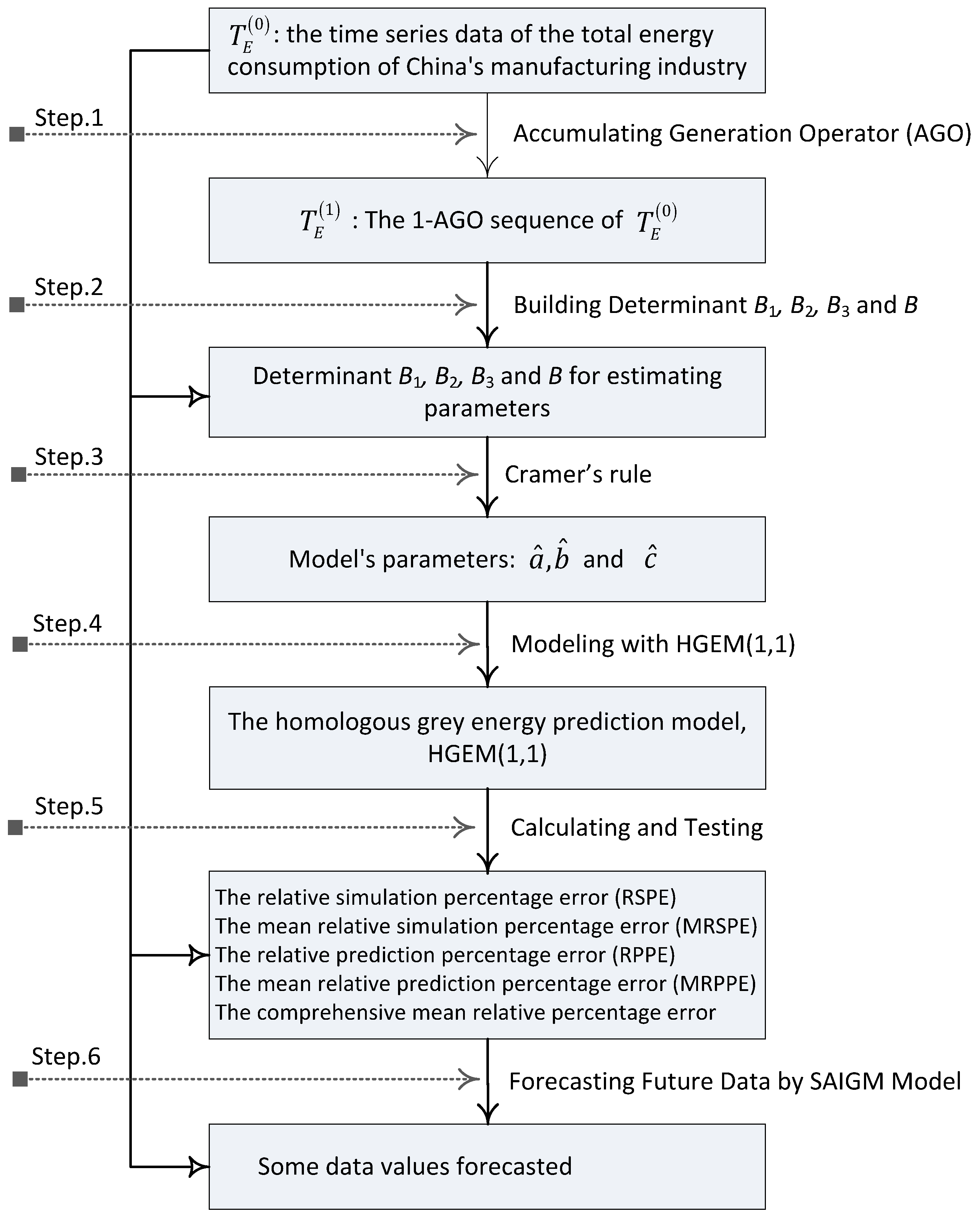
The modelling flowchart of the HGEM(1,1) model can be seen in Figure 1, as follows.
4. Forecasting the Energy Consumption of China’s Manufacturing with HGEM(1,1)
In recent years, China’s manufacturing industry has risen rapidly and has become a major manufacturing country in the world. However, the development of the manufacturing industry is mainly based on the consumption of large amounts of coal, petroleum and other non-renewable energy sources, which results in an energy shortage in China. China’s manufacturing industry consumes 54% of China’s total energy consumption. Hence, it is of great theoretical and practical significance to forecast the energy consumption situation of China’s manufacturing industry in the future. Such a forecast would be instrumental to ensuring the effective supply of energy in China’s manufacturing industry and promote the sustainable development of China’s economy. The energy consumptions of China’s manufacturing (CMEC) during 2006–2012 are as shown in Table 1, as follows.
From Table 1
Data are applied to build the HGEM(1,1) model of the energy consumption of China’s manufacturing; and the last data is used to check the prediction performance of the HGEM(1,1) model.
The detailed modelling process of the HGEM(1,1) model contains four steps, which are parameter estimation, model construction, model performance test and data prediction, as follows.
Step 1 Parameter estimation
From Definition 2.1,
Constructing determinants from , the parameters of the HGEM(1,1) can be estimated by Cramer’s rule as follows:
That is
Step 2 Model construction
Substituting into Equation (2), we can obtain
Then
Equation (17) is just the HGEM(1,1) model for forecasting the energy consumption of China’s manufacturing.
Step 3 Model performance comparisons and tests
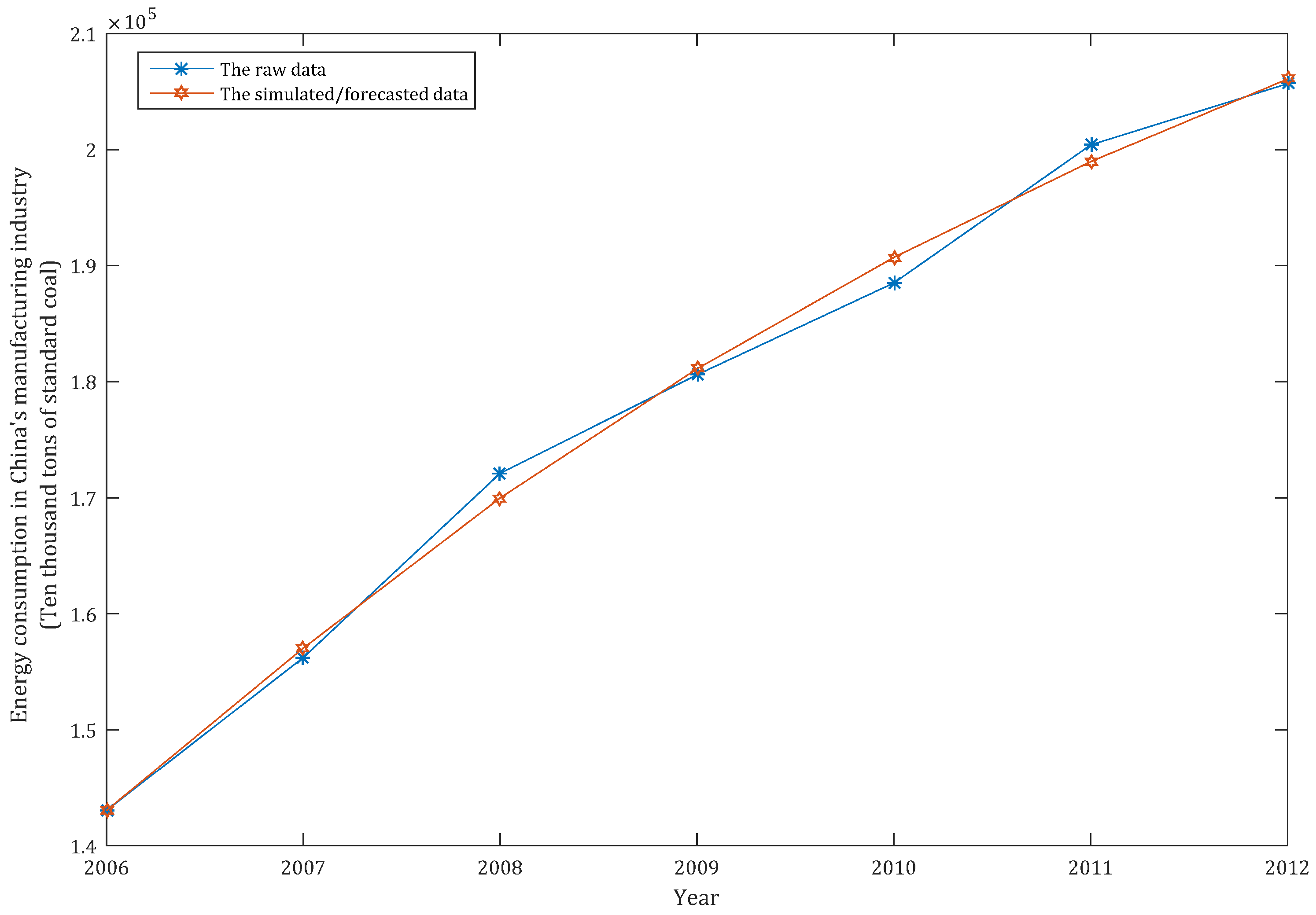
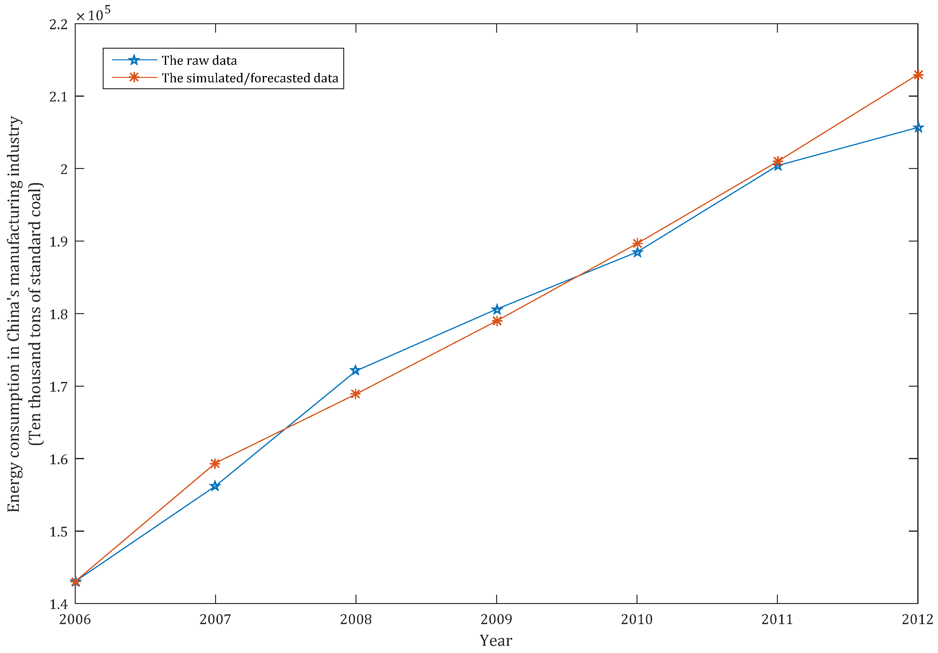
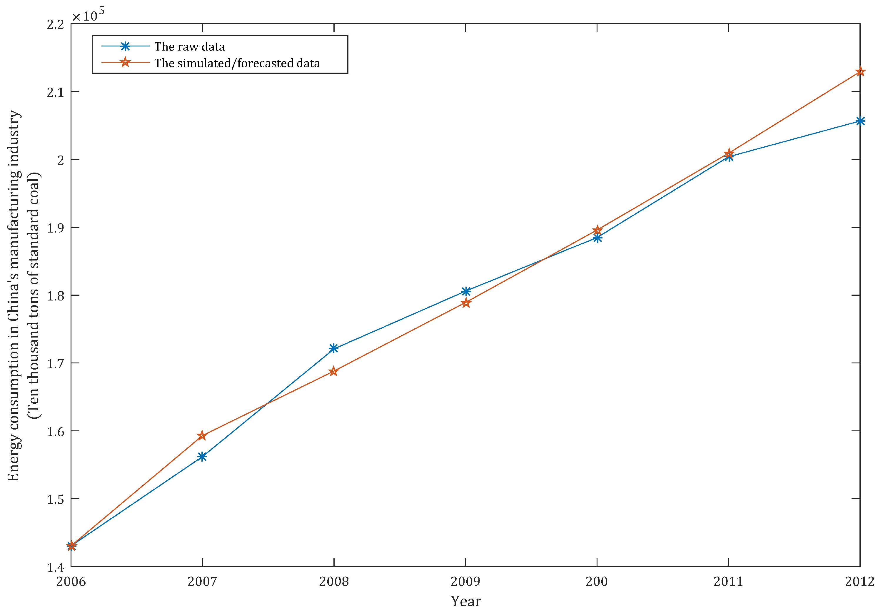
When , we can simulate the energy consumption of China’s manufacturing; when , the energy consumption of China’s manufacturing can be forecast. In order to compare the simulation and prediction performance of the HGEM(1,1), we also apply the classic GM(1,1) model and the frequently-used DGM(1,1) model to simulate and forecast the energy consumption of China’s manufacturing industry. All the simulation and prediction results of the above three models are shown in Table 2, as follows:
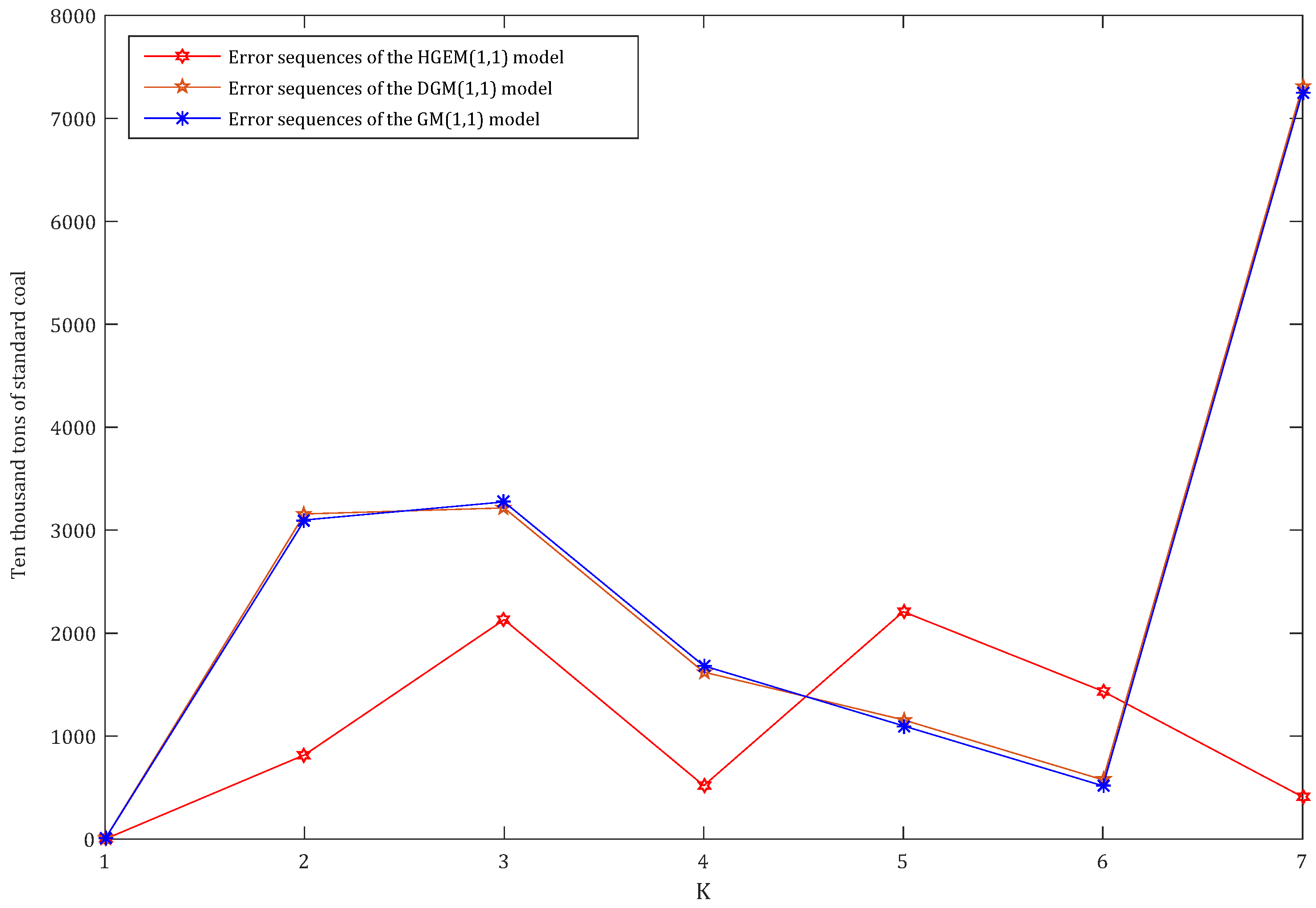
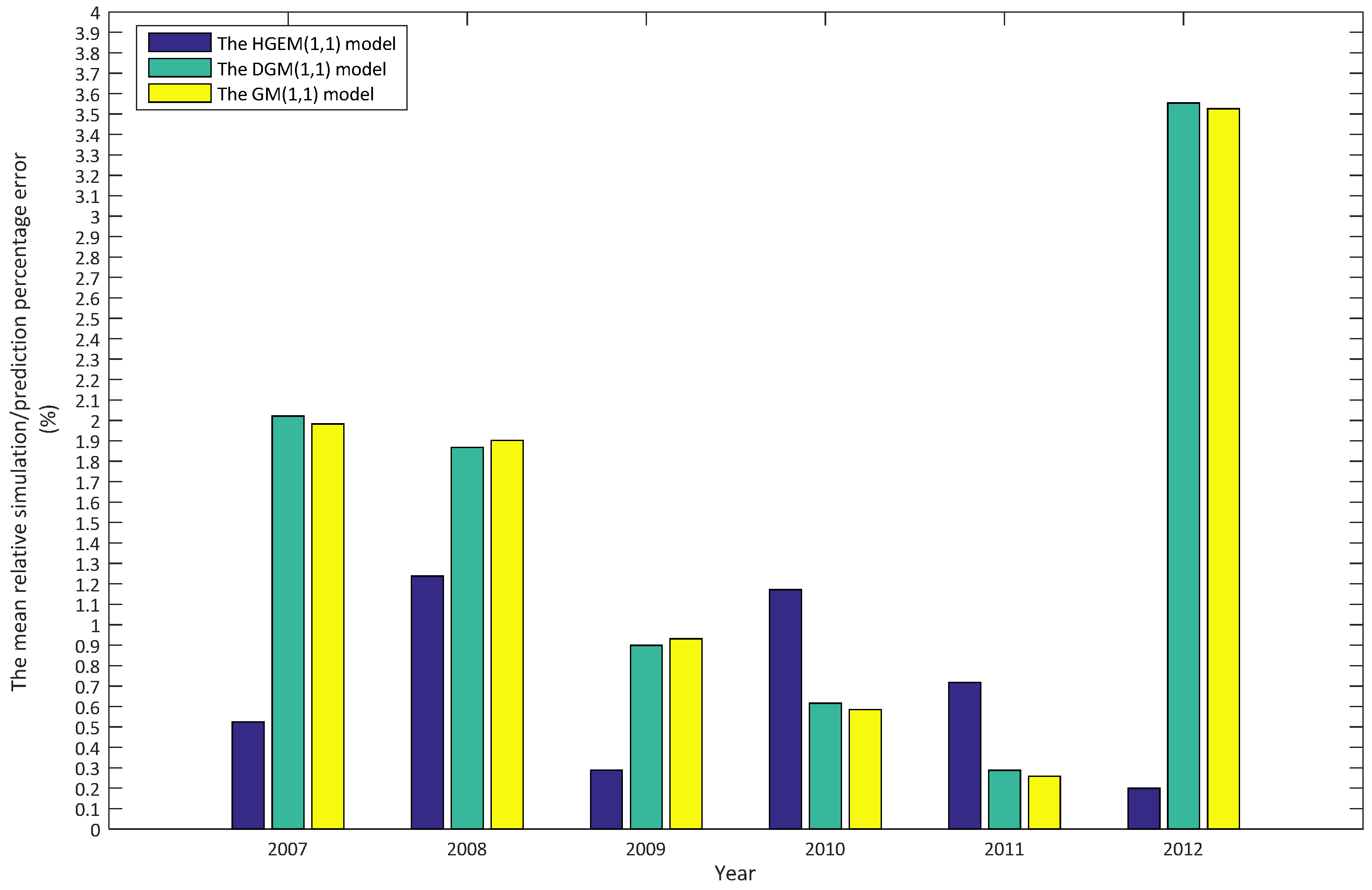
Table 2 shows the HGEM(1,1) model to be better than the DGM(1,1) and GM(1,1) models in both simulation and prediction accuracy. In order to clearly compare the performance of the three models, we drew the simulation and prediction curves and errors of the three models based on the data in Table 2 in MATLAB, as shown in Figure 2, Figure 3, Figure 4, Figure 5 and Figure 6, as follows.
According to Figure 2, Figure 3, Figure 4, Figure 5 and Figure 6, the performances of the simulation and prediction of the HGEM(1,1) model are the best among the above three models, and those of the DGM(1,1) model and the GM(1,1) model are very close to each other. By checking the grey model error level reference table, we can see that the comprehensive grade of the HGEM(1,1) model is I, which can be used for prediction.
Step 4 Prediction
According to Equation (17), the total energy consumption of China’s manufacturing industry in the next 2018–2024 years can be predicted, as shown in Table 3.
From Table 3, we can see that the total energy consumption of China’s manufacturing industry will slow down during 2018–2024, but the total amount is still too large. In order to ensure the effective supply of China’s manufacturing energy, and promote the sustainable development of China’s economy, some countermeasures and suggestions are put forward in Section 5.
From Table 2, the out-of-sample data is only one, and it is difficult to test the prediction performance of the HGEM(1,1) model usefully. To this end, we adjusted the proportion of in-sample and out-of-sample and built a new HGEM(1,1) model, HGEM(1,1)II to simulate and forecast the energy consumption of China’s manufacturing. The parameters of HGEM(1,1)II are shown in Table 4, as follows.
We built the HGEM(1,1)II model with the parameters in Table 4, and the simulation and prediction results of the HGEM(1,1)II model are shown in Table 5, as follows:
It is obvious from Table 2 and Table 5 that the comprehensive mean relative percentage error (CMRPE) of the HGEM(1,1) model is only 0.494%, which is better than that of the other seven models. Therefore, it is reliable and reasonable that we apply the HGEM(1,1) model to forecast the energy consumption of China’s manufacturing (CMEC) during 2013–2024.
5. Suggestions
By 2024, the energy consumption of China’s manufacturing will be as high as 242824.144 ten thousand tons of standard coal, which accounts for approximately 60% of China’s total energy consumption in 2016 according to Table 3. Therefore, it is a major concern of China’s government that some measures need to be taken to control the energy consumption of China’s manufacturing industry. In order to control the high energy consumption of China’s manufacturing industry, the main measures are to optimize the industrial structure, speed up the elimination of backward production capacity, and promote the transformation and upgrading of traditional industries. After this, the green development of the manufacturing industry can be achieved.
First, it should adjust and optimize China’s manufacturing structure. The excessive growth trend of high energy consumption and pollution industries need be controlled. Some policies and measures to promote industrial restructuring should be improved and should actively promote the adjustment of the energy structure in China’s manufacturing industry. Meanwhile, we should formulate policies and measures to promote the development of high-tech industries. Secondly, we will eliminate backward production capacity and control the development of ‘two high’ industries which are highly polluting and high energy consuming enterprises. China’s government should eliminate backward technology, technology and equipment in small and medium-sized enterprises, especially high energy consumption and heavy pollution industries, such as iron and steel, nonferrous metals, chemicals, building materials, power and other industries. China’s government departments should eliminate “two high” and “five small” enterprises and the backward production capacity of enterprises be in accordance with the relevant requirements, step by step. Thirdly, they should speed up energy-saving emission reduction technology development and generalization, and promote the development of a circular economy. In view of the characteristics of small and medium-sized enterprises, we will speed up the development of common, key and cutting-edge energy-saving emission reduction technologies, and foster a technological innovation system of energy saving and emission reduction, which combines enterprises as the main body and combines production, production and research, and speeds up the transformation of scientific and technological achievements. A variety of methods are used to speed up the promotion and application of the efficient energy-saving new technologies, new processes, new products and new equipment.
6. Conclusions
China is the largest manufacturing energy consuming country in the world. Energy supply and price are the two key factors that influence the sustainable development of China’s manufacturing industry. Hence, a scientific prediction of the total energy consumption of China’s manufacturing industry has a positive significance on the smooth and healthy development of China’s manufacturing industry. To this end, the HGEM(1,1) model specially used for energy prediction was constructed, and we studied the parameter estimation method, time response formula and performance test method of the new model. Finally, the HGEM(1,1) model was applied to simulate and forecast the energy of China’s manufacturing industry, and corresponding countermeasures and suggestions were put forward according to the prediction results.
Optimizing the initial value, background value and accumulating order of the HGEM(1,1) model, and then constructing a better grey prediction model of total energy consumption are the next research target of our team.
Acknowledgments
Our work was supported by National Natural Science Foundation of China (71771033, 71271226), Chongqing Municipal Social Science Planning Commission Project of China (2016WT37), Science and technology research project of Chongqing Education Commission (KJ1706166) and the open research fund of Chongqing Key Laboratory of Electronic Commerce & Supply Chain System (1456026). We would like to thank the anonymous referees for their constructive comments that helped to improve the clarity and completeness of this paper.
Author Contributions
Bo Zeng conceived and designed the study. Meng Zhou performed the modeling process and error checking methods for the HGEM(1,1) model. Jun Zhang provided the MATLAB code with HGEM(1,1) and performed the calculations of Section 4. All authors read and approved the manuscript.
Conflicts of Interest
The authors declare no conflict of interest.
References
- Wu, J.; Mohamed, R.; Wang, Z.; Wu, J.; Mohamed, R.; Wang, Z. An agent-based model to project China’s energy consumption and carbon emission peaks at multiple levels. Sustainability 2017, 9, 893. [Google Scholar] [CrossRef]
- Liu, P.; Zhou, Y.; Zhou, D.K.; Xue, L. Energy performance contract models for the diffusion of green-manufacturing technologies in China: A stakeholder analysis from SMEs’ perspective. Energy Policy 2017, 106, 59–67. [Google Scholar] [CrossRef]
- Wan, Z. Analysis of economic growth and energy consumption of China’s manufacturing industry. East China Sci. Technol. Acad. Ed. 2015, 3, 421. (In Chinese) [Google Scholar]
- Sun, W.; Ji, S.S. Research on the Energy Consumption Index of Manufacturing Based on Maximum Deviation. Sci. Technol. Manag. Res. 2016, 354, 233–239. (In Chinese) [Google Scholar]
- Hou, J.; Chen, H.; Xu, J. External knowledge sourcing and green innovation growth with environmental and energy regulations: Evidence from manufacturing in China. Sustainability 2017, 9, 342. [Google Scholar] [CrossRef]
- Pan, H.; Zhang, H.; Zhang, X. China’s provincial industrial energy efficiency and its determinants. Math. Comput. Model. 2013, 58, 1032–1039. [Google Scholar]
- Li, K.; Lin, B. Impact of energy conservation policies on the green productivity in China’s manufacturing sector: Evidence from a three-stage dea model. Appl. Energy 2016, 168, 351–363. [Google Scholar] [CrossRef]
- Yang, M.; Yang, F. Energy-efficiency policies and energy productivity improvements: Evidence from China’s manufacturing industry. Emerg. Mark. Financ. Trade 2016, 52, 1395–1404. [Google Scholar] [CrossRef]
- Zhu, J.; Ruth, M. Relocation or reallocation: Impacts of differentiated energy saving regulation on manufacturing industries in China. Ecol. Econ. 2015, 110, 119–133. [Google Scholar] [CrossRef]
- Wang, Z.X.; Zheng, H.H.; Pei, L.L.; Jin, T. Decomposition of the factors influencing export fluctuation in China’s new energy industry based on a constant market share model. Energy Policy 2017, 109, 22–35. [Google Scholar] [CrossRef]
- Qu, Y.; Yu, Y.; Appolloni, A.; Li, M.R.; Liu, Y. Measuring Green Growth Efficiency for Chinese Manufacturing Industries. Sustainability 2017, 9, 637. [Google Scholar] [CrossRef]
- Chen, X.; Gong, Z.W. DEA Efficiency of Energy Consumption in China’s Manufacturing Sectors with Environmental Regulation Policy Constraints. Sustainability 2017, 9, 210. [Google Scholar] [CrossRef]
- Lin, B.; Liu, W. Scenario Prediction of Energy Consumption and CO2 Emissions in China’s Machinery Industry. Sustainability 2017, 9, 87. [Google Scholar] [CrossRef]
- Liu, S.F.; Forrest, J.; Yang, Y.J. A brief introduction to grey systems theory. Grey Syst. Theory Appl. 2012, 2, 89–104. [Google Scholar] [CrossRef]
- Helaleh, A.H.; Alizadeh, M. Performance prediction model of miscible surfactant-CO2, displacement in porous media using support vector machine regression with parameters selected by ant colony optimization. J. Nat. Gas Sci. Eng. 2016, 30, 388–404. [Google Scholar] [CrossRef]
- Lakshmanan, G.T.; Shamsi, D.; Doganata, Y.N.; Unuvar, M.; Khalaf, R. A markov prediction model for data-driven semi-structured business processes. Knowl. Inf. Syst. 2015, 42, 97–126. [Google Scholar] [CrossRef]
- Chae, Y.T.; Horesh, R.; Hwang, Y.; Lee, Y.M. Artificial neural network model for forecasting sub-hourly electricity usage in commercial buildings. Energy Build. 2016, 111, 184–194. [Google Scholar] [CrossRef]
- Deng, J.L. The Control problem of grey systems. Syst. Control Lett. 1982, 1, 288–294. [Google Scholar]
- Liu, S.F.; Lin, Y. Grey Systems Theory and Applications; Springer-Verlag: Berlin/Heidelberg, Germany, 2010. [Google Scholar]
- Zeng, B.; Chen, G.; Liu, S.F. A novel interval grey prediction model considering uncertain information. J. Frankl. Inst. 2013, 350, 3400–3416. [Google Scholar] [CrossRef]
- Li, C.; Cabrera, D.; de Oliveira, J.V.; Sanchez, R.V.; Cerrada, M.; Zurita, G. Extracting repetitive transients for rotating machinery diagnosis using multiscale clustered grey infogram. Mech. Syst. Signal Process. 2016, 76–77, 157–173. [Google Scholar] [CrossRef]
- Wang, Z.X.; Li, Q.; Pei, L.L. Grey forecasting method of quarterly hydropower production in China based on a data grouping approach. Appl. Math. Model. 2017, 51, 302–316. [Google Scholar] [CrossRef]
- Wang, Y.H.; Dang, Y.G.; Li, Y.Q.; Liu, S.F. An approach to increase prediction precise of GM(1,1) model based on optimization of the initial condition. Expert Syst. Appl. 2010, 37, 5640–5644. [Google Scholar] [CrossRef]
- Zeng, B.; Li, C.; Long, X.J. Equivalency and unbiasedness of grey prediction models. J. Syst. Eng. Electron. 2015, 26, 110–118. [Google Scholar] [CrossRef]
- Zeng, B.; Meng, W.; Tong, M.Y. A self-adaptive intelligence grey predictive model with alterable structure and its application. Eng. Appl. Artif. Intell. 2016, 50, 236–244. [Google Scholar] [CrossRef]
- Xie, N.M.; Liu, S.F.; Yang, Y.J.; Yuan, C.Q. On novel grey forecasting model based on non-homogeneous index sequence. Appl. Math. Model. 2013, 37, 5059–5068. [Google Scholar] [CrossRef]
- Zeng, B.; Meng, W.; Liu, S.F. Research on prediction model of oscillatory sequence based on GM(1,1) and its application in electricity demand prediction. J. Grey Syst. 2013, 25, 31–40. [Google Scholar]
- Zeng, B. Forecasting the relation of supply and demand of natural gas in China during 2015–2020 using a novel grey model. J. Intell. Fuzzy Syst. 2017, 32, 141–155. [Google Scholar] [CrossRef]
Figure 1.
The modelling flowchart of the HGEM(1,1) model.

Figure 2.
The simulated/forecast curve of the HGEM(1,1) model.

Figure 3.
The simulated/forecast curve of the DGM(1,1) model.

Figure 4.
The simulated/forecast curve of the GM(1,1) model.

Figure 5.
The errors of simulated/forecast curve of HGEM(1,1), DGM(1,1) and GM(1,1).

Figure 6.
The mean relative simulation/prediction percentage error of HGEM(1,1), DGM(1,1) and GM(1,1).
Figure 6.
The mean relative simulation/prediction percentage error of HGEM(1,1), DGM(1,1) and GM(1,1).


Table 1.
The energy consumption of China’s manufacturing (CMEC) during 2006–2012.
| Year | 2006 | 2007 | 2008 | 2009 | 2010 | 2011 | 2012 |
|---|---|---|---|---|---|---|---|
| 1 | 2 | 3 | 4 | 5 | 6 | 7 | |
| CMEC | 143,051.46 | 156,218.80 | 172,106.52 | 180,595.96 | 188,497.85 | 200,403.37 | 205,667.69 |
Unit: Ten thousand tons of standard coal.
Table 2.
Simulated/forecast values and errors of HEGM(1,1), DGM(1,1) and GM(1,1).
| Serial Number | Raw Data | Model HGEM(1,1) | Model DGM(1,1) | Model GM(1,1) | ||||||
| 1 | 143,051.46 | 143,051.460 | 0.000 | 0.000% | 143,051.46 | 0.000 | 0.000% | 143,051.46 | 0.000 | 0.000% |
| 2 | 156,218.80 | 157,037.777 | 818.977 | 0.524% | 159,377.078 | 3158.278 | 2.022% | 159,317.044 | 3098.244 | 1.983% |
| 3 | 172,106.52 | 169,975.742 | 2130.778 | 1.238% | 168,891.070 | 3215.450 | 1.868% | 168,831.317 | 3275.203 | 1.903% |
| 4 | 180,595.96 | 181,115.803 | 519.843 | 0.288% | 178,972.998 | 1622.962 | 0.899% | 178,913.774 | 1682.186 | 0.931% |
| 5 | 188,497.85 | 190,707.802 | 2209.952 | 1.172% | 189,656.766 | 1158.916 | 0.615% | 189,598.346 | 1100.496 | 0.584% |
| 6 | 200,403.37 | 198,966.863 | 1436.507 | 0.717% | 200,978.299 | 574.9290 | 0.287% | 200,920.991 | 517.621 | 0.258% |
| MRSPE () | 0.788% | 1.138% | 1.132% | |||||||
| In-Sample (Simulated Data) | ||||||||||
| 7 | 205,667.69 | 206,078.217 | 410.527 | 0.199% | 212,975.669 | 7307.979 | 3.553% | 212,919.815 | 7252.125 | 3.526% |
| MRFPE () | 0.199% | 4.572% | 4.570% | |||||||
| Out-of-Sample (Forecast Data) | ||||||||||
| CMRPE() | 0.494% | 2.855% | 2.851% | |||||||
Table 3.
Prediction data of the energy consumption of China’s manufacturing (CMEC) during 2013–2024.
Table 3.
Prediction data of the energy consumption of China’s manufacturing (CMEC) during 2013–2024.
| Year | CMEC | Year | CMEC | Year | CMEC | Year | CMEC |
|---|---|---|---|---|---|---|---|
| 2013 | 212,201.352 | 2016 | 225,921.945 | 2019 | 234,680.604 | 2022 | 240,271.769 |
| 2014 | 217,473.595 | 2017 | 229,287.527 | 2020 | 236,829.052 | 2023 | 241,643.249 |
| 2015 | 222,013.189 | 2018 | 232,185.415 | 2021 | 238,678.944 | 2024 | 242,824.144 |
Unit: Ten thousand tons of standard coal.
Table 4.
Value of the parameters of the HGEM(1,1)II model.
| Parameter | ||||||
|---|---|---|---|---|---|---|
| Value | 0.661679 | 68,008.995930 | 68,748.127136 | 0.661679 | 68,008.995930 | 68,748.127136 |
Table 5.
Simulated/forecast values and errors of HEGM(1,1)II, DGM(1,1) and GM(1,1).
| Serial Number | Raw Data | Model HGEM(1,1) II | Model GM(1,1) II | Model DGM(1,1) II | ||||||
| 1 | 143,051.46 | 143,051.460 | 0.000 | 0.000% | 143,051.46 | 0.000 | 0.000% | 143,051.46 | 0.000 | 0.000% |
| 2 | 156,218.80 | 156,368.819 | 150.019 | 0.096% | 158,990.838 | −2772.038 | 1.774% | 159,060.695 | 2841.895 | 1.819 |
| 3 | 172,106.52 | 171,474.973 | −631.547 | 0.367% | 168,791.717 | 3314.803 | 1.926% | 168,855.452 | −3251.068 | 1.889 |
| 4 | 180,595.96 | 181,470.400 | 874.44 | 0.484% | 179,196.764 | 1399.196 | 0.775% | 179,253.359 | −1342.601 | 0.743 |
| 5 | 188,497.85 | 188,497.850 | 150.019 | 0.096% | 190,243.223 | −1745.373 | 0.926% | 190,291.556 | 1793.706 | 0.952 |
| MRSPE () | 0.237% | 1.350% | 1.351% | |||||||
| In-Sample (Simulated Data) | ||||||||||
| 6 | 200,403.37 | 192,460.354 | −7943.016 | 3.964% | 201,970.633 | 1567.263 | 0.782% | 202,009.471 | 1606.101 | 0.801% |
| 7 | 205,667.69 | 195,355.988 | −10,311.702 | 5.014% | 214,420.971 | 8753.281 | 4.256% | 214,448.961 | 8781.271 | 4.270% |
| MRFPE () | 4.489% | 2.519% | 2.536% | |||||||
| Out-of-Sample (Forecast Data) | ||||||||||
| CMRPE() | 2.564% | 1.935% | 1.944% | |||||||
© 2017 by the authors. Licensee MDPI, Basel, Switzerland. This article is an open access article distributed under the terms and conditions of the Creative Commons Attribution (CC BY) license (http://creativecommons.org/licenses/by/4.0/).
Share and Cite
MDPI and ACS Style
Zeng, B.; Zhou, M.; Zhang, J. Forecasting the Energy Consumption of China’s Manufacturing Using a Homologous Grey Prediction Model. Sustainability 2017, 9, 1975. https://0-doi-org.brum.beds.ac.uk/10.3390/su9111975
AMA Style
Zeng B, Zhou M, Zhang J. Forecasting the Energy Consumption of China’s Manufacturing Using a Homologous Grey Prediction Model. Sustainability. 2017; 9(11):1975. https://0-doi-org.brum.beds.ac.uk/10.3390/su9111975
Chicago/Turabian StyleZeng, Bo, Meng Zhou, and Jun Zhang. 2017. "Forecasting the Energy Consumption of China’s Manufacturing Using a Homologous Grey Prediction Model" Sustainability 9, no. 11: 1975. https://0-doi-org.brum.beds.ac.uk/10.3390/su9111975
Note that from the first issue of 2016, this journal uses article numbers instead of page numbers. See further details here.