Circuity Characteristics of Urban Travel Based on GPS Data: A Case Study of Guangzhou

School of Geography and Planning, Sun Yat-Sen University, Guangzhou 510275, China
*
Author to whom correspondence should be addressed.
Sustainability 2017, 9(11), 2156; https://0-doi-org.brum.beds.ac.uk/10.3390/su9112156
Submission received: 11 September 2017
/
Revised: 8 November 2017
/
Accepted: 18 November 2017
/
Published: 22 November 2017
(This article belongs to the Special Issue Neo-Geography and Crowdsourcing Technologies for Sustainable Urban Transportation)
Abstract
:A longer, wider and more complicated change in the travel path is put forward to adapt to the rapidly increasing expansion of metropolises in the field of urban travel. Urban travel requires higher levels of sustainable urban transport. Therefore,this paper explores the circuity characteristics of urban travel and investigates the temporal relationship between time and travel circuity and the spatial relationship between distance and travel circuity to understand the efficiency of urban travel. Based on Guangzhou Taxi-GPS big data, travel circuity is considered in this paper to analyze the circuity spatial distribution and strength characteristics of urban travel in three types of metropolitan regions, including core areas, transition areas and fringe areas. Depending on the different attributes of the three types, the consistency and dissimilar characteristics of travel circuity and influencing factors of travel circuity in metropolises are discussed. The results are shown as follows: (1) by observing the temporal andspatial distribution of travel circuity, it can be found that peaks and troughs change with time, and travel circuity of transition areas is higher than other areas during the peak period. When travelling in these three regions, travel circuity spatial distribution is consistent, which is the core-periphery distribution. When travelling among these three regions, travel circuity spatial distribution is distinct; (2) by analyzing the relationship between time and distance of travel and travel circuity, it can be seen that the shorter the travel time or travel distance, the greater the travel circuity, resulting in a lower travel efficiency; (3) the influence of six factors, including population, road and public transportation, on travel circuity is significant. Whether it is the origin point or destination point, when its location is closer to the city center and the station density of grid is lower, the travel circuity is higher.
1. Introduction
Urban travel is the most important component for higher transport efficiency of a metropolis. However, with thedevelopment of cities, the pressure of sustainable transportation in urban areas is particularly serious. Furthermore, urban travel is also the most difficult problem to be resolved for rapidly developing metropolises. The complexity of urban travel is becoming more and more obvious. Levinson and Krizek clearly point out that the residents’ life (and resulting travel) are more complex, and the city travel time and itinerary becomes more complicated [1]. Zegras finds that changes in urban boundary growth might result in shorter urban trips being replaced by longer inter-urban travel [2].
Presently, how to make urban traffic more efficient is becoming more and more important to sustainable urban development. The mobility of the transportation infrastructure is no longer the main goal of urban sustainable transport, and it tends to study improving the efficiency of the travel process. Banister proposes sustainable mobility as a paradigm for the study of urban complexity [3]. Mobility has become the most important index of urban sustainable transport [4]. Starting from Weibull, who points out the measure method of accessibility, Levension puts forward that both accessibility and mobility are the important indexes of traffic efficiency, and they have become one of the focuses of sustainable transportation [5,6,7]. Urban sustainable transport has shifted from focusing on sustainable transport facilities to paying attention to sustainable personal travel.
Travel circuity is the result of the travel of urban residents. The percentage decrease of travel circuity shows that the travel distance/time between Origin–Destination (OD) pairs is closer to the shortest travel distance/time, and it shows that the residents’ travel efficiency will be improved, and that the sustainable development of urban traffic is guaranteed. Travel circuity is influenced by the urban development environment,which plays an important role in measuring urban travel efficiency in the sustainable development of urban transport. Besides, it is conducive to identifying the problems of the travel environment, improving travel efficiency and promoting the sustainable development of urban transport.
Actually, travel circuity and the travel Origin–Destination (OD) point have a close connection. The travel distance between OD pairs depends on the structure of the traffic network and the congestion of the actual road situation within the city [8,9]. The distance between OD pairs has three conditions.Specifically, the first is the Euclidean distance between OD pairs, the second is the road network distance between OD pairs, and the third is the actual path distance between OD pairs [10,11]. Accompanying the development of metropolises, urban sprawl brings urban travel problem that traffic congestion is spreading in the ensuring expansion period. Actual urban travel presents a longer, wider and more complicated change of travel path within the metropolis [12,13]. During the actual urban travel process, the result of travel path choice is not the shortest path in the road network, but the actual travel path after considering the road congestion situation. When the distance between the Euclidean distance and the actual travel path distance is different, travel circuity is formed.
Circuity studies derive from the transport network and travel distance analysis. Circuity is a ratio of the shortest network distance to Euclidean distance between travel Origin–Destination, and it quantifies its deviation from a distance-minimizing straight line in most studies [14,15]. Numerous studies on circuity focus on the analysis of the traffic network circuity, while the travel circuity based on the residents’ travel behavior is seldom involved. Ballou found that the difference between the Euclidean distance and the path distance is referred to as a circuity factor [8]. Depending upon the check for actual travel path circuity based on GPS data, while Wolf found that 58% of trips are high-circuity for suspicious delays. It is an important factor to reflect and evaluate the distance of network travel, and it is often used to assess the structural characteristics of the transport network [11].
Current studies on travel circuity have been carried out that focus on the macro, medium and micro scales, such as the study of traffic network travel circuity on the national scale, the regional scale, and the urban scale. Additionally, regarding the national scale study involved developing countries, other studies have mainly been concentrated on Europe and America, such as by comparing the commuter circuity of 22 cities in the United States and the road network circuity analysis of 51 cities in the United States [8,14,16,17]. The research content of the travel circuity is constantly deepening, and current studies describe the travel circuity mainly from the two dimensions, time and distance, respectively.
These studies are usually concerned with horizontal contrast among different regions or cities, while ignoring the study of different types of travel circuity within the city. Previously, relevant qualitative analysis and quantitative analysis were carried out, yet few travel circuity studies focused on the geographic spatial analysis. Furthermore, the spatial distribution characteristics of travel circuity are important for understanding and interpreting travel behaviors.
With its fast and accurate real-time feedback characteristics, taxi global positioning system (GPS) data is widely used in the field of traffic research in the process of rapid development of information communication technology (ICT). Taxi GPS data used in dynamic traffic assignment, travel time prediction, and path analysis, can be used to reflect the basic reliable data of real traffic situation [18,19,20]. While in the study of path analysis, through the data mining of GPS data,the driving trajectory of the taxi GPS data that can be adopted for the optimization of the travel pathcan be extracted [21].
The purpose of this study is to answer the following three question: (1) What are the characteristics of travel circuity in different urban areas through GPS data analysis? (2) What is the relationship among travel circuity and travel time and travel distance in diverse urban areas? (3) What is the impact of urban environmental factors on travel circuity? Therefore, based on Guangzhou Taxi-GPS data, travel circuity is taken as a perspective in this paper, to analyze the spatial distribution and circuity strength characteristics of travel circuity in three regions of metropolises including core areas, transition areas and fringe areas. According to the distinct attributes of the three regions, the consistency and dissimilar characteristics of travel circuity and influencing factors of travel circuity in metropolises are discussed. This paper takes the actual behavior of urban residents as the basis to study the spatial distribution characteristics and impact relationship of travel circuity, thus providing a new way of thinking for the study of urban residents’ travel efficiency, and promoting urban sustainable transport development.
Currently, with the development of geo-information science, more and more researchers use crowdsourced or volunteered geographic information as their dataset source. Besides, crowdsourced or volunteered geographic information studies on routing and navigation. For example, Hendawi point out the proliferation of volunteered geographic information (VGI) such as GPS tracks donated by individuals via forums such as OpenStreetMap has created an opportunity for providing next generation routing services [22]. Mobasheri proved crowdsourced datasets are suitable for specialized routing services [23]. Graser pointed out that the quality of these data sources and OpenStreetMap, in particular, is sufficient for answering questions about the heterogeneous nature of VGI in general [24]. In addition, crowdsourced or volunteered geographic information was used for urban and environmental studies. Sun conducted an empirical investigation in Chicago with cycling data from a bicycle–sharing systems (BSS) called Divvy. Divvy publicizes cycling trips of BSS users (including both annual members and casual users) with start and end docking stations as well as trip duration. The BSS data was contributed by individual riders, and thus is considered a type of crowdsourced geographic information (CGI) and has high potential for studies of active travel and sustainable transport [25]. Mooney discuss how CGI and VGI can be used as a complement/addition, or in some cases a replacement, to traditionally generated sources of spatial data and information [26]. Crooks addressed the opportunities presented by the emergence of crowdsourced data to gain novel insights into form and function in urban spaces. These data provide a first-hand account of form and function from the people who define urban space through their activities [27]. The GPS data used in the paper could be categorized as crowdsourced data (but not volunteered). Although we used this dataset in our analyses, other sources of GPS traces collected from volunteers could also be used, if available. Therefore, our method is generic in this sense.
The paperis organized as follows: Section 2 defines travel circuity and the calculation method; Section 3 introduces data sources and research areas; the spatial and temporal distribution of travel circuity are explored in Section 4; Section 5 discusses research resultsconcerning the relationship between travel circuity, travel time and travel distance; the influences of urban environment factors on travel circuity are discussed in Section 6, while final section concludeskey findings.
2. Travel Circuity
2.1. Definition
The real travel distance between OD pairs is often greater than the Euclidean distance, in addition to the road network structure. Based on the congestion situation of road, residents’ travel route choice also determines the travel distance.
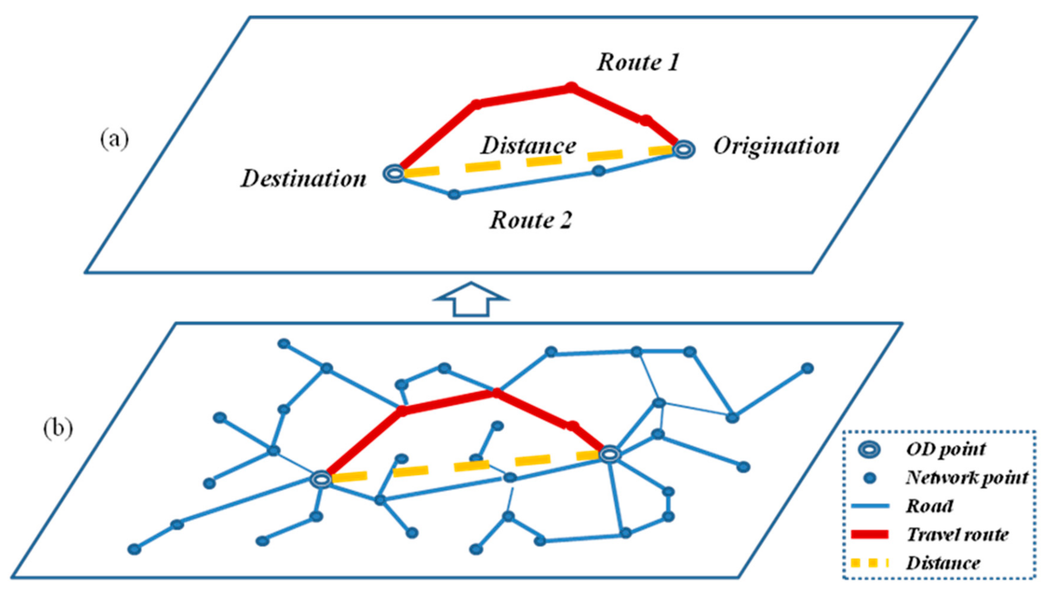
Travel circuity refers to the gap between the actual travel path distance and Euclidean distance between the OD pairs in the travel process. Figure 1 exhibits the travel circuity. The greater the gap, the stronger circuity degree. Travel circuity is closely related to the structure of the road network and the distance of real travel path, which is selected by travelers.The length of the travel is restricted by the structure of the road network, which reflects the difficulty of the urban residents’ travel.
2.2. Method
Circuity is defined as the ratio of the path distance to the Euclidean distance between the travel OD pairs, which is used to explain the travel distance [19]. However, travel circuity is the ratio of the actual travel path distance to the Euclidean distance between the travel OD pairs. Therefore, travel circuity is calculated as:
where is the circuity of a real trip with origin i and destination j (i.e., an OD pair), denotes the Euclidean distance and denotes the real path distance between origin i and destination j. Hence, the theoretical minimal value of circuity is 1 when the shortest network distance equals the Euclidean distance. When the circuity value is closer to 1, then the travel efficiency is higher.
Because the OD pair of taxi GPS data shows random distribution, the data should be turned into grid. To qualify, if the origin and destination of a trip fall into the grid i and the grid j respectively, grid i and grid j are used as travel and , and the OD matrix is constructed for conducting the analysis. Then the average circuity of all O points of GPS data that travel from grid to grid , is regarded as the circuity of the grid . It can be expressed as:
where is the circuity of grid . denotes the number of all O points in grid . denotes the circuity of the nth O points. While is smaller and shows that the smaller the circuity of grid is, the higher the travel efficiency of grid is.
3. Data Sources and Research Area
3.1. Data Sources
3.1.1. Floating Car Data (FCD)
The floating car data (FCD) of this research is obtained from the Guangzhou Fangwei Traffic Science and Technology Co., Ltd., Guangzhou City, China on 1–7 May 2009 for the taxi FCD. According to statistics, the number of floating carsis about 14,000 per day, and the original data of FCD are about 2400 million per day.
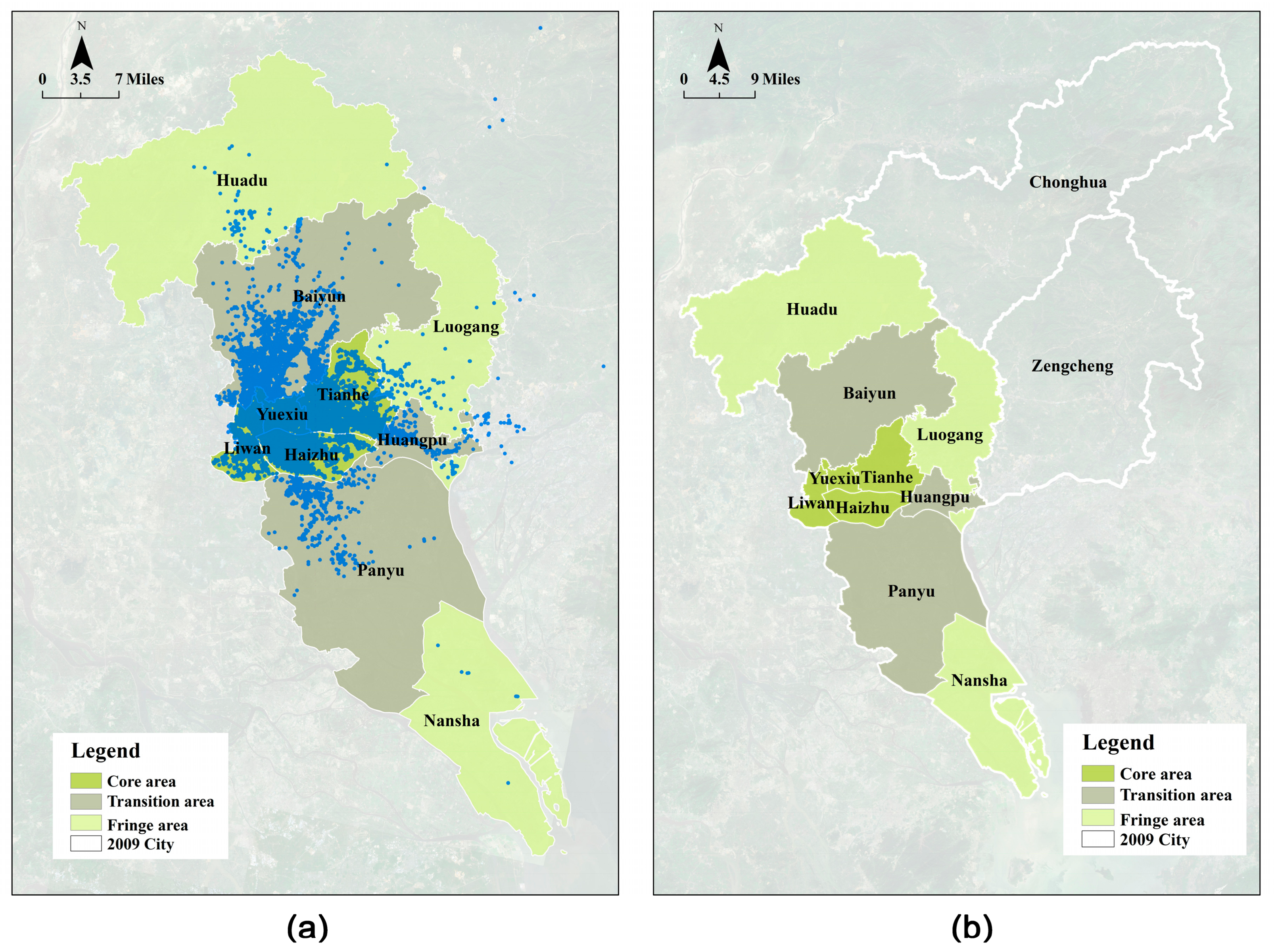
Influenced by the acquisition of hardware and software equipment, the following four types of abnormal data are removed: (1) latitude and longitude data that is beyond the scope of the study area; (2) the travel speed is far greater than the normal speed, when considering the real situation of traffic in Guangzhou and the performance of the taxi, excluding the speed of the data at 100 km/h or more; (3) the validity of data is 0; (4) the abnormal condition of passenger carrying. Abnormal results (3) and (4) are the data that seemed to give the acquisition equipment difficulty, so they were eliminated. Through the OD identification of floating car data, the OD pairs of the taxi are extracted in the passenger carrying status. Besides, the number of valid trips for the taxi is about 52 million times per day. Figure 2 presents a spatial distribution of valid FCD.
The FCD path location data blank is affected by the sampling time interval. This paper uses Wang’s map matching method to deal with path matching [28]. To reduce computational complexity this method mainly considers the following three aspects: (1) It introduces the heading angle variable to emission probability calculation; (2) It divides the road network according to a square grid, and constructs a candidate road segment searching algorithm based on the hash index; (3) Through on preprocessing the road net, it constructs a road segment transition matrix based on the characteristic that floating cars have a limited scope of space activities in the given time, realizing the fast calculation of the road segment transition probability and reducing the time complexity of the road matching calculation.
3.1.2. Urban Environment Data
The urban environment data used in this paper mainly include urban society, structure and public transport data. The population data in the social data comes from the Statistical Yearbook of Guangzhou. Besides, the road network data in urban structure data is from OpenStreetMap, and urban public transport data is obtained through Baidu application program interface (API).
3.2. Research Area
Accompanying the rapid development of urbanization in China, China’s mega-cities ushered in a new opportunity for rapid urban expansion. Guangzhou, as a mega-city along the south-east coast of China, has a booming population and an acceleration of urban sprawl. The population in 2009 was 11.8697 million, with a population growth rate of 6.42%. The urban area changed after the urban administrative division in 2005, expanding from 3718.5 square kilometers to 3843.43 square kilometers. Considered a typical metropolis in China, Guangzhou is facing the problem of travel efficiencyand urban traffic congestion, and the sustainable development of urban transport is suffering a great challenge in the process of urban rapid development.
Research areas in this paper include Yuexiu, Liwan, Haizhu, Tianhe, Baiyun, Huangpu, Nansha, Luogang, Huadou and Panyu. Figure 2 shows the ten districts of the research areas. The areas amount to 3843.43 km2. The divisions of regional types are carried out by the highway of Guangzhou. The core areas are four old towns of Guangzhou, namely Yuexiu, Tianhe, Liwan and Haizhu. The transition areas revolve around the core areas, involving Baiyun, Panyu and Whampoa. The fringe areas are located at the edge of the city, containing Luogang, Huadu and Nansha.
4. The Spatial and Temporal Distribution of Travel Circuity
The direct correlation of the travel distance and the travel circuity was subsequently investigated. The degree of travel circuity for taxi passengers was reflected by the FCD data. This study assessed the characteristics of the spatial distribution of travel circuity and the characteristics of relationship with distance respectively from three scales. The first scale mainly focused on the whole research area. The second scale cared about three regions of metropolises, which included core areas, transition areas and fringe areas. The final scale concerned the districts of each regions. Two kinds of software helped us to analyze spatial and temporal distribution of travel circuity. Arcgis10.2 was applied for FCD data visualization. The spatial correlation method of overlay analysis tools was used for spatial analysis of travel circuity. Matlab2010 was applied to carry on the statistical quantification analysis for the travel circuity characteristic.
4.1. Spatial Distribution of Travel Circuity
4.1.1. The Spatial Distribution of Travel Circuity for O Points Showed Uneven Circle and D Points Presented the Even Circle in the Whole Research Area
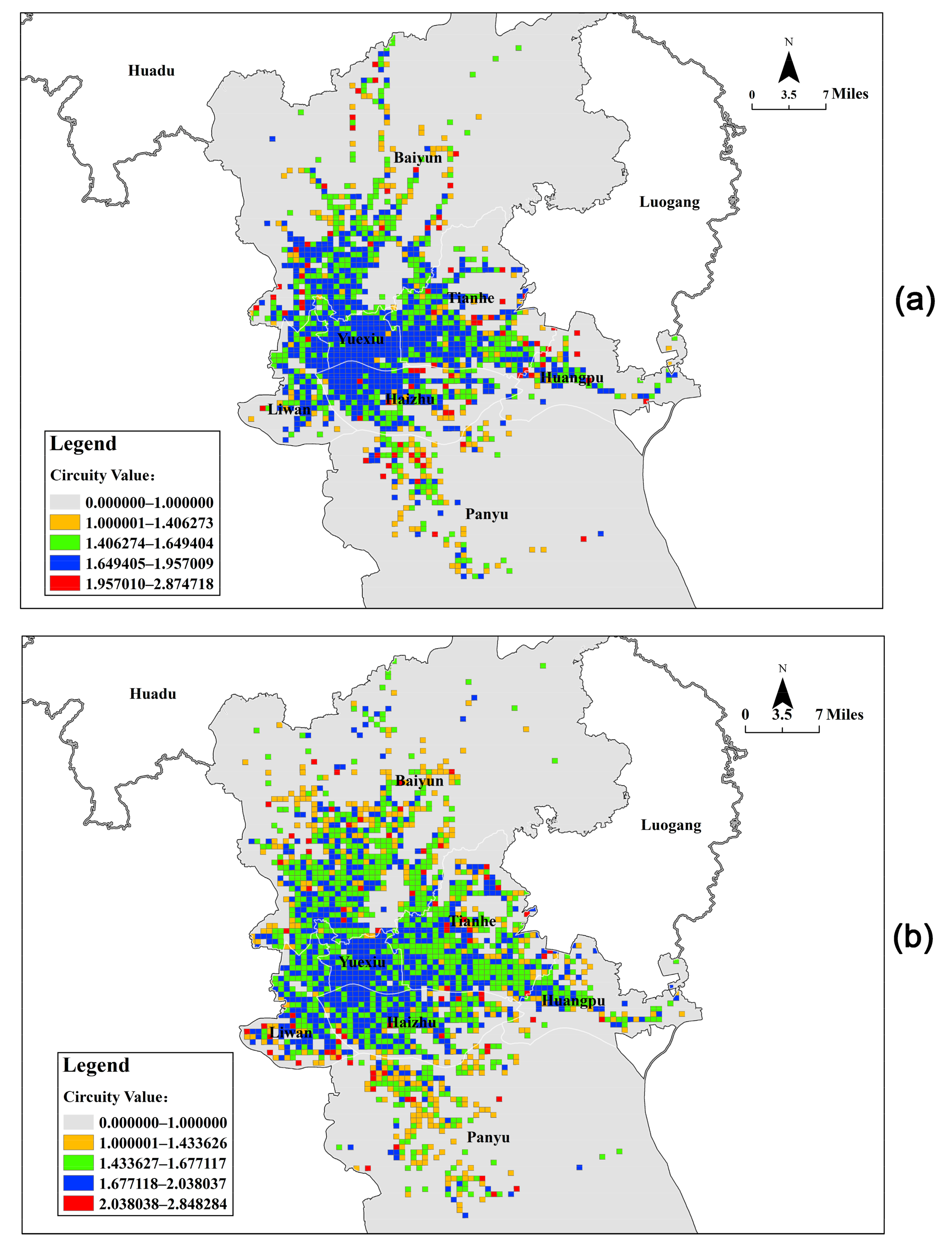
To better comprehend the spatial distribution of travel circuity, research areas were shown in Arcgis10.2. Spatial overlay analysis was used to acquire the O point and D point of each grid that was 100 × 100 m. Consequently, this paper estimated the average value of travel circuity of point O and point D which belonged to each grid. Using the first scale, one can find out that the range of distribution of O points distribution was less than D points for the whole urban travel in Figure 3. The O points of trips were distributed in the core area mainly, while D points of trips were not only distributed in the core area, but also in the transition region. It should be noticed that the distribution range of D points in the transition region was higher than O points.
Travel circuity of OD points is divided into different levels by natural fracture method. It can be found that travel circuity of O point in the core area was concentrated between 1.66 and 1.95, which is the first circle. The second circle was concentrated between 1.46 and 1.65 outward from the center. The circuity of the third circle was concentrated between 1 and 1.45. It is necessary to point out that the circuity of the first circle is not the highest. The travel circuity of the fourth circle around urban edge was the highest, and its value was greater than 1.95. The circuity of O points in the first circle had a wide distribution range, while shrinking in the other circles, and apparent characteristics of the uneven distribution are based on the result of the circuity descending from the centre.
Additionally, travel circuity of D points also presented circle types of the spatial distribution. The circuity of the center circle was in the range of 1.66–2.0. The second circle was in the range of 1.46–1.65. The third circle was in the range of 1–1.45. The value of travel circuity was higher than 2.0 in the fourth circle. The circuity of D points was greater than that of O points in the center and the fourth circle. The circle distribution ranges of D points presented an even uniform circle distribution.
4.1.2. Different Spatial and Intensive Distribution of Travel Circuity for O and D Points among Three Types Regions Are Presented
Travel circuity of O points between core area and transition area presented a zonal cross distribution. The strength of circuity showed a ‘center strong–periphery weak’ distribution characteristic. However, travel circuity of D points between the core area and transition area demonstrated an even distribution in a circle. The strength of circuity appeared as a ‘center weak–periphery strong’ distribution characteristic. Figure 4 illustrates the distribution of travel circuity for OD points between the core area and transition area.
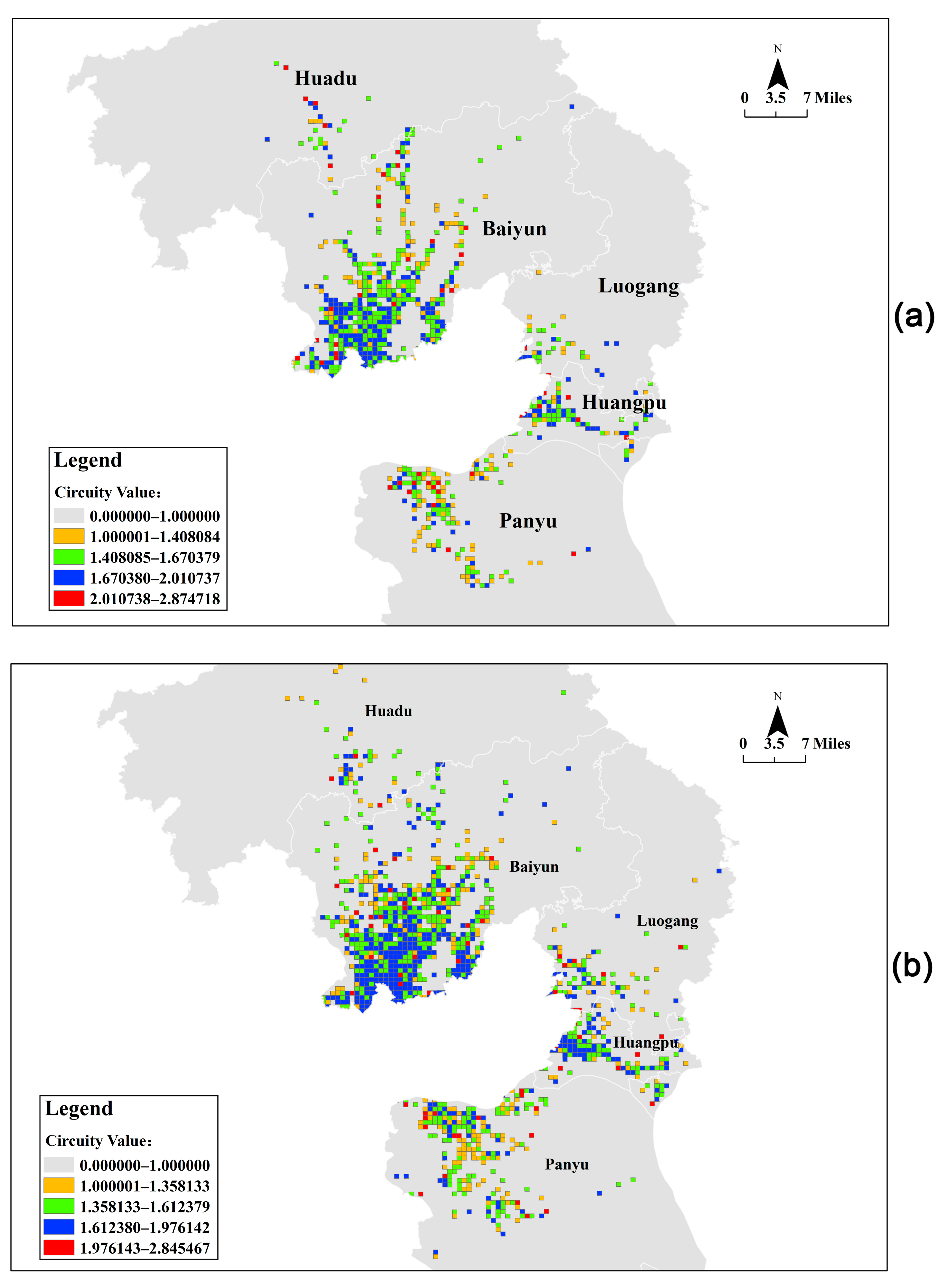
The next step in the analysis is the estimation of travel circuity for O points between the transition area and the fringe area. Travel circuity presented a zonal distribution. The strength of circuity showed a ‘near strong–far weak’ distribution characteristic. Travel circuity of D points between the transition area and the fringe area showed a circle distribution. The strength of circuity exhibited a ‘center strong–periphery weak’ distribution characteristic. Figure 5 presents the distribution of travel circuity for OD points between the transition area and the fringe area.
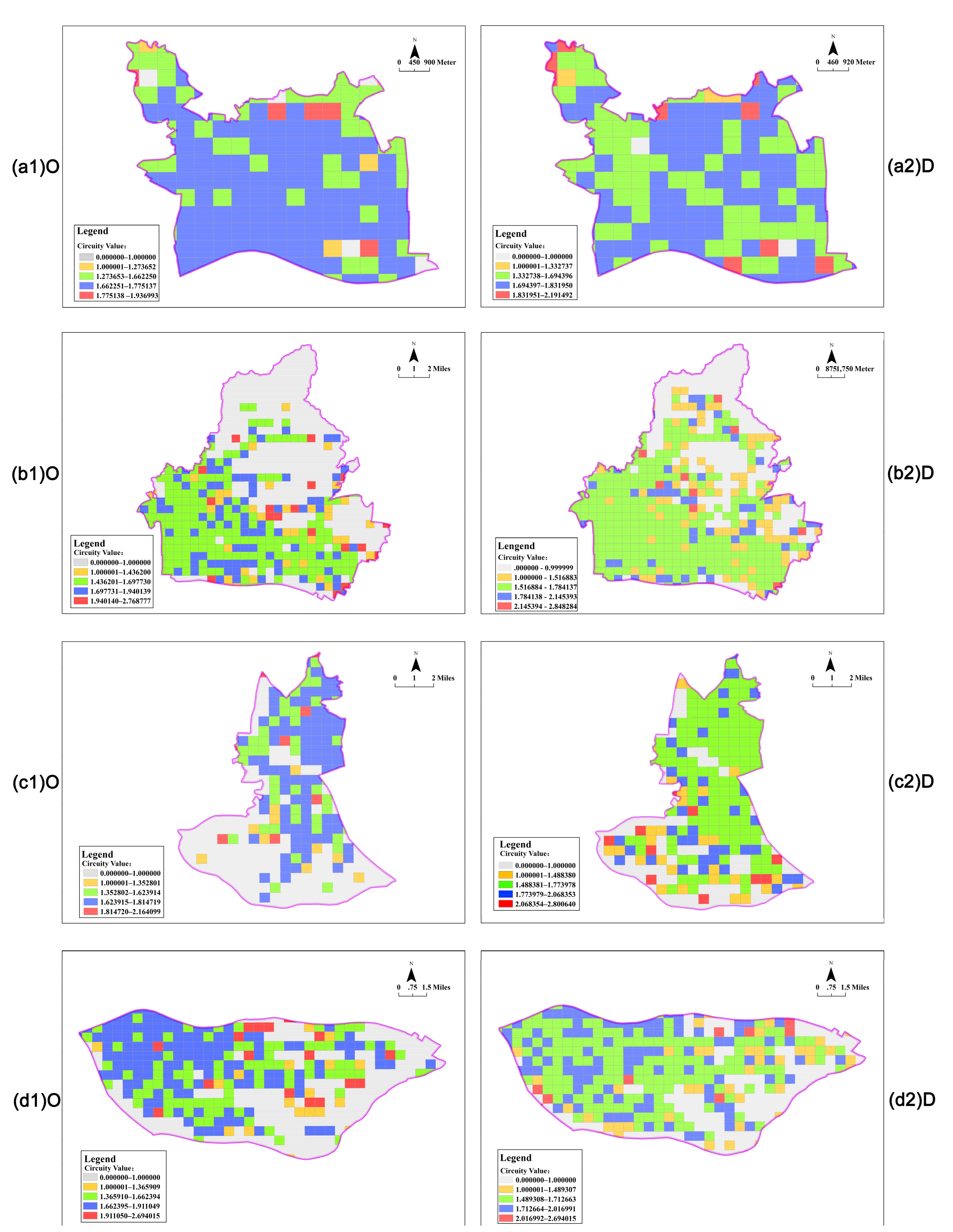
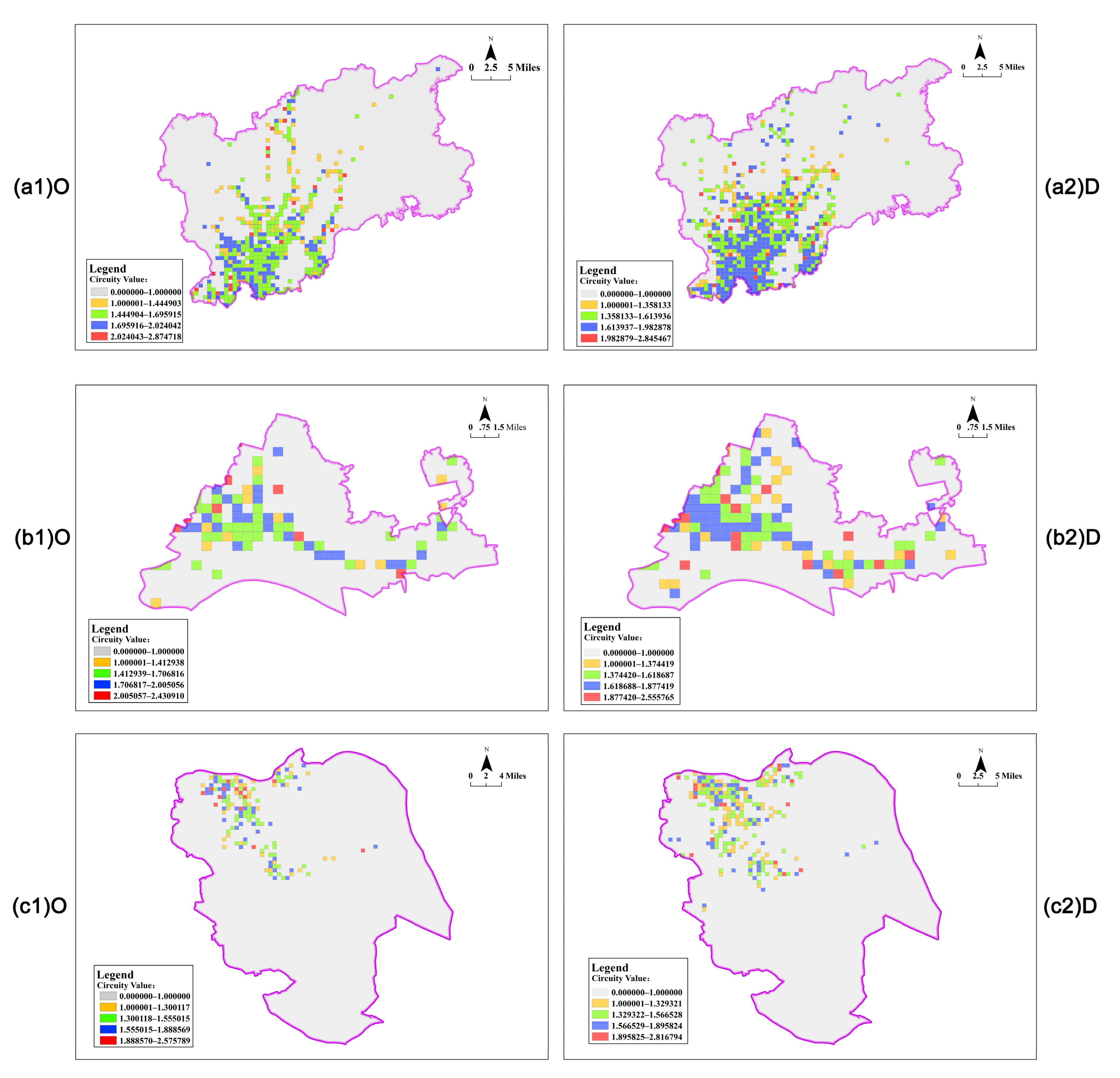
4.1.3. Travel Circuity of Each District Was Consistent, which Showed the Spatial Concentration and the Intensive Cascade Distribution
Travel circuity of each district was measured by statistics and quantitative analysis within the core area, the transition area and the fringe area. In this study, the relationships between travel circuity and distance of each district within different types of areas were compared in this study, and different characteristics of travel circuity for each district within the same types of areas were explored.
Travel circuity of O points was described concerning four districts of core area in Figure 6. The travel circuity degree of Yuexiu was higher than the other three districts. Regions of Liwan and Haizhu close to Yuexiu, had greater degree of circuity. The strength of their circuity tends to increase as Yuexiu district does, while Tianhe district is a slower developing district, thus, its degree of travel circuity is lower.
Subsequently, the spatial distribution of travel circuity for the three districts withinthe transition area is compared in Figure 7. Urban travel focuses on the region that is close to the core area of the district affected by the taxi FCD. It was found that the high travel circuity regions were also concentrated in the area close to the core area. The regions which were far away from the core area presented lower circuity. However, Baiyun district was the opposite, where it was closer to the core area it displayed, with lower travel circuity, indicating that the convergence of Baiyun district and the core area was closer.
4.2. Temporal Distribution of Travel Circuity
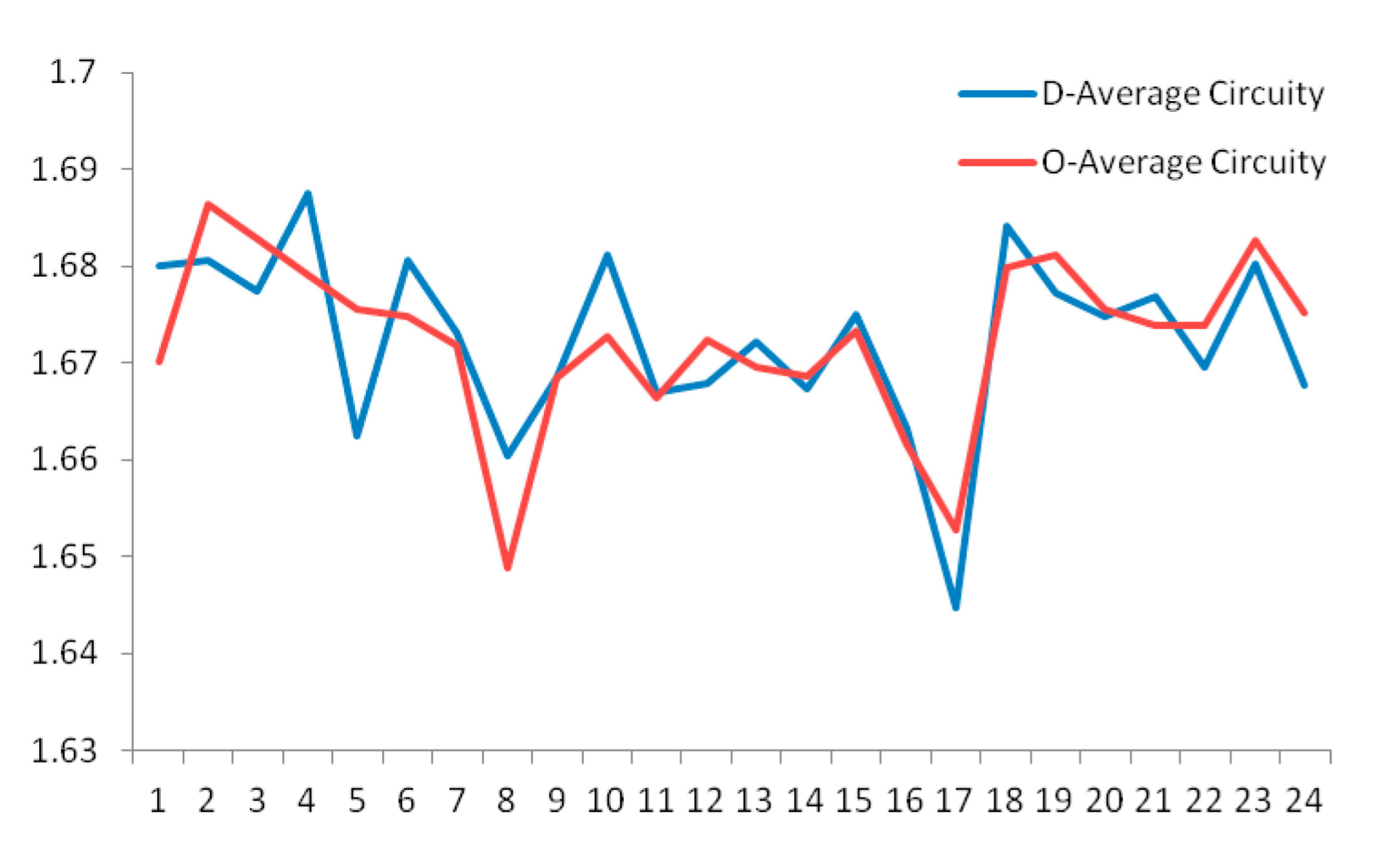
4.2.1. Peaks and Troughs of Travel Circuity Appear
Depending on the observation on the change of average travel circuity in 24 h, it was found that the value of travel circuity increased rapidly from 7:00 a.m. to 10:00 a.m. and 6:00 p.m. to 7:00 p.m. The average travel circuity values of O points rose faster in the morning, from 1.64 to 1.66 in two hours. The average travel circuity values of D points were alternately larger in the afternoon, which is increased from 1.64 to1.68 in two hours. Figure 8 presents the temporal distribution of travel circuity in 24 h.
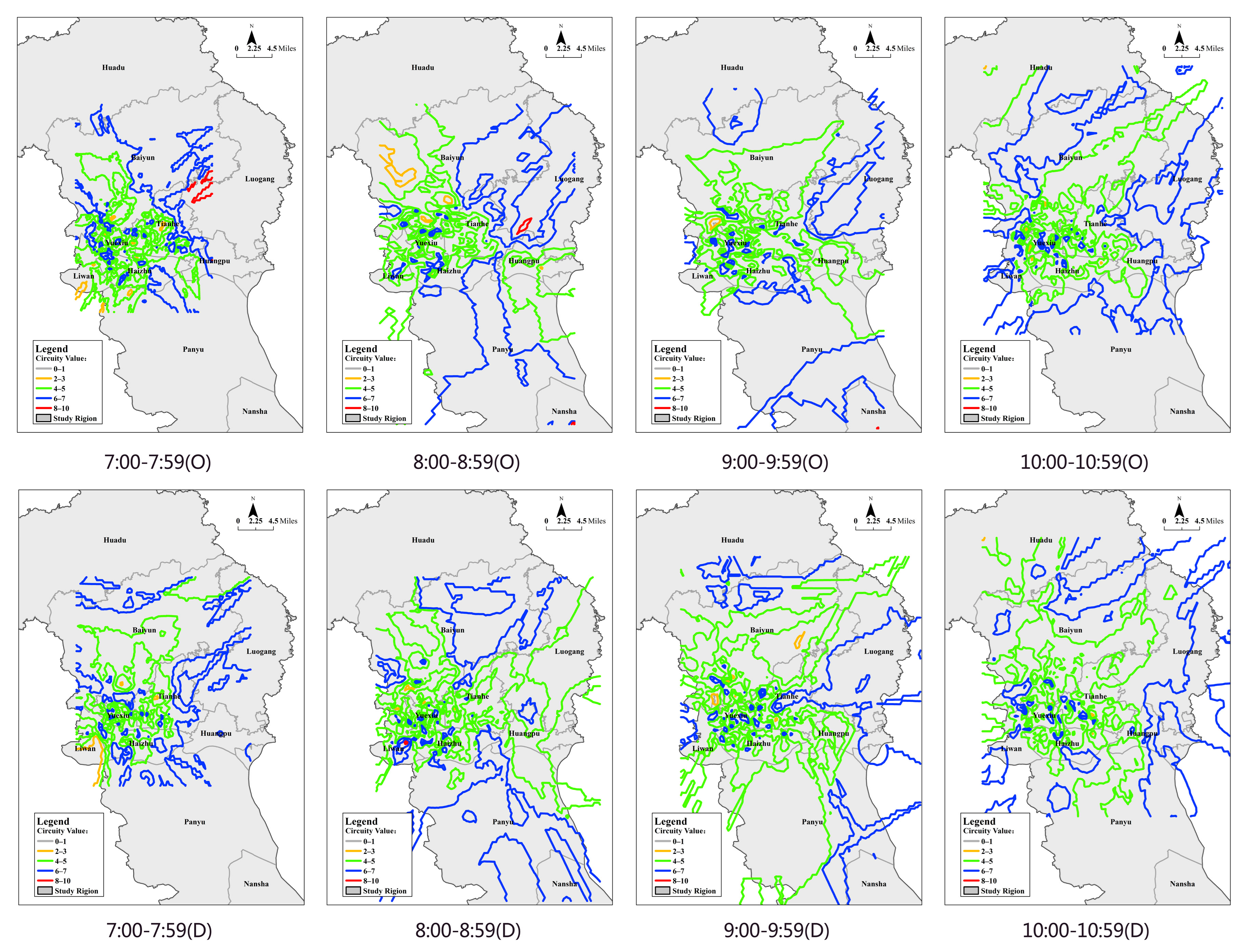
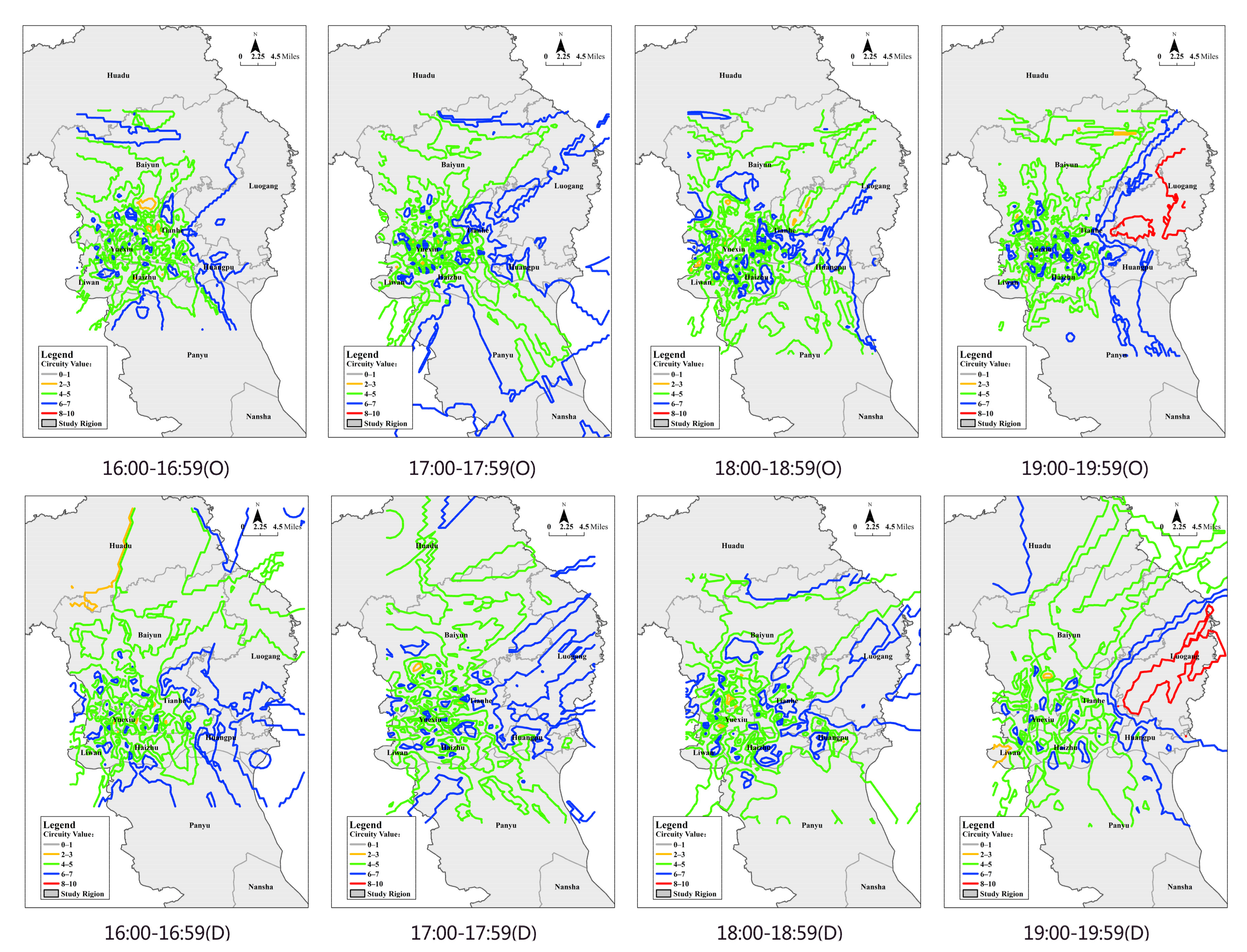
4.2.2. Travel Circuity Shows the Regional Transfer in the Morning and Evening Peak Hours
Defining the is oline of travel circuity in various period was found that travel circuity of O and D points converged on the transfer area in the morning and evening peak hours, when a ribbon gallery distribution appeared. During the time from 7:00 a.m. to 9:00 a.m., travel circuity transfer from Baiyun, Panyu and Luogang to Yuexiu, Haizhu and Tianhe, and spread from the fringe area to core area. The range from 9:00 a.m. to 10:00 a.m. showed the travel circuity of the core and fringe area was greater than the transition area. During other periods, the distribution of travel circuity was more balanced. Beginning at 5:00 p.m. to 7:00 p.m., travel circuity was appropriate to provide the delivery from the core area to the fringe area. Finishing at the end of evening peak hours, it demonstrated a large area of travel circuity in Luogang, a fringe area. Figure 9 shows the distribution of travel circuity in different periods.
5. Regression Analysis Results
5.1. The Relationship between Travel Circuity and Time
5.1.1. Results of Linear Regression Analysis
By using linear regression analysis to find out the relationship between travel circuity and time, the value of p-value (p) is 0.001. The relationship between travel circuity and time is significant. The value of coefficient of correlation (R) is –0.864, it can be found that the longer travel time is, the smaller travel circuity is. The value of coefficient of determination (R2) is closer adjusted R2, which means the linear regression model is higher reliable. The standard deviation is 3.45 which shows that the observed value and fitted curves are close.Table 1 showsthe result of regression analysis between travel circuity and travel time.
5.1.2. The Shorter Travel Time, the Higher Travel Circuity
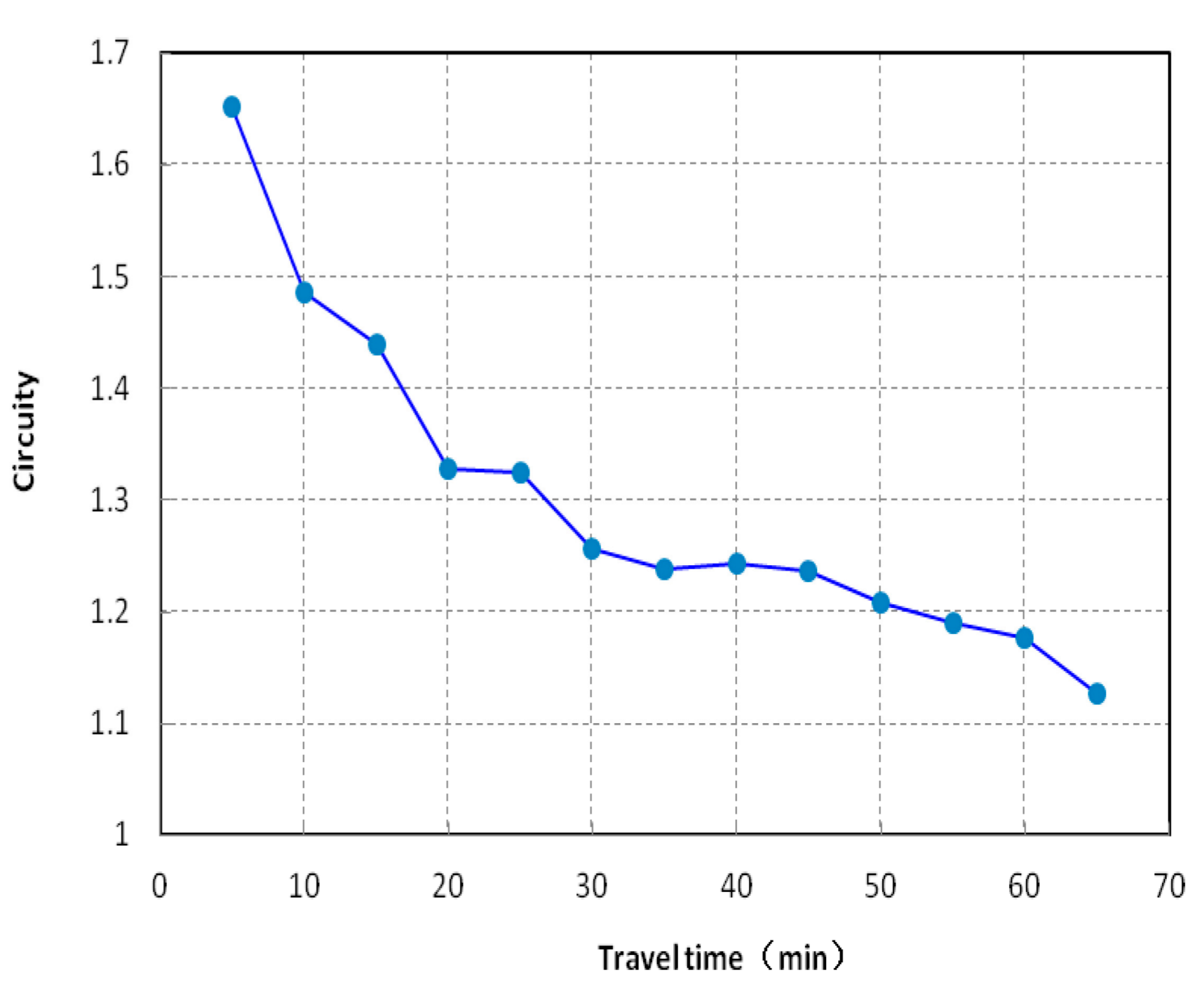
Figure 10 presents the linear relationship of travel time and travel circuity. Travel circuity decreased with the increase of travel time. The value of travel circuity declined fast in 5–10 min of travel time. The probability and degree of travel circuity for a five minutes travel time were higher than for that of 10 min, which might be formed under the influence of the density road networks.
5.2.Relationship between Travel Circuity and Distance
5.2.1. Results of Linear Regression Analysis
Using linear regression analysis to find out the relationship between travel circuity and distance, the value of p was 0.003. The relationship between travel circuity and distance was significant. The value of R is –0.888, and it was found that the longer travel distance was, the smaller travel circuity was. The value of R2 was closer adjusted R2, which means the linear regression model was higher reliable. The standard deviation was 3.91 which showed that the observed value and fitted curves are close. Table 2 exhibits the result of regression analysis on travel circuity and travel distance.
5.2.2. Circuity Decreases with the Increase in Travel Distance
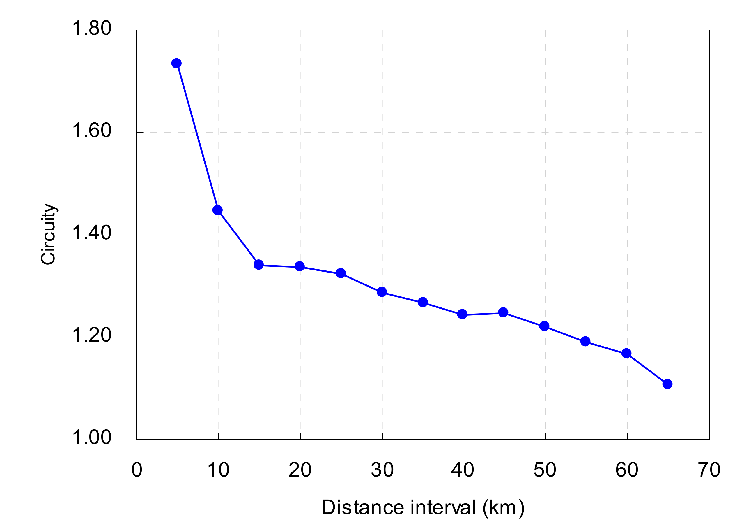
Through statistical analysis of the Guangzhou travel circuity in Figure 11, the relationship between travel circuity and travel distance was found, that is, travel circuity decreased with the increase of the travel distance. It can be noted that the circuity of the travel distance within 5–10 km declined with the fastest speed, which means that the 5 km of travel distance had a higher probability and stronger circuity than the 10 km travel distance. Thus, it was influenced by the characteristics of the road network structure and travel habits.
5.2.3. The Lower Travel Circuity, the Longer Travel Distance in the Core Areas
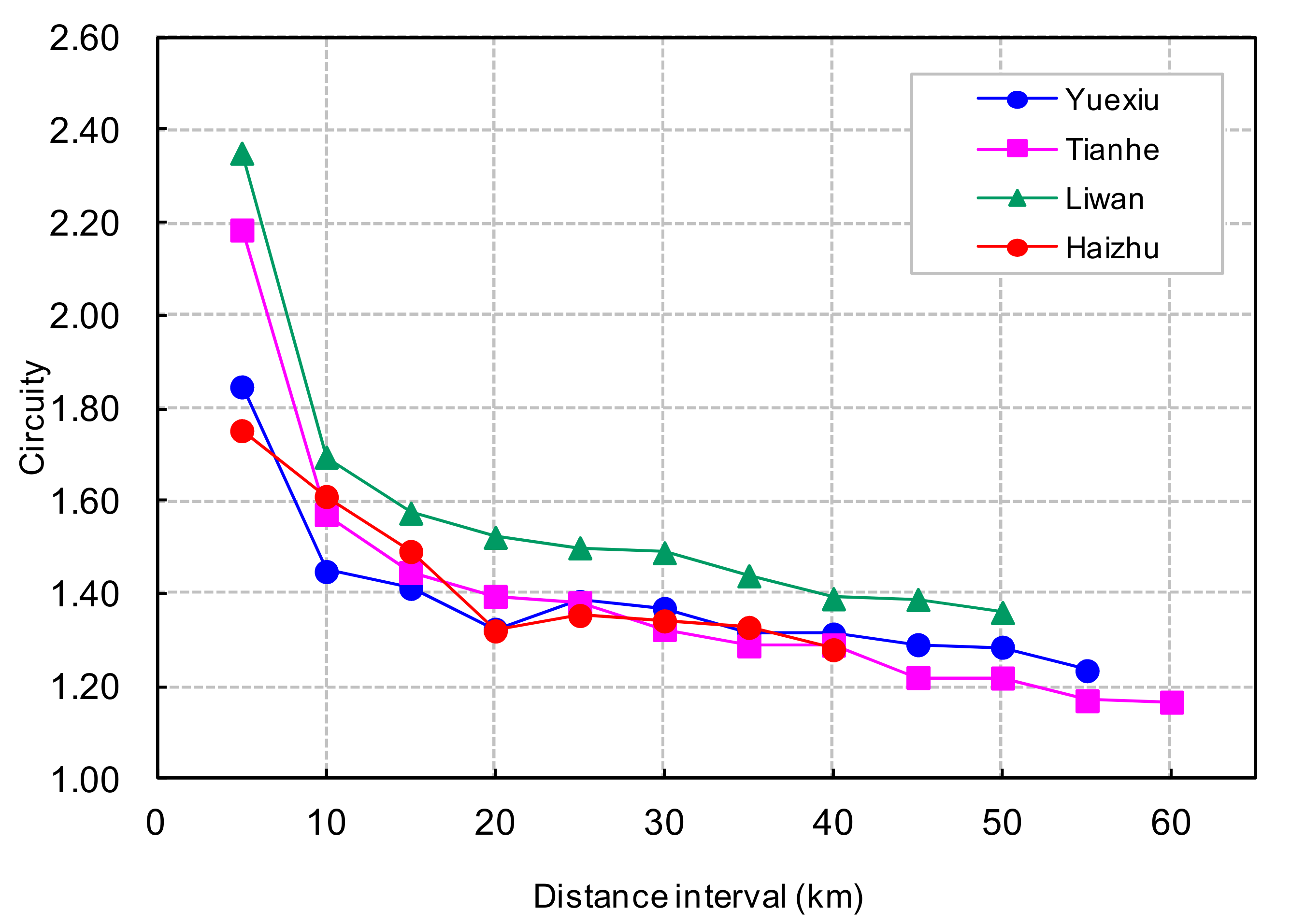
The travel distance in the range of 5 km showed a higher travel circuity at the four districts of the core area. The circuity tended to be a rapid downward trend, that is, the shorter the travel distance, the higher travel circuity.
Comparing the relationship between travel circuity and travel distance in four urban districts, it was found that the degree of circuity for Liwan was higher than the other three districts, that are far away from the fringe area. Yuexiu was slightly lower than the other three districts close to the fringe area. Figure 12 shows the relationship between circuity and travel distance in urban core area.
5.2.4. Travel Circuity Districts Increasing with the Growth of the Travel Distance when Travelling from the Transition Area to the Other Area
The travel distance in the range of 5 km showed a higher travel circuity in the transition area, while it was slightly lower than the districts in the core area. The circuity with the travel distance in the range of 5–10 km also displayed a rapid downward trend, which means when the city core area of the trip was internal travel, travel circuity was higher.
Observing the relationship between travel circuity and travel distance in three urban districts, it was found that the travel distance in the range of 10–30 km in Baiyun district showed an increasing trend. The travel circuity of Baiyun district increased with the growth of the travel distance when travelling to outside districts. Namely, there might be a bottleneck in the road network. Figure 13 presents the relationship between travel circuity and distance in the transition area.
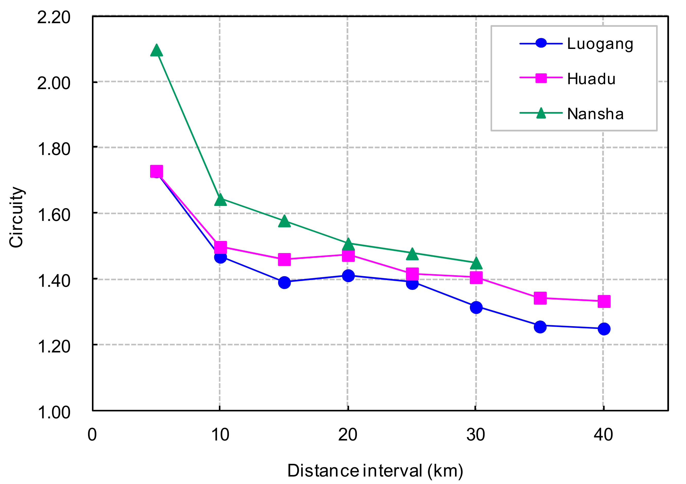
5.2.5. Travel Circuity Is Higher When the Fringe Regionis Far Away from the Core Area
When focusing on the three urban areas of the fringe region, it was found that the travel distance in the range of 5 km showed high travel circuity, but its value is slightly higher than the transition area of the city. Travel circuity tended to be a rapidly declining trend when the trip distance was in the range of 5–10 km. Comparing the relation between travel circuity and travel distance in three area of the fringe region, the travel circuity degree of Nansha was higher than that of the other two districts. The travel circuity degree was affected by the district location and transport network structure of Nansha. There was long distance between the Nansha’s surrounding area and the core area and is less developed road network. Figure 14 illustrates the relationship between travel circuity and the distance in the fringe area.
Through observing the relationship between circuity and distance/time, we found the reason of the result. When the time or distance of travel is short, travel circuity is higher. That is because when the time or distance of travel is short, the area between the city travel OD pairs is always cut piecemeal by the urban road or closed community. Then, the travel path of residents is hindered. In addition, when the time or distance of travel is long, travel circuity is lower. It can be explained by the reason that the linear distance of the travel OD pairs gets longer although, but the actual travel path between O point and D point becomes more continuous, while of which choices increase. Additionally, the travel circuity of different urban areas in mega-cities are also changed with the distinctions of urban area location and traffic network structure. In the process of urban planning and design, we should pay more attention to the layout planning of neighborhood community and the continuity of short time or short distance travel.
6. The Influence of Environmental Factors on Travel Circuity
To find the factors that influence the relationship among travel circuity, travel time and the travel distance, the factors such as urban society, structure and public transportation environment were introduced as these factors are closely associated with sustainable urban transport. They were conducive to exploring the influence factors of travel circuity. Afterwards, environmental factors that affect travel were analyzed. The influence of the environmental characteristics of O points and D points on the travel circuity was then discussed.
6.1. Environmental Factors Influencing Travel Circuity
Analyzing relevant literature shows that the urban social environment, urban form environment and public traffic environment have an obvious influence on travel time and the travel distance [29,30,31,32,33]. Due to the limitation of relevant data, this paper focused on analyzing the influence of population density, road density, the distance with city center, density of bus stations and bus line density on urban travel circuity. Table 3 shows the environmental factors influencing travel circuity.
6.2. The Influence of Environment Factors on Travel Circuity
The influence of environmental factors on travel circuity was investigated. This paper mainly analyzed the relationship of the environmental factors of O-point and D-point grid in GPS travel data and travel circuity. Through the multivariate linear regression model, the influence of six factors on cities was explored. Travel circuity was observed in three aspects, respectively, social, morphological and the public transport aspects. Table 3 shows the results of the model.
Table 4 is the regression result between the six environmental factors and travel circuity of the grid with O and D in the GPS travel data. The regression results are significant. It was found from the model results that road connectivity, the distance from the OD point to the center of the city and the station density were –0.066, –0.049, –1.063, –0.045,–0.185 and –1.011. The travel circuity of O Points and D points decreased as these three factors increased, which means that either O-point or D-Point. When the grid is closer to the center of the city, road connectivity and station density of the grid is lower and travel circuity of the grid was higher. It is worth noting that the coefficients of population density, road density and bus line density were positive. The results show that with the increase of road density, and bus line density, the travel circuity value will accordingly increase. It indicates that the increase of road and bus lines in urban planning does not necessarily contribute to improving travel circuity.
Comparing the influence of environmental factors among OD points, the effects of environmental factors on travel circuity of different OD points were obtained. It was observed from regression coefficients that when the travel circuity of O points and D points was consistent, population density and road density of the O point were higher than the D point, and the bus line density at D point was higher than that at the O point. The distance to the city center can be explained. To be specific, when the travel circuity of the O point was the same as the D point, the location of the O-point grid was further away from the city center than the location of the D point grid. It indicated that the greater the density of roads and the bus line, the closer the distance to the city center, and the travel circuity value of O points is higher than the D point. During the process of urban planning, it is not necessarily effective to increase road density or bus line density to improve travel efficiency of the O point.
7. Conclusions
Based on FCD, travel circuity can be used to describe the efficiency of a part of urban residents’ travel, which has been paid more and more attention. Taxi is an important transport mode for individual residents, and taxi customers also from an important component of urban travellers. Taxi data can reflect some residents’ travel circuity, and it is meaningful to study the travel efficiency. The taxi GPS data is used to calculate the travel circuity of individual transport in this paper. It is mainly influenced by urban population, road network structure and public transport. It can better describe the travel efficiency of individual transport. Under the restriction of the research condition, it is difficult to obtain GPS data of whole-mode and all individual trips of urban residents at present. However, with the improvement of research conditions, more types of GPS data will be available in the future. It is possible to apply them to travel-circuitous observations. Floating car data as the core component of the traffic big data, can accurately reflect the travel indirectness. Once the long-term follow-up study can be conducted, it will be a strong support for the transportation efficiency assessment.
Travel circuity characteristics are analyzed from three different scales, including the entire city, three regions and each district of city. This study obtains the spatial and temporal distribution of travel circuity, and discusses the relationship between the travel circuity and travel distance and time. It is worth nothing that the intensity of travel circuity in the same area is shown as a partial inconsistency when the area is an origin point and the destination point. It may have relationship with the number of trips and travel distance and other factors. The core area, transition area and the edge of the area is formed by the development of cities. There is the travel circuity distribution and intensity differences in different areas of the city, mainly due to the impact of transport network and the travel habits under the background of the development of urban spatial structure.
There is a strong correlation among travel circuity, the travel distance and time. It can be found that the longer the travel distance or the travel time is, the smaller travel circuity is. The relation between travel circuity and the travel distance or time also means that when travel in short time or short distance, the area between the urban travel OD is cut by the city road or closed community. Residents’ travel is hindered in this care. The travel circuity of different urban areas in mega-cities also changed with the difference in the urban location and the traffic network structure.
The influence of urban society, form and public traffic environment on travel circuity is significant. The increase of roads and bus lines in terms of road density and bus line density does not necessarily help improve travel circuity. The number of new roads or bus lines in the process of sustainable transport development might not be in favor of enhancing travel efficiency. The influences of population density, road density, the distance with city center, density of bus stations and bus line density are mainly considered in this paper, but there are some other factors that also impact travel circuity, such as employment density, the traffic volume, land use mix, road connectivity and taxi fares. Since constrained by the difficulty of obtaining data, if research conditions are ripe in future, the impact of the factors on travel circuity will be discussed in the next study.
In order to have anin-depth understanding of the residents’ travel efficiency, an important issue is how to decrease urban travel circuity. Based on some elements of sustainable cities, such as, the population, land use and the public transport, further studies should simulate the change of the urban environment, and discuss the effect of environmental factors on travel circuity reduction. Through discussing Senaratne and Goodchild about the quality of VGI [34,35], we found that in case VGI data sources are used in research studies, it is important to pay attention to the quality of such data sources before using them in the research analyses.
Acknowledgments
The authors are supported by the Foundation: National Natural Science Foundation of China, No. 41671160 and No. 41171139.
Author Contributions
Xiaoshu Cao and Feiwen Liang developed the main ideas and wrote the manuscript; Feiwen Liang, Huiling Chen and Yongwei Liu preprocessed and analyzed the data. Feiwen Liang and Huiling Chen provided helped in proofreading the article.
Conflicts of Interest
The authors declare no conflict of interest.
References
- Levinson, D.M.; Krizek, K.J. Planning for Place and Plexus: Metropolitan Land Use and Transport; Routledge: Abingdon, UK, 2007. [Google Scholar]
- Zegras, C. Sustainable transport indicators and assessment methodologies. In Proceedings of the Biannual Conference and Exhibit of the Clean Air Initiative for Latin American Cities, São Paulo, Brazil, 25–27 July 2006; pp. 25–27. [Google Scholar]
- Banister, D. The sustainable mobility paradigm. Transp. Policy. 2008, 15, 73–80. [Google Scholar] [CrossRef]
- Kennedy, C.; Miller, E.; Shalaby, A.; Maclean, H.; Coleman, J. The four pillars of sustainable urban transportation. Transp. Rev. 2005, 25, 393–414. [Google Scholar] [CrossRef]
- Weibull, J.W. An axiomatic approach to the measurement of accessibility. Reg. Sci. Urban Econ. 1976, 6, 357–379. [Google Scholar] [CrossRef]
- Levinson, D. Perspectives on efficiency in transportation. Int. J. Transp. Manag. 2003, 1, 145–155. [Google Scholar] [CrossRef]
- Boschmann, E.E.; Kwan, M.P. Toward socially sustainable urban transportation: Progress and potentials. Int. J. Sustain. Transp. 2008, 2, 138–157. [Google Scholar] [CrossRef]
- Ballou, R.H.; Rahardja, H.; Sakai, N. Selected country circuity factors for road travel distance estimation. Transp. Res. Part A 2002, 36, 843–848. [Google Scholar] [CrossRef]
- Kaplan, D.; Clapper, T. Traffic Congestion on a University Campus; Society for College and University Planning: Ann Arbor, MI, USA, 2007; pp. 28–39. [Google Scholar]
- Brimberg, J.; Love, R.F. A new distance function for modeling travel distances in a transportation network. Transp. Sci. 1992, 26, 127–137. [Google Scholar] [CrossRef]
- Boccaletti, S.; Latora, V.; Moreno, Y.; Chavez, M.; Hwang, D. U. Complex networks: Structure and dynamics. Phys. Rep. 2006, 424, 175–308. [Google Scholar] [CrossRef]
- Wolf, J.; Schoenfelder, S.; Samaga, U.; Oliveira, M.; Axhausen, K. Eightyweeks of global positioning system traces: Approaches to enriching trip information. Transp. Res. Rec. 2004, 1870, 46–54. [Google Scholar] [CrossRef]
- Cervero, R. Road expansion, urban growth, and induced travel: A path analysis. J. Am. Plan. Assoc. 2003, 69, 145–163. [Google Scholar] [CrossRef]
- Noland, R.B.; Hanson, C.S. How Does Induced Travel Affect Sustainable Transportation Policy? In Transport beyond Oil; Island Press/Center for Resource Economics: Washington, DC, USA, 2013; pp. 70–85. [Google Scholar]
- Chakraborty, A.; Allred, D. Connecting regional governance, urban form, and energy use: Opportunities and limitations. Curr. Sustain. Renew. Energy Rep. 2015, 2, 114–120. [Google Scholar] [CrossRef]
- Levinson, D.; El-Geneidy, A. The minimum circuity frontier and the journey to work. Reg. Sci. Urban Econ. 2009, 39, 732–738. [Google Scholar] [CrossRef]
- Barthélemy, M. Spatial networks. Phys. Rep. 2011, 499, 1–101. [Google Scholar] [CrossRef]
- Giacomin, D.J.; Levinson, D.M. Road network circuity in metropolitan areas. Environ. Plan. B. 2015, 42, 1040–1053. [Google Scholar] [CrossRef]
- Huang, J.; Levinson, D.M. Circuity in urban transit network. J. Transp. Geogr. 2015, 48, 145–153. [Google Scholar] [CrossRef]
- Simroth, A.; Zahle, H. Travel time prediction using floating car data applied to logistics planning. IEEE Trans. Intell. Transp. Syst. 2011, 12, 243–253. [Google Scholar] [CrossRef]
- Ben-Akiva, M.E.; Gao, S.; Wei, Z.; Wen, Y. A dynamic traffic assignment model for highly congested urban networks. Transp. Res. Part C 2012, 24, 62–82. [Google Scholar] [CrossRef]
- Hendawi, A.M.; Sturm, E.; Oliver, D.; Shekhar, S. CrowdPath: A framework for next generation routing services using volunteered geographic information. In Proceedings of the International Symposium on Spatial and Temporal Databases, Munich, Germany, 21–23 August 2013; Springer: Berlin, Germany, 2013; pp. 456–461. [Google Scholar]
- Mobasheri, A.; Sun, Y.; Loos, L.; Ali, A. L. Are crowdsourced datasets suitable for specialized routing services? Case study of openstreetmap for routing of people with limited mobility. Sustainability 2017, 9, 997. [Google Scholar]
- Graser, A.; Straub, M.; Dragaschnig, M. Is OSM good enough for vehicle routing? A study comparing street networks in Vienna. In Progress in Location-Based Services 2014; Springer: Basel, Switzerland, 2015; pp. 3–17. [Google Scholar]
- Sun, Y.; Mobasheri, A.; Hu, X.; Wang, W. Investigating impacts of environmental factors on the cycling behavior of bicycle-sharing users. Sustainability 2017, 9, 1060. [Google Scholar] [CrossRef]
- Mooney, P.; Sun, H.; Yan, L. VGI as a dynamically updating data source in location-based services in urban environments. In Proceedings of the 2nd International Workshop on Ubiquitous Crowdsouring, Beijing, China, 17–21 September 2011; pp. 13–16. [Google Scholar]
- Crooks, A.; Pfoser, D.; Jenkins, A.; Croitoru, A.; Stefanidis, A.; Smith, D.; Karagiorgoud, S.; Efentakise, A.; Lamprianidis, G. Crowdsourcing urban form and function. Int. J. Geogr. Inf. Sci. 2015, 29, 720–741. [Google Scholar] [CrossRef]
- Wang, X.; Chi, T.; Lin, H.; Shao, J.; Yao, X.; Yang, L. A research of map-matching method for massive floating car data. J. Geo-Inf. Sci. 2015, 17, 1143–1151. [Google Scholar]
- Rahmani, M.; Koutsopoulos, H.N. Path inference from sparse floating car data for urban networks. Transp. Res. Part C 2013, 30, 41–54. [Google Scholar] [CrossRef]
- Schroedl, S.; Wagstaff, K.; Rogers, S.; Langley, P.; Wilson, C. Mining GPS traces for map refinement. Data Min. Knowl. Discov. 2004, 9, 59–87. [Google Scholar] [CrossRef]
- Vande, C.P.; Schwanen, T. Re-evaluating the impact of urban form on travel patternsin Europe and North-America. Transp. Policy 2006, 13, 229–239. [Google Scholar]
- Lila, P.C.; Anjaneyulu, M. Modeling the impact of ICT on the activity and travel behaviour of urban dwellers in Indian context. Transp. Res. Procedia 2016, 17, 418–427. [Google Scholar] [CrossRef]
- Electricwala, F.; Kumar, R. Impact of para-transit travel time reliability on urban mobility: A case study. World Rev. Intermodal Transp. Res. 2017, 6, 93–109. [Google Scholar] [CrossRef]
- Senaratne, H.; Mobasheri, A.; Ali, A.L.; Capineri, C.; Haklay, M. A review of volunteered geographic information quality assessment methods. Int. J. Geogr. Inf. Sci. 2017, 31, 139–167. [Google Scholar] [CrossRef]
- Goodchild, M.F.; Li, L. Assuring the quality of volunteered geographic information. Spat. Stat. 2012, 1, 110–120. [Google Scholar] [CrossRef]
Figure 1.
Travel circuity. (a) travel circuity of Origin–Destination (OD); (b) travel circuity on the road network.
Figure 1.
Travel circuity. (a) travel circuity of Origin–Destination (OD); (b) travel circuity on the road network.

Figure 2.
Research area and spatial distribution of valid floating car data (FCD). (a) research area; (b) the spatial distribution of valid FCD.
Figure 2.
Research area and spatial distribution of valid floating car data (FCD). (a) research area; (b) the spatial distribution of valid FCD.

Figure 3.
Spatial distribution of travel circuity of urban OD pairs. (a) the spatial distribution of travel circuity of O points; (b) the spatial distribution of travel circuity of D points.
Figure 3.
Spatial distribution of travel circuity of urban OD pairs. (a) the spatial distribution of travel circuity of O points; (b) the spatial distribution of travel circuity of D points.

Figure 4.
Spatial distribution of travel circuity in the core area and the transition area. (a) thespatial distribution of travel circuity for O points; (b) the spatial distribution of travel circuity for D points.
Figure 4.
Spatial distribution of travel circuity in the core area and the transition area. (a) thespatial distribution of travel circuity for O points; (b) the spatial distribution of travel circuity for D points.

Figure 5.
The spatial distribution of travel circuity of OD pairs in the transition area and the fringe area. (a) the spatial distribution of travel circuity of O points; (b) spatial distribution of travel circuity of D points.
Figure 5.
The spatial distribution of travel circuity of OD pairs in the transition area and the fringe area. (a) the spatial distribution of travel circuity of O points; (b) spatial distribution of travel circuity of D points.

Figure 6.
The spatial distribution of travel circuity of OD pairs in the core area. (a1,a2) the spatial distribute on of travel circuity of OD pairs of Yuexiu; (b1,b2) the spatial distribution of travel circuity of OD pairs of Tianhe; (c1,c2) the spatial distribution of travel circuity of OD pairs of Liwan; (d1,d2) the spatial distribution of travel circuity of OD pairs of Haizhu.

Figure 7.
The spatial distribution of travel circuity of OD pairs in the transition area. (a1,a2) the spatial distribution of travel circuity of OD pairs of Baiyun district; (b1,b2) the spatial distribution of travel circuity of OD pairs of Whampoa district; (c1,c2) the spatial distribution of travel circuity of OD pairs of Panyu district.

Figure 8.
Average travel circuity in 24 h.

Figure 9.
Travel circuity in morning and evening peak hours.


Figure 10.
The relationship between urban travel circuity and travel time.

Figure 11.
The relationship between urban travel circuity and travel distance.

Figure 12.
The relationship between circuity and travel distance in urban core area.

Figure 13.
The relationship between travel circuity and distance in the transition area.

Figure 14.
The relationship between travel circuity and the distance in the fringe area.


Table 1.
The result of regression analysis on travel circuity and travel time.
| Index | Regression and Coefficient Test | |||||||
|---|---|---|---|---|---|---|---|---|
| R | R2 | AdjustedR2 | SD | df1 | p | F | Result | |
| Value | –0.864 | 0.726 | 0.724 | 3.45 | 1 | 0.001 | 0.001 | Signification |
Notes: SD = Standard deviation, df1 = degree of freedom, F = F test.
Table 2.
The result of regression analysis on travel circuity and travel distance.
| Index | Regression and Coefficient Test | |||||||
|---|---|---|---|---|---|---|---|---|
| R | R2 | Adjusted R2 | SD | df1 | p | F | Result | |
| Value | –0.888 | 0.789 | 0.788 | 3.91 | 1 | 0.003 | 0.001 | Signification |
Notes: SD = Standard deviation, df1 = degree of freedom, F = F test.
Table 3.
Environmental factors influencing travel circuity.
| Environment | Variables | Description |
|---|---|---|
| Urban social environment | Population density | Number of population per square metre in grid (person/m2) |
| Urban form environment | Road density | Length of road per square metre in grid (M/m2) |
| Road connectivity | Road connectivity of the center point of the grid | |
| Distances to city center | Distance from the center point of the grid to the center of the city (m) | |
| Urban public transport | Station density | Number of bus sites in the grid area |
| Line density | Number of bus lines in the grid area |
Table 4.
Environmental factors influencing travel circuity.
| Independent Variables | H | O Points | D Points | ||||
|---|---|---|---|---|---|---|---|
| Coef | t | Sig | Coef | t | Sig | ||
| Population density | +S | 0.272 | 6.978 | *** | 0.226 | 5.911 | *** |
| Road density | +S | 0.268 | 1.825 | ** | 0.232 | 1.000 | *** |
| Line density | +S | 0.191 | 5.769 | *** | 0.311 | 7.046 | ** |
| Road connectivity | –S | –0.066 | –0.429 | *** | –0.045 | –2.437 | *** |
| Distances to city center | –S | –0.049 | –2.369 | *** | –0.185 | –1.043 | *** |
| Station density | –S | –1.063 | –12.247 | *** | –1.011 | –12.295 | *** |
Notes: ** p < 0.05, *** p < 0.01.
© 2017 by the authors. Licensee MDPI, Basel, Switzerland. This article is an open access article distributed under the terms and conditions of the Creative Commons Attribution (CC BY) license (http://creativecommons.org/licenses/by/4.0/).
Share and Cite
MDPI and ACS Style
Cao, X.; Liang, F.; Chen, H.; Liu, Y. Circuity Characteristics of Urban Travel Based on GPS Data: A Case Study of Guangzhou. Sustainability 2017, 9, 2156. https://0-doi-org.brum.beds.ac.uk/10.3390/su9112156
AMA Style
Cao X, Liang F, Chen H, Liu Y. Circuity Characteristics of Urban Travel Based on GPS Data: A Case Study of Guangzhou. Sustainability. 2017; 9(11):2156. https://0-doi-org.brum.beds.ac.uk/10.3390/su9112156
Chicago/Turabian StyleCao, Xiaoshu, Feiwen Liang, Huiling Chen, and Yongwei Liu. 2017. "Circuity Characteristics of Urban Travel Based on GPS Data: A Case Study of Guangzhou" Sustainability 9, no. 11: 2156. https://0-doi-org.brum.beds.ac.uk/10.3390/su9112156
Note that from the first issue of 2016, this journal uses article numbers instead of page numbers. See further details here.