Article

Using Synergy between Water Limnology and Satellite Imagery to Identify Algal Blooms Extent in a Brazilian Amazonian Reservoir

by
Isabel Leidiany De Sousa Brandão
1,*,
Chris M. Mannaerts
1,
Wouter Verhoef
1,
Augusto César Fonseca Saraiva
2,
Rosildo S. Paiva
3 and
Elidiane V. Da Silva
3
1
Department of Water Resources, Faculty of Geo-Information Science and Earth Observation, University of Twente, NL 7500 AE Enschede, The Netherlands
2
Analytical Center Laboratory, Belém 66815-140, Brazil
3
Institute of Biological Sciences, Federal University of Pará, Belém 66075-110, Brazil
*
Author to whom correspondence should be addressed.
Sustainability 2017, 9(12), 2194; https://0-doi-org.brum.beds.ac.uk/10.3390/su9122194
Submission received: 22 September 2017 / Revised: 21 November 2017 / Accepted: 23 November 2017 / Published: 28 November 2017
(This article belongs to the Collection Eutrophication and Sustainable Management of Water)

Abstract

:
Monitoring algal blooms from space is a very challenging task, which becomes particularly difficult when dealing with cyanobacteria blooms. Cyanobacteria are strategic organisms adapted to a wide variety of environmental conditions. In high concentrations, they form scum on the water surface, which is a concern for public health due to the production of toxins, as well as being a nuisance. Knowledge of the ecological role of these organisms is, therefore, essential when trying to estimate their extent from satellite-based data. We present a multidisciplinary approach, based on both the ecological and the optical perspective. This approach is applied in a Brazilian Amazonian reservoir using spatial and temporal scales. The ACOLITE processor is employed to perform atmospheric correction. Extent of the algal bloom is mapped with outputs such as Rayleigh reflectance atmospheric corrected images. Chlorophyll-a estimation is accomplished using a blue-green edge algorithm from the Ocean Biology Processing Group (OBPG), and shows reasonable results (R2 = 0.95; RMSE = 0.40). The SAred-NIR slope algorithm identifies the extent of the algal bloom at both the spatial and temporal scale. Unfortunately, the performance of these algorithms is most likely affected by weather conditions and glint effects. Therefore, this study recommends that cyanobacteria or phytoplankton studies in this area ensure that their ecological functioning is carefully considered when attempting to map occurrence using limited satellite imagery.

1. Introduction

Eutrophication in man-made reservoirs has received considerable attention over time due to its harmful effects on the aquatic environment and on human and animal health [1,2]. The increased probability of algal blooms occurring is of major concern, especially where these blooms are due to (toxic) cyanobacteria species. Under natural conditions in aquatic ecosystems, a balance exists between cyanobacteria and other phytoplankton groups [3]. However, specific characteristics may allow cyanobacteria to become prevalent. These characteristics are determined by a range of features, including cellular physiology (gas vesicles within cells allow regulation of buoyancy) and physiological response (light and nutrient utilization, for example), cell size, cell structure, and general morphology [4]. The predominance of cyanobacteria over other species occurs under specific environmental conditions, including optimal light intensity and water temperature, nutrient availability and stability in the water column [2].
Cyanobacteria harmful algal blooms (CHABs) form an increasing problem globally in all types of water bodies due to mounting eutrophication [5,6,7,8]. Moreover, they are responsible for a variety of impacts on environmental, economic and social scales [9]. They greatly impact on zooplankton and fish populations in aquatic ecosystems [10]. The presence or absence of particular cyanobacteria species may signal the ecological status of a water body; the dominance of cyanobacteria has been particularly useful as an indicator for a high nutrient status [11]. Thus, monitoring of cyanobacteria blooms in drinking water and reservoirs with secondary uses is necessary [12]. However, estimating the occurrence of CHABs hot spots in unmeasured locations using traditional sampling methods is very difficult [12,13,14].
Satellite remote sensing techniques offer suitable tools to integrate large-scale water quality monitoring data [15,16] and have been widely used to estimate Chlorophyll-a [16,17,18,19,20] and phycocyanin [21,22,23,24,25,26,27,28,29]. Cyanobacteria blooms have been studied using the bio-optical approach based on retrieval algorithms for phycocyanin, a specific pigment of cyanobacteria. Very few methods use multispectral data, such as Landsat, to estimate cyanobacteria density from atmospherically corrected surface reflectance values, as proposed by [30,31,32]. The main challenge is still the low availability of sensors with suitable spectral bands to retrieve cyanobacteria data using field-based approaches [33].
The Operational Land Imager (OLI) sensor onboard the Landsat-8 satellite has shown potential regarding application in studies on aquatic environments [34]. OLI images were used by [35] to estimate cyanobacteria density by means of empirical models and [36] emphasized the value of OLI images based on the blue to green spectral region for assessing waters with a low to medium amount of biomass of blue-green algae.
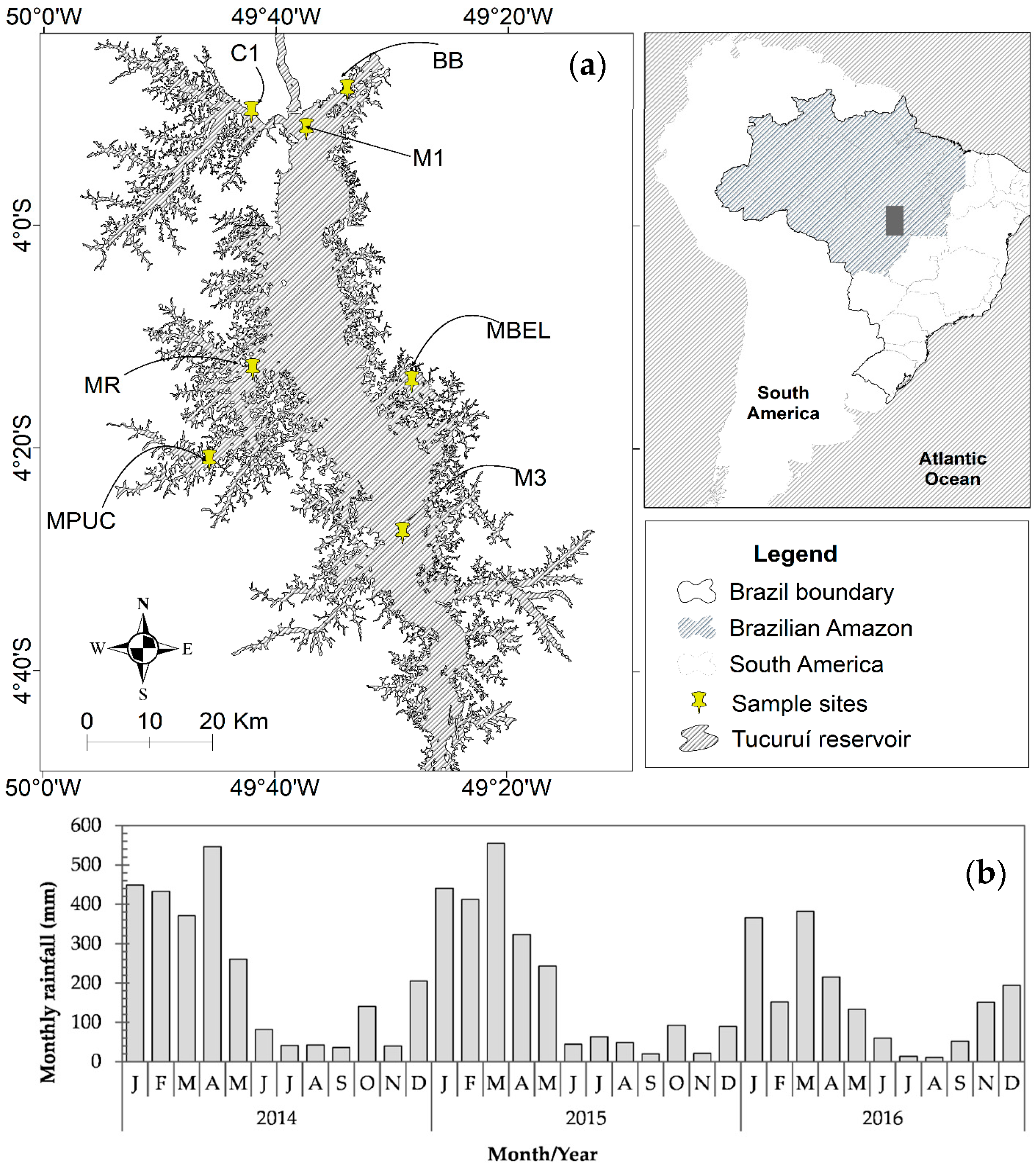
The study of CHABs in the Tucuruí hydroelectric reservoir (THR) in Brazil is of great importance, due to the multiple uses of its water by the local population. However, the reservoir has only been mentioned in a few studies [37,38] concerning phytoplankton density and never specifically regarding CHABs. Monitoring cyanobacteria density with satellite images has not been undertaken at all. Here we propose a multidisciplinary approach that aims to assess algal bloom extent and which includes ecological and optical studies, in a spatial and temporal context as supported by [39]. The first approach was based on the water limnology of the THR, consisting of physico-chemical parameters and phytoplankton studies. The latter was based on the categorization of phytoplankton according to their species’ survival strategy regarding different environmental changes. This categorization consists of a list of 31 functional phytoplankton groups, represented by alphanumeric terms, established by [40]. The use of this classification has as main objective to detect patterns in the phytoplankton dynamic and distribution, as well as relate them to environmental changes. The second approach was based on the algal bloom extent and Chlorophyll-a estimated from OLI data.
The main goal of this study was to investigate if the combination between water limnology and satellite imagery is a suitable approach to identify CHAB extent in the Tucuruí hydroelectric reservoir. This motivation was based on the characteristics of the THR water conditions (with low/medium Chlorophyll-a) and using the literature of [32,36]. The application of satellite remote sensing techniques may help to compensate for the limited spatial dimension of traditional in situ methods. It permits acquisition of necessary information at different spatial and temporal scales, allowing a more complete analysis of aquatic ecosystems, and it is a functional analysis in synoptic order. We also aim to map Chlorophyll-a on a spatial and temporal scale, as it is closely related to cyanobacteria occurrence. The outcomes of this study aim to support water management regarding CHABs impact in the Tucuruí hydroelectric reservoir.

2. Materials and Methods

2.1. Study Area

The Tucuruí hydroelectric reservoir (THR) is located in the Tocantins watershed (Amazon region) between 3°39′S 50°6′W and 4°45′S 49°23′W, Pará State, in Brazil. It is one of the largest hydroelectric reservoirs of the Amazon region with a surface area ranging between 2800 and 3000 km2 during the year and a storage capacity of 45.5 km3. The reservoir‘s length is approximately 170 km and its average width is 14 km. Study sites included 16 sampling points for Chlorophyll-a, and 7 sampling sites for phytoplankton as shown in Figure 1a,b. These sites cover different areas in the THR with their own limnological complexity.
The study area is located in a tropical region and is classified as continental. It is characterized by a wet period from January to April, and a dry period from May to December, with very low rainfall in August and September [41] (Figure 1b).
The THR has a complex dentritic pattern with a monomictic system. It is characterized by short periods of circulation, as well as thermal and chemical stratification. According to [42], it is a mesotrophic water body. The THR also shows characteristics of a reservoir in the process of stabilization with a steady decrease in phytoplankton diversity [37]. The THR has inundated a vast area of tropical rainforest, most of which was not removed during the filling phase. As described by [41], the THR has its own limnological features due to its morphometry, climatological and hydrological patterns, and relatively low retention time (45 days).
The damming of some tributaries did produce areas (such as C1 and MPUC in Figure 1a) with a high retention time. A special dynamic process occurs in these areas, leading to high stratification periods and high conductivity in lowermost water [43]. Due to reduction in water velocity and nutrient accumulation, the biomass and the diversity of biological life is higher in these areas [44].
The main purpose of this reservoir was electricity generation; however, secondary uses have been noticed such as fish-farming and recreation [45]. Although these secondary uses require lower water quality standards than necessary for drinking water, the Brazilian legislation (CONAMA) has established certain criteria for secondary uses. These include maximum values for Chl-a (10 mg m−3), cyanobacteria density (20.000 cells mL−1) or biovolume (2 mm3 L−1), turbidity (100 NTU), and color (75 mg Pt Co L−1).

2.2. Field Survey Methodology

Two field surveys were conducted at two different water level phases of the THR, which is full from February to May, and emptying from July to August. The first field survey was conducted in April, and the second in July of 2016. The field survey times were chosen in order to show the cyanobacteria spatial and temporal variability between full and dry reservoir phases and to coincide, where possible, with Landsat 8 satellite overpasses during cloud-free periods. As the Amazon region is covered in cloud most months, it was difficult to study periods of high rainfall (Figure 1b).

2.2.1. Phytoplankton Sampling and Analysis

Samples displaying physico-chemical and biological parameters were collected at 7 sites during the four fieldwork campaigns and analyzed using standard methods described in [46]. The following variables were measured: dissolved oxygen (SM 4500-OC); temperature (digital thermometer, SM 2550); pH (PHTEK device, NBR 9896/1993); suspended solids ( SM 2540-D; transparency (Secchi disk); nitrite (SM 4500-NO2-B); nitrate (SM 4500-NO3-B); ion ammonium (SM 4500NH3C); phosphate (SM4500-PC), and Chlorophyll-a (extraction by acetone [47]). Phytoplankton was sampled in the morning using plankton netting of 20 µm, fixed in the water at a depth of one meter with the boat moving at low-speed for about three minutes at each sampling site. These samples were collected in 250 mL bottles and used for qualitative analysis. For quantitative analysis, samples were collected from the water surface with 500 mL bottles. Samples were fixed with 4% Lugol’s solution at a proportion of 0.5 mL to each 100 mL.
The density of phytoplankton (cell L−1) was determined by the sedimentation method and analyzed under an inverted microscope (Zeiss135) using a maximum magnification of 400× as described in [48] and different chamber sizes ranging from 2 mL to 6 mL. Qualitative analyses were performed using non-permanent slides with 1 mL subsamples. Approximately 10 to 15 counts were conducted per slide until the first 100 individuals of the same species were observed. This analysis was realized using a binocular microscope with 40× and 100× lenses (Leica). The species were identified to the lowest possible taxonomic level, based on [49]. Phytoplankton biomass and biovolume were estimated based on the cell or colony linear dimensions according to [50] using the same inverted microscope as we used to measure phytoplankton density, and expressed in [mg (fresh weight m−3)], where 1 mm3 = 1 mg m−3, and in percentage (%) as described in [51].
Descriptive statistics and correlation tests were performed to evaluate the dataset obtained in this survey. Descriptive statistics were accomplished through determination of the minimum, maximum and average values as well as standard deviation and coefficient of variation. Analysis of variance was performed through a Kruskal-Wallis test to investigate differences between spatial and temporal scales of limnology parameters with p < 0.05 significance. Correlation tests were assessed through the Pearson coefficient with p < 0.05. Statistical analyses were performed using the program RStudio version 1.0.153 (RStudio, Boston, MA, USA) [52].

2.2.2. Water Sampling and Analysis

The limnological measurements were made available by the Centre of Environmental Protection of Eletrobras-Eletronorte (the company responsible for monitoring the water quality in the THR). Water samples were measured every two months (from 2014 to 2016) at 16 locations and filtered through a Whatman GF/52-C glass fiber filter, 47 mm in diameter and with a 1.2 µm pore size, to estimate the Chl-a concentration in the laboratory. The filter was frozen and kept in the dark until further analysis was undertaken. The Chl-a concentration was estimated using the extraction-by-acetone method through spectrophotometric analysis and a time-series is shown in the Supplementary Materials Figure S2.

2.2.3. Remote Sensing Data Processing

In this study, we tested five scenes (on path 224, row 63) acquired between June 2013 and September 2016 by the OLI multispectral sensor onboard of Landsat 8. Of the selected scenes, only the data of those presenting clear skies and cloud-free conditions over the Chlorophyll-a sample sites were considered. The free availability of data from the United States Geological Survey (USGS) (http://earthexplorer.usgs.gov/), as well as the temporal resolution of 16 days of the OLI sensor, provide certain advantages over other sensors. Orthorectified and terrain corrected Level1 OLI imagery was obtained. Imagery of the USGS website is processed by the Level 1 Product generation System (LPGS) and is provided in GeoTIFF format with UTM projection and WGS84 datum. The fieldwork data were collected approximately three days before and/or after the overpass of the OLI sensor for all scenes. The main characteristics of the OLI sensor are summarized in Table 1.
According to [53], the atmospheric correction of satellite measurements in aquatic ecosystems is very important for the reason that a large part of radiation detected by the sensor is backscatter from the atmosphere. Thus, to properly identify the pixel content in an image in terms of water quality, the atmospheric correction presents a critical step in data processing of satellite images [54].
The atmospheric correction was performed using the ACOLITE—a binary processor for atmospheric correction developed by the Royal Belgium Institute of Natural Science (RBINS), which uses the Gordon and Wang approach [55]. The ACOLITE allows for a robust and easy atmospheric correction. This process is fully described in [56,57]. Basically, the processor performs an atmospheric correction in two steps: (1) a Rayleigh correction for scattering by air molecules, using a Look-Up Table generated using 6SV [58]; and (2) an aerosol correction based on the short wavelength infrared (SWIR) band. Output of ACOLITE is the water-leaving radiance reflectance (referred as ρ w), remote sensing reflectance (Rrs), among others, which can be used to compute multiple other parameters, such as Chl-a and turbidity [59]. A summary of the atmospheric correction flow used in this study is shown in the Figure A1 in Appendix A.
Moreover, this processor allows for the creation of an image subset to separate water (the area of interest) from land and cloud. To apply image processing procedures on the water covered areas, an image masking procedure was thus applied. In the masking process, the SWIR 1 band (1609 nm) was used with a 2.15% threshold.

2.2.4. Chlorophyll-a Algorithm

The ACOLITE processor allows for a specification of outputs per wavelength. In this study, we specified outputs such as remote sensing reflectance (Rrs (sr−1)), Chlorophyll-a using an algorithm developed by the Ocean Biology Processing Group (OBPG) (http://oceancolor.gsfc.nasa.gov/), and the atmospheric correction applied here is fully described in [56] and a summary is described in Appendix A.1. The OLI sensor has appropriate bands to retrieve Chl-a concentrations using the blue-green ratio (Equation (1)) according to [59].
Chl-a (mg m−3) = 10^(a0 + a1 × R + a2 × R2 + a3 × R3 + a4 × R4),
where, R is the logarithm of the ratio of maximum blue to green reflectance, and a0 to a4 are 0.2412, −2.0546, 1.1776, −0.5538 and −0.4570, respectively. This algorithm has been calibrated for the OLI sensor by [60] in the three band configuration (~440, ~490, and ~560 nm).
A group of 21 sample matches-up and five scenes were used to assess the Chlorophyll-a concentration. All sampling matches were buffered to create a 3 × 3 pixel window corresponding to the spatial scale (pixel size) of the OLI sensor as described in [35]. The median value for the 3 × 3 window was extracted from all scenes generated by the Chl-a algorithm. After extraction of each sampling point, we proceeded with the statistical analysis to compare the measured in situ Chl-a with the values estimated by the Chl-a algorithm. Pixel extraction and map layouts were performed using the latest version of SeaDAS (version 7.4, NASA, Washington, DC, USA) available on https://seadas.gsfc.nasa.gov/ and ArcMap (version 10.5.1, ESRI, Redlands, CA, USA), respectively.

2.2.5. Algal Blooms Extent

To assess the extent of algal blooms in the THR, we used a simple slope algorithm approach (referred as SAred-NIR) developed by [32] for inland waters, using OLI and TM sensors of the Landsat imagery and Equation (2):
SA red NIR = ( ρ c ( red ) ρ c ( NIR ) λ red λ NIR ) × 1000
where, red stands for 665 nm, NIR for 865 nm and ρ c for Rayleigh corrected reflectance. A summary of the processing steps to obtain ρ c is described in Appendix A.2. This algorithm allows the identification of different classes of algal bloom, including severe and moderate bloom, which are summarized in Table 2. High probability of severe bloom of cyanobacteria occurs when SAred-NIR results are greater than the factor of 0.15 and when Chl-a concentration is higher than 50 (µg L−1). Moderated bloom is probable to occur when the results of the SAred-NIR is in the range of −0.05 to 0.15 and Chl-a 5 to 10 (µg L−1). Additionally, severe bloom is characterized by positive slope between band 4 (665 nm) and 5 (865 nm), and it is more neutral for moderated bloom and negative for non-bloom conditions according to [32].
The advantages of the SAred-NIR algorithm are its ability to identify algal blooms in the presence of thin cloud (a frequent issue in inland waters, mainly in the Amazon region) and it uses the OLI sensor products, which are freely available from the United States Geological Survey [61]. Moreover, input to the SAred-NIR algorithm in this study is level 1 data, first corrected by removing the molecular scattering effects and converted to Rayleigh corrected reflectance as described by [56,62] and summarized in Appendix A.2.

2.3. Performance Assessment

Results of the Chlorophyll-a algorithm performance was assessed using error metrics such as Mean Square Error (MSE), Mean Absolute Error (MAE), Mean Absolute Percentage Error (MAPE), Root Square error (RMSE), bias, mean normalized bias (MNB), and determination coefficient (R2), which are described in Table 3.

3. Results

3.1. Ecological, Spatial and Temporal Approaches

The ecological data, both spatial and temporal, are summarized in Table 4, which presents the main environmental characteristics of the sampling sites. Each site was characterized based on work by [43] and according to the phytoplankton functional group classification described in [40].
Our results on Table 4 showed that at the sites MPUC, MBEL, and M1 the seasonal progression passes through a sequence leading from eutrophic to mesotrophic waters. M3, however, depicts an oligotrophic to mesotrophic classification at a temporal scale. These sites are characterized by species of the M and P associations in April and the B, NA, and F associations in July.
Phytoplankton organisms of the M and P associations are typical of the turbid waters, with mixed layers, and major representatives are cyanobacteria species. Those of the B, NA, and F associations mostly represented by Chlorophyta and Zygnematophyta, are organisms thriving in clear, deeply mixed oligo to mesotrophic and meso to eutrophic waters. The sites that are situated at the dendritic regions of the reservoir (C1 and BB) (Figure 1a) are characterized in April by species adapted to eutrophic waters with low nitrogen content, and in July by species adapted to nutrient-rich, warm and mixed water columns.
Figure 2a,b presents the algae groups contribution to the total biovolume in percentage for April and July of 2016, respectively. Our results show dominance of cyanobacteria in April, while in July there is an increase of green algae and diatoms. In April, the average cyanobacteria dominance is 63.10% (±9.18) with maximum contribution of the Microcystis aeruginosa specie (27.71%) to total biovolume, while in July, cyanobacteria average is 21.95% (±6.73) with maximum contribution of the Raphidiopsis curvata specie (30.16%).
The average Chl-a concentration was 5.90 (±2.22) mg m−3 in April, and 2.85 (±1.07) mg m−3 in July (Table 5) with significant variation only in temporal scale (p < 0.01). Cyanobacteria density decreased from April to July at all sites with significant variation in temporal scale (p < 0.01) and was negatively correlated with Chl-a in April (−0.81; p < 0.05) and in July (−0.83; p < 0.05). The decreasing in cyanobacteria density and reduction of the water pH, may have favored conditions to other phytoplankton species to prevail in July. The water pH showed significant variation in temporal scale (p < 0.01). In April, Chl-a was correlated with dissolved oxygen (0.93; p < 0.02), transparency (0.98; p < 0.01), and nutrients, such as nitrate (0.98; p < 0.01), ion ammonium (0.99; p < 0.01) and phosphate (0.99; p < 0.01). In July, Chl-a was correlated with phosphate (0.87; p < 0.05), ion ammonium (0.99; p < 0.01), and nitrate (0.99; p < 0.01).
Table 5 contains descriptive statistics of the water quality parameter results. Higher values of dissolved oxygen were measured in April with an average of 5.55 (±0.69) mg L−1. Nutrients such as nitrite, nitrate, and phosphate were more abundant in July than in April with averages of 0.49 (±0.24) µg L−1, 0.22 (±0.09) mg L−1, and 11.08 (±2.96) µg L−1, respectively. The mineral silicate presented maximum concentrations in July with an average of 7.58 (±0.30) mg L−1 and significant variation in temporal scale (p < 0.01). Water transparency, which is the combination of effects of color, turbidity and algae, increased from April to July, however this parameter did not present significant spatial and temporal variation. The average color in the time series analysis (Figure S5 in the Supplementary Materials) was 29.82 (±27.76) Pt Co and this parameter varied significantly in spatial and temporal scales (p < 0.05).

3.2. Optical, Spatial and Temporal Approaches

Figure 3 shows the spectral Rayleigh corrected reflectance values at sampling sites with less weather interference (i.e., a cloudless sky and the absence of haze) acquired from the OLI sensor in (Figure 3a) April and (Figure 3b) July, 2016. This figure indicates that the spectral reflectance characteristics, which are associated with the algal bloom intensity, of the sample sites are similar in April, differing only in magnitude. The slope between band 4 (665 nm) and 5 (865 nm) is positive for severe bloom conditions due to the high absorption of Chl-a in the red region of the spectrum and high scattering of algal cells in the NIR region. The MR and M1 sites showed higher cyanobacteria relative percentage than the M3 site (see Figure 2a). On the other hand, in July the slope at the NIR region is less evident than in April, indicating high absorption of water, low scattering in the NIR region, corroborating with low Chl-a concentrations in these sites.
In addition, Figure 3 shows that sites can be distinguished according to the difference in Chl-a concentration in the visible spectral region. The MR and M1 sites will very likely see an increase in Chl-a concentration in April (Figure S2 in the Supplementary Materials), contributing to the increase in magnitude of their spectral features. Features associated with phycocyanin absorption (near 630 nm) and reflectance by Chl-a (near 720) do not occur. However, the high reflectance in the green region and low absorption in the blue region are associated with Chl-a presence [63].
Figure 4 shows the results of the SAred-NIR algorithm applied to the Rayleigh corrected reflectances in April 2016 in the false color composition (R = 665 nm, G = 561 nm, B = 483 nm). Three sites indicated the presence of algal bloom corroborating with our results in Figure 2a,b. These three sites are very likely to display severe algal blooms in April, decreasing to moderate or no bloom in July. In addition, our Chl-a results show higher concentrations in April than in July. This would classify this reservoir to eutrophic conditions while in the emptying phase, it is categorized as oligotrophic to mesotrophic due to its low Chlorophyll-a concentration.
Figure 5 shows the results of the SAred-NIR algorithm applied to the Rayleigh corrected reflectances of July, 2016. In this month, the THR is very likely to exhibit low Chl-a concentrations and oligo to mesotrophic waters. However, M3 site showed an indication of a moderate bloom and SAred-NIR varying from –0.06 to 0.05.
Figure 6 shows a plot of measured and estimated values of Chl-a. Chlorophyll-a is estimated using the OBPG algorithm and it is an output of the ACOLITE processor.
Figure 7 shows the map of Chl-a concentrations estimated by the OBPG algorithm using the coastal aerosol (443 nm), blue (483 nm) and green (561 nm) bands and the dataset of Chl-a time series. Many pixels with cloud cover and aerosol effects were not retrieved through remote sensing reflectance, resulting in such areas emerging without pixel value (i.e., white in color). For the depicted results from 2016 (spatial and temporal variation), we only used sites unaffected by weather conditions to assess the goodness of the fit between measured and estimated values (Figure 6).
Performance assessment revealed good agreement between measured and estimated Chl-a as described in Table 6.

4. Discussion

Water quality monitoring in reservoirs is an important approach to understanding the complexity of this environment. These environments are classified as ecosystems with permanent disturbance on a vertical and horizontal scale [64] and their water quality is greatly influenced by human interference.
In the case of the THR, little human interference affects its water quality, due to minimal occupation near its edges and insignificant changes in land use and cover, as is described by [65]. When the THR is full, the main source of nutrient loading is rainfall, while in the emptying phase it is the water level, which releases nutrients from the bottom [66]. The THR is characterized by areas with different limnological patterns as a result of its morphometry, and areas which were not deforested prior to the flooding [43,67].
This study proposes a multidisciplinary approach to assess the feasibility for the OLI sensor to monitor algal blooms in the THR. To this effect, an ecological and optical approach in both spatial and temporal scale is applied. An understanding of the ecological characteristics of reservoirs, including bio-physical and chemical features, is important for their water management. Biological studies are important to assess uses of water in reservoirs due to their close relation to the effects of algal blooms. Enhanced phytoplankton growth is a major concern for policy and management particularly when the reservoir is used for recreation, aquaculture or potable supplies [68].
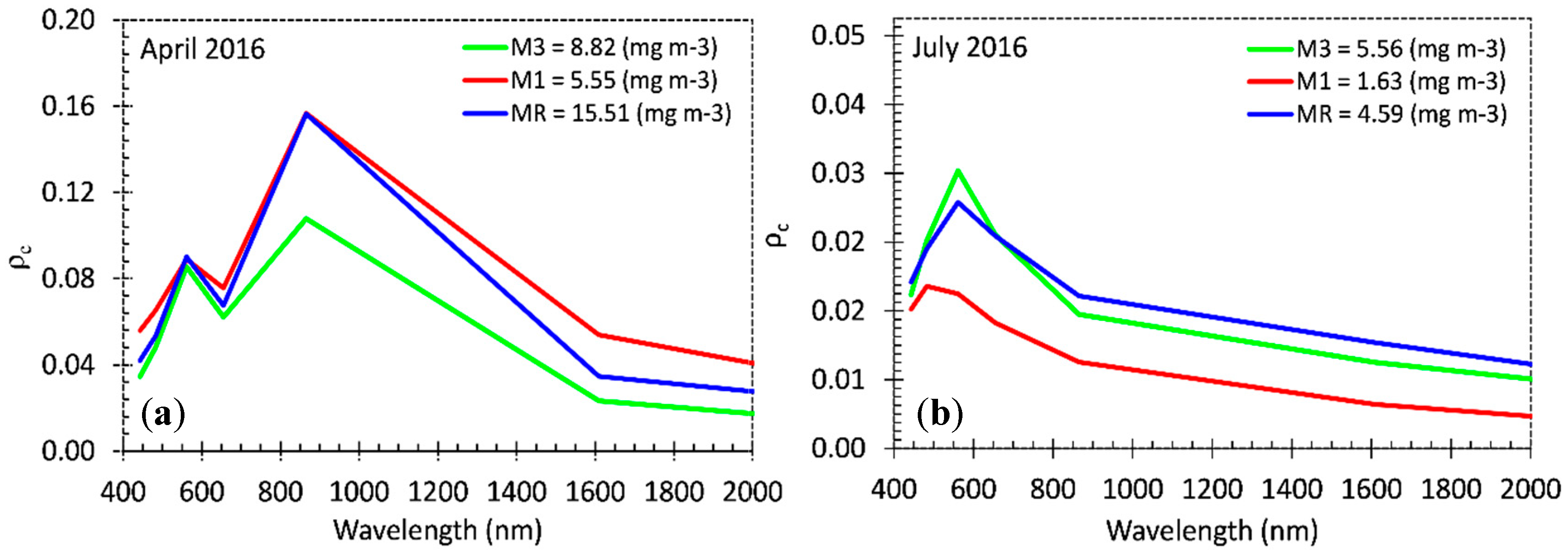
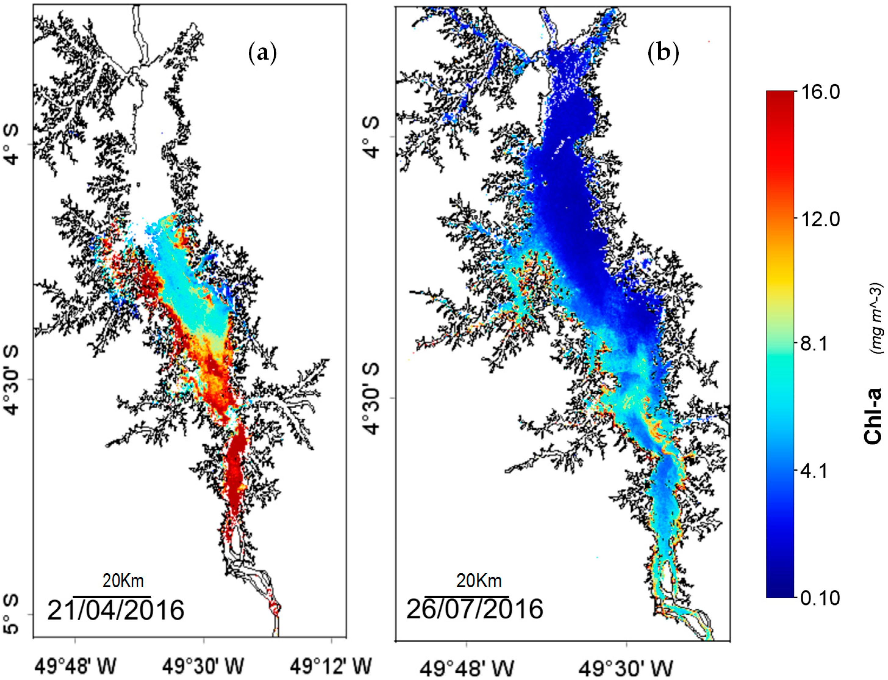
Our results show that Chl-a concentrations were higher in April (full reservoir and at the river zone) at 15.51 mg m−3 than in July at 4.10 mg m−3. Significant variation (p < 0.05) of Chl-a concentration was found between months but not in spatial scale. In the full phase of the reservoir, Chl-a tends to increase at certain sites near dendritic and edge areas. In April, Chl-a concentrations in the water were in the range of eutrophic, while in July the range reached oligotrophic to mesotrophic values. Da Costa Lobato et al. [42] showed similar results in the emptying phase of the reservoir (June to August), classifying this reservoir as mesotrophic with few oligotrophic sites. Low trophic levels in this reservoir could be related to its stabilization process, which is a positive factor for the maintenance of the phytoplankton diversity and biomass [2].
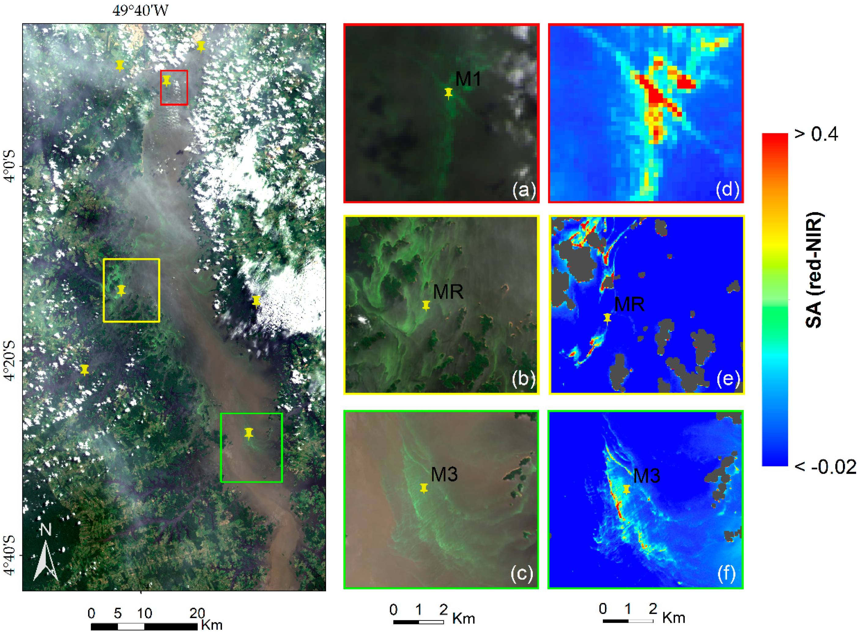
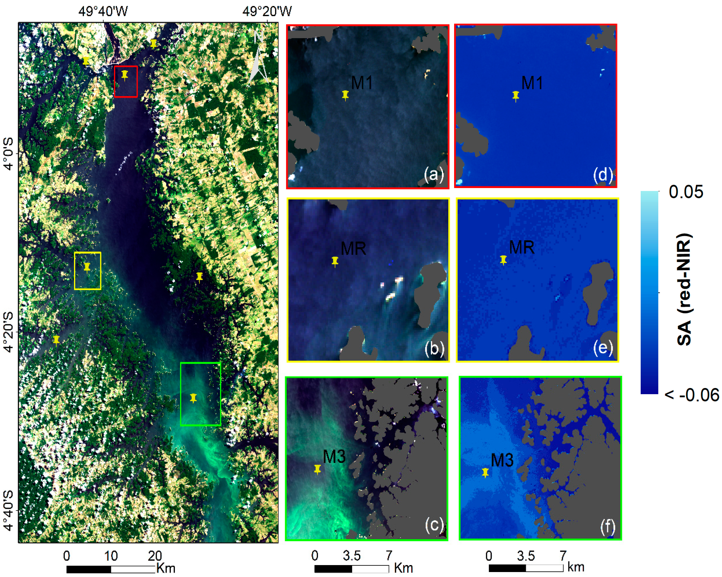
The OBPG algorithm applied to this study area showed to be able to represent the spatial dynamic of the THR in favorable weather conditions for Chl-a. The SAred-NIR algorithm could identify the algal bloom extent even in thin cloud conditions (Figure 4d). The algorithm attached higher values of SAred-NIR to areas with higher nutrients in calm weather conditions, as preferred by cyanobacteria [11].
We observed a negative correlation between Chl-a and cyanobacteria density; a result that was also observed by [37] in earlier years. In developing a trophic state index for tropical/subtropical reservoirs, De Souza Cunha et al. [69] noted poor correlation between Chl-a concentration and phytoplankton abundance. The main reason for such a poor correlation between Chl-a and phytoplankton abundance is a shift occurring between phytoplankton groups, which contributes to the total Chlorophyll-a content. This shift was reported by [70] studying algae in the Arctic, where authors reported an increase in small phytoplankton cells over larger cells, while Chl-a concentrations did not change.
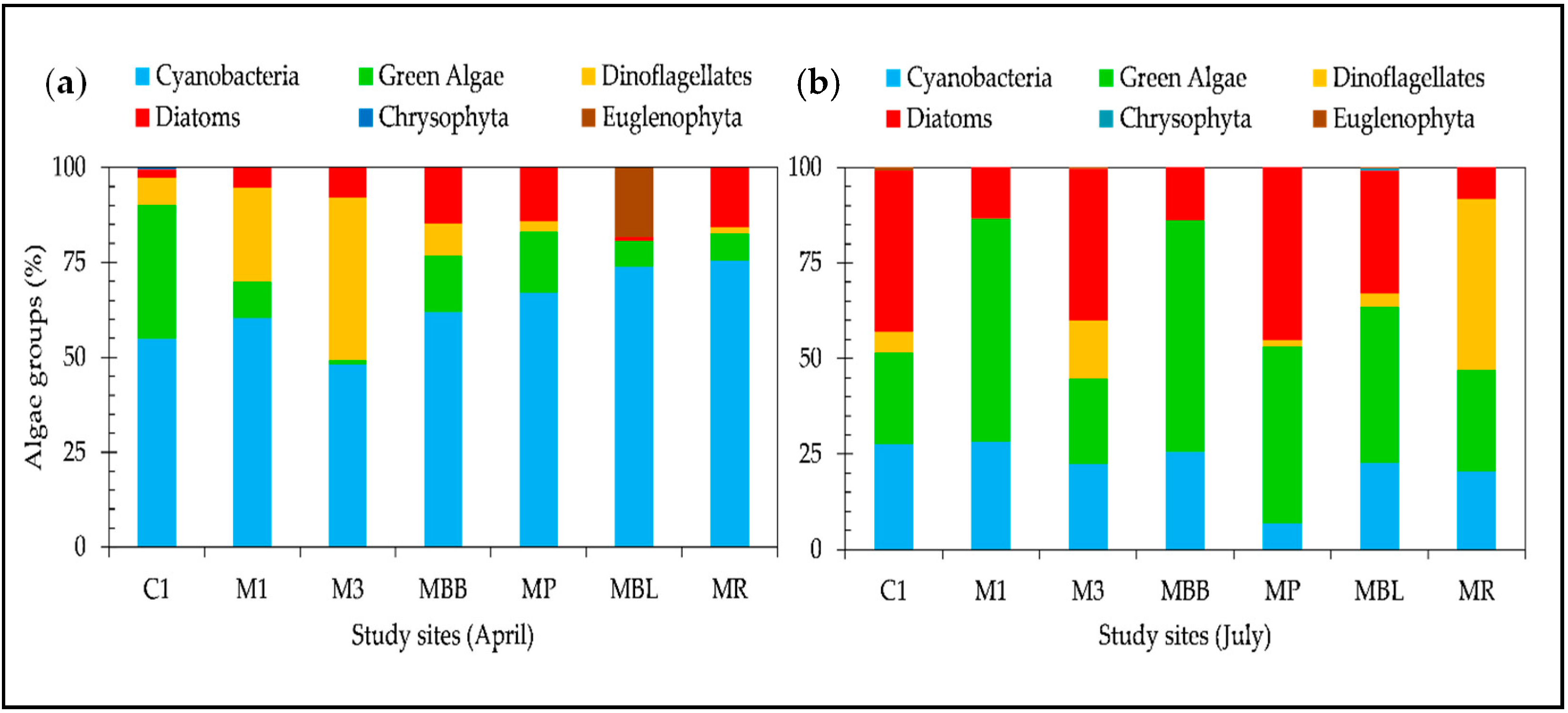
We also observed an increase in phytoplankton abundance in the lake zone (sites M1, C1 and BB), although the Chl-a concentration did not show significant variation between sites. Kasprzak et al. [71] reported shifts within the phytoplankton community related to the nutrient load during eutrophication periods. They reported a replacement of small flagellates by green algae. This may be caused by different requirements among phytoplankton species for nutrients. Due to this shifting in the phytoplankton group, caution is necessary when using Chl-a as an estimator of phytoplankton biomass [72]. Dinoflagellates and some cyanobacteria species can actually have relatively low Chlorophyll-a content per cell biovolume [73,74]. Certain cyanobacteria species, such as Dolichospermum circinalis and Microcystis aeruginosa, present protoplasm that reflects in the green region; and sometimes these species appear to be dark or brown in color with their gas-filled vesicles scattering light in the blue region [6].
Our results show an increase in density of the Nostocales order represented by the Raphidiopsis curvata species in the cyanobacteria group from April to July of 2016 (see Figures S1 and S2). We also observed an increase in nutrients such as phosphate between April and July, accompanied by an increase in silicate. Species of the Nostocales order favor turbid waters with a high phosphor concentration [75]. They are able to fix atmospheric nitrogen in low, combined inorganic sources, opening up opportunities for them to grow in low Chl-a waters classified as oligotrophic [76]. The increase in turbidity in the THR during its emptying phase is due to the increase in diatoms, which could explain the high silicate values in July [46].
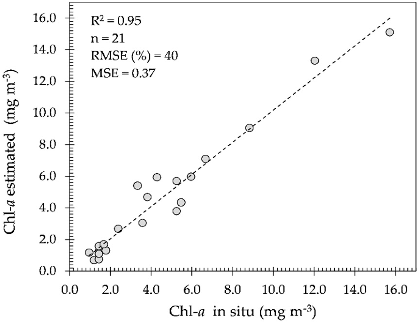
In spite of this study area being located in a cloudy region and investigated in the wet season (Figure 7a), the OBPG algorithm made a fair estimation of the Chl-a concentrations during the cloud-free period with low glint effect, corroborated with field measurements as shown in Figure 6. However, when the glint effect is high (August to September), the estimation becomes very poor. In the supplementary material, the OBPG algorithm is seen to be applied in cloud-free and low glint conditions (Figure S1). In this case, it is evident that the THR seasonally alternates between being classified as eutrophic (in April Figure 7a—full reservoir) and as meso-oligotrophic (in July Figure 7b; Figure S1—emptying reservoir).
In April, M1, MR and M3 were classified as severe bloom areas based on the SAred-NIR algorithm. The main causes were significant variation on pH levels and changes in weather conditions in temporal scale [2]. The pH level, in many aquatic systems, plays an important role regulating algal abundance and distribution as showed by [77]. Moreover, a decrease in cyanobacteria under acidified water conditions has been showed by [78,79]. We believe that it is very unlikely that the OLI sensor is capable of monitoring algal bloom in July (emptying phase) in this study area on a temporal scale. The main reason being the turbulent environment, which favors diatom biomass increase, consequently increasing turbidity and benefitting species adapted to high turbidity, such as those of the Nostocales order. Additionally, filamentous cyanobacteria, as the Notocales, may be abundant but rarely form scums in turbulent waters [80]. Turbidity increase is due to the increase in phytoplankton biomass. Scum is conductive to high reflectance in the red and NIR bands as outlined by [66] and it allows for flagging of the algal bloom extent; however, if no scum is formed, algal bloom will not be detectable using the OLI sensor.

5. Conclusions

We used ecological and optical approaches in spatial and temporal contexts to map algal bloom extent in the Tucuruí hydroelectric reservoir (THR). Our main objective was to investigate whether the combination between water limnology and satellite imagery is a suitable approach for monitoring spatial distribution and temporal frequency of algal blooms and establish their potential toxicity in the THR. Despite the fact that the ecological and optical approaches showed both drawbacks and advantages, the overall conclusion is that the OBPG algorithm is suitable for estimating the spatial and temporal variability in Chl-a concentrations. Thus, this algorithm may be applied to this study area, using OLI/L8 imagery in the periods of little cloud cover on a temporal scale and with good understanding of its water limnology.
Interestingly, the OBPG algorithm showed a fair result for this study area, which was not expected due to the use of the blue green ratio. However, the explanation for such a result might be that the oligotrophic to mesotrophic classification between July and September yielded Rrs towards the blue-green region. Additionally, this study area presents low turbidity and color concentrations from July to September as shown in the supplementary material (Figures S3 and S5).
Despite the limitations of the SAred-NIR algorithm, it showed that it is possible to flag algal bloom occurrence with some a priori knowledge of the study area and availability of limnological and remote sensing data. As the main drawback of this study was using a reduced number of satellite images, we recommend that cyanobacteria or phytoplankton studies in this area ensure that their ecological functioning is carefully considered when attempting to map occurrence using limited satellite imagery. Moreover, the goal of this study was not to quantify algal blooms directly. Instead, this approach meant to search for patterns in space and time based on their ecological preferences for conditions (such as physical, chemical and biological) that would favor algal blooms. Therefore, generated maps based on their probable occurrence would help water management decisions.
In conclusion, further study on the bio-optical properties of Amazonian reservoir waters would be beneficial to local water management in order to understand the water quality issues in these areas.

Supplementary Materials

The following are available online at www.mdpi.com/2071-1050/9/12/2194/s1, Figure S1: Maps of Chl-a concentration (mg m−3) estimated from OLI sensor using the OBPG algorithm for 16 June, 18 July and 03 August of 2013, Figure S2: Time series of Chl-a in the Tucuruí hydroelectric reservoir from 2014 to 2016, Figure S3: Time series of turbidity in the Tucuruí hydroelectric reservoir from 2014 to 2016, Figure S4: Time series of Secchi disc in the Tucuruí hydroelectric reservoir from 2014 to 2016, Figure S5: Time series of color in the Tucuruí hydroelectric reservoir from 2014 to 2016, Table S1: Cyanobacteria taxa and biovolume in percentage in April 2016, Table S2: Cyanobacteria taxa and biovolume in percentage in July 2016.

Acknowledgments

The authors would like to thank the support of Eletrobras-Eletronorte for scholarship; the Faculty of Geo-Information Science and Earth Observation (ITC) of the University of Twente; the Federal University of Pará (Brazil) for support biological analysis; the International Institute of Ecology for providing equipment for fieldwork campaigns and the Centre of environmental protection in Tucuruí for help to conduct limnological analysis. This research was carried out within a project entitled: “Development of a water quality index specific to the Amazon region”, Contract No. 4500075234 funded by Eletrobras-Eletronorte.

Author Contributions

Isabel Leidiany de Sousa Brandão wrote the article, processed the data and was involved in the fieldwork campaigns and data analysis. Chris M. Mannaerts, Wouter Verhoef and Augusto César Fonseca Saraiva gave ideas and reviewed the article. Rosildo Paiva and Elidiane V. da Silva helped conduct the phytoplankton analysis and contributed to the discussion section.

Conflicts of Interest

The authors declare no conflict of interest. The founding sponsors had no role in the design of the study; in the collection, analyses, or interpretation of data; in the writing of the manuscript, and in the decision to publish the results.

Appendix A. Atmospheric Correction of the OLI Imagery

In Appendix A Figure A1 is included which shows the processing steps of the atmospheric correction, from the OLI imagery to the final maps in this study.
Figure A1. OLI processing flow applied to the imagery of this study.
Sustainability 09 02194 g0a1
L8/OLI imagery at L1T was obtained from EarthExplorer [61] and used as input to the ACOLITE processor. In ACOLITE, atmospheric correction is performed through the advanced settings section. This section includes aerosol and Rayleigh correction options. For scenes of this study, we used NIR atmospheric correction because our samples showed turbidities lower than 30 NTU. The default is to use the SWIR band when water is moderately to extremely turbid (>30 NTU).

Appendix A.1. Chl-a Algorithm Processing Steps

To achieve the Chl-a algorithm results, level 1 images were first converted from Digital Numbers (DN) to Top Of Atmosphere radiances (TOA):
LTOA = ML × DN + AL
where, ML (multiplicative factor, gain) and AL (additive factor, offset) are values provided in the metadata file. TOA reflectances ( ρ OA) were computed according to the Equation (2):
ρ TOA = π × L T O A × d 2 F 0 × cos θ 0
where, F0 stands for extraterrestrial solar irradiance, d for sun-earth distance in Astronomical Units, and θ0 the sun zenith angle. ρ TOA is assumed to be the sum of aerosol reflectance ( ρ a). Rayleigh reflectance ( ρ r) and the water-leaving radiance reflectance just above the surface ( ρ w 0 + ) :
ρ TOA = ρ a + ρ + t × ρ w 0 +
ρ w 0 + = π × L w 0 + E d 0 +
where, E w 0 + is the water-leaving radiance, and E d 0 + the down-welling irradiance, both above the water surface. The superscript from ρ w 0 + is dropped and water-leaving radiance reflectance is referred as ρ w which was divided by π to convert into remote sensing reflectance (Rrs). More details on atmospheric correction of Landsat 8 imagery using ACOLITE is given in [56,57,59,81].

Appendix A.2. Rayleigh Corrected Reflectance

Rayleigh corrected reflectance ( ρ c) products used as input to the SAred-NIR were obtained from Rayleigh reflectance ( ρ r), which uses sun and sensor geometry. Input atmospheric conditions were atmospheric pressure (1004 hPa); Rayleigh scale factor (0.99), and site elevation (70 m). Additional options are aerosol epsilon (user defined = 1) and user defined alpha (ration of water reflectance in the re/NIR) bands) equal to 8.7 from [81].
Rayleigh-corrected reflectance ( ρ c) is obtained after subtraction of ρ c from ρ TOA with the following equation:
ρ c = ρ TOA ρ r = ρ a + t 0 t v ρ w
where, ρ r and ρ a are the reflectances resulting from Rayleigh and aerosol scattering; t0 and tv are the sun and sensor diffusive transmittances; ρ w is the water-leaving radiance reflectance.

References

  1. Johnson, N.; Revenga, C.; Echeverria, J. Managing water for people and nature. Science 2001, 292, 1071–1072. [Google Scholar] [CrossRef] [PubMed]
  2. Tundisi, J.G.; Tundisi, T.M. Limnology; CRC Press: São Paulo, Brazil, 2012. [Google Scholar]
  3. Mur, R.; Skulberg, O.M.; Utkilen, H. Cyanobacteria in the Environment: A Guide to Their Public Health Consequences, Monitoring and Management; Bartram, I.C.A.J., Ed.; WHO: London, UK, 1999; pp. 15–40. [Google Scholar]
  4. Lee, R.E. Phycology; Cambridge University Press: Cambridge, UK, 2008. [Google Scholar]
  5. De Figueiredo, D.R.; Azeiteiro, U.M.; Esteves, S.M.; Gonçalves, F.J.; Pereira, M.J. Microcystin-producing blooms—a serious global public health issue. Ecotoxicol. Environ. Saf. 2004, 59, 151–163. [Google Scholar] [CrossRef] [PubMed]
  6. Chorus, I. Cyanotoxins: Occurrence, Causes, Consequences; Springer Science & Business Media: Berlin, Germany, 2012. [Google Scholar]
  7. Sivonen, K.; Himberg, K.; Luukkainen, R.; Niemelä, S.; Poon, G.; Codd, G. Preliminary characterization of neurotoxic cyanobacteria blooms and strains from finland. Toxic. Assess. 1989, 4, 339–352. [Google Scholar] [CrossRef]
  8. Repavich, W.M.; Sonzogni, W.C.; Standridge, J.H.; Wedepohl, R.E.; Meisner, L.F. Cyanobacteria (blue-green algae) in wisconsin waters: Acute and chronic toxicity. Water Res. 1990, 24, 225–231. [Google Scholar] [CrossRef]
  9. Waxter, M.T. Analysis of Landsat Satellite Data to Monitor Water Quality Parameters in Tenmile Lake, Oregon. Master’s Thesis, Portland State University, Portland, OR, USA, 2014. [Google Scholar]
  10. Havens, K.E. Cyanobacteria blooms: Effects on aquatic ecosystems. In Cyanobacterial Harmful Algal Blooms: State of the Science and Research Needs; Springer: New York, NY, USA, 2008; pp. 733–747. [Google Scholar]
  11. Chorus, E.I.; Bartram, J. Toxic Cyanobacteria in Water: A Guide to Their Public Health Consequences, Monitoring and Management; WHO: London, UK, 1999. [Google Scholar]
  12. Randolph, K.; Wilson, J.; Tedesco, L.; Li, L.; Pascual, D.L.; Soyeux, E. Hyperspectral remote sensing of cyanobacteria in turbid productive water using optically active pigments, chlorophyll a and phycocyanin. Remote Sens. Environ. 2008, 112, 4009–4019. [Google Scholar] [CrossRef]
  13. Backer, L.C. Cyanobacterial harmful algal blooms (cyanohabs): Developing a public health response. Lake Reserv. Manag. 2002, 18, 20–31. [Google Scholar] [CrossRef]
  14. Pitois, S.; Jackson, M.; Wood, B. Problems associated with the presence of cyanobacteria in recreational and drinking waters. Int. J. Environ. Health Res. 2000, 10, 203–218. [Google Scholar] [CrossRef]
  15. Giardino, C.; Pepe, M.; Brivio, P.A.; Ghezzi, P.; Zilioli, E. Detecting chlorophyll, secchi disk depth and surface temperature in a sub-alpine lake using landsat imagery. Sci. Total Environ. 2001, 268, 19–29. [Google Scholar] [CrossRef]
  16. Koponen, S.; Pulliainen, J.; Kallio, K.; Hallikainen, M. Lake water quality classification with airborne hyperspectral spectrometer and simulated meris data. Remote Sens. Environ. 2002, 79, 51–59. [Google Scholar] [CrossRef]
  17. Kallio, K.; Kutser, T.; Hannonen, T.; Koponen, S.; Pulliainen, J.; Vepsäläinen, J.; Pyhälahti, T. Retrieval of water quality from airborne imaging spectrometry of various lake types in different seasons. Sci. Total Environ. 2001, 268, 59–77. [Google Scholar] [CrossRef]
  18. Koponen, S.; Attila, J.; Pulliainen, J.; Kallio, K.; Pyhälahti, T.; Lindfors, A.; Rasmus, K.; Hallikainen, M. A case study of airborne and satellite remote sensing of a spring bloom event in the gulf of finland. Cont. Shelf Res. 2007, 27, 228–244. [Google Scholar] [CrossRef]
  19. Strömbeck, N.; Pierson, D.C. The effects of variability in the inherent optical properties on estimations of chlorophyll a by remote sensing in swedish freshwaters. Sci. Total Environ. 2001, 268, 123–137. [Google Scholar] [CrossRef]
  20. Thiemann, S.; Kaufmann, H. Lake water quality monitoring using hyperspectral airborne data—A semiempirical multisensor and multitemporal approach for the mecklenburg lake district, germany. Remote Sens. Environ. 2002, 81, 228–237. [Google Scholar] [CrossRef]
  21. Schalles, J.F.; Yacobi, Y.Z. Remote detection and seasonal patterns of phycocyanin, carotenoid and chlorophyll pigments in eutrophic waters. Ergeb. Limnol. 2000, 55, 153–168. [Google Scholar]
  22. Dekker, A.G. Detection of Optical Water Quality Parameters for Eutrophic Waters by High Resolution Remote Sensing. Ph.D. Thesis, Vrije Universiteit, Amsterdam, The Netherland, 1993. [Google Scholar]
  23. Qi, L.; Hu, C.; Duan, H.; Cannizzaro, J.; Ma, R. A novel meris algorithm to derive cyanobacterial phycocyanin pigment concentrations in a eutrophic lake: Theoretical basis and practical considerations. Remote Sens. Environ. 2014, 154, 298–317. [Google Scholar] [CrossRef]
  24. Hunter, P.D.; Tyler, A.N.; Gilvear, D.J.; Willby, N.J. Using remote sensing to aid the assessment of human health risks from blooms of potentially toxic cyanobacteria. Environ. Sci. Technol. 2009, 43, 2627–2633. [Google Scholar] [CrossRef] [PubMed]
  25. Simis, S.G.; Peters, S.W.; Gons, H.J. Remote sensing of the cyanobacterial pigment phycocyanin in turbid inland water. Limnol. Oceanogr. 2005, 50, 237–245. [Google Scholar] [CrossRef]
  26. Hunter, P.; Tyler, A.; Willby, N.; Gilvear, D. The spatial dynamics of vertical migration by microcystis aeruginosa in a eutrophic shallow lake: A case study using high spatial resolution time-series airborne remote sensing. Limnol. Oceanogr. 2008, 53, 2391–2406. [Google Scholar] [CrossRef]
  27. Hunter, P.; Gilvear, D.; Tyler, A.; Willby, N.; Kelly, A. Mapping macrophytic vegetation in shallow lakes using the compact airborne spectrographic imager (CASI). Aquat. Conserv. Mar. Freshw. Ecosyst. 2010, 20, 717–727. [Google Scholar] [CrossRef]
  28. Vincent, R.K.; Qin, X.; McKay, R.M.L.; Miner, J.; Czajkowski, K.; Savino, J.; Bridgeman, T. Phycocyanin detection from landsat tm data for mapping cyanobacterial blooms in lake erie. Remote Sens. Environ. 2004, 89, 381–392. [Google Scholar] [CrossRef]
  29. Sun, D.; Hu, C.; Qiu, Z.; Shi, K. Estimating phycocyanin pigment concentration in productive inland waters using landsat measurements: A case study in lake dianchi. Opt. Express 2015, 23, 3055–3074. [Google Scholar] [CrossRef] [PubMed]
  30. Potes, M.; Costa, M.J.; da Silva, J.C.B.; Silva, A.M.; Morais, M. Remote sensing of water quality parameters over alqueva reservoir in the south of portugal. Int. J. Remote Sens. 2011, 32, 3373–3388. [Google Scholar] [CrossRef]
  31. Woźniak, M.; Bradtke, K.; Darecki, M.; Krężel, A. Empirical model for phycocyanin concentration estimation as an indicator of cyanobacterial bloom in the optically complex coastal waters of the baltic sea. Remote Sens. 2016, 8, 212. [Google Scholar] [CrossRef]
  32. Ogashawara, I.; Li, L.; Moreno-Madriñán, M.J. Slope algorithm to map algal blooms in inland waters for landsat 8/operational land imager images. J. Appl. Remote Sens. 2017, 11, 012005. [Google Scholar] [CrossRef]
  33. Ogashawara, I.; de Alcântara, E.H.; Stech, J.L.; Tundisi, J.G. Cyanobacteria detection in guarapiranga reservoir (São Paulo state, Brazil) using landsat tm and etm+ images. Rev. Ambient. Água 2014, 9, 224–238. [Google Scholar] [CrossRef]
  34. Pahlevan, N.; Lee, Z.; Wei, J.; Schaaf, C.B.; Schott, J.R.; Berk, A. On-orbit radiometric characterization of oli (landsat-8) for applications in aquatic remote sensing. Remote Sens. Environ. 2014, 154, 272–284. [Google Scholar] [CrossRef]
  35. Torbick, N.; Corbiere, M. A Multiscale Mapping Assessment of Lake Champlain Cyanobacterial Harmful Algal Blooms. Int. J. Environ. Res. Public Health 2015, 12, 11560–11578. [Google Scholar] [CrossRef] [PubMed]
  36. Huang, J. Detecting the Spatial Patterns of Blue-Green Algae in Harsha Lake Using Landsat 8 Imagery. Master’s Thesis, East China Normal University, Shanghai, China, 2016. [Google Scholar]
  37. Tavares, M.D.R.M. Estrutura da Comunidade Microfitoplanctônica da Área de Influência da uhe de Tucuruí-Pará. Available online: http://repositorio.ufpa.br/jspui/handle/2011/6015 (accessed on 27 November 2017).
  38. Cunha, C.J.D.S. Variação Espacial e Temporal do Fitoplâncton do Reservatório da Usina Hidrelétrica de Tucuruí-Pará. Master’s Thesis, Universidade Federal do Pará, Belém, Brazil, 2013. [Google Scholar]
  39. International Ocean-Colour Coordinating Group (IOCCG). Ocean-Color Observations from a Geostationary Orbit; IOCCG: Dartmouth, NS, Canada, 2012; p. 110. [Google Scholar]
  40. Reynolds, C.S.; Huszar, V.; Kruk, C.; Naselli-Flores, L.; Melo, S. Towards a functional classification of the freshwater phytoplankton. J. Plankton Res. 2002, 24, 417–428. [Google Scholar] [CrossRef]
  41. Tundisi, J.G.; Santos, M.A.; Menezes, C.F.S. Experience and Lessons Learned Brief—Lbmi Project—Tucurui Hydroelectric Power Plant; World Lake Database, International Lake Envrionment Committee Foundation (ILEC): Shiga, Japan, 2006. [Google Scholar]
  42. Da Costa Lobato, T.; Hauser-Davis, R.A.; de Oliveira, T.F.; Maciel, M.C.; Tavares, M.R.M.; da Silveira, A.M.; Saraiva, A.C.F. Categorization of the trophic status of a hydroelectric power plant reservoir in the brazilian amazon by statistical analyses and fuzzy approaches. Sci. Total Environ. 2015, 506–507, 613–620. [Google Scholar] [CrossRef] [PubMed]
  43. Espíndola, E.L.G.; Matsumura-Tundisi, T.; Rietzler, A.C.; Tundisi, J.G. Spatial heterogeneity of the tucuruí reservoir (state of Pará, Amazonia, Brazil) and the distribution of zooplanktonic species. Rev. Bras. Biol. 2000, 60, 179–194. [Google Scholar] [CrossRef] [PubMed]
  44. Noernberg, M.A.; de Moraes Novo, E.M.L.; Krug, T. Radar system application for the management of aquatic plant infestation in reservoirs: Advantages and disadvantages. Bol. Ciênc. Geod. 1999, 5, 41–54. [Google Scholar]
  45. Ideflor-Bio. Reserva de Desenvolvimento Sustentável Alcobaça. Available online: http://ideflorbio.pa.gov.br/unidades-de-conservacao/regiao-administrativa-tucurui/reserva-de-desenvolvimento-sustentavel-alcobaca/ (accessed on 1 March 2017).
  46. De Sousa Brandao, I.L.; Mannaerts, C.M.; Saraiva, A.C.F. Seasonal variation of phytoplankton indicates small impacts of anthropic activities in a brazilian amazonian reserve. Ecohydrol. Hydrobiol. 2017, 17, 217–226. [Google Scholar] [CrossRef]
  47. Golterman, H.L.; Clymo, R.S.; Ohnstad, M.A.M. Methods for Physical and Chemical Analysis of Fresh Waters; Blackwell Scientific: Wageningen, The Netherlands, 1978. [Google Scholar]
  48. Utermöhl, H. Zur vervollkommnung der quantitativen phytoplankton-methodik. Mitt. Int. Ver. Theor. Angew. Limnol. 1958, 9, 1–38. [Google Scholar]
  49. Desikachary, T. Cyanophyta Indian Council of Agricultural Research New Delhi, India; Indian Council of Agricultural Research: New Delhi, India, 1959. [Google Scholar]
  50. Hillebrand, H.; Dürselen, C.-D.; Kirschtel, D.; Pollingher, U.; Zohary, T. Biovolume calculation for pelagic and benthic microalgae. J. Phycol. 1999, 35, 403–424. [Google Scholar] [CrossRef]
  51. Wetzel, R.G.; Likens, G.E. Composition and biomass of phytoplankton. In Limnological Analyses; Wetzel, R.G., Likens, G.E., Eds.; Springer: New York, NY, USA, 2000; pp. 147–174. [Google Scholar]
  52. R Development Core Team. R: A Language and Environment for Statistical Computing; R Foundation for Statistical Computing: Vienna, Austria, 2010. [Google Scholar]
  53. Kutser, T.; Pierson, D.C.; Kallio, K.Y.; Reinart, A.; Sobek, S. Mapping lake cdom by satellite remote sensing. Remote Sens. Environ. 2005, 94, 535–540. [Google Scholar] [CrossRef]
  54. Perkins, T.; Adler-Golden, S.; Matthew, M.W.; Berk, A.; Bernstein, L.S.; Lee, J.; Fox, M. Speed and accuracy improvements in flaash atmospheric correction of hyperspectral imagery. Opt. Eng. 2012, 51, 111707. [Google Scholar] [CrossRef]
  55. Gordon, H.R.; Wang, M. Retrieval of water-leaving radiance and aerosol optical thickness over the oceans with seawifs: A preliminary algorithm. Appl. Opt. 1994, 33, 443–452. [Google Scholar] [CrossRef] [PubMed]
  56. Vanhellemont, Q.; Ruddick, K. Turbid wakes associated with offshore wind turbines observed with landsat 8. Remote Sens. Environ. 2014, 145, 105–115. [Google Scholar] [CrossRef]
  57. Vanhellemont, Q.; Ruddick, K. Advantages of high quality swir bands for ocean colour processing: Examples from landsat-8. Remote Sens. Environ. 2015, 161, 89–106. [Google Scholar] [CrossRef]
  58. Vermote, E.; Tanré, D.; Deuzé, J.; Herman, M.; Morcrette, J.; Kotchenova, S. Second simulation of a satellite signal in the solar spectrum-vector (6sv). Appl. Opt. 2006, 45, 6762–6774. [Google Scholar]
  59. Vanhellemont, Q.; Ruddick, K. Acolite for Sentinel-2: Aquatic Applications of MSI Imagery; Living Planet Symposium; Ouwehand, L., Ed.; ESA Communications: Noordwijk, The Netherlands, 2016. [Google Scholar]
  60. Franz, B.A.; Bailey, S.W.; Kuring, N.; Werdell, P.J. Ocean color measurements with the operational land imager on landsat-8: Implementation and evaluation in seadas. J. Appl. Remote Sens. 2015, 9, 096070. [Google Scholar] [CrossRef]
  61. USGS. Earth Explorer. Available online: http://earthexplorer.usgs.gov/ (accessed on 3 April 2017).
  62. Hu, C. A novel ocean color index to detect floating algae in the global oceans. Remote Sens. Environ. 2009, 113, 2118–2129. [Google Scholar] [CrossRef]
  63. Kirk, J.T.O. Light and Photosynthesis in Aquatic Ecosystems; Cambridge university press: Cambridge, UK, 1994; p. 509. [Google Scholar]
  64. Tundisi, J.G.; Matsumura-Tundisi, T.; Abe, D.S. Climate monitoring before and during limnological studies: A needed integration. Braz. J. Biol. 2007, 67, 795–796. [Google Scholar] [CrossRef] [PubMed]
  65. Curtarelli, M.P.; Ogashawara, I.; de Araújo, C.A.S.; Lorenzzetti, J.A.; Leão, J.A.D.; Alcântara, E.; Stech, J.L. Carbon dioxide emissions from tucuruí reservoir (Amazon Biome): New findings based on three-dimensional ecological model simulations. Sci. Total Environ. 2016, 551, 676–694. [Google Scholar] [CrossRef] [PubMed]
  66. Pettersson, L.H.; Pozdnyakov, D. Monitoring of haRmful Algal Blooms; Springer Science & Business Media: Chichester, UK, 2012. [Google Scholar]
  67. Tundisi, J.G.; Goldemberg, J.; Matsumura-Tundisi, T.; Saraiva, A.C.F. How many more dams in the amazon? Energy Policy 2014, 74, 703–708. [Google Scholar] [CrossRef]
  68. Chapman, D. Water Quality Assessment—A Guide to the Use of Biota, Sediments and Water in Environmental Monitoring; CRC Press: New York, NY, USA, 2016. [Google Scholar]
  69. De Souza Cunha, E.D.; da Cunha, A.C.; da Silveira, A.M., Jr.; Faustino, S.M.M. Phytoplankton of two rivers in the eastern amazon: Characterization of biodiversity and new occurrences. Acta Bot. Bras. 2013, 27, 364–377. [Google Scholar] [CrossRef]
  70. Li, W.K.; McLaughlin, F.A.; Lovejoy, C.; Carmack, E.C. Smallest algae thrive as the arctic ocean freshens. Science 2009, 326, 539. [Google Scholar] [CrossRef] [PubMed]
  71. Kasprzak, P.; Padisák, J.; Koschel, R.; Krienitz, L.; Gervais, F. Chlorophyll a concentration across a trophic gradient of lakes: An estimator of phytoplankton biomass? Limnol. Ecol. Manag. Inland Waters 2008, 38, 327–338. [Google Scholar] [CrossRef]
  72. Felip, M.; Catalan, J. The relationship between phytoplankton biovolume and chlorophyll in a deep oligotrophic lake: Decoupling in their spatial and temporal maxima. J. Plankton Res. 2000, 22, 91–106. [Google Scholar] [CrossRef]
  73. Cunha, D.G.F.; do Carmo Calijuri, M.; Lamparelli, M.C. A trophic state index for tropical/subtropical reservoirs (Tsi Tsr). Ecol. Eng. 2013, 60, 126–134. [Google Scholar] [CrossRef]
  74. Vargas, S.R. Influência da Concentração de Nutrientes na Interação Entre Duas Espécies Fitoplanctônicas Isoladas do Reservatório de Itupararanga-SP. Master’s Thsis, Universidade de São Paulo, São Paulo, Brazil, 2012. [Google Scholar]
  75. Chorus, I.; Bartram, J. Toxic Cyanobacteria in Water; Taylor & Francis: London, UK, 2002. [Google Scholar]
  76. Sukenik, A.; Hadas, O.; Kaplan, A.; Quesada, A. Invasion of nostocales (cyanobacteria) to subtropical and temperate freshwater lakes—Physiological, regional, and global driving forces. Front. Microbiol. 2012, 3, 86. [Google Scholar] [CrossRef] [PubMed]
  77. Chenl, Y. Effects of PH on the Growth and Carbon Uptake of Marine Phytoplankton. Mar. Ecol. Prog. Ser. 1994, 109, 83–94. [Google Scholar] [CrossRef]
  78. Eichner, M.; Rost, B.; Kranz, S.A. Diversity of ocean acidification effects on marine n 2 fixers. J. Exp. Mar. Biol. Ecol. 2014, 457, 199–207. [Google Scholar] [CrossRef] [Green Version]
  79. Yamamoto, Y.; Nakahara, H. The formation and degradation of cyanobacterium aphanizomenon flos-aquae blooms: The importance of ph, water temperature, and day length. Limnology 2005, 6, 1–6. [Google Scholar] [CrossRef]
  80. Reynolds, C.S. The Ecology of Phytoplankton; Cambridge University Press: New York, NY, USA, 2006. [Google Scholar]
  81. Ruddick, K.; Vanhellemont, Q.; Dogliotti, A.; Nechad, B.; Pringle, N.; Van der Zande, D. New Opportunities and Challenges for High Resolution Remote Sensing of Water Colour. In Proceedings of the Ocean Optics XXIII, Victoria, BC, Canada, 23–28 October 2016. [Google Scholar]
Figure 1. Study area with: (a) sampling sites and (b) monthly rainfall from January 2014 to December 2016.
Sustainability 09 02194 g001
Figure 2. Contribution of algae groups to the total biovolume in relative percentage. (a) Study sites (April); (b) Study sites (July).
Sustainability 09 02194 g002
Figure 3. Rayleigh corrected reflectance ( ρ c) collected in (a) April and (b) July, 2016.
Sustainability 09 02194 g003
Figure 4. Locations where the SAred-NIR algorithm was applied: (a) M1 site; (b) MR; (c) M3 site with algal bloom indication. The scene is LC82240632016112LGN01 (April 2016) in false color (R = 665 nm, G = 561 nm, B = 483 nm); (df) are SAred-NIR classifications.
Sustainability 09 02194 g004
Figure 5. Location where the SAred-NIR algorithm was applied: (c) M3 site with algal bloom indication and other sites (a,b,d,e) without bloom indication. The scene is LC82240632016208LGN01 (July 2016) in false color (R = 665 nm, G = 561 nm, B = 483 nm); (f) SAred-NIR classification.
Sustainability 09 02194 g005
Figure 6. Chl-a estimated with the Ocean Biology Processing Group (OBPG) algorithm.
Sustainability 09 02194 g006
Figure 7. Maps of Chl-a concentrations (mg m−3) estimated using the OLI sensor and the OBPG algorithm for (a) April 21, and (b) July 26 of 2016, respectively.
Sustainability 09 02194 g007
Table 1. L8/Operational Land Imager (OLI) bands with wavelength and ground sampling distance (GSD).
BandWavelength (nm) RangeGSD (m)
1 (Coastal/aerosol)433–45330
2 (Blue)450–51530
3 (Green)525–60030
4 (Red)630–68030
5 (NIR)845–88530
6 (SWIR 1)1560–166030
7 (SWIR 2)2100–230030
8 (PAN)500–68015
9 (CIRRUS)1360–139030
Table 2. Main characteristics of algal blooms according to [32].
CharacteristicsSevere Bloom (SB)Moderate Bloom (MB)
Water surface layerCharacterized by a thick scum of algaeNo scums but is visible in the surface layer
Cyanobacteria counts (cell L−1)≥100,00010,000–100,000
ToxinsPresence of cyanotoxin
Biovolume (mm3 L−1)≥101–10
Chl-a (µg L−1)≥505–10
SAred-NIR>0.15−0.05–0.15
Table 3. Summary of error analysis used in this study.
EstimatorEquations
MSE 1 n i = 1 n ( x i estimated x i measured ) 2
MAPE { mean   ( 1 n i = 1 n | x i estimated x i measured x i measured | ) } × 100 %
RMSE RMSE = MSE
bias 1 n i = 1 n ( x i estimated x i measured )
MNB 100 n i = 1 n | x i estimated x i measured x i measured |
Table 4. Environmental characteristics of the sample sites of the study area.
Sites (Spatial Perspective)Local CharacteristicsFunctional Groups (Ecological Perpective)
April to July
M3River zonePB
MPUCTransition zoneMB
MBELTransition zoneGNA
MRTransition zoneM
M1LakeMF
BBLakePB
C1LakeH1MP
Table 5. Descriptive statistics of the water quality parameters measured in (a) April and (b) July, 2016. Statistical metrics include: minimum value (Min), maximum value (Max), average, standard deviation (SD) and coefficient of variation (CV) in percentages (%).
a. Dataset Measured on April 2016 at 7 Sites
ParameterMinMaxAverageSDCV (%)
DO (mg L−1)4.246.225.530.529.35
Temperature (°C)29.2830.9129.730.521.75
pH7.558.677.870.303.77
Suspended solids (mg L−1)0.203.001.431.0069.80
Transparency (m)1.103.101.860.6736.30
EC (µs/s)36.3040.6037.651.413.74
Nitrate (mg L−1)0.000.050.020.0282.02
Ion ammonium (mg L−1)0.020.290.110.12107.25
Phosphate (µg L−1)0.000.010.010.0058.37
Silicate (mg L−1)1.905.014.041.0826.79
Chl-a (mg m−3)2.3458.5413.4414.78110.00
b. Dataset Measured on July 2016 at 7 Sites
ParameterMinMaxAverageSDCV (%)
DO (mg L−1)4.627.145.570.8214.78
Temperature (°C)29.5431.6030.550.682.22
pH6.977.207.070.071.04
Suspended solids (mg L−1)0.201.100.590.3253.74
Transparency (m)1.604.502.500.8533.81
EC (µs/s)13.0041.3026.2610.1238.54
Nitrate (mg L−1)0.010.440.160.1590.49
Ion ammonium (mg L−1)0.020.470.160.1377.26
Phosphate (mg L−1)0.000.060.010.02132.64
Silicate (mg L−1)7.048.167.770.384.92
Chl-a (mg m−3)0.898.502.592.4795.64
Table 6. Error analysis results.
ParameterRMSE (%)MAPE (%)BiasMNB (%)
Chl-a (mg m−3)4031.970.3713.46

