Dismantling of the Inverted U-Curve of Open Innovation
by
 ,
,
JinHyo Joseph Yun
1,*, 
DongKyu Won
2,
EuiSeob Jeong
2,
KyungBae Park
3,
DooSeok Lee
1 and
Tan Yigitcanlar
4
1
Daegu Gyeongbuk Institute of Science and Technology (DGIST), 333, Techno Jungang Daero, Hyeonpung-Myeon, Dalseong-Gun, Daegu 42988, Korea
2
Korea Institute of Science and Technology Information (KISTI), 66, Hoegi-ro, Dongdaemun-gu, Seoul 02456, Korea
3
Department of Business Administration, Sangji University, 83 Sangjidae-gil, Wonju, Gangwon 26339, Korea
4
School of Civil Engineering and Built Environment, Queensland University of Technology (QUT), 2 George Street, Brisbane, QLD 4001, Australia
*
Author to whom correspondence should be addressed.
Sustainability 2017, 9(8), 1423; https://0-doi-org.brum.beds.ac.uk/10.3390/su9081423
Submission received: 3 July 2017
/
Revised: 4 August 2017
/
Accepted: 9 August 2017
/
Published: 11 August 2017
(This article belongs to the Special Issue Sustainability of Economic Growth: Combining Technology, Market and Society)
Abstract
:The purpose of this study is to address the following research question: What is the relationship between open innovation and firm performance? The study built up a research framework with three factors—i.e., open innovation strategy, time scope, and industry condition—to find out the concrete open innovation effects on firm performance. This study adopted four different research methods. Firstly, we applied the aforementioned factors to a game of life simulation in order to identify the concrete differences of open innovation effects on firm performance. Secondly, the study examined the real dynamics of open innovation effects on firm performance in the aircraft industry—one of the oldest modern industries—through a quantitative patent analysis. It then looked into the effects of major factors that impact open innovation effects. Thirdly, this study developed a mathematical model and tried to open the black box of open innovation effects on firm performance. Lastly, the study logically compiled research on open innovation effects on firm performance through the presentation of a causal loop model and derived the possible implications.
1. Introduction
The fourth industrial revolution era is upon us [1,2]. New open connections and the combination of technology and market are among the key success factors of this era. Open connections and the combination of technology and market generate open innovation. Even though open innovation has become more important in the fourth industrial revolution, the relation between open innovation and firm performance has not manifested until now. Therefore, it is important to understand the effects of open innovation on firm performance to be able to respond to the fourth industrial revolution.
With the emergence of the global knowledge–based economy, open connections of markets with technologies existing in the world are becoming an important decision factor in the growth of businesses models, regional innovation systems (RIS), and national innovation systems (NIS) [3]. Although open innovation research has become active in various areas throughout the globe following the publication of a book on the subject by Chesbrough in 2003, this study focuses on the effect of open innovation—an area where sufficient research has not been carried out yet. Numerous studies on the effects of open innovation—the relationship between the performance and the activation of the open innovation of firms—is represented by an inverted U-curve according to a number of studies [4,5,6]. Despite the findings of these works, there is not much concretion of research on the specific decision factors and contents of the inverted U-curve, and this is an understudied research topic. Until now, many statistical studies on open innovation revealed that the relation between open innovation and firm performance has an inverted U-curve relation [6]. However, in several case studies it was indicated that the diverse relations between open innovation and firm performance can occur depending on the situation [7,8].
The purpose of this study is to address the following research question: What is the relation between open innovation and firm performance? This question aims to depict whether an inverted U-curve relationship exists.
2. Materials and Methods
2.1. Literarure Review
As the interest in research with empirical evidence on open innovation and innovation performance increases, more attention has been paid on the inverted U-curve relation between the breadth and depth of research through external sources of innovation and firm performance [6,9,10,11]. However, according to the firm size, open innovation effects on firm performance are different [4,5,6]. Smaller firms and less research and development (R&D) intensive firms opt for close strategies, and medium-sized firms and firms with medium R&D intensity opt for open strategies [12]. On average, medium-sized firms are more heavily involved in open innovation than their smaller counterparts [8]. Therefore, small and medium sized enterprises (SMEs) can have five different open innovation strategies. These are closed innovator, supply-chain searcher, technology-oriented searcher, application-oriented searcher, demand-driven searcher, and full-scope searcher [13]. In addition, open innovation in SMEs can perform innovative performance in the situated intermediated network models [14]. In fact, different open innovation activities are beneficial for different innovation outcomes. Technology sourcing is linked to radical innovation performance, and technology scouting is linked to incremental innovation performance [6]. Similarly, open innovation in technology development, open innovation in product development, open innovation in manufacture, and open innovation in commercialization produces different firm performance innovation [15].
According to the literature, there exists an inverted U-curve relation but at the same time something more could be in the relationship between open innovation and performance [16,17,18,19,20]. There are key factors such as firm size, sector that the company belongs to, R&D, or absorptive capacity, which give effects to open innovation effects on firm performance [12]. In addition to this, there are several factors that have effects on a firm’s openness decisions in innovation such as a lack of market and technological knowledge, ineffective intellectual property protection mechanisms, competitors’ threats, and firm’s need for financial funding [8]. In the case of SMEs customer demands, or competitors also affect the open innovation effects [13]. SMEs choose different open innovation strategies according to their organizational context, internal requirements, and ability to improve innovation performance, which will affects to the open innovation effects [14]. In leveraging external sources of innovation, there can be the difference in open innovation effects according to the four-phases such as obtaining, integrating, commercializing, and interaction [21]. For example, according to the knowledge condition, the benefits of open innovation practices are different for food and beverage firms as compared to others [15].
2.2. Research Framework
The inverted U-curve sheds light on the relationship between the breadth and depth of external sources of innovation and innovative performance [6]. Another research studies indicated that firms’ pursue strategies of close innovation, open innovation, and semi-open innovation in accordance with the growth of the business [4]. Both quantitatively explain that the effect of open innovation does not grow infinitely, but has a limit [15]. Moreover, in several aspects—such as different open innovation activities, different open innovation intermediated networks of SMEs, different open innovation strategies, and four phases of searching knowledge models—literature reviews discuss the intensity of open innovation as a strategy of firms. Firms choose open innovation intensity strategies in the industry to which they belong, as well as the located time condition.
The extent of knowledge amount—including the stages of technological development, product development, manufacturing, and commercialization—the degree of technological knowledge, and the different open innovation strategy, are being expressed in various forms [16]. The difference of knowledge amount of the industry a firm belongs to, as well as its sector, regional innovation system, or national innovation, is equated with the environment conditions of the firm. Besides, time diversely appears in the literature reviews, such as the four-phase model, in leveraging external sources of innovation, changes in business volume and business innovation, or various time contexts of technological innovation [17].
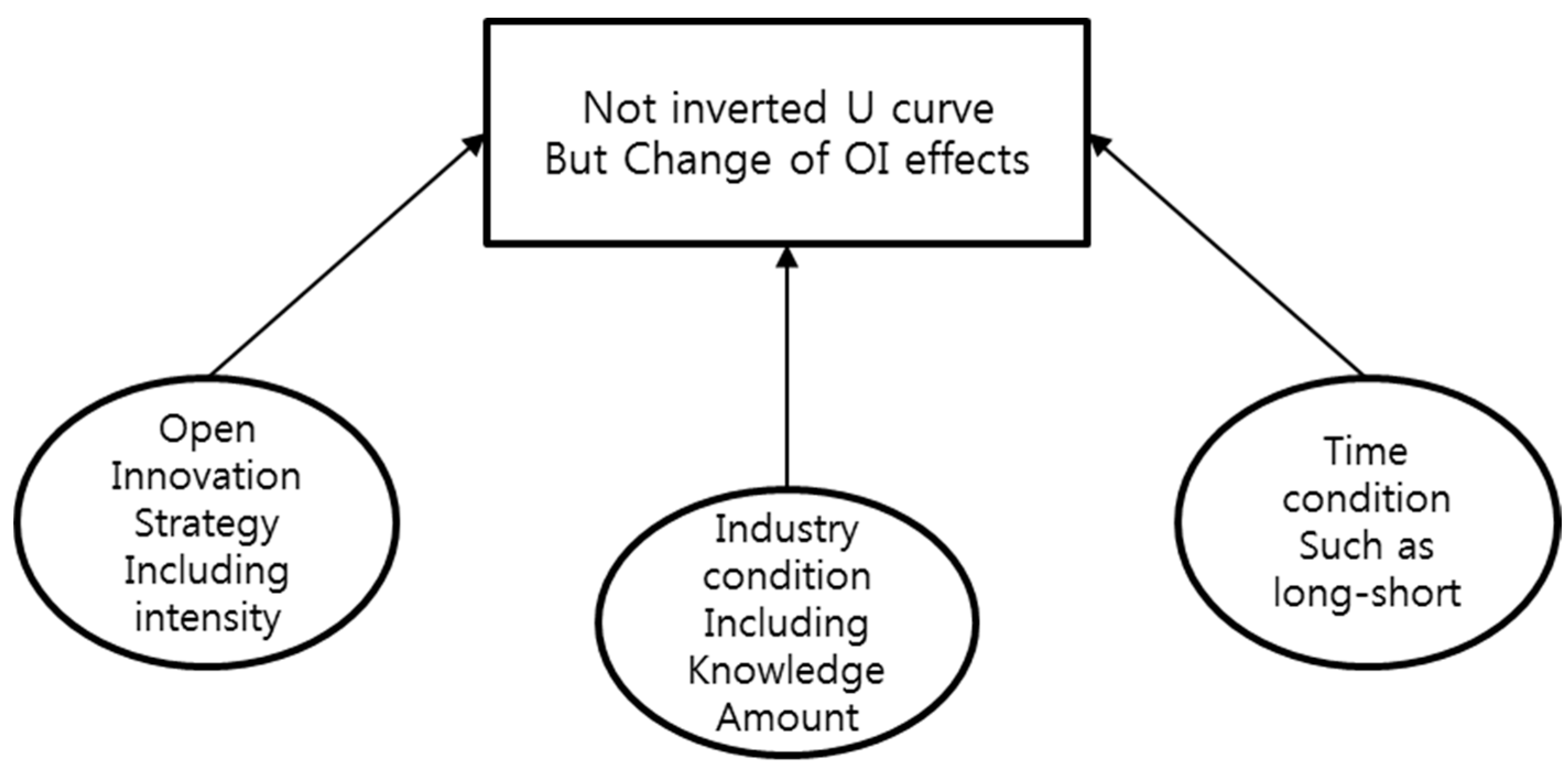
In the case open innovation belongs to different categories such as inbound actions, outbound actions, coupled actions, and internal open innovation actions, open innovation effects on firm performance can be different such as plus (+), minus (−), or inverted U-curve [10]. By examining previous research work on open innovation—quantitative studies in particular—a quantitative relation model between open innovation and the firms’ performance can be established with open innovation intensity, knowledge amount, and time. These have influence on the inverted U-curve, and change of open innovation effects (i.e., performance with the limitation of open innovation), as in the research model shown in Figure 1.
2.3. Research Methods and Scope
Firstly, this research will undertake a game of simulation to show the diversity of open innovation effects. At this the game of life model will be built from research frame which has bases on literature review. Secondly, the study will reveal the dynamics of open innovation and open innovation effects from aircraft industry. In order to do so it will analyze the aircraft industry patents from the perspective of research framework. Thirdly, it will build mathematical model of the open innovation effect, which is based on the research framework, and simulate the open innovation effects. Lastly, the study will build the causal loop model on the open innovation effects, which is based on the research framework, and explain the three major factors in the research framework. With these four research steps, the study will reveal the diverse and dynamic open innovation effect.
3. Game of Life Simulation of Open Innovation Effects
This section concretely materializes the simulations through changes in the game of life model. A number of previous studies have simulated dynamics through the game of life model, using the statistical mechanics of a dynamic system based on Conway’s game of life, including a stochastic cellular automata model of innovation [19,20,22]. Through the game of life model, three-dimensional simulations are carried out (i.e., knowledge amount, open innovation intensity, and time) [23,24], and through the implementation of the logical functions in the game of life, the researchers were able to simulate eight conditions of open innovation. Moreover, the effect of boundary conditions on scaling in the game of life can be materialized in this simulation [25,26]. This study thus proceeded with simulations using the current game of life model that Conway proposed as the base [20].
In the game of life, humans cannot control the ‘game’. The initial pattern constitutes the seed of the entire system of the game. In the game of life, future results are decided based on initial conditions. Initial conditions can be decided for future results. Thus, random initial conditions are confirmed by algorism—a random-based zero-player game where the structure of the game cannot be changed during the game [26].
If simulation conditions were organized based on Figure 1, eight types of simulations could be deducted, which are shown in Table 1. Through the interpretation of the eight-simulation model results that could be applicable in real life, a more concrete, overall understanding of the specific open innovation strategy and the business performance it brings about will become possible by suggesting in advance the various situations where open innovation effects under the eight conditions can actually appear.
The study draws three parameters such as the level of open innovation, time scope, and knowledge condition of the specific industry as follows. Firstly, when neighbors are three agents, a new agent is born; when neighbors are less than two or more than three agents, a corresponding agent dies. These conditions of the traditional game of life are deemed low open innovation. When neighbors are two agents, a new agent is born; when neighbors are less than one or more than two agents, a corresponding agent dies. These are presumed to be high open innovation. Secondly, when the initial knowledge was small, the patent number of the US aircraft industry in 1970 was presumed to have an initial value of 251. On the contrary, in cases when the initial knowledge was large, the patent number of the US aircraft industry in 2000 was presumed to be 419. This study conceptualizes high open innovation and low open innovation as high living with a low neighborhood, and low living even a high neighborhood respectively at the game of life model. Thirdly, the short term presupposes 120 ticks, which means one year. On the other hand, the long term presupposes 1200 ticks, which means 10 years.
In Figure 2, Case A is a low open innovation, with a short-term and low knowledge condition. However, it showed that agents increased even after the target time agents decreased. Case B is also a low open innovation but with a long-term and small knowledge condition. Here, the agents increased at the starting time, but decreased at the long-term target and fluctuated. In the end, Case A showed an inverted U-curve. Case C, as a high open innovation with a short-term and small knowledge condition—as well as Case D, as a high open innovation with a long-term and small knowledge condition—showed that agents increased and fluctuated with the same pattern, following a similar boundary with high complexity compared to A and B. As such, it can be seen that the complexity of Cases A and B is small or medium, whereas Cases C and D have high complexity.
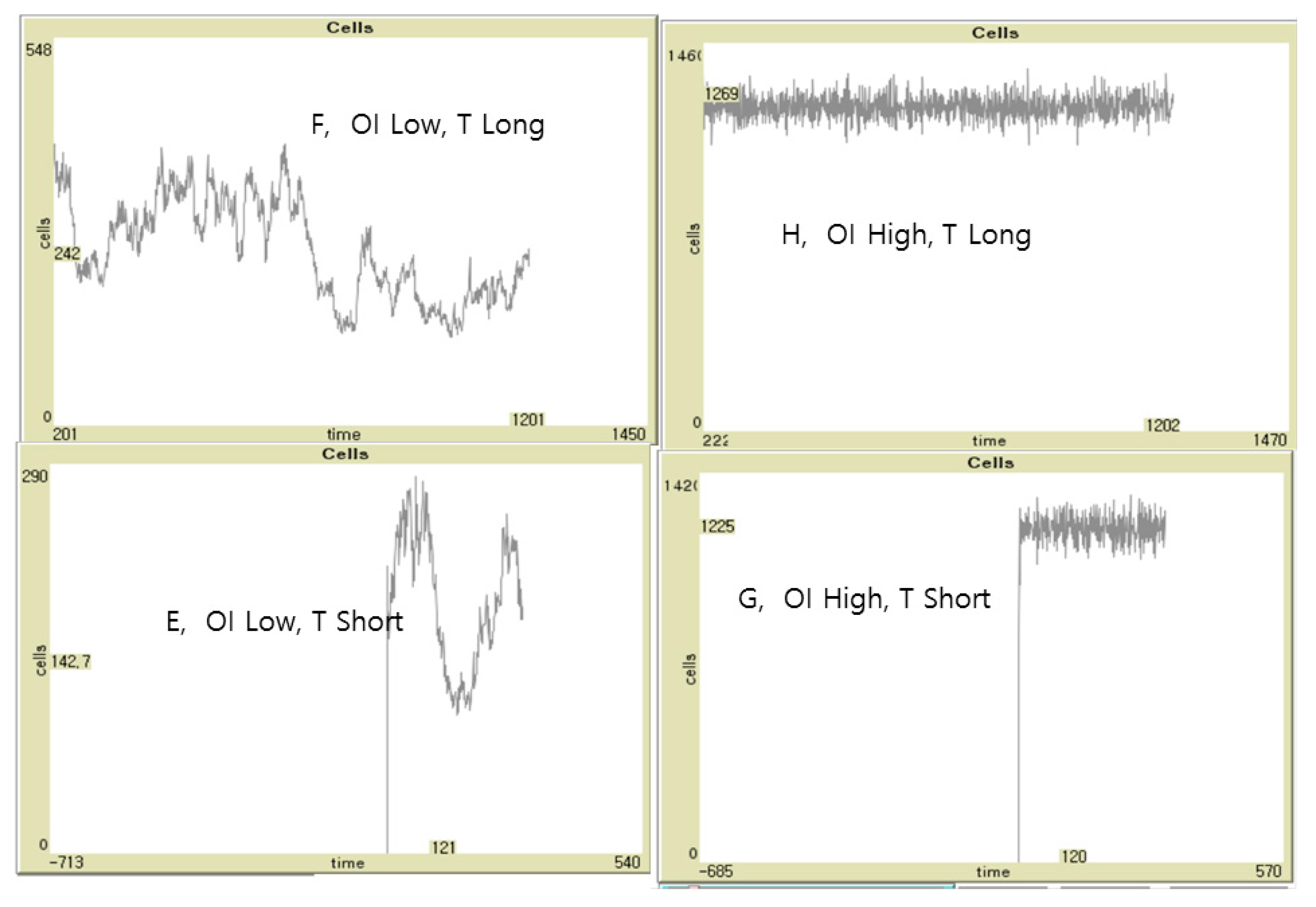
Figure 3 shows the four simulation results of the case when the initial knowledge condition is high. In Case E, as a low open innovation with a short-term and high knowledge condition, and Case F, as a low open innovation with a long-term and high knowledge condition, the agents have medium complexity, showing an inverted U-curve. In Case G, as a high open innovation with a short-term and high knowledge condition, as well as Case H, as a high open innovation with a long-term and high knowledge condition, the agents are in a very complex situation with a double-sized boundary, compared to the low knowledge condition after increasing at the starting point.
Comparing the complexity of the eight cases, the following can thus be seen: G, H > C, D > E, F > A, B. According to the game of life simulation, an increase in agents—that is, open innovation results—correlates with an increase in complexity. This means that high open innovation cannot confirm high results.
4. Real Dynamics of Open Innovation Effects in the Aircraft Industry
In this section, the real dynamics of open innovation and performance under several conditions—such as long- and short-term conditions, small and large knowledge conditions, and high and low open innovation—will be discussed. For this purpose, the researchers performed a patent analysis of the aircraft industry. Patent data were collected by searching keywords from the constructed Global Patent Analysis Service System (GPASS) database of the Korea Institute of Science and Technology Information (KISTI). GPASS has 88,674,540 patents from 77 nations and organizations, including the EU and WIPO (as of 15 February 2015). In this study, US patent data related to the aircraft industry were used to analyze the real dynamics of open innovation and performance.
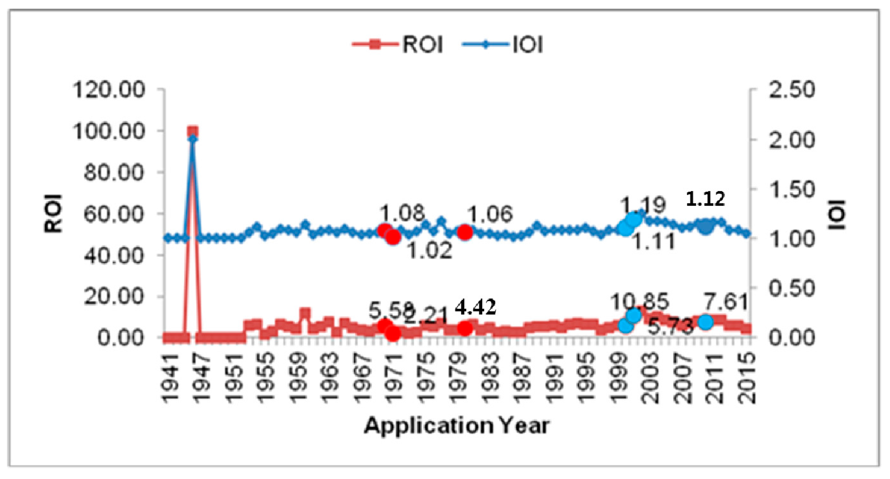
Based on Figure 4, the ratio of open innovation (ROI)—i.e., the width of open innovation—which signifies the ratio of jointly applied patents among all other patents, generally underwent fluctuations, but an overall increase was achieved, although it faltered slightly in the late 2000s [27]. The intensity of open innovation (IOI)—i.e., the depth of open innovation—which signifies the average number of joint applications per patent, also saw fluctuations and began to show faint signs of slowing down near 2010.
According to Figure 5, open innovations in a low knowledge condition showed a short-term decrease between 1970 and 1971 and a long-term decrease between 1970 and 1980 with regard to the depth and breadth of open innovation. Contrary to this, open innovation in a high knowledge condition showed a short-term increase between 2000 and 2001 and a long-term decrease between 2000 and 2010 with regard to the depth and breadth of open innovation. If the time period of 1970 to 1980 is accepted as a low knowledge society, 2000 to 2010 as a high knowledge society, and one year as the short term and 10 years as the long term, the following is true. According to aircraft industry patents, with respect to open innovation dynamics, open innovation in the low knowledge society decreased in both the short term and the long term. In contrast, open innovation in the high knowledge society both increased in the short term and the long term.
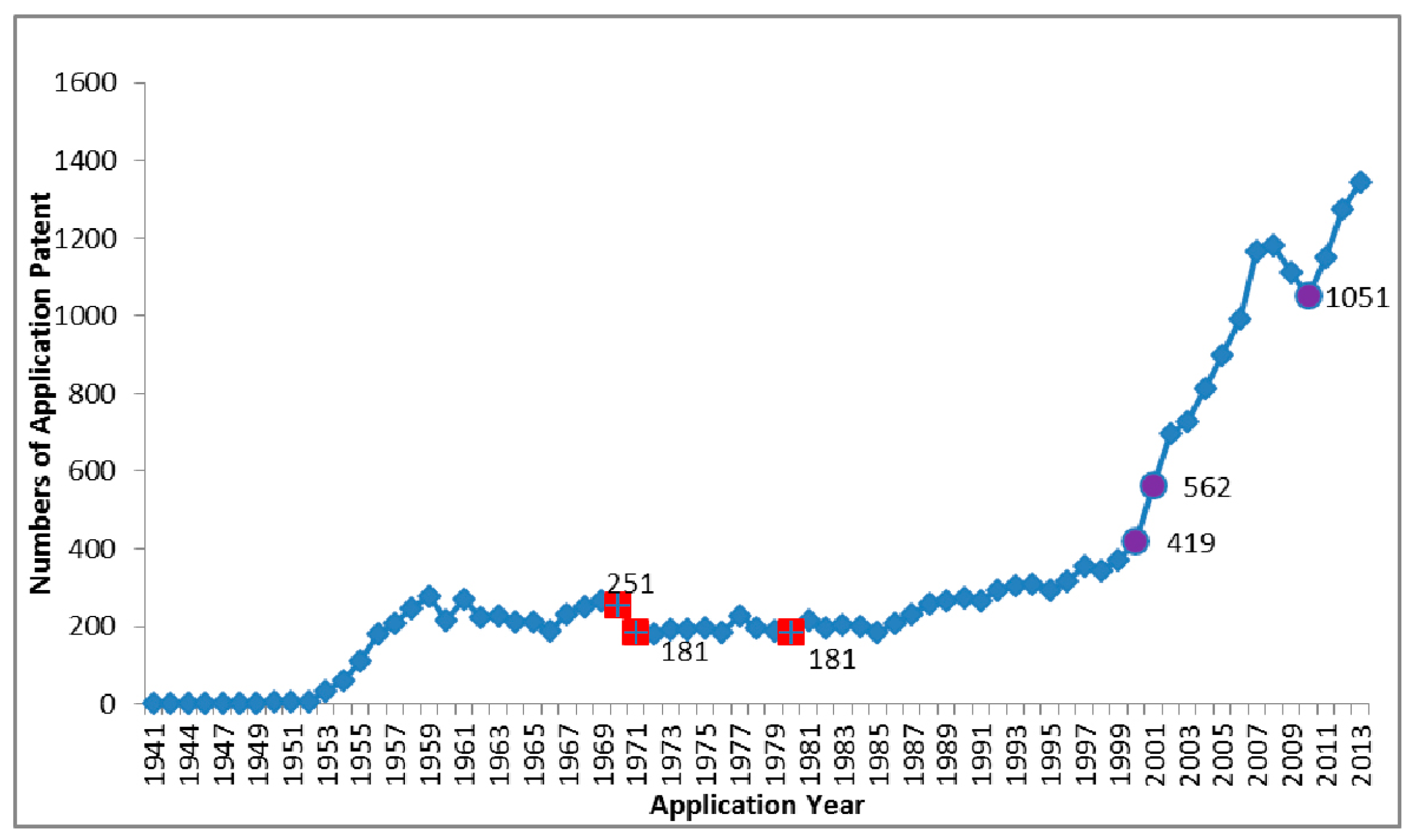
If the number of patents is accepted as a parameter of firm performance, the change of performance in the aircraft industry can be measured [19]. According to Figure 6, performance in the low knowledge society decreased in the short term from 251 in 1970 to 181 in 1971; performance also decreased in the long term of a low knowledge society, from 251 in 1970 to 181 in 1980. However, performance in the high knowledge society increased in the short term from 419 in 2000 to 562 in 2001, as well as in the long term from 419 in 2000 to 1051 in 2010. Figure 6 also shows that there is complexity in the patent performance within the aircraft industry during the past 50 years. If we look into the firm level, the complexity of performance will increase greatly.
Open innovation decreased and performance also decreased in the low knowledge society from 1970 to 1980. However, both open innovation and performance increased in the high knowledge society from 2000 to 2010. If we look into the dynamics of patents of the aircraft industry from 1941 to 2013 in Figure 6, several fluctuations are seen. Similarly, the fluctuation of open innovation from 1941 to 2013 can also be seen in Figure 4. Therefore, the complexity of the open innovation effect in the real situation of the aircraft industry can be identified according to the difference of open innovation, the difference of knowledge, and the difference in the length of time. The high knowledge society shows a greater fluctuation of performance, from 419 to 1182, compared to the low knowledge society, which ranges from its lowest value of 181 to its highest level of 251.
According to the Figure 4, Figure 5 and Figure 6, covering more than the last four decades, the open innovation effect fluctuated with different effects according to the time scope and the amounts of knowledge of the specific industry. This result is the same as the two factors from the research framework.
5. Mathematical Modeling and Simulation with the Three Factors
5.1. Mathematical Modeling of Open Innovation
Although advancing the technology of simulation in the social sciences requires appreciating its unique value as a third method of doing science in contrast to both induction and deduction, simulation can be an effective tool for discovering surprising consequences of simple assumptions [17]. There are several examples of simulation research in social science, such as a simple agent model of an epidemic, a stochastic cellular automata model of innovation diffusion, and an agent-based simulation of policy-induced diffusion of smart meters [28,29,30]. Among the simulation models, there are diverse levels such as technology adoption at the national level, knowledge transfer at the economic level, or diffusion of a residential photovoltaic system in Italy at the national level, for example [31,32,33,34]. The researchers subsequently developed a mathematical model of open innovation according to its conceptual definition at the firm level and carried out an agent-based simulation to deduce additional implications of the change of open innovation effects according to the three factors.
- T: time period for the interactions
- K(0): the amount of initial inside knowledge
- x: level of open innovation = the number of our innovators
- y: the number of other innovators
- x + y = N: the total number of innovators (constant)
- For each x, let be the performance at the time t = 0, 1, 2, …, T.
- For each x, let be the newly created performance at the time t = 0, 1, 2, …, T.
The performance outcome, , is created at the time that t1 decays as time goes by, so that at time t2, the performance becomes Γ(α, β)(t2 − t1), where Γ (α, β) (t) is the gamma function with the parameters α, β evaluated at t.
Thus, the following is obtained:
Also, assume that the initial performance is proportional to the initial amount of inside knowledge . Thus:
where δ1 is a constant.
- How can be defined?
- At each time t, innovators are categorized into three states:
- X(t): the number of our innovators who did not have interactions with other innovators
- Y(t): the number of other innovators who did not have interactions with our innovators
- I(t): the number of our innovators who are interacting with other innovators
When one of our innovators meets an outside innovator, they interact with each other. In this case, X(t) and Y(t) decrease by 1, respectively, and I(t) increases by 1. In addition, after some interaction time has passed, let this interaction time τ be separated and produce some performance output. The evolution equation for X(t), Y(t), I(t) becomes the following system of differential equations:
For all t, the following is its equality:
X(t) + Y(t) + 2I(t) = x + y = N
The discrete version for (*) is the following:
X(0) = x, Y(0) = y, I(0) = 0
Also, define by:
where δ2 is a constant.
5.2. Agent Simulation According to the Three Factors
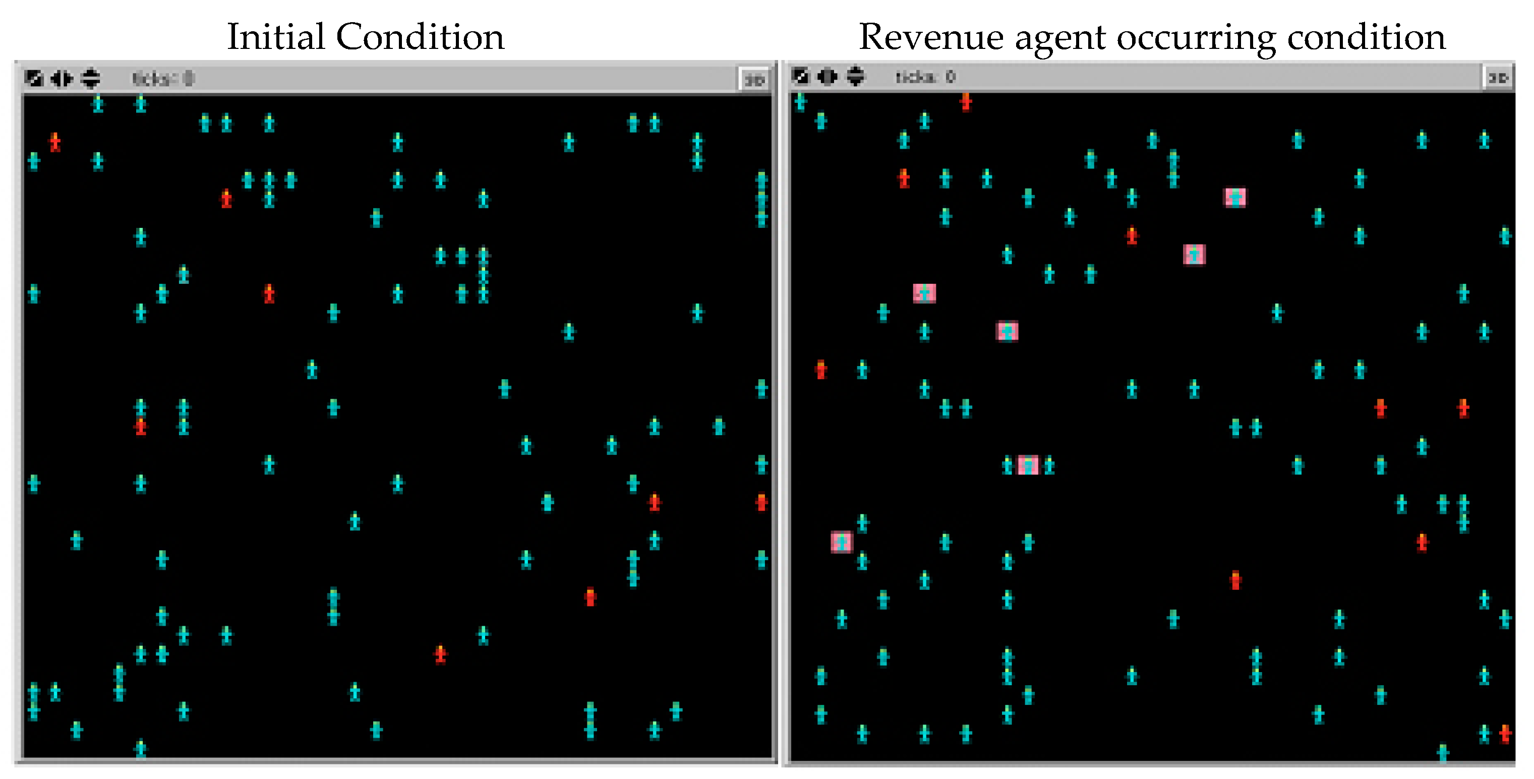
As this study simulates agents built by the mathematical model of open innovation, differentiations among agents were thus made by color: our innovator (I) is red, while the other innovator (O) is cyan (Figure 7). An interaction occurs between I and O, and I makes a random move at each tick. If I and O meet each other, an interaction occurs during a tick (10 ticks). During the interaction between I and O, performance—which is the revenue agent—occurs. The revenue agent changes according to the time and is enclosed in a square (Figure 7).
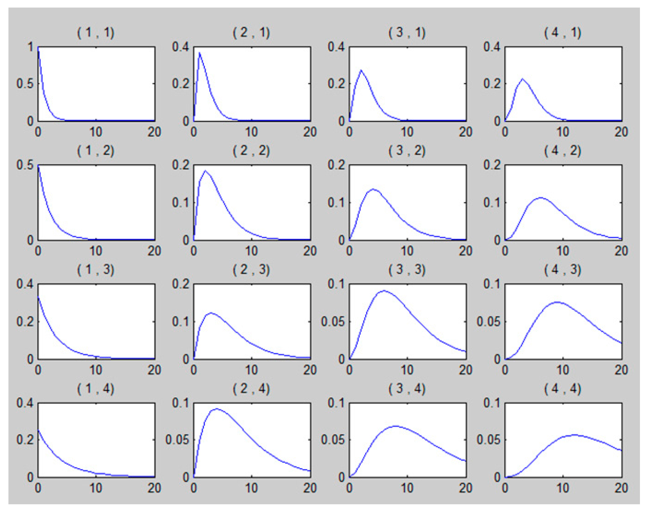
The occurring time is 𝑡_0, while the initial revenue agent is 𝑅_0. In addition, this study supposes that the revenue agent is a random variable with an average of 20, a standard deviation of 10, and that it is in a normal distribution. Also, a random sampling of revenue agents was conducted from the aforementioned supposition. The study supposed the revenue agent was an increasing coefficient according to the time, gamma curve, and a randomly selected shape/scale parameter. The shape parameter (α) was randomly selected between 1 and 4, and a 1/scale parameter (β) was also randomly selected between 1 and 4. The revenue according to time (𝑡) is (𝑡), (𝑡) = 𝑅_0 × 𝐺𝑎𝑚𝑚𝑎 (𝑡 − 𝑡_0, α, β) (Figure 8).
In simulation factors, the number of the population is the sum of the total numbers of (I) and (O). An example given in the simulation is 100 and 200.
The number of (I) among the population is 1, which is the population number.
Time span means the total time (tick number of interactions between (I) and (O)) when the number of the population and the number of (I) are decided. There are three time spans: 50, 200, and 800. Time scale 𝑘 means the change speed of revenue according to time.
K has three values: 0.5, 1, and 2.
Scale = 1: (𝑡) = 𝑅_0 × 𝐺𝑎𝑚𝑚𝑎 (𝑡 − 𝑡_0, 𝛼, 𝛽)
Scale = k: (𝑡) = 𝑅_0 × 𝐺𝑎𝑚𝑚𝑎 ((𝑡 − 𝑡_0), 𝛼, 𝛽)
An internal simulation of the mathematical model is implemented under the above conditions. First, the initial number of internal innovators of the business, which simulates the changes in open innovation performance, follows the internal knowledge amount of the business. That is, increasing the number of (I) from one to the population number simulates the changes in the revenue agent. According to Figure 9, the performance shows an inverted U-curve. In addition, with more internal initial innovators, the performance of open innovation accordingly becomes greater. Based on this simulation, it can be seen that there is high complexity from 200 performance gaps at 0 level open innovation to 20,000 performance gaps at 50–55 level open innovation. The number of internal innovators can be treated as the internal amount of knowledge.
According to Figure 10, the simulation result shows that the performance generates a bigger inverted U-curve, based on the overall number of innovators. The overall number of innovators is the total amount of knowledge. As the amount of knowledge increases, the performance boundary also increases. This means that the complexity of the open innovation performance increases as the knowledge amount increases.
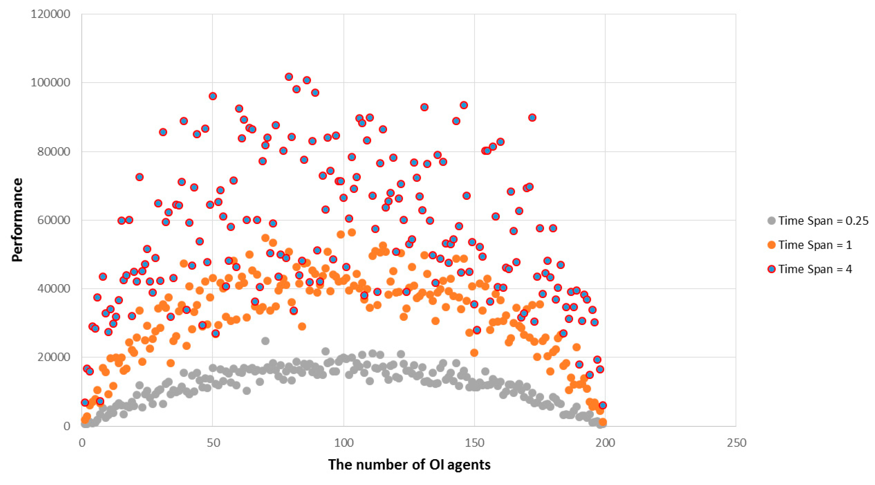
According to Figure 11, the longer the time span, the higher the inverted U-curve climbs. Thus, the open innovation performance increases to a very high level. The open innovation performance in the short-, medium-, and long-term displays an inverted U-curve, but as time is extended, the simulation results show that the open innovation performance can rise and fall to a great extent. These simulation results show that the complexity of the open innovation effect increases as the time span of the open innovation increases.
According to Figure 12, the time scale was expressed as the open innovation intensity, as the time scale corresponds to the open innovation intensity in the gamma coefficient. The simulation results show that as the intensity of open innovation increases, business performance becomes sharply augmented. For low-level open innovation, this study can also confirm that that business performance does not improve. However, as the open innovation intensity increases, complexity—which refers to the performance gaps between the highest and lowest at the same open innovation condition—also increases dramatically.
6. Logical Synthesis: Causal Loop Modeling of the Open Innovation Effect with the Three Factors
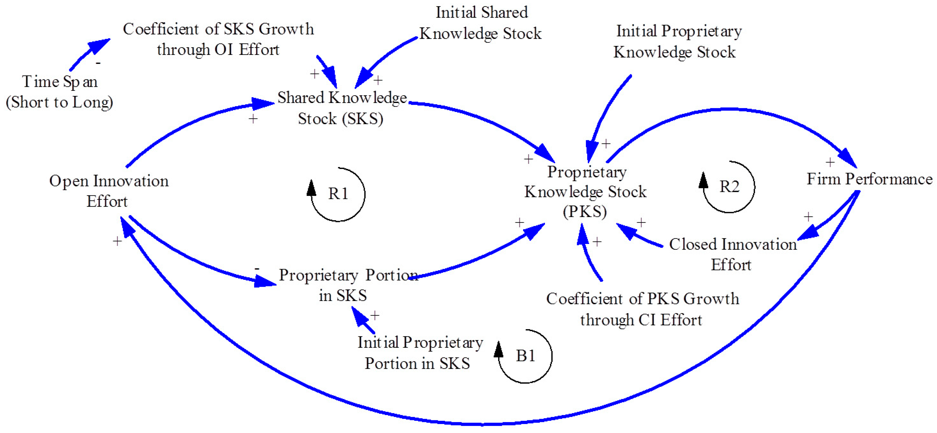
By discussing the important variables of the causal model, two types of innovation effort (or innovation investment) can be considered: the open innovation effort, which creates shared knowledge stock (SKS), and the closed innovation effort, which creates a proprietary knowledge stock (PKS). In addition, two types of knowledge stock, SKS and PKS, exist. A portion of SKS can be converted into PKS. Firm performance (or profit) can come from PKS and SKS. There are two coefficients of knowledge stock (KS). SKS is a coefficient of SKS growth through OI. PKS is a coefficient of PKS growth through CI; two coefficients of KS increase efficiency through the innovation effort. A coefficient of SKS grows through open innovation (CoSKSGr_OI) and is assumed to decrease over time; as such, maturation will occur. A coefficient of PKS grows through CI (CoPKSGr_CI), which is assumed to remain unchanged. In a future study, the case where the coefficient of PKS growth through CI also decreases over time or with PKS maturation (the Maturation Effect of PKS Building through CI) can be studied. There are three preconditions or initial knowledge stocks: initial SKS, initial PKS, and the initial proprietary portion in SKS. This study accepts the effect of time span from the short term to the long term.
“Time Span” ↑ → “Coefficient of SKS Growth through OI” ↓
The causal loop in Figure 13 shows that balance between positive and negative effects of the open innovation effort, as well as the reinforcing effect of the CI effort and the basic loop related to the open innovation effort—as shown in Table 2—exist. While open innovation effects have statistically been the cause of the inverted U-curve through the action of the balancing loop B1 and the reinforcement loops R1 and R2, extremely diversified forms of open innovation effects continue to appear. A better understanding of these logical developments can be gained through an intuitive grasp of the data shown in Table 2.
If the argument for “effect of Time Span (Short, Long)”—that is, the maturation effect of the OI effort—unfolds, a better explanation for this causal loop can be given. Assuming that the “coefficient of SKS growth through open innovation (OI)” goes down as time passes by (Short → Long), a maturation effect occurs: Time Span ↑ → Coefficient of SKS Growth through OI ↓ → Shared Knowledge Stock (SKS) ↓ → Proprietary Knowledge Stock (PKS) ↓ → Firm Performance ↓ → OI Effort ↓. Therefore, if it is also assumed that the “Coefficient of PKS Growth through CI” remains unchanged, it will be more profitable to “focus on the CI effort rather than the OI effort in a later stage.” As a result, “in the earlier stage → the focus is on OI” and “in the later stage → the focus is on CI”.
The “effect of Initial Knowledge Stock” will be discussed next. If the “initial PKS” is high enough and the “coefficient of PKS growth through CI” also remains high enough, then more focus can be given to R2 (CI) rather than R1 (OI), because R2 (CI) can independently provide enough efficiency in PKS building. However, focus must be given to open innovation rather than CI with a low “initial PKS” and a low “coefficient of PKS growth through CI”.
In addition, with a high “initial proprietary portion in SKS”, it may be somewhat harmful to use open innovation because it will significantly lower the “proprietary portion in SKS”, thus also reducing PKS and firm performance. This effect will be more severe when the OI maturation effect occurs. Earning is not possible from open innovation because the SKS is already matured, and the “proprietary portion in SKS” will only be lost. When the shared knowledge stock (SKS) is too small and the “coefficient of SKS growth through open innovation” is also small, using open innovation will not be helpful at all; in this case, the focus must be on CI rather than open innovation.
Finally, the short- and long-term effects that open innovation efforts exert on business performance in the relationship with R1, R2, and B1 are important factors that decide the content structure and the direction of the performance. In the early stages, open innovation effects rode on the open innovation reinforcement loop of R1 and acted more strongly than the balanced loop B1, thus providing a positive impact on the business performance. However, if open innovation efforts become bigger, the close innovation effects of R2 will gradually become bigger than the open innovation effects. Furthermore, as B1 has also grown bigger, the business performance stops growing and, sometimes, may even deteriorate.
Through the logic model of the causal loop in Figure 13, the reinforcement loops R1 and R2, including the balanced loop B1, each have a mutual interaction with the effect of the time span, the effect of the initial knowledge stock, and the open innovation effort. Many fluctuations and complexities occur through the mutual interaction among the reinforcement loops R1 and R2 and the balanced loop B1 according to the situations of time span, the effect of the initial knowledge stock, and the open innovation effort. Looking at the general inverted U-curve, the point that connects business performance in various forms can be concretely and logically understood using the complex inverted U-curve open innovation effect causal loop model with three major factors.
According to Figure 13, open innovations with different open innovation strategies, different industry conditions, and different time scopes eventually have positive feedback loops, and balancing feedback loops at the same time. This causal loop means that open innovation effects can be the inverted U-curve, the fluctuated, and diverse at the same time.
7. Discussion
According to the results of the four research methods, we find out that the dynamics of open innovation is not just an inverted U-curve but also fluctuated, and diverse, according to several factors including the open innovation strategy, the specific industry, and the time scope for analysis.
If firms augment open innovation, will the business performance inevitably increase? The answer is no. Should the open innovation of firms be augmented, open innovation might increase the business performance to a certain level, after which the business performance would start to follow the decreasing inverted U-curve [9,11,35]. However, depending on the specific size of the firm existing in various time dimensions, the industry where the firm belongs (i.e., the open innovation characteristics of the corresponding industry or the open innovation intensity), and on the time dimension where the corresponding open innovation is in progress, open innovation can create various levels of performance. Therefore, it cannot simply be concluded that through an initial augmentation of open innovation and a later reinforcement of closed innovation, firms can improve business performance. The most certain and quickest way to fall into an innovator’s dilemma is by understanding the relationships between open innovation and business performance as a simple inverted U-curve [36]. Furthermore, open innovation affects economic dynamics on a more macroscopic level: not only through the relationship between open innovation and closed innovation, but also through the dynamics of open innovation and social innovation [37]. In other words, through several feedback loops, such as the open innovation of a knowledge city and the open innovation of a national innovation system, powerful open innovation reinforcement loops exist on the macro level [38]. Also, the development and application of various business models that connect the firms and the market together with open innovation have to be newly understood and explained through a reinforcement of open innovation or balanced loops [39].
From the game of life, mathematical model–based simulations, field research about aircraft industries, and causal loop building, the complex inverted U-curve open innovation effect model with three major factors can be understood from diverse aspects. Open innovation creates an inverted U-curve performance with a high-level fluctuation complexity according to three major factors: knowledge intensity, open innovation strategy, and time span. In addition, if we bear in mind the competitors that firms have, the complexity of open innovation effects will dramatically increase [40].
8. Conclusions
Open innovation is a paradigm which assumes that companies can and should use external ideas as well as internal ideas, and internal and external paths to market, as the companies look to advance their technology [41]. This study on open innovation revealed several pieces of evidence about the various complex relationships between open innovation and business performance, from a game of life simulation, mathematical modeling and simulation, an aircraft industry patent analysis, and causal loop modeling.
The three different open innovation effect models and the one real industry analysis show the concrete context of the equivocal and complex aspects of the relationship between open innovation and business performance. One important conclusion of this research is that the impact of open innovation on business performance is very dynamic and appears in unpredictable forms.
The value of the results of this study from simulations in various dimensions cannot be ignored. However, future research is required to develop a systematic analysis that will explain and present the form or appearance under which open innovation activities specifically influence business performance from the aspects of specific time spans, open innovation conditions, and knowledge or technology accumulation with diverse competitors.
Acknowledgments
This work was supported by the DGIST R&D Program of the Ministry of Science, ICT and Future Planning (16 and 17). This paper was first presented at the Society of Open Innovation: Technology, Market, and Complexity (SOItmC) 2016 with the title “Open the Black Box of the Open Innovation effect: by game of life simulation about the reverse U-curve”, and was fully developed based on comments received from anonymous reviewers during the conference. The revised paper was presented at the following SOItmC 2017 with the title of “Dismantling of the Inverted U-curve”. The current version has been fully developed based on comments from anonymous reviewers during the last conference. We thank anonymous reviewers of the journal that helped us improve the paper.
Author Contributions
This paper represents a result of teamwork. JinHyo Joseph Yun designed the research and wrote the full draft of the paper; DongKyu Won conducted the game of life simulation; EuiSeob Jeong conducted patent data mining of the aero industry; KyungBae Park built the causal loop model; DooSeok Lee conducted the mathematical modeling; and Tan Yigitcanlar finalized the manuscript. All authors read and approved the final paper.
Conflicts of Interest
The authors declare no conflict of interest.
References
- Sabatini-Marques, J.; Yigitcanlar, T.; Da Costa, E. Australian innovation ecosystem. Asia Pac. J. Innov. Entrep. 2015, 9, 3–28. [Google Scholar]
- Sabatini-Marques, J.; Yigitcanlar, T.; Da Costa, E. Incentivizing innovation. Asia Pac. J. Innov. Entrep. 2015, 9, 31–56. [Google Scholar]
- Yigitcanlar, T.; Sabatini-Marques, J.; Da Costa, E.; Kamruzzaman, M.; Ioppolo, G. Stimulating technological innovation through incentives. Technol. Forecast. Soc. Chang. 2017, in press. [Google Scholar] [CrossRef]
- Barge-Gil, A. Open, semi-open and closed innovators: Towards an explanation of degree of openness. Ind. Innov. 2010, 17, 577–607. [Google Scholar] [CrossRef]
- Drechsler, W.; Natter, M. Understanding a firm’s openness decisions in innovation. J. Bus. Res. 2012, 65, 438–445. [Google Scholar] [CrossRef]
- Laursen, K.; Salter, A. Open for innovation: The role of openness in explaining innovation performance among U.K. manufacturing firms. Strateg. Manag. J. 2006, 27, 131–150. [Google Scholar] [CrossRef]
- Porter, M.E. Competitive Advantage: Creating and Sustaining Superior Performance; Free Press: New York, NY, USA, 1985; pp. 235–237. ISBN 0684841460. [Google Scholar]
- Van de Vrande, V.; de Jong, J.P.; Vanhaverbeke, W.; de Rochemont, M. Open innovation in SMEs: Trends, motives and management challenges. Technovation 2009, 29, 423–437. [Google Scholar] [CrossRef]
- Yun, J.H.J. How do we conquer the growth limits of capitalism? J. Open Innov. Technol. Market Complex. 2015, 1, 1–20. [Google Scholar]
- Yun, J.J.; Jeong, E.; Yang, J. Open innovation of knowledge cities. J. Open Innov. Technol. Market Complex. 2015, 1, 1–20. [Google Scholar] [CrossRef]
- Yun, J.J.; Won, D.; Hwang, B.; Kang, J.; Kim, D. Analysing and simulating the effects of open innovation policies: Application of the results to Cambodia. Sci. Public Policy 2015, 42, 743–760. [Google Scholar] [CrossRef]
- Theyel, N. Extending open innovation throughout the value chain by small and medium-sized manufacturers. Int. Small Bus. J. 2012, 31, 256–274. [Google Scholar] [CrossRef]
- Parida, V.; Westerberg, M.; Frishammar, J. Inbound open innovation activities in high-tech SMEs: The impact on innovation performance. J. Small Bus. Manag. 2012, 50, 283–309. [Google Scholar] [CrossRef]
- Lee, S.; Park, G.; Yoon, B.; Park, J. Open innovation in SMEs: An intermediated network model. Res. Policy 2010, 39, 290–300. [Google Scholar] [CrossRef]
- West, J.; Bogers, M. Leveraging external sources of innovation: A review of research on open innovation. J. Prod. Innov. Manag. 2014, 31, 814–831. [Google Scholar] [CrossRef]
- Jeon, J.H.; Kim, S.L.; Koh, J.H. Historical review on the patterns of open innovation at the national level: The case of the Roman period. J. Open Innov. Technol. Market Complex. 2015, 1, 1–17. [Google Scholar] [CrossRef]
- Patra, S.K.; Krishna, V.V. Globalization of R&D and open innovation: Linkages of foreign R&D centers in India. J. Open Innov. Technol. Market Complex. 2015, 1, 1–24. [Google Scholar]
- Kodama, F.; Shibata, T. Demand articulation in the open-innovation paradigm. J. Open Innov. Technol. Market Complex. 2015, 1, 1–21. [Google Scholar] [CrossRef]
- Bhargava, S.C.; Kumar, A.; Mukherjee, A. A stochastic cellular automata model of innovation diffusion. Technol. Forecast. Soc. Chang. 1993, 44, 87–97. [Google Scholar] [CrossRef]
- Schulman, L.S.; Seiden, P.E. Statistical mechanics of a dynamical system based on conway’s game of life. J. Stat. Phys. 1978, 19, 293–314. [Google Scholar] [CrossRef]
- Brunswicker, S.; Vanhaverbeke, W. Beyond Open Innovation in Large Enterprises: How do Small and Medium-Sized Enterprises (SMEs) Open up to External Innovation Sources? SSRN [Online], 2011. Available online: https://ssrn.com/abstract=1925185 (accessed on 4 August 2017). [CrossRef]
- Bays, C. A new candidate rule for the game of three-dimensional life. Complex Syst. 1992, 6, 433–441. [Google Scholar]
- Blok, H.J.; Bergersen, B. Effect of boundary conditions on scaling in the “game of Life”. Phys. Rev. E 1997, 55, 6249. [Google Scholar] [CrossRef]
- Rennard, J.P. Implementation of Logical Functions in the Game of Life. In Collision-Based Computing; Adamatzky, A., Ed.; Springer: London, UK, 2002; pp. 491–512. ISBN 978-1-4471-0129-1. [Google Scholar]
- Axelrod, R. Advancing the Art of Simulation in the Social Sciences. In Simulating Social Phenomena; Conte, R., Hegselmann, R., Terna, P., Eds.; Springer: Berlin, Germany, 1997; pp. 21–40. ISBN 978-3-540-63329-7. [Google Scholar]
- Björk, S.; Juul, J. Zero-Player Games or: What We Talk About when We Talk About Players. In Proceedings of the Philosophy of Computer Games Conference, Madrid, Spain, 29–31 January 2012. [Google Scholar]
- Yun, J.J.; Won, D.; Park, K. Dynamics from open innovation to evolutionary change. J. Open Innov. Technol. Market Complex. 2016, 2, 1–22. [Google Scholar] [CrossRef]
- Yun, J.J.; Jeong, E.; Park, J. Network Analysis of Open Innovation. Sustainability 2016, 8, 729. [Google Scholar] [CrossRef]
- Gordon, T.J. A simple agent model of an epidemic. Technol. Forecast. Soc. 2003, 70, 397–417. [Google Scholar] [CrossRef]
- Rixen, M.; Weigand, J. Agent-based simulation of policy induced diffusion of smart meters. Technol. Forecast. Soc. Chang. 2014, 85, 153–167. [Google Scholar] [CrossRef]
- März, S.; Friedrich-Nishio, M.; Grupp, H. Knowledge transfer in an innovation simulation model. Technol. Forecast. Soc. Chang. 2006, 73, 138–152. [Google Scholar] [CrossRef]
- Palmer, J.; Sorda, G.; Madlener, R. Modeling the diffusion of residential photovoltaic systems in Italy: An agent-based simulation. Technol. Forecast. Soc. Chang. 2015, 99, 106–131. [Google Scholar] [CrossRef]
- Swinerd, C.; McNaught, K.R. Comparing a simulation model with various analytic models of the international diffusion of consumer technology. Technol. Forecast. Soc. Chang. 2015, 100, 330–343. [Google Scholar] [CrossRef]
- Christensen, C.M. The Innovator’s Dilemma: When New Technologies Cause Great Firms to Fail; Harvard Business School Press: Boston, MA, USA, 1997; p. 14. [Google Scholar]
- Yun, J.H.J.; Won, D.K.; Jeong, E.S.; Park, K.B.; Yang, J.H.; Park, J.Y. The relationship between technology, Business Model, and market in autonomous car and intelligent robot industries. Technol. Forecast. Soc. Chang. 2016, 103, 142–155. [Google Scholar] [CrossRef]
- Deeds, D.L.; Hill, C.W. Strategic alliances and the rate of new product development: An empirical study of entrepreneurial biotechnology firms. J. Bus. Ventur. 1996, 11, 41–55. [Google Scholar] [CrossRef]
- Greco, M.; Grimaldi, L.; Cricelli, L. Open innovation actions and innovation performance: A literature review of European empirical evidence. Eur. J. Innov. Manag. 2015, 18, 150–171. [Google Scholar] [CrossRef]
- Bayona-Saez, C.; Cruz-Cázares, C.; García-Marco, T.; Sánchez García, M. Open innovation in the food and beverage industry. Manag. Decis. 2017, 55, 526–546. [Google Scholar] [CrossRef]
- Yun, J.; Lee, D.; Ahn, H.; Park, K.; Lee, S.; Yigitcanlar, T. Not deep learning but autonomous learning of open innovation for sustainable artificial intelligence. Sustainability 2016, 8, 797. [Google Scholar] [CrossRef]
- Yun, J.; Yigitcanlar, T. Open innovation in value chain for sustainability of firms. Sustainability 2017, 9, 811. [Google Scholar] [CrossRef]
- Chesbrough, H.W. Open Innovation: The New Imperative for Creating and Profiting from Technology; Harvard Business Press: Boston, MA, USA, 2006. [Google Scholar]
Figure 1.
Research framework on open innovation effects according to three factors.

Figure 2.
Simulation results in low knowledge condition.

Figure 3.
Simulation results in high knowledge condition.

Figure 4.
Open innovation trends in the aircraft industry by year.

Figure 5.
Comparison between the 1970s and 2000s in the open innovation of the aircraft industry.

Figure 6.
Trends of the total patents by year.

Figure 7.
Agent-based simulation. Revenue agent = (𝑡; 𝛽).

Figure 8.
Revenue change by gamma curves. Revenue agent = Gamma (𝑡; α, β) with the shape parameter α and the 1/scale parameter β.
Figure 8.
Revenue change by gamma curves. Revenue agent = Gamma (𝑡; α, β) with the shape parameter α and the 1/scale parameter β.

Figure 9.
Performance change according to internal innovators.

Figure 10.
Performance changes according to the total number of innovators.

Figure 11.
Performance changes according to the time span.

Figure 12.
Performance changes according to open innovation intensity.

Figure 13.
Causal model of open innovation effort, knowledge stock, and firm.


Table 1.
Game of life simulation according to the three factors.
| A (LSS) | B (LSL) | E(LBS) | F(LBL) |
| OI Low | OI Low | OI Low | OI Low |
| K Small | K Small | K Big | K BIG |
| T Short | T Long | T Short | T Long |
| C(HSS) | D(HSL) | G(HBS) | H(HBL) |
| OI High | OI High | OI High | OI High |
| K Small | K Small | K Big | K Big |
| T Short | T Long | T Short | T Long |
Table 2.
Major feedback loops.
| (R1, Basic Loop, OI Effort) Reinforcing Effect of OI Effort |
| OI Effort ↑ → Shared Knowledge Stock (SKS) ↑ → Proprietary Knowledge Stock (PKS) ↑ → Firm Performance ↑ → OI Investment ↑ |
| (R2, CI Effort) Reinforcing Effect of CI Effort |
| CI Effort ↑ → Proprietary Knowledge Stock (PKS) ↑→ Firm Performance ↑ → CI Effort ↑ |
| (B1, Negative Effect of OI Effort) Balancing Effect of OI Effort |
| OI Effort ↑ → Proprietary Portion in SKS ↓ → Proprietary Knowledge Stock (PKS) ↓ → Firm Performance ↓ → OI Effort ↓ |
© 2017 by the authors. Licensee MDPI, Basel, Switzerland. This article is an open access article distributed under the terms and conditions of the Creative Commons Attribution (CC BY) license (http://creativecommons.org/licenses/by/4.0/).
Share and Cite
MDPI and ACS Style
Yun, J.J.; Won, D.; Jeong, E.; Park, K.; Lee, D.; Yigitcanlar, T. Dismantling of the Inverted U-Curve of Open Innovation. Sustainability 2017, 9, 1423. https://0-doi-org.brum.beds.ac.uk/10.3390/su9081423
AMA Style
Yun JJ, Won D, Jeong E, Park K, Lee D, Yigitcanlar T. Dismantling of the Inverted U-Curve of Open Innovation. Sustainability. 2017; 9(8):1423. https://0-doi-org.brum.beds.ac.uk/10.3390/su9081423
Chicago/Turabian StyleYun, JinHyo Joseph, DongKyu Won, EuiSeob Jeong, KyungBae Park, DooSeok Lee, and Tan Yigitcanlar. 2017. "Dismantling of the Inverted U-Curve of Open Innovation" Sustainability 9, no. 8: 1423. https://0-doi-org.brum.beds.ac.uk/10.3390/su9081423
Note that from the first issue of 2016, this journal uses article numbers instead of page numbers. See further details here.