Article

Polarimetric Emission of Rain Events: Simulation and Experimental Results at X-Band

Dept. of Signal Theory and Communications, Universitat Politècnica de Catalunya, UPC Campus Nord D3, E-08034 Barcelona, Spain, and SMOS Barcelona Expert Centre, Pg. Marítim de la Barceloneta 37-49, E-08003, Barcelona, Spain
*
Author to whom correspondence should be addressed.
Remote Sens. 2009, 1(2), 107-121; https://0-doi-org.brum.beds.ac.uk/10.3390/rs1020107
Submission received: 4 May 2009 / Revised: 5 June 2009 / Accepted: 9 June 2009 / Published: 12 June 2009
(This article belongs to the Special Issue Microwave Remote Sensing)

Abstract

:
Accurate models are used today for infrared and microwave satellite radiance simulations of the first two Stokes elements in the physical retrieval, data assimilation etc. of surface and atmospheric parameters. Although in the past a number of theoretical and experimental works have studied the polarimetric emission of some natural surfaces, specially the sea surface roughened by the wind (Windsat mission), very limited studies have been conducted on the polarimetric emission of rain cells or other natural surfaces. In this work, the polarimetric emission (four Stokes elements) of a rain cell is computed using the polarimetric radiative transfer equation assuming that raindrops are described by Pruppacher-Pitter shapes and that their size distribution follows the Laws-Parsons law. The Boundary Element Method (BEM) is used to compute the exact bistatic scattering coefficients for each raindrop shape and different canting angles. Numerical results are compared to the Rayleigh or Mie scattering coefficients, and to Oguchi’s ones, showing that above 1-2 mm raindrop size the exact formulation is required to model properly the scattering. Simulation results using BEM are then compared to the experimental data gathered with a X-band polarimetric radiometer. It is found that the depolarization of the radiation caused by the scattering of non-spherical raindrops induces a non-zero third Stokes parameter, and the differential phase of the scattering coefficients induces a non-zero fourth Stokes parameter.

1. Introduction: Theoretical Formulation of the Polarimetric Emission by Rain

Accurate models are used today for infrared and microwave satellite radiance simulations of the first two Stokes elements in the physical retrieval, data assimilation etc. of surface and atmospheric parameters [1]. Although in the past a number of theoretical and experimental works have studied the polarimetric emission of some natural surfaces, specially the sea surface roughened by the wind (Windsat mission) [2], very limited studies have been conducted on the polarimetric emission of rain cells or other natural surfaces [3,4,5,6].
Emission models at vertical and horizontal polarizations originated by rain cells have been intensively studied (see for example the intercomparison performed in [7]), but very few studies have been conducted to study the full polarimetric emission of rain cells [3,4,5].
The polarimetric emission of a rain cell can be computed by means of the Radiative Transfer Equation (RTE) [6]:
cos θ d T ¯ B ( θ , ϕ , z ) d z = k = e ( θ , ϕ ) T ¯ B ( θ , ϕ , z ) + F ¯ ( θ , ϕ ) ( T , z ) + 0 2 π   0 π P = ( θ , ϕ , θ , ϕ ) T ¯ B ( θ , ϕ , z )   d
where T ( z ) is the temperature distribution, the Stokes vector T ¯ B is related to the electric fields incident in the antenna at vertical and horizontal polarizations (Ev and Eh [V/m]) by [8]:
[ T v ( θ , ϕ ) T h ( θ , ϕ ) T U ( θ , ϕ ) T V ( θ , ϕ ) ] = λ 2 η k B B [ E v E v * E h E h * 2 Re E v E h * 2 Im E v E h * ]
and:
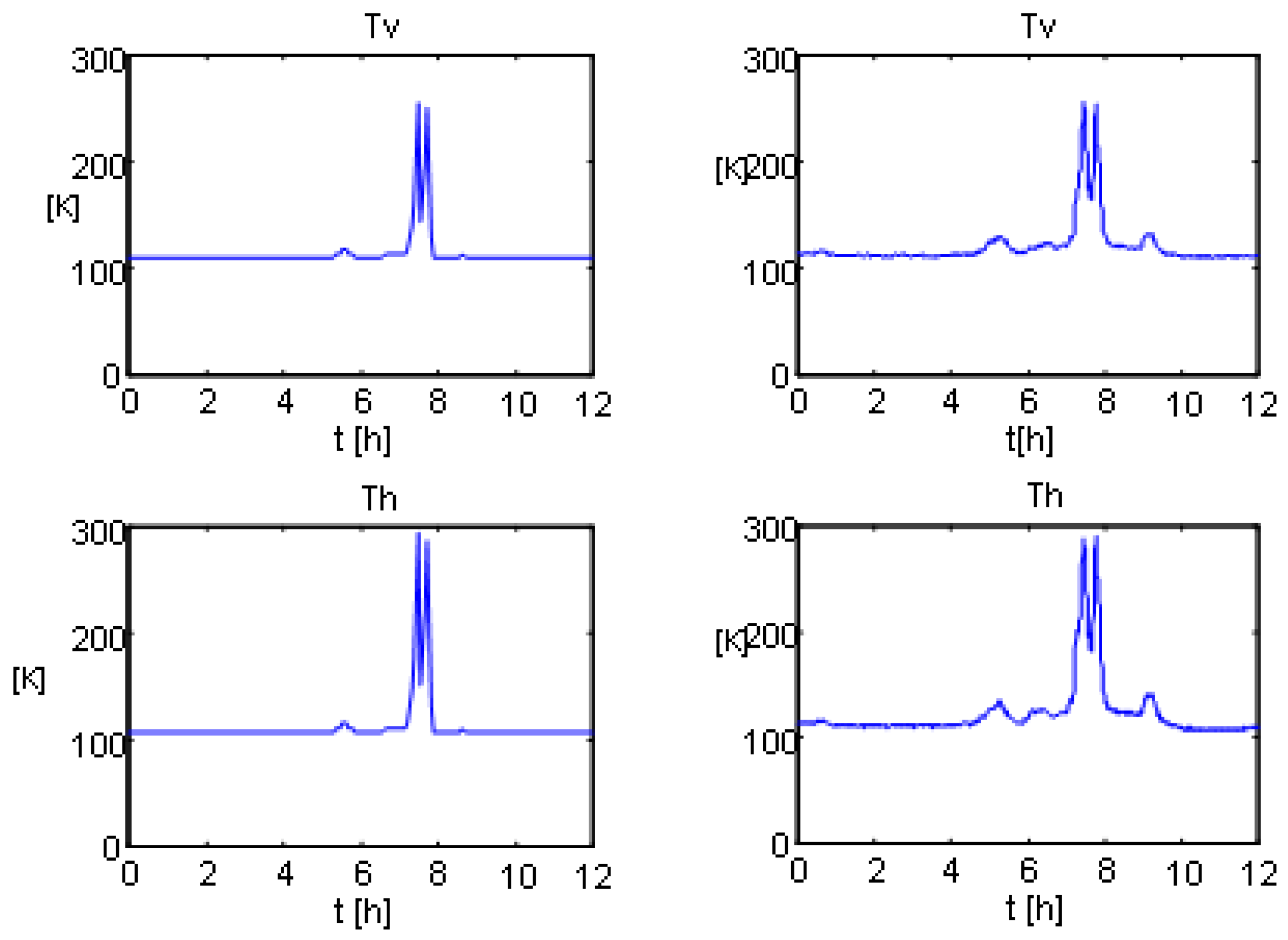
  • Tv and Th are brightness temperatures at vertical and horizontal polarizations, respectively (Instead of Tv and Th, the first and second Stokes parameters are sometimes defined as I = Tv + Th, and Q = Tv-Th),
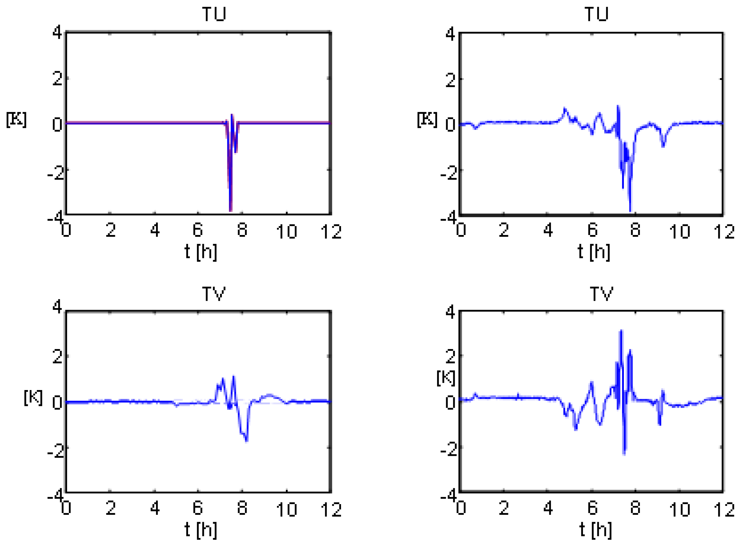
  • TU and TV are the third and fourth Stokes elements, respectively,
  • λ is the electromagnetic wavelength, η is the wave impedance, kB is the Boltzmann’s constant, and B is the radiometer’s bandwidth.
The extinction matrix k = e in (1) is given by:
k = e = 2 π n 0 k [ 2 S m f v v 0 S m f v h R e f v h 0 2 S m f h h S m f h v R e f h v 2 S m f h v 2 S m f v h S m f v v + f h h R e f v v f h h 2 R e f h v 2 R e f v h R e f h h f v v S m f v v + f h h ] ,
where n0 is the number of particles per unit of volume, k is the wave number, fpq are the forward scattering amplitudes, and the operator < > stands for the average over the ensemble of scatterers in the volume (raindrops, each one with a canting angle).
The emission vector F ¯ is given by:
F ¯ ( θ , ϕ ) = [ k a 1 ( π θ , π + ϕ ) k a 2 ( π θ , π + ϕ ) k a 3 ( π θ , π + ϕ ) k a 4 ( π θ , π + ϕ ) ] T , k a 1 ( θ , ϕ ) = k e 11 ( θ , ϕ ) 0 2 π 0 π [ P 11 ( θ , φ , θ , φ ) + P 21 ( θ , φ , θ , φ ) ] d Ω , k a 2 ( θ , ϕ ) = k e 22 ( θ , ϕ ) 0 2 π 0 π [ P 12 ( θ , φ , θ , φ ) + P 22 ( θ , φ , θ , φ ) ] d Ω , k a 3 ( θ , ϕ ) = 2 k e 13 ( θ , ϕ ) + 2 k e 23 ( θ , ϕ ) 2 0 2 π 0 π [ P 13 ( θ , φ , θ , φ ) + P 23 ( θ , φ , θ , φ ) ] d Ω , k a 4 ( θ , ϕ ) = 2 k e 14 ( θ , ϕ ) 2 k e 24 ( θ , ϕ ) + 2 0 2 π 0 π [ P 14 ( θ , φ , θ , φ ) + P 24 ( θ , φ , θ , φ ) ] d Ω .
and the phase matrix P = is given by:
P = ( θ , θ , ϕ , ϕ ) = n 0 [ | f w | 2 | f v h | 2 R e f w f v h * S m f v v f v h * | f h v | 2 | f h h | 2 R e f h v f h h * S m f h v f h h * 2 R e f w f h v * 2 R e f v h f h h * R e f v v f h h * + f v h f h v * S m f v v f h h * + f v h f h v * 2 S m f v v f h v * 2 S m f v h f h h * S m f v v f h h * + f v h f h v * R e f v v f h h * + f v h f h v * ] .
In Equation (5) the fpq coefficients are the vector-scattering amplitude functions that provide the amplitude, phase and polarization information of the scattered field at q-polarization E q = e q f p q ( θ , θ , ϕ , ϕ ) e j k r / r , when a plane wave at p-polarization E i = e q e j K i n r r is incident on each scatterer, and as in Equation (3) the operator < > stands for the average over the ensemble of scatterers in the volume.
The solution of Equation (1) entails the application of the following boundary conditions: T ¯ B ( θ , ϕ , z = 0 ) at the Earth’s surface, and T ¯ B ( θ , ϕ , z = h ) = [ 0   0   0   0 ] T on top of the atmosphere. This condition means that external radiations (cosmic and galactic noise) are negligible in front of the radiation introduced by the rain cell itself.
Section 2 describes the formulation of the computation of the fpq scattering coefficients using the Boundary Elements Method (BEM). Numerical results are presented and compared with previously reported values and Rayleigh and Mie scattering coefficients. Section 3 presents experimental data gathered with an X-band fully-polarimetric radiometer and compares it with the numerical predictions performed using the polarimetric RTE and the BEM. Finally, Section 4 summarizes the main conclusions.

2. Computation of the Scattering by Raindrops Using the Boundary Element Method

The scattering properties of spherical hydrometeors can be computed using [9]:
  • the Rayleigh approximation for small spheres in comparison with wavelength,
  • the Mie expression for spheres whose size is comparable to wavelength, or
  • optical approximation for spheres much larger than the wavelength.
In practice, many hydrometeors are not spherical, but their shape can often be approximated by an ellipsoid or spheroid. Figure 1a shows the raindrop shapes for 13 different equivalent radii from 0.25 to 3.25 mm [10]. As it can be appreciated, the larger the equivolumetric raindrop radius, due to air friction, the larger the shape distorsion from the spherical shape (This process is more complex since raindrops merge and break, and their shape oscillates around the equilibrium shape). Recent measurements of drop shapes by video disdrometer under calm air conditions seem to show that the Pruppacher-Pitter model slightly overestimates the real drop deformation [11,12,13] although the contribution of large drops to the total EM scattering properties is relatively small because of their small number density. Figure 1b shows the Laws-Parsons equivalent radii distribution as a function of the rain rate [14].
Figure 1a. Shape of a raindrop for equivalent radii: 0.25, 0.50 … 3.25 mm.
Remotesensing 01 00107 g001a
Figure 1b. Laws and Parsons equivalent radii distribution vs. rain rate (0.25 … 150 mm/h).
Remotesensing 01 00107 g001b
If the ellipsoid size is small compared with a wavelength, a Rayleigh static solution can be used. For spheroidal obstacles the spheroidal function expansion method seems to be a good approximation [15]. However, for large drops the shape is not that simple and it is necessary to apply a numerical method to determine the scattering coefficients fpq. A number of different methods has been developed: point-matching, T-matrix, unimoment, and Fredholm Integral Equation [16,17].
In this paper the Boundary Element Method (BEM) [18] is applied to compute the electromagnetic fields inside and outside dielectric scatterers. The advantage in the Boundary Element Method (BEM) arises from the fact that only the boundary of the domain of the integral equation requires meshing. Thus, the dimension of the problem is effectively reduced by one, that is, the integral equation governing a three dimensional region is transformed into one over its surface. The discretization of only dielectric surfaces reduces user input and storage requirements. The method not only produces precise results with far less data as compared to the methods of finite differences and finite elements, but also works with open region problems without any truncation of the region. The fact that the elements have a parabolic shape makes that BEM models solve problem geometries accurately.

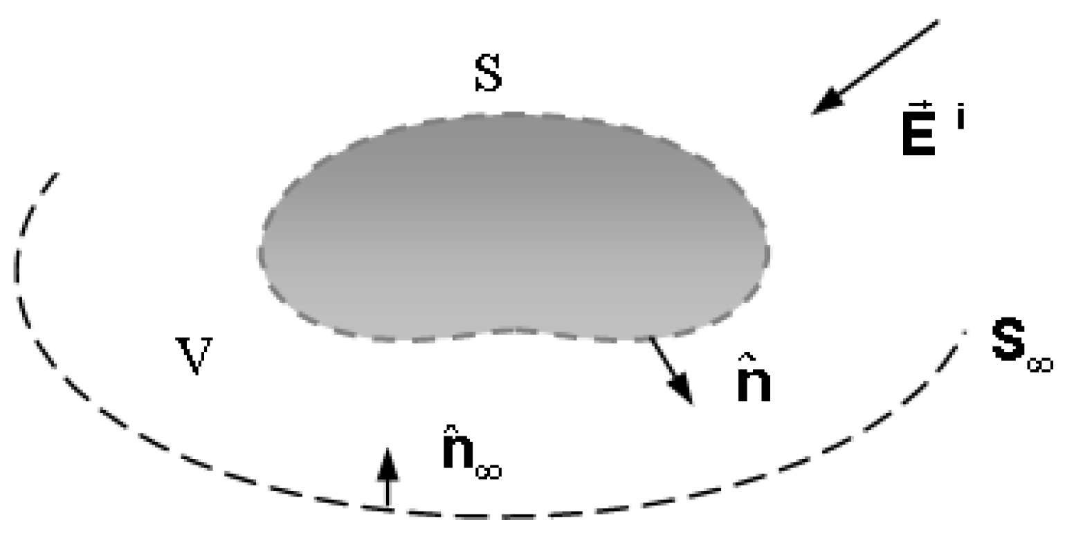
2.1. Formulation of the Boundary Element Method (BEM)

In the BEM the scattering problem is formulated in terms of a surface integral equation. The region V is source-free and it is filled with a homogeneous material bounded by a surface S (Figure 2a). The surface S is divided into curvilinear elements. Assuming a time dependence of the electromagnetic fields as exp ( j ω t ) , the integral equation for node ‘i’ located at r on S is given by [18]:
α i H i = S { j ω ε ( n ^ × E ) G i + ( n ^ × H ) × G i + ( n ^ H ) G i } d S ,
where:
α i = V δ ( r r ) d V ,
ε is the dielectric permittivity, Gi is the free space Green’s function, and R = | r r | is the distance between the field point and the source point on the surface.
The surface is discretized using the Finite Element Method with second order isoparametric elements and the electromagnetic fields on each element are approximated using the same weighting functions as for the surface’s discretization.
Applying Equation (6) to each node ‘i’ successively, a system of equations is obtained, whose unknowns are the nodal values of the fields:
[ D ] [ H ] = [ C ] [ E tan ] ,
where [D], [H], [C] and [Etan] are called the complex sub-matrices of fields and coefficients [19] and the subscript ‘tan’ indicates the tangential components.

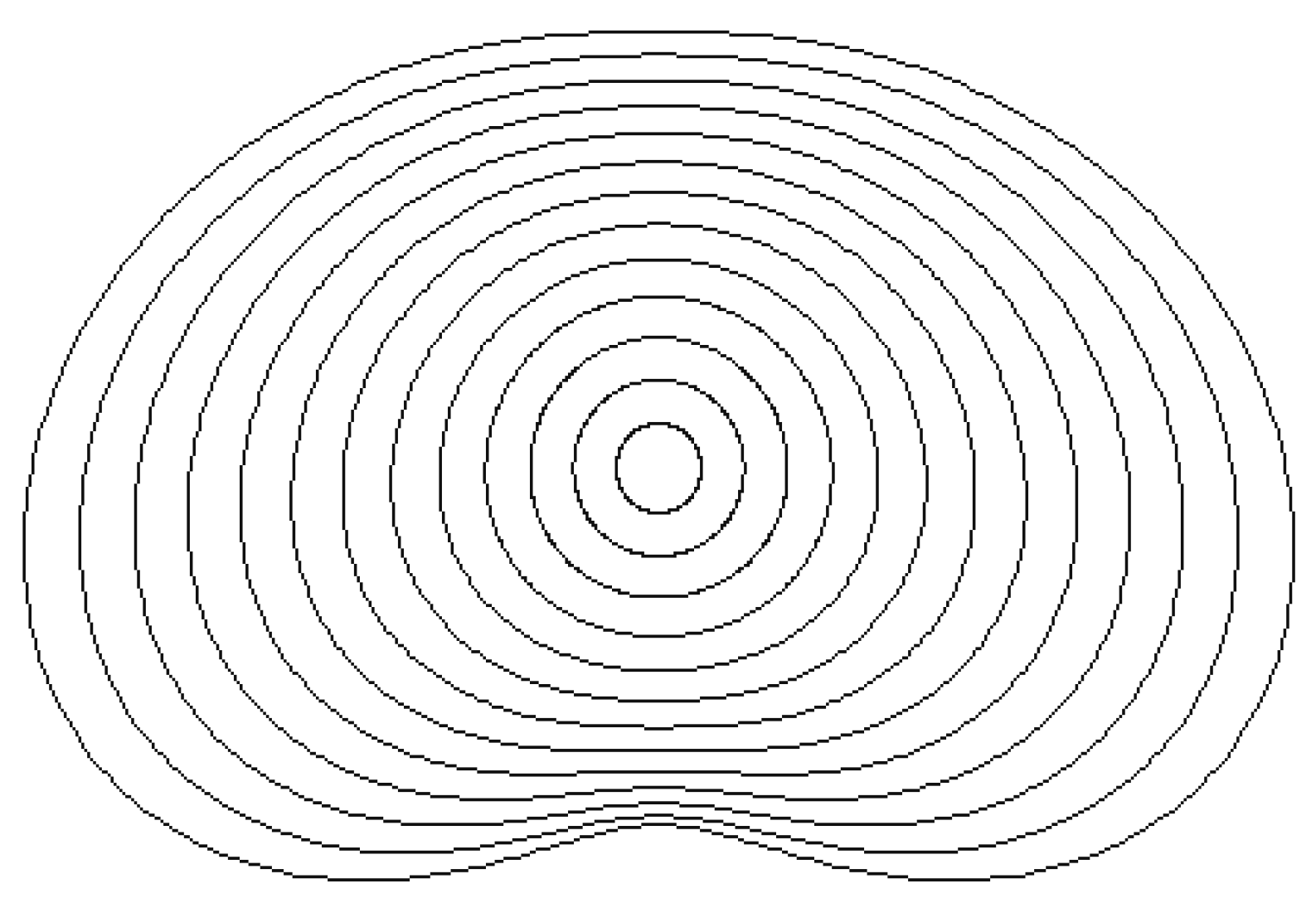
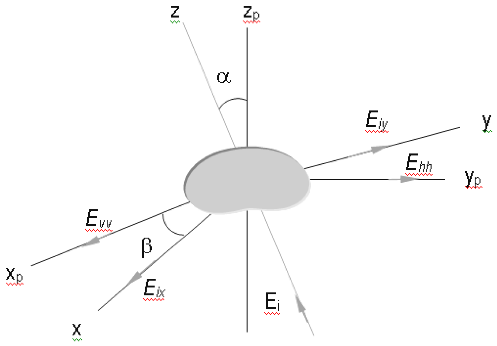
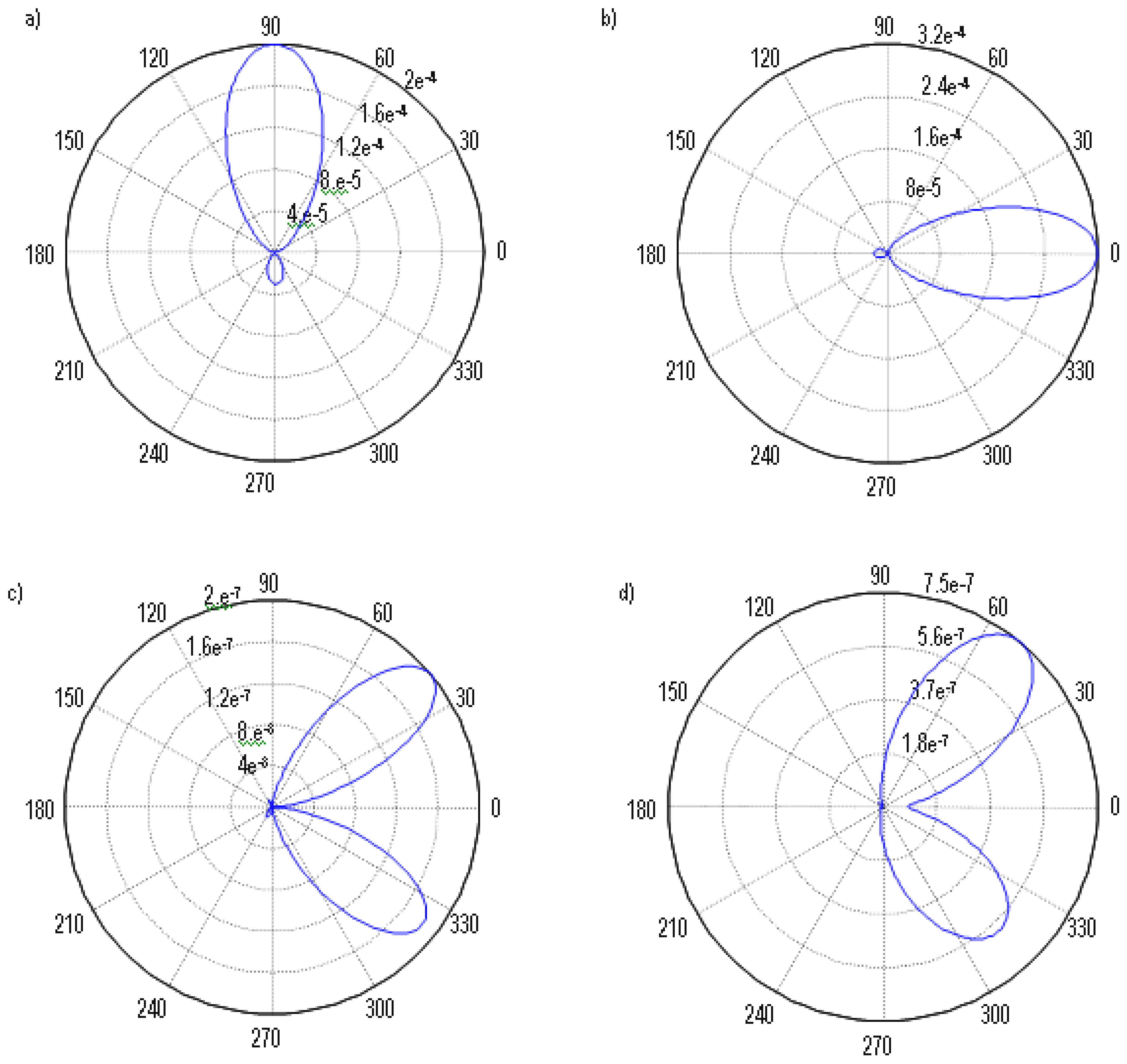
2.2. BEM Applied to Raindrop Scatterers

In order to apply Equation (8), the whole space is divided into two homogeneous regions (Figure 2a): region R1 inside the raindrop is water with permittivity ε1 and permeability μ0, and region R0 outside the raindrop is free space. The surface S refers to the boundary between R0 and R1.
The plane wave E i = e ^ i e j K 1 r incident on a drop located at the origin induces a field inside the drop and a scattered field E S outside the drops that in the direction K 2 is equal to:
E S = f ( K 1 , K 2 ) r e ^ s e j k r ,
where k=2π/λ0 is the free-space propagation constant, and f ( K 1 , K 2 ) is the vector scattering amplitude function that relates the amplitude, phase and polarization information of the scattered field relative to the incident one. This function is obtained from the solution of the boundary value problem at the surface of a raindrop.
The total fields are then the sum of the incident fields plus the scattered ones:
E T = E i + E S ,
H T = H i + H S .
For regions R0 and R1, Equation (8) can be written as:
[ D 0 ] [ H S 0 ] = [ C 0 ] [ E tan S 0 ] ,
[ D 1 ] [ H T 1 ] = [ C 1 ] [ E tan T 1 ] ,
and applying the boundary conditions over the surface S, (11a) and (11b) can be cast as:
[ D 0 C 0 D 1 C 1 ] [ H S 0 E tan S 0 ] = [ 0 [ C 1 ] [ E tan i ] [ D 1 ] [ H i ] ] .
Equation (12) is then solved using the conjugate-gradient method and the far fields are computed from the tangential field components over S (equivalent currents) and the vector scattering amplitudes.
Figure 2b presents the raindrop scattering geometry. The incident field is assumed to come from a direction forming an angle θ with respect to z ^ , and the drop axis is z ^ p ( z ^ p z ^ ). For θ = 0°, α is the drop canting angle (nutation) and β the angle between the azimuth of the direction of the incident electric field (direction of observation) and the wind speed (precession).
Figure 2a. Geometry of the scattering problem.
Remotesensing 01 00107 g002a
Figure 2b. Scattering by a raindrop: Electric incident field propagates along z ^ , drop axis along z ^ p , α: drop canting angle (nutation), and β: angle between the azimuth of the direction of observation and the wind direction (precession).
Remotesensing 01 00107 g002b
As an example, Figure 3 presents the bistatic scattering patterns in the XZ plane (see Figure 2b) computed using the BEM for 1.4, 2.56, 10.68, 19, 22, 37 and 94 GHz, for Pruppacher-Pitter raindrop shapes with different equivolumetric radii (Figure 1a) [4] for the case of incidence in the Z-direction and X-polarization. Figure 4 shows an example of the bistatic power scattering patterns at 34.8 GHz, in excellent agreement with Oguchi’s results [16,17].
Figure 4a and Figure 4b correspond to the patterns for the copolar scattered field in the vertical and horizontal planes, respectively. It should be pointed out that forward scattering is dominant, and that the drop shape asymmetry produces a slight difference in the amplitude of the two copolar scattered fields in the XZ and XY planes. Figure 4c and Figure 4d correspond to the cross-polar scattered field patterns, which are zero for spheroidal drops.
Figure 3. Scattering power patterns in the XZ plane for incidence from Z-direction (indicated by the arrow) at X-polarization, and different equivolumetric drop radii from 0.5 (inner curves) to 3.0 mm (outer curves) and frequencies: a) 1.4 GHz, b) 2.56 GHz, c) 10.68 GHz, d) 19.0 GHz, e) 22.0 GHz, f) 37.0 GHz, and g) 94.0 GHz. Plots normalized and in decibels, maximum value shown in each figure.
Remotesensing 01 00107 g003
Figure 4. Bistatic scattering power patterns in the XY plane of a Pruppacher-Pitter raindrop: Equivolumetric radius 3.0 mm, frequency 34.8 GHz. Polarizations of the incident and scattered waves are (a) vertical-vertical, (b) horizontal-horizontal, (c) vertical-horizontal, (d) horizontal-vertical.
Remotesensing 01 00107 g004

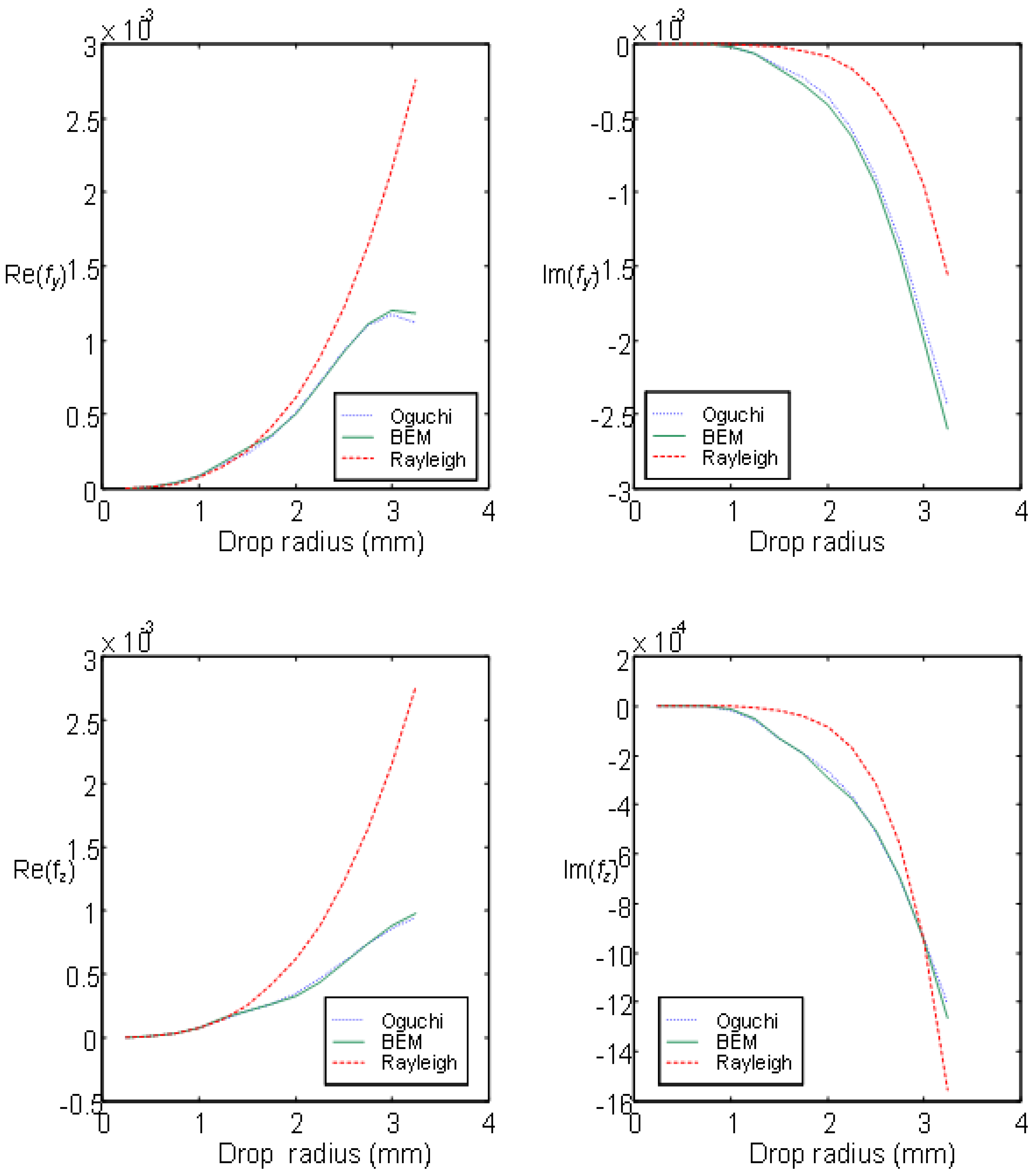
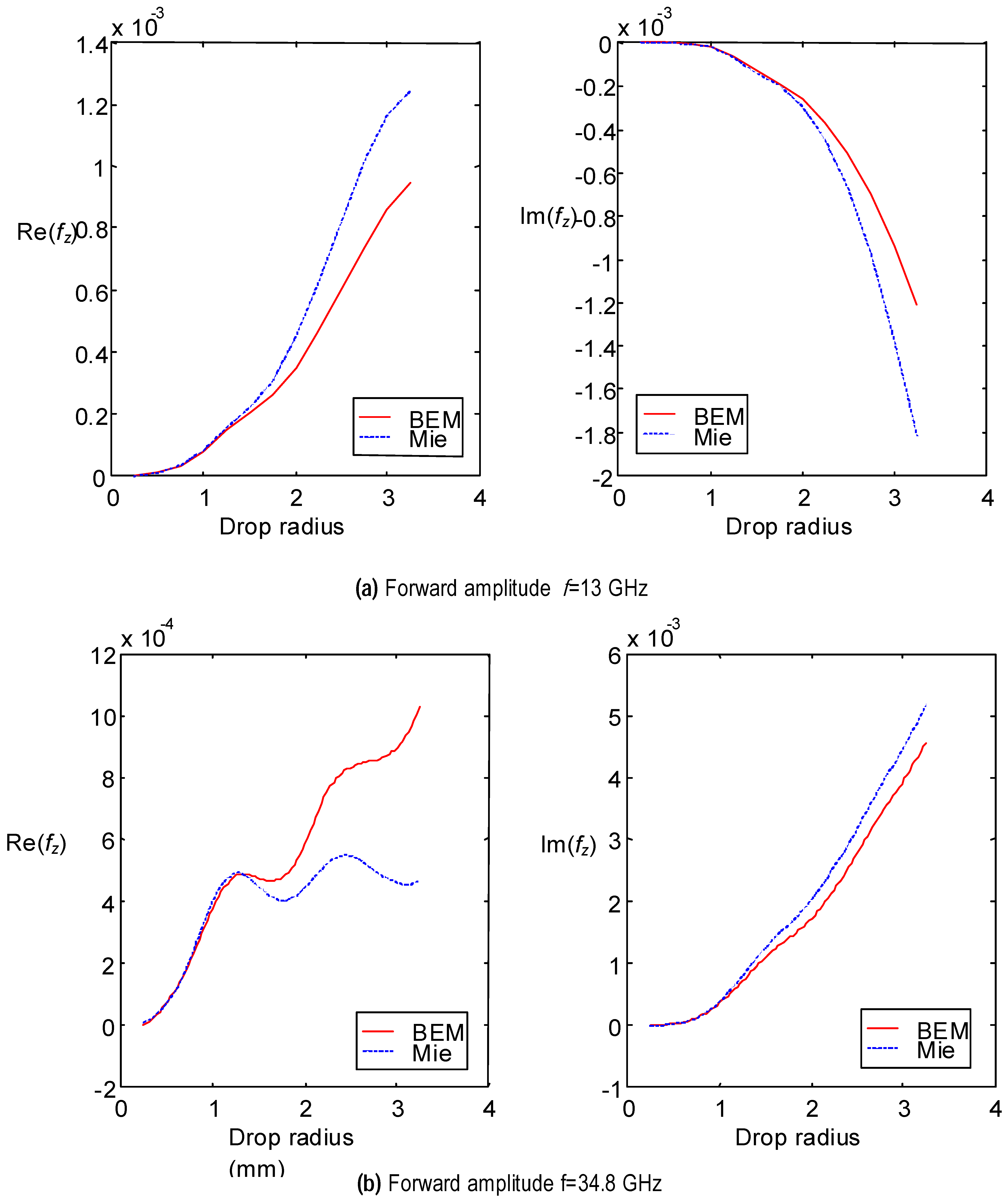
2.3. Inter-Comparison between Scattering Methods

An excellent agreement has been found between simulation results obtained with the boundary element method and Oguchi’s results [15] (Figure 5). At 13 GHz, forward scattering amplitudes computed using the Rayleigh approximation only agree with the BEM solution for drops up to 1 mm equivalent radius (Figure 5). Results computed at 13 GHz with Mie’s formulation approach the BEM results (Figure 6a) better than the Rayleigh’s ones (Figure 5), specially at large equivalent radius (> 2 mm). However, at higher frequencies (34.8 GHz), the scattering by the “kidney-bean” shaped raindrops deviates too much from Mie’s solution and the real part of the scattering functions are underestimated (Figure 6b), while BEM and Oguchi’s results keep showing an excellent agreement [17].
Figure 5. Real and imaginary parts of the amplitude scattering functions vs. raindrop radii at 13 GHz. Direction of propagation of the incident wave: x ^ , horizontal ( y ^ ) and vertical polarizations ( z ^ ). BEM solution (solid line) agrees well with Oguchi [15] (dotted line) for raindrops up to 3.25 mm radius. Rayleigh solution (dashed line) agrees with BEM solution up to 1 mm.
Remotesensing 01 00107 g005
Figure 6. Real and imaginary parts of the amplitude scattering functions vs. raindrop radii at 13 and 34.8 GHz. Direction of propagation of the incident wave: x ^ , vertical polarization ( z ^ ). BEM solution (solid line) shows an excellent agreement with Oguchi 1977 [17] (not shown), while Mie solution (dashed line) agrees only up to 1 to 1.5 mm radii.
Remotesensing 01 00107 g006

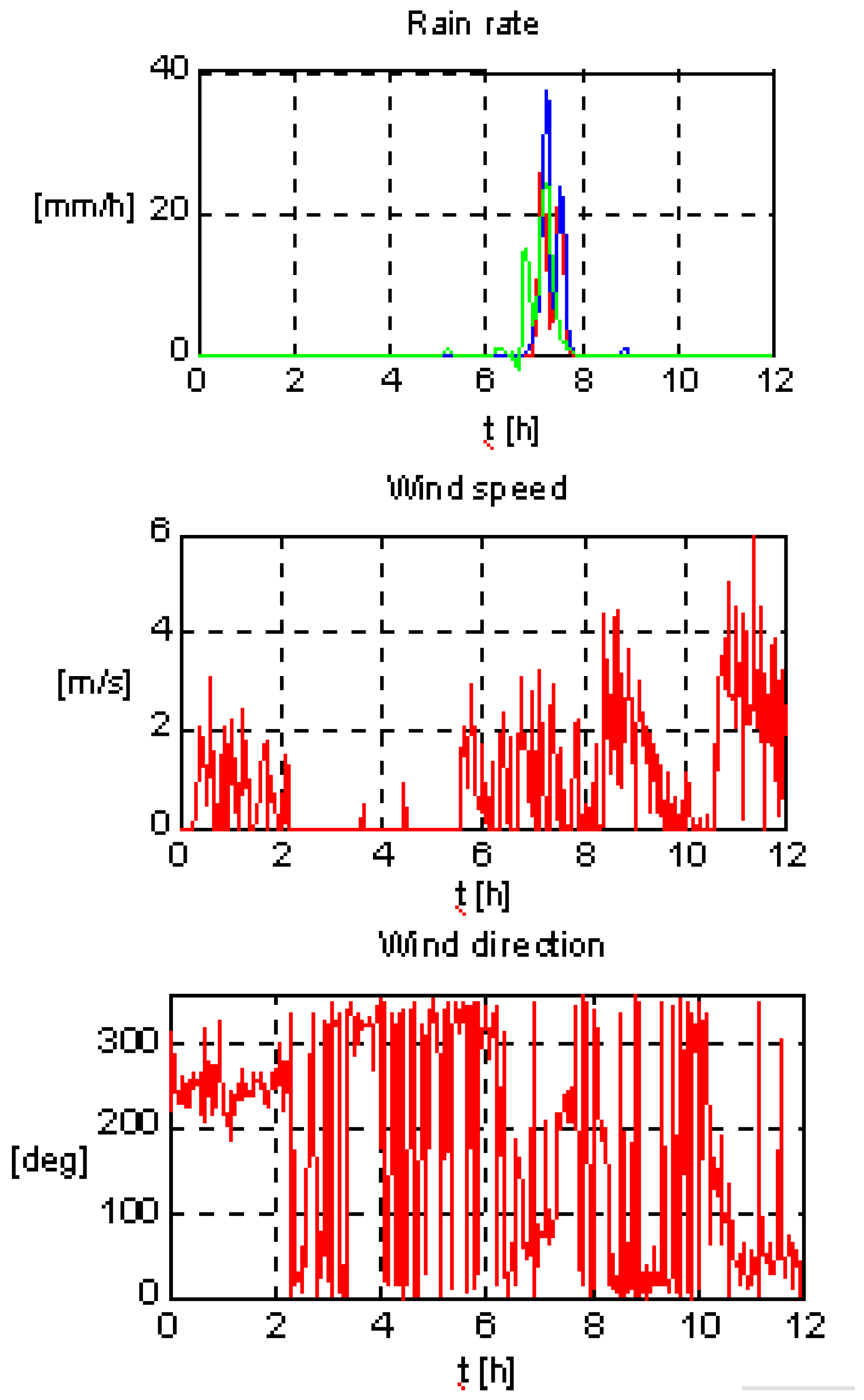
3. Polarimetric Emission of Rain Events

In the down-welling emission case, the boundary condition at the top of the atmosphere can be reasonably assumed to be T ¯ B ( θ , ϕ , z = h ) = [ 0   0   0   0 ] T . In order to solve Equation (1), the scattering functions have to be computed at arbitrary angles θ, α and β (Figure 2b), which depend on the observation geometry of the radiometer and the canting angles suffered by falling raindrops under a horizontal wind (In the presence of wind, raindrops migrate laterally within the air with negligible deformation and cant. For a constant shear flow in the horizontal direction, the axis of symmetry of the drop lies in the plane determined by the vertical direction and the wind speed vector, with a canting angle in the upwind direction. Depending on its size, the canting angle of the raindrop is estimated to be between 0º and 25º, but the average canting angle is just a few degrees).
The evaluation of equations (3-5) requires two steps:
a) computation of the scattering functions at incident polarization q and scattered polarization p, for each raindrop size according to the observation geometry and canting angle, and
b) averaging of the scattering functions over the ensemble of raindrop sizes according to its distribution:
< f p q > = 0 a max f p q ( a 0 ) N ( a 0 ) d a 0 ,
where a0 is the equivalent radius, and N (a0) is the Laws-Parsons drop size distribution [14].
Experimental data acquired with an X-band polarimetric radiometer developed at UPC [5, Figure 5] at 30° elevation are presented. Rain rate data was acquired every 5 minutes from three rain gauge stations of the Barcelona city network lying in the ground projection of the antenna beam (ΔθE3dB = 30°, ΔθH3dB = 20°), and from the meteorological station of the Institut de Tècniques Energètiques located on Campus, local rain rate was acquired every 30 s, while wind speed and direction were acquired every 5 seconds.
A rain event corresponding to August 18, 1998 is presented. The corresponding meteorological data is plotted in Figure 7. Figure 8 presents the simulated (left) and measured (right) Stokes parameters, respectively. The numerical modeling included data from the on Campus meteorological station only, since it was the one for which wind speed and direction were available. However, since the radiometer collects radiation from all the raindrops within its antenna beam, some peaks in the measured Stokes vector elements do not appear in the simulation results (Figure 8). The limited availability of wind speed and direction data does not allow to simulate better beam filling effects.
As expected, due to the flattened raindrop shape, the attenuation is slightly higher at horizontal polarization than at vertical polarization and therefore Th is slightly higher than Tv. Non-zero TU and TV parameters were also measured, although the values of TV are higher than expected, which can be attributed to a too simple modeling of the atmosphere or, probably, to the presence of ice particles that increase the differential phase shift between polarizations. In Figure 8, for high rain rates, changes in wind direction seem to be responsible for the amplitude modulation of Th and Tv.
Figure 7. Meteorological data of a rain event date August 18, 1998, 0-12 h.
Remotesensing 01 00107 g007
Figure 8. Simulation results (left) and radiometric measurements (right). Date: August 18, 1998, 0-12 h.
Remotesensing 01 00107 g008aRemotesensing 01 00107 g008b

4. Conclusions

This paper has presented the application of the Boundary Element Method (BEM) to the computation of the scattering functions of the fields scattered on Pruppacher Pitter raindrops with a Laws-Parsons distribution. Numerical simulations are in good agreement with the reported values up to 1-2 mm raindrop size. The accuracy of the method makes it suitable to evaluate the scattering functions of raindrops above 35 GHz, not reported in the literature. Simulation results show that:
a) raindrop shape is responsible for Th > Tv (at zero canting angle),
b) under horizontal winds, TU is originated by the cross-polarization of the emitted/attenuated radiation by raindrops rotated a certain canting angle (size dependent), and
c) TV is originated by the differential phase of the scattering amplitude functions between orthogonal polarizations.
The inter-comparison of simulation results with X-band experimental data is in good agreement except for the amplitude of the fourth Stokes vector element, higher than predicted, which can be probably originated by the phase shift difference originated by ice particles in the clouds.

Acknowledgements

This work has been supported by the Spanish “Comision Interministerial de Ciencia y Tecnología” and EU FEDER projects CICYT TEC2008-06764-C02, ESP2007-65667-C04-02 and AYA2008-05906-C02-01/ESP. The authors appreciate the meterological data provided by Dr. Guillem Cortés, Assistant Professor at ESCRA, Institut de Tècniques Energètiques, UPC.

References and Notes

  1. Liu, Q.; Weng, F.; Han, Y.; van Delst, P. Community Radiative Transfer Model for Scattering Transfer and Applications. In Proceedings of the IEEE International Geoscience & Remote Sensing Symposium, Boston, MA, USA, 2008; pp. 1193–1196.
  2. Yueh, S.H. Directional signals in windsat observations of hurricane ocean winds. IEEE Trans. Geosci. Remote. Sens. 2008, 46, 130–136. [Google Scholar] [CrossRef]
  3. Kutuza, B.G.; Zagorin, G.K.; Hornbostel, A.; Schroth, A. Physical modeling of passive polarimetric observations of the atmosphere with respect to the third stokes parameter. Radio Sci. 1998, 33, 677–695. [Google Scholar] [CrossRef]
  4. Hornbostel, A.; Schroth, A.; Sobachkin, A.; Kutuza, B.; Evtushenko, A.; Zagorin, G. Modelling and measurements of stokes vector microwave emission and scattering for a precipitating atmosphere. In Microwave Radiometry and Remote Sensing of the Earth's Surface and Atmosphere; VSP: Zeist, The Netherlands, 2000; pp. 313–324. [Google Scholar]
  5. Camps, A.; Vall-llossera, M.; Duffo, N.; Torres, F.; Barà, J.; Corbella, I.; Capdevila, J. Polarimetric Radiometry of Rain Events: Theoretical Prediction and Experimental Results, Microwave Radiometry and Remote Sensing of the Earth's Surface and Atmosphere; VSP: Zeist, The Netherlands, 2000; pp. 325–335. [Google Scholar]
  6. Tsang, L. Polarimetric passive microwave remote sensing of random discrete scatterers and rough surfaces. J. Electr. Wav. Appl. 1991, 5, 41–57. [Google Scholar]
  7. Smith, E.A.; Bauer, P.; Marzano, F.S.; Kummerow, C.D.; McKague, D.; Mugnai, A.; Panegrossi, G. Intercomparison of microwave radiative transfer models for precipitating clouds. IEEE Trans. Geosci. Remote Sens. 2002, 40, 541–549. [Google Scholar] [CrossRef]
  8. Randa, J.; Lahtinen, J.; Camps, A.; Gasiewski, A.; Hallikainen, M.; Le Vine, D.M.; Martin-Neira, M.; Piepmeier, J.; Rosenkranz, P.W.; Ruf, C.S.; Shiue, J.; Skou, N. Recommended terminology for microwave radiometry, NIST Technical Note TN1551. Available online: http://www.boulder.nist.gov/div818/81801/Noise/publications/TN1551.pdf (accessed in August 2008).
  9. Ishimaru, A. Electromagnetic Wave Propagation, Radiation and Scattering; Prentice Hall: Chandler, AZ, USA, 1991. [Google Scholar]
  10. Pruppacher, H.R.; Pitter, R.L. A semi-empirical determination of the shape of cloud and rain drops. J. Atmos. Sci. 1971, 28, 86–94. [Google Scholar] [CrossRef]
  11. Thurai, M.; Bringi, V.N. Drop axis ratios from a 2D video disdrometer. J. Atmos. Oceanic Technol. 2005, 22, 966–978. [Google Scholar] [CrossRef]
  12. Thurai, M.; Huang, G.J.; Bringi, V.N.; Randeu, W.L.; Schönhuber, M. Drop shapes, model comparisons, and calculations of polarimetric radar parameters in rain. J. Atmos. Oceanic Technol. 2007, 24, 1019–1032. [Google Scholar] [CrossRef]
  13. Thurai, M.; Szakáll, M.; Bringi, V.N.; Beard, K.V.; Mitra, S.; Borrmann, S. Drop shapes and axis ratio distributions: comparison between 2-D video disdrometer and wind-tunnel measurements. J. Atmos. Oceanic Technol. 2009. In Press. [Google Scholar] [CrossRef]
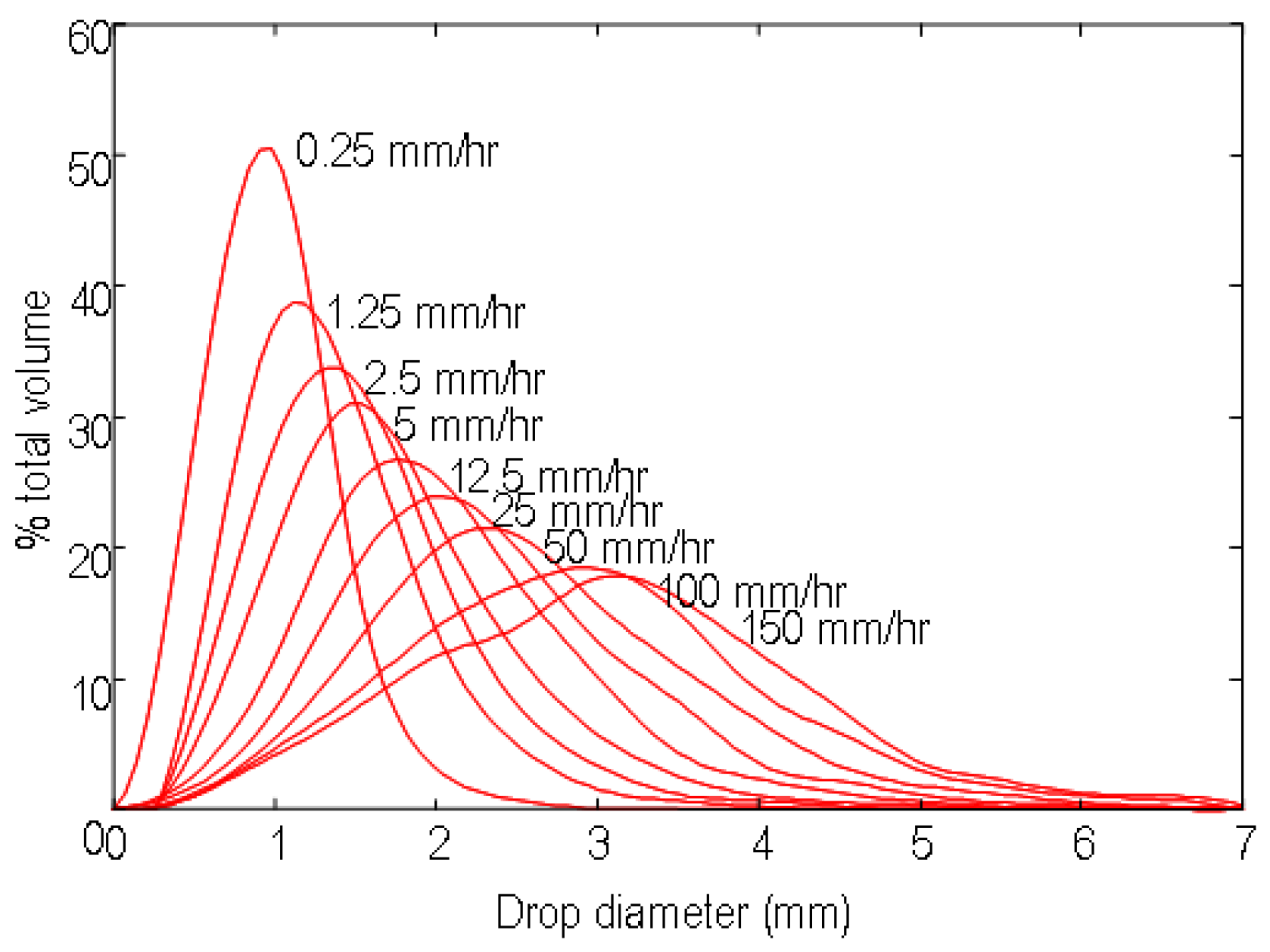
  14. Laws, J.O.; Parsons, D.A. The relationship of raindrops size to intensity. Trans. AGU. 1943, 24, 452–460. [Google Scholar] [CrossRef]
  15. Oguchi, T. Attenuation and phase rotation of radio waves due to rain: calculations at 19.3 and 34.8 GHz. Radio Sci. 1973, 8, 31–38. [Google Scholar] [CrossRef]
  16. Oguchi, T. Scattering from hydrometeors: a survey. Radio Sci. 1981, 16, 691–730. [Google Scholar] [CrossRef]
  17. Oguchi, T. Scattering properties of pruppacher-and-pitter form raindrops and cross polarization due to rain: calculations at 11, 13, 19.3 and 34.8 GHz. Radio Sci. 1977, 12, 41–51. [Google Scholar] [CrossRef]
  18. Paulsen, K.D.; Lynch, D.R.; Strohbehn, J. W. Three-dimensional finite, boundary, and hybrid element solutions of the maxwell equations for lossy dielectric media. IEEE Trans. Microwave Theory 1988, 36, 682–693. [Google Scholar] [CrossRef]

