Article

Mapping Invasive Tamarisk (Tamarix): A Comparison of Single-Scene and Time-Series Analyses of Remotely Sensed Data

by
Paul H. Evangelista
1,*,
Thomas J. Stohlgren
2,
Jeffrey T. Morisette
2 and
Sunil Kumar
1
1
Natural Resource Ecology Laboratory, Colorado State University, Fort Collins, Colorado 80523- 499, USA
2
U.S. Geological Survey, Fort Collins Science Center, Fort Collins, Colorado 80526, USA
*
Author to whom correspondence should be addressed.
Remote Sens. 2009, 1(3), 519-533; https://0-doi-org.brum.beds.ac.uk/10.3390/rs1030519
Submission received: 23 June 2009 / Revised: 14 August 2009 / Accepted: 21 August 2009 / Published: 31 August 2009
(This article belongs to the Special Issue Ecological Status and Change by Remote Sensing)

Abstract

:
In this study, we tested the Maximum Entropy model (Maxent) for its application and performance in remotely sensing invasive Tamarix sp. Six Landsat 7 ETM+ satellite scenes and a suite of vegetation indices at different times of the growing season were selected for our study area along the Arkansas River in Colorado. Satellite scenes were selected for April, May, June, August, September, and October and tested in single-scene and time-series analyses. The best model was a time-series analysis fit with all spectral variables, which had an AUC = 0.96, overall accuracy = 0.90, and Kappa = 0.79. The top predictor variables were June tasselled cap wetness, September tasselled cap wetness, and October band 3. A second time-series analysis, where the variables that were highly correlated and demonstrated low predictive strengths were removed, was the second best model. The third best model was the October single-scene analysis. Our results may prove to be an effective approach for mapping Tamarix sp., which has been a challenge for resource managers. Of equal importance is the positive performance of the Maxent model in handling remotely sensed datasets.

1. Introduction

Mapping invasive plant species has become a high priority for resource managers and researchers across the United States. Ground surveys are still commonly used for most mapping projects despite intensive labor requirements, associated high economic costs, and incomplete coverage of the landscape [1,2]. Improved methods to accurately determine the current distribution of invaders are required to better assess their environmental impacts, formulate effective control strategies, and forecast potential spread. Remote sensing has played an important, but limited, role in detecting and mapping invasive plants [3,4,5]. It is more commonly applied to mapping weeds in agricultural environments where species richness and diversity are minimal [6,7]. Detecting a specific plant species in forests, rangelands, riparian areas and natural landscapes using remote sensing techniques has proved to be a greater challenge. Large-scale infestations, where invaders are clearly the dominant species and environmental heterogeneity is reduced, tend to be easier to detect remotely [3,8,9].
One invasive plant that is especially problematic in the western U.S. is tamarisk (Tamarix spp.). Tamarisk is a small shrub-like tree that tends to grow in large monotypic stands along riparian corridors. A native to Eurasia and North Africa, tamarisk was introduced to North America in the late 1800s [10,11]. There are eleven species of tamarisk and at least three hybrids that have since become well established in the Americas, from Canada to Argentina [12]. Tamarisk’s impacts to native ecosystems in the U.S. include the desiccation of water tables, displacement of native plant communities, alteration of soil chemistry and ecosystem processes, and loss of critical wildlife habitat [13,14,15]. Infestations often begin discretely among species-rich riparian ecosystems before abruptly overwhelming and displacing competitor species. Once tamarisk establishes dominance, control and restoration efforts can be extremely labor intensive and costly. Detecting tamarisk in the early stages of infestation and mapping its distribution are essential to resource management and stewardship. Remote sensing of tamarisk distributions has been only marginally effective [16,17,18,19]. New airborne and satellite sensors promise to improve our ability to spectrally distinguish tamarisk from other species, but the techniques remain inadequate and are not yet economically practical.
The detection of invasive plants using remote sensing may be improved if the target species has phenological attributes that are distinctive from native vegetation. For example, leafy spurge (Euphorbia esula L.) has yellow-green inflorescences that are spectrally unique when compared to associated flora [4,20,21]. Similarly, yellow starthistle (Centaurea solstitialis), tamarisk (Tamarix spp.), yellow hawkweed (Hieracium pratense), oxeye daisy (Chrysanthemum leucanthemum), and Chinese tallow (Sapium sebiferum) also have distinctive colorations that can facilitate remote sensing [22,23,24]. Other species have been detected by their extended growing periods. Broom snakeweed (Gutierrezia sarothrae), a perennial sub-shrub, has been remotely sensed during its early-season greening [25]. Cheatgrass (Bromus tectorum), an invasive annual grass, has also been successfully detected because it germinates in winter months prior to most native grasses [26]. The distinctiveness of any phenological attribute can vary widely with regional climate, latitudinal gradients, and species richness within an ecosystem. As a result, the timing of acquiring remotely sensed data is critical and can be difficult to predict.
Time-series analyses of remotely sensed data have been widely used for mapping land cover and ecosystem types and are increasingly being used for detecting broad-scale invasions [27,28] and monitoring the impacts of mitigation treatments [29,30]. A few studies using time-series analyses have reported success in identifying cheatgrass. Bradley and Mustard [26] demonstrated how inter-annual data collected from Landsat and Advanced Very High Resolution Radiometer (AVHRR) can detect cheatgrass responses to precipitation. Peterson [31] was able to distinguish cheatgrass from other vegetation by using scenes from Landsat 7 ETM+ on two different dates within a single year. In both cases, the researchers were able to exploit subtle phenological differences (i.e., extended growing season, rapid response) between the invaders and associated native flora within a growing season. To determine the optimal time of the year to conduct remote sensing surveys, Everitt and Deloach [22] used a time-series of conventional color and color infrared aerial photographs for tamarisk and native riparian vegetation. From their study sites in Texas and Arizona, they found that tamarisk could best be identified in late fall and early winter months when foliage turned a yellow-orange color before dropping.
Remote sensing of tamarisk has had limited success, and conventional methods (e.g., supervised and unsupervised classification) have not proved to be reliable. Ge et al. [32] analyzed color aerial photographs at 1-m2 resolution using a texture analysis for tamarisk in northern California. The photographs were acquired in April and the mean grey-level values were calculated for 60 pixels representing eight cover types. They found that color alone could not distinguish tamarisk from associated vegetation; however, the use of textural classifiers greatly improved separability of cover types. In southern California, Hamada et al. [18] used discriminant analyses of presence/absence data and hierarchical clustering with hyperspectral imagery collected in October. Overall accuracy of their research varied by scene and minimum patch size, and results tended to over classify tamarisk distribution. Akasheh et al. [33] used an iterative classification procedure to map riparian vegetation with high-resolution multi-spectral airborne sensors in July on the Rio Grande River, New Mexico. The vegetation in their study site was largely dominated by four riparian species: tamarisk, cottonwood, willow, and Russian olive. Using 24 validation plots for tamarisk, they were able to achieve 86% classification accuracy.
These studies demonstrate an evolution of remote sensing and image processing for detecting tamarisk and other invasive species. The development of new airborne and satellite sensors and platforms, coupled with advanced statistical software, geographic information systems (GIS), and predictive models, give researchers a variety of tools to detect and predict the distribution of invasive species [34,35]. In this study, we explored the application of maximum entropy modeling with remotely sensed data to map the distribution of tamarisk while incorporating strategies that have been previously proven to be effective in vegetation mapping. Because conventional methods of remote sensing have limited applications for detecting tamarisk, our analyses were conducted using the Maxent software (v3.2.1; www.cs.princeton.edu/~schapire/maxent/), which uses presence points to predict the potential range and habitat distribution of a species [36,37]. In several recent studies, Maxent has been found to be especially useful for mapping invasive species [38,39] and ranked high when compared to other models for predicting tamarisk distributions [35]. We tested six satellite scenes and derived vegetation indices from different months of the growing season to detect tamarisk using single-scene and time-series analyses. Our objectives were to compare each analysis and determine which month of the growing season was the best time for detecting tamarisk. Lastly, we examined the effectiveness of several vegetation indices derived from remote sensing data that have proven useful in other remote sensing studies.

2. Methods

2.1. Study Area

This study was conducted in the lower Arkansas River in Southwestern Colorado. The Arkansas River is the sixth longest river in the continental U.S. Its headwaters begin in the Rocky Mountains of central Colorado and it flows 2,364 km east through Kansas, Oklahoma and Arkansas before emptying into the Mississippi River. In Colorado, the river drops 1,400 m in elevation from its origin to the edge of the Great Plains near the city of Pueblo [40]. From Pueblo, the river flows approximately 400 km to the Kansas state line and sustains a wide belt of irrigated agriculture through a series of ditches and channels. Elevations and mean annual precipitation range from 1,417 m and 29.7 cm at Pueblo to 1,021 m and 38.3 cm at the state line [41]. Tamarisk was first reported in this region in 1913, and observers noted the species’ rapid spread as early as 1921 [41]. Today, tamarisk infestation along the Arkansas River between Pueblo and the state line is estimated to be more than 120 km2 resulting in the estimated loss of 47,000 acre-feet of water annually [42].
Our study area was defined by the boundaries of the Landsat7 Enhanced Thematic Mapper Plus (ETM+) scene (Path 32, Row 34) used in our analyses. The study area includes approximately 175 km of the Arkansas River in southeastern Colorado between the town of Avondale and the City of Lamar (Figure 1). Also included in the scenes are John Martin Reservoir, the lower sections of the Purgatoire and Apishapa rivers, developed agricultural lands, and a significant area of semi-arid rangeland that extends into New Mexico.
Figure 1. Map of the Arkansas River in Colorado. The study area is highlighted in grey.
Remotesensing 01 00519 g001

2.2. Field Data

This study relied on the results of an intensive inventory and mapping effort by the Tamarisk Coalition (www.tamariskcoalition.org) and other groups completed in 2007. Inventory and mapping were coordinated with the U.S. Geological Survey’s (USGS) efforts to establish a national on-line database conforming to the weed mapping standards developed by the North American Weed Management Association (http://www.nawma.org/). This study utilized existing aerial photography, satellite imagery, and supplemental information available from multiple resource management agencies, research institutions and non-government organizations [42]. Stands of tamarisk were inventoried by field crews to confirm infestation density, maturity, height, accessibility, presence of native species, and other site characteristics. Stands of tamarisk were inventoried using global positioning systems (GPS) handheld units and transformed into spatially referenced geographical information systems (GIS) polygons with the aid of aerial photography. Over 1,633 miles of the Arkansas River, its tributaries, wetlands, and canals and dry land stands in the Arkansas watershed were surveyed [42], including the area in Colorado occupied by our imagery. These data are now stored and available on the National Institute of Invasive Species Science website (www.niiss.org). From these polygon data, we randomly generated 400 presence points from tamarisk polygons that had a percent basal cover >50%. Of these, 250 points were used for training (62.5%) the model, while 150 points were reserved for testing (37.5%). Some of our model testing required the use of absence points. An additional 150 tamarisk absence points were randomly generated using GIS for areas outside tamarisk polygons. These areas represent dry upland, agriculture, rangeland, and riparian land cover types.

2.3. Remotely Sensed Data

We used six Landsat 7 ETM+ scenes for our analyses. Each scene and derived vegetation indices were processed using ERDAS Imagine v9.0 [43] and ArcGIS 9.1 [44] software. The scenes, selected for their seasonal variation, were acquired on April 16, 2000; May 11, 2003; June 23, 2001; August 12, 2002; September 7, 2000; and October 23, 1999. From each scene, bands 1-5 and band 7 were used in our analyses. Additionally, we generated several vegetation indices from each scene that are commonly used for estimating vegetation and land-cover features. Normalized difference vegetation index (NDVI) is a non-linear transformation of the ratio between the visible (red) and near-infrared bands (NIR; [45]). The NDVI is commonly used to measure vegetation canopy characteristics such as biomass, leaf area index, and canopy cover [46,47,48]). We calculated NDVI using the following expression:
NDVI=(band 4 – band 3)/(band 4 + band 3)
The Ratio Vegetation Index (RVI) was calculated by dividing near infrared (band 4) by visible red (band 3) reflectance values [49]. The RVI and NDVI are very similar in that they are a measure of the slope of the line between the origin of red-NIR space and the red-NIR value of each pixel. The major difference between the two is the range of values given by the calculations. Some studies have used RVI and NDVI together [50], while other studies have elected to use one or the other [7].
Tasselled Cap transformations were conducted for each scene using the coefficients reported by Huang et al. [51]. Originally developed for understanding changes in crop development, tasselled cap transformations are weighted composites of the six Landsat bands into three orthogonal bands that have been useful in measuring soil brightness (tasselled cap, band 1), vegetation greenness (tasselled cap, band 2), and soil/vegetation wetness (tasselled cap, band 3, [52]). These transformations have been described as a guided and scaled principal components analysis and have been shown to be useful in identifying forest attributes such as species composition, age class, and structure [43,53,54].
We also calculated the Soil-Adjusted Vegetation Index (SAVI; [55]), a ratio-based index developed to minimize the effects of the soil background. The formula used for calculating SAVI is:
SAVI = [(band 4 – band 3) × (1 + L)/(band 4 + band 3 + L)]
where L is a correction factor ranging from 0 (high vegetation cover) to 1 (low vegetation cover). Each month had twelve potential predictor variables used for single-scene analyses, while the time-series analysis used a total of seventy-two potential predictor variables.

2.4. Data Analyses

We conducted our analyses using the Maxent software v.3.2 (www.cs.princeton.edu/~schapire/maxent/), which is a general-purpose method for estimating probability of distributions based on the principle of maximum entropy [36,37]. Maxent uses presence-only data to define known conditions within the parameters of the independent variables to predict a species’ distribution and excludes all conditions that are unfounded or undefined. The model is nonlinear, nonparametric, and not sensitive to multicollinearity. Besides having several evaluation features built into the program, Maxent also provides the percent contribution of each predictive variable. Several recent studies have found the Maxent model to perform as well, or better, when compared to other modeling methods [35,39,56].
Each monthly scene, and the associated vegetation indices, were analyzed and tested independently (six models); while the time-series analyses were conducted using two modeling procedures. The first time-series model used all 72 predictor variables generated from the six scenes. From these results, we restricted the models to only those variables that had a predictive contribution >1.0% (n = 17) and used them as predictor variables for our second time-series model. The 17 variables were tested for cross-correlations using SYSTAT (version 12; SYSTAT Software, Port Richmond, California, USA). For variables that were highly correlated (Pearson correlation coefficient >0.80), we removed the ones that had the least predictive contribution in first-time series analysis model. This further reduced our number of variables to seven potential predictors.
We tested the models with threshold-dependent and threshold-independent measures using features available with Schroder’s ROC/AUC software (http://brandenburg.geoecology.uni-potsdam.de/users/schroeder/download.html). The ROC/AUC software was specifically developed for assessing the predictive performance of habitat models and requires presence and absence data. Threshold-dependent evaluations, using the ROC/AUC software, were measured by specificity, sensitivity, and Cohen’s maximized Kappa [57]. Specificity is the proportion of true-positive and false-positive absences, and sensitivity is the proportion of true-positives and false-positive presences. The maximized Kappa statistic (K) measures the proportion of correctly classified points (i.e., presence, absence) after accounting for the probability of chance agreement. Kappa statistic values range from –1 to +1, where +1 would be perfect agreement, and any values less than 0 would indicate a performance no better than random [57,58]. Landis and Koch [59] ranked analysis performances as poor when Kappa values are <0.40, good when the Kappa values range from 0.40 to 0.75, and excellent when Kappa values are >0.75.
The threshold-independent evaluation required a Receiver Operating Characteristic (ROC) curve, where ‘sensitivity’ is plotted against ‘1-specificity’ for all possible thresholds [60]. From the ROC analysis, the Area under the ROC Curve (AUC) is calculated using presence and absence observations to measure the probability that a random, positive point falls within the predicted range of occurrence, and a random negative point falls outside [61]. The AUC value can vary from 0.5 (no better than random) to 1.0 (perfect discrimination, [62]). AUC evaluations for each model are presented in the results.

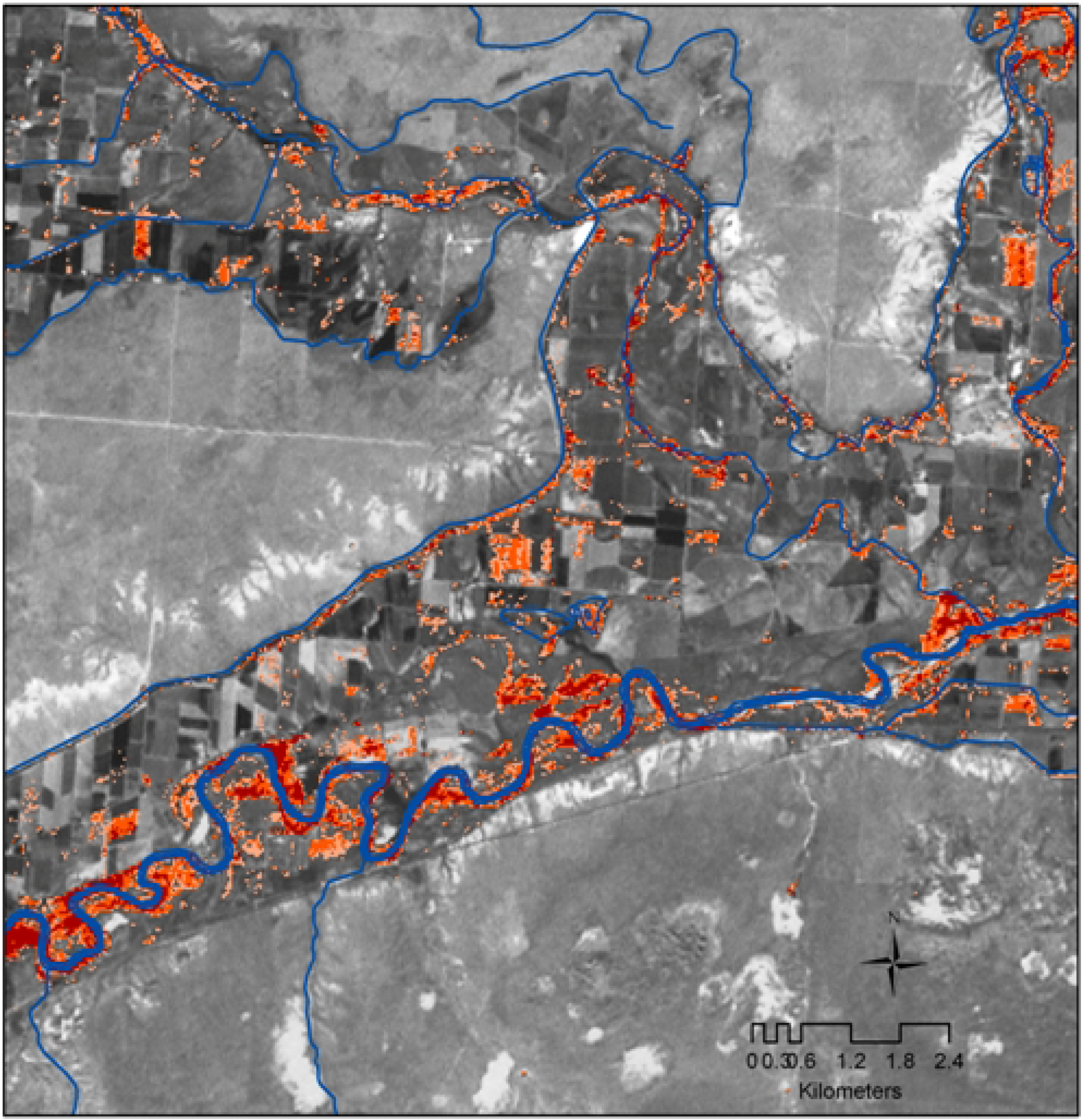
3. Results and Discussion

All the models generally performed well, further highlighting the applicability of remote sensing and vegetation indices for detecting tamarisk. The best model was the first time-series analysis that used all 72 variables (Figure 2). The AUC value for this model was 0.96, while the percent of correct predictions was 0.90 and kappa statistic was 0.79 (Table 1). The next best models were the second time-series analyses with the reduced number of variables, and the October single-scene analysis. The AUC values for these models were 0.93 and 0.89, respectively. The percent of correct predictions and kappa statistics for the second time-series analyses and October single-scene analyses were 0.84 and 0.85, and 0.69 and 0.71, respectively. The June, August, and September single-scene analyses had slightly lower but similar evaluations. Generally, the results from the single-scene analyses improved toward the later part of the growing season and into the fall months when most native plants go into dormancy.
Table 1. Tamarisk model evaluations of single-scene and time-series analyses of Landsat 7 scenes and associated vegetation indices generated using the ROC/AUC Calculator.
Scene analysisNum. variablesAUCSensitivitySpecificity% CorrectKappa
April120.890.750.890.820.64
May120.880.830.840.830.67
June120.920.930.760.840.69
August120.910.910.790.850.70
September120.910.830.890.860.71
October120.890.770.940.850.71
Time-series1720.960.930.860.900.79
Time-series270.930.850.840.840.69
Figure 2. An enlarged view of tamarisk detected along the Arkansas River and irrigation ditches near the town of Riverdale in southeastern Colorado. The results shown here are from a time-series analysis that used 72 remotely sensed data sets from Landsat 7 ETM+. Tamarisk infestations are shown from moderate (orange) to high (red).
Remotesensing 01 00519 g002
The best predictor variables for the first time-series analyses were the June tasselled cap wetness (25.8%), September tasselled cap wetness (16.4%), and October wetness (11.6%, Table 2). Similarly, the best predictors for the second time-series analyses were the June tasselled cap wetness (63.1%), April NDVI (9.7%), and October band 3 (7.8%). It should be noted that the September tassled cap band 3 was found to be highly correlated with the June tasselled cap wetness, thus it was omitted from the second time-series analyses. With the exception of the April NDVI, the best predictors for both time-series analyses were from the months that performed the best of the six single-scene analyses. Of the eight models, seven had at least one tasselled cap transformation as one of the top predictors.
Table 2. The predictive contributions of the top three variables for each model generated from Maxent.
Scene AnalysisVariableContribution (%)
Aprilband 725.5
band 420.6
NDVI17.8
Mayband 7 37.7
tasselled cap wetness31.9
band 19.9
Junetasselled cap wetness78.5
band 18.6
band 45.5
Augusttasselled cap wetness59
band 413.6
band 19.6
Septembertasselled cap wetness42.2
band 516.1
band 714.3
Octoberband 330.2
tasselled cap wetness21.4
band 717.9
Time-series1(June) tasselled cap wetness25.8
(Sept) tasselled cap wetness16.4
(Oct) band 311.6
Time-series2(June) tasselled cap wetness63.1
(April) NDVI9.7
(Oct) band 37.8
Our results suggest that the time-series analyses can better distinguish phenological differences between tamarisk and native flora than a single-scene analysis (Table 1). Spectral data from the months of June, September, and October consistently had the greatest capability for detecting tamarisk in all of our models. We can speculate that the peak in tamarisk green-up and its purple-pink flowers contribute to the spectral uniqueness during June, while its extended growing season and the yellow foliage late in the year are conspicuous in September and October. Collectively, data from these months produced the strongest results in our time-series analysis; we are encouraged to see that they each performed exceptionally well with the single-scene analyses. Our findings are also in agreement with results from previous remote sensing studies on tamarisk [22,33]. Although spectral data from these months performed best in our study area, they may not necessarily be the best candidates in other ecosystems, geographic regions, or spatial scales.
Vegetation indices used in our analyses made considerable predictive contributions to our final results. Most notable were the tasselled cap transformations for soil/vegetation wetness (tasselled cap band 3). The tasselled cap wetness index has been shown in other studies to be reliable for detecting change in forest structure and biomass using single-scene and time-series analyses [54,63,64]. Tamarisk biomass in our study site is quite extensive and significantly higher than native vegetation [35]. Further study may be required to test the effectiveness of the tasselled cap wetness index on low densities of tamarisk; however, our results indicate the index may perform well with the remote sensing of large tamarisk stands or when used in a time-series analysis.
We were also encouraged by the performance of the Maxent model in analyzing remote sensing data. We are confident that our model results could be improved if we integrated additional geospatial variables that characterize the physical landscape (e.g., distance from water, slope), but we elected to analyze monthly scenes and vegetation indices exclusively to better identify temporal trends with tamarisk’s phenology in relation to other vegetation.

4. Conclusions

Our study revealed several important factors that may significantly improve the use of remotely sensed data for detecting tamarisk and other invasive species. Our time-series analysis using all 72 variables performed best, while our second time-series analysis using the seven best predictors that were not correlated had only a slight reduction in model performance. This would suggest that variables that have lower predictive contributions can still improve results when used collectively. We have identified at least three different times during the growing season when phenological attributes of tamarisk can help distinguish the species from native vegetation. We have also demonstrated that phenological differences may be better detected using a time-series analysis than a single-scene analysis. Biomass indicators, such as the tasselled cap wetness index, may prove useful for remotely sensing large tamarisk infestations or for detecting landscape change in a time-series analysis.
Our study also demonstrates that the Maxent model may prove to be a powerful new tool for analyzing remotely sensed data. Originally designed as a model for predicting species distribution and potential habitat, Maxent has several features that support remote sensing analysis. Maxent is not sensitive to multicollinearity, which is commonly associated with remotely sensed data sets. It also can be used with presence-only data and requires no additional partitioning of background data. Lastly, Maxent easily integrates other geospatial data types (elevation, distance from water) that may enhance prediction and detection efforts.
There are several caveats in regard to this study that need to be considered. First, tamarisk presence points used to train and test our models were randomly generated indirectly from GIS polygons derived from field surveys. Similarly, absence points required for some of our evaluations were randomly generated in areas where tamarisk was not reported to occur. These methods may increase the risk of sampling error compared to other sampling designs. Although we are confident in the data quality from the Tamarisk Coalition’s survey efforts, we must recognize that this approach may not be the ideal sampling design for training Maxent models and remotely sensed data. For future efforts, we suggest that training and testing data be acquired by direct field observations with geographical coordinates collected on site. Specifically, each presence or absence point used for the analysis should be confirmed and recorded in the field to minimize sampling error and increase data quality.
Second, the training data selected for the analysis required that tamarisk have a minimum basal area of 50%, which we believed was an appropriate threshold for our tests given the resolution of Landsat 7 ETM+ scenes (i.e., 30 m2), the extent of our study area, and the uncertainty related to the field data. Thus, the presence data used to train our models were derived from areas where tamarisk was the dominant vegetation type. This presents obvious limitations for mapping tamarisk distributions and detecting early infestations. Our methods, however, can be easily modified to fit different management objectives and used with different types and formats of remotely sensed data. For example, smaller study areas may be better suited for high-resolution imagery, which would enhance the detection of individual plants and low-density infestations. This approach may prove to be too costly for resource management agencies that require surveys across large landscapes. Despite the fact that our results are only applicable where tamarisk is dominant, they are still valuable for planning mitigation efforts. For example, the use of bio-control agents and aerial spraying of herbicides is most economically feasible on large areas where tamarisk is dominant. Regardless, we must recognize that remote sensing of individual plants inhabiting diverse ecosystems still presents many challenges and limitations.
Despite these concerns, we believe that the methods tested in this research have produced promising results that will enhance our ability to remotely sense tamarisk and other invasive plant species. We have also found the Maxent model to perform positively when used with remotely sensed data. Further refinement of our methods is needed, including tests that employ different sensors across multiple spatial scales.

Acknowledgements

We would like to acknowledge the Tamarisk Coalition for the data contributions that made this study possible. We would also like to thank the Natural Resource Ecology Laboratory at Colorado State University and U.S. Geological Survey Fort Collins Science Center for analyses support; NASA Goddard Space Flight Center for providing remote sensing data; and the Colorado State Forest Service and Colorado Division of Wildlife for field assistance and logistical support. Any use of trade, product, or firm names is for descriptive purposes only and does not imply endorsement by the U.S. Government. Jim Graham and Alycia Crall were helpful for editorial comments on earlier versions of the manuscript. Finally we would like to thank N. Ament, T. Carlson, A. Randell, C. Tate, and S. VanLandingham. To all we are grateful.

References and Notes

  1. Crosier, C.S.; Stohlgren, T.J. Improving biodiversity knowledge with data set synergy: a case study of nonnative plants in Colorado. Weed Technol. 2004, 18, 1441–1444. [Google Scholar] [CrossRef]
  2. Dewey, S.A.; Anderson, K.A. Distinct roles of surveys, inventories, and monitoring in adaptive weed management. Weed Technol. 2004, 18, 1449–1452. [Google Scholar] [CrossRef]
  3. Anderson, G.L.; Everitt, J.H.; Richardon, A.J.; Escobar, D.E. Using satellite data to map false broomweed (Ericameria austrotexana) infestations on south Texas rangelands. Weed Technol. 1993, 7, 865–871. [Google Scholar]
  4. Everitt, J.H.; Anderson, G.L.; Escobar, D.E.; Davis, M.R.; Spencer, N.R.; Andrascik, R.J. Use of remote sensing for detecting and mapping leafy spurge (Euphorbia esula). Weed Technol. 1995, 9, 599–609. [Google Scholar]
  5. Rowlinson, L.C.; Summerton, M.; Ahmed, F. Comparison of remote sensing data sources and techniques for identifying and classifying alien invasive vegetation in riparian zones. Water SA 1999, 25, 497–500. [Google Scholar]
  6. Medlin, C.R.; Shaw, D.R.; Gerard, P.D.; LaMastus, F.E. Using remote sensing to detect weed infestations in Glycine max. Weed Sci. 2000, 48, 393–398. [Google Scholar] [CrossRef]
  7. Lopez-Granados, F.; Garcia-Torres, L. Using remote sensing for identification of late-season grass weed patches in wheat. Weed Sci. 2006, 54, 346–353. [Google Scholar]
  8. Lass, W.L.; Prather, T.S.; Glenn, N.F.; Weber, K.T.; Mundt, J.T.; Pettingill, J. A review of remote sensing of invasive weeds and example of the early detection of spotted knapweed (Centaurea maculosa) and babysbreath (Gypsophila paniculata) with a hyperspectral sensor. Weed Sci. 2005, 53, 242–251. [Google Scholar] [CrossRef]
  9. Laba, M.; Tsai, F.; Ogurcak, D.; Smith, S.; Richmond, M.E. Field determination of optimal dates for the discrimination of invasive wetland plant species using derivative spectral analysis. Photogramm. Eng. Remote Sensing 2005, 71, 603–611. [Google Scholar] [CrossRef]
  10. Carleton, M.A. Adaptation of the tamarisk for dry lands. Science 1914, 39, 692–694. [Google Scholar] [CrossRef] [PubMed]
  11. DiTomaso, J.M. Impact, biology, and ecology of saltcedar (Tamarix spp.) in the southwestern United States. Weed Technol. 1998, 12, 326–336. [Google Scholar]
  12. U.S. Department of Agriculture (USDA) Plants Database; Natural Resources Conservation Service. 2008. Available online: http://plants.usda.gov/ (accessed on August 28, 2009).
  13. Christiansen, E.M. The rate of naturalization of Tamarix in Utah. Am. Midl. Nat. 1962, 68, 51–57. [Google Scholar] [CrossRef]
  14. Robinson, T.W. Introduction, spread, and aerial extent of saldcedar (Tamarix) in the western states. In Professional Paper 491-A; U.S. Department of the Interior, Geological Survey: Washington, DC, USA, 1965; p. 11. [Google Scholar]
  15. Harris, D.R. Recent plant invasions in the arid and semi-arid Southwest of the United States. Ann. Assn. Amer. Geogr. 1966, 56, 408–422. [Google Scholar] [CrossRef]
  16. Lass, L.W.; Thill, D.C.; Shafii, B.; Prather, T.S. Detecting spotted knapweed (Centaurea maculosa) with hyperspectral remote sensing technology. Weed Technol. 2002, 16, 535–545. [Google Scholar] [CrossRef]
  17. Hirano, A.; Madden, M.; Welch, R. Hypersptectral image data for mapping wetland vegetation. Wetlands 2003, 23, 436–448. [Google Scholar] [CrossRef]
  18. Hamada, Y.; Stow, D.A.; Coulter, L.L.; Jafolla, J.C.; Hendricks, L.W. Detecting Tamarisk species (Tamarix spp.) in riparian habitats of Southern California using high spatial resolution hyperspectral imagery. Remote Sens. Environ. 2007, 109, 237–248. [Google Scholar] [CrossRef]
  19. Asner, G.P.; Jones, M.O.; Martin, R.E.; Knapp, D.E.; Hughes, R.F. Remote sensing of native and invasive species in Hawaiian forests. Remote Sens. Environ. 2008, 112, 1912–1926. [Google Scholar] [CrossRef]
  20. Williams, A.P.; Hunt, E.R., Jr. Estimation of leafy spurge cover from hyperspectral imagery using mixture tuned matched filtering. Remote Sens. Environ. 2002, 82, 446–456. [Google Scholar] [CrossRef]
  21. Hunt, E.R., Jr.; Everitt, J.H.; Ritchie, J.C.; Moran, M.S.; Booth, D.T.; Anderson, G.L.; Clard, P.E.; Seyfried, M.S. Applications and research using remote sensing for rangeland management. Photogramm. Eng. Remote Sensing 2003, 69, 675–693. [Google Scholar] [CrossRef]
  22. Everitt, J.H.; Deloach, C.J. Remote sensing of Chinese tamarisk (Tamarix chinensis) and associated vegetation. Weed Sci. 1990, 38, 273–278. [Google Scholar]
  23. Lass, L.W.; Carson, H.W.; Callihan, R.W. Detection of yellow starthistle (Centaurea solstitialis) and common St. Johnswort (Hypericum perforatum) with multispectral digital imagery. Weed Technol. 1996, 10, 466–474. [Google Scholar]
  24. Lass, L.W.; Callihan, R.H. 1997. The effect of phenological stage on detectability of yellow hawkweed (Hieracium pretense) and oxeye daisy (Chrysanthemum leucanthemum) with remote multispectral digital imagery. Weed Technol. 1997, 11, 248–256. [Google Scholar]
  25. Peters, A.J.; Reed, B.C.; Eve, M.D.; McDaniel, K.C. Remote sensing of broom snakeweed (Gutierrezia sarothrae) with NOAA-10 spectral image processing. Weed Technol. 1992, 6, 1015–1020. [Google Scholar]
  26. Bradley, B.A.; Mustard, J.F. Identifying land cover variability distinct from land cover change: cheatgrass in the Great Basin. Remote Sens. Environ. 2005, 94, 204–213. [Google Scholar] [CrossRef]
  27. Pavri, F.; Aber, J.S. Characterizing wetland landscapes: a spatiotemporal analysis of remotely sensed data at Cheyenne Bottoms, Kansas. Phys. Geogr. 2004, 25, 86–104. [Google Scholar] [CrossRef]
  28. Robinson, T.P.; van Klinken, R.D.; Metternicht, G. Spatial and temporal rates and patterns of mesquite (Prosopis species) invasion in Western Australia. J. Arid Environ. 2008, 72, 175–188. [Google Scholar] [CrossRef]
  29. Anderson, G.L.; Carruthers, R.I.; Ge, S.K.; Gong, P. Monitoring of invasive Tamarix distribution and effects of biological control with airborne hyperspectral remote sensing. Int. J. Remote Sens. 2005, 26, 2487–2489. [Google Scholar] [CrossRef]
  30. Everett, J.H.; Yang, C.; Fletcher, R.S.; Deloach, C.J.; Davis, M.R. Using remote sensing to assess biological control of saltcedar. Southwest. Entomologist 2007, 32, 93–103. [Google Scholar] [CrossRef]
  31. Peterson, E.B. Estimating cover of an invasive grass (Bromus tectorum) using tobit regression and phenology derived from two dates of Landsat ETM+ data. Int. J. Remote Sens. 2005, 26, 2491–2507. [Google Scholar] [CrossRef]
  32. Ge, S.; Carruthers, R.; Gong, P.; Herrera, A. Texture analysis for mapping Tamarix parviflora using aerial photographs along Cache Creek, California. Environ. Monit. Assess. 2006, 114, 65–83. [Google Scholar] [CrossRef] [PubMed]
  33. Akasheh, O.Z.; Neale, C.M.U.; Jayanthi, H. Detailed mapping of riparian vegetation in the middle Rio Grande River using high resolution multi-spectral airborne remote sensing. J. Arid Environ. 2008, 72, 1734–1744. [Google Scholar] [CrossRef]
  34. Morissette, J.T.; Jarnevich, C.S.; Ullah, A.; Cai, W.; Pedelty, J.A.; Gentle, J.E.; Stohlgren, T.J.; Schnase, J.L. A tamarisk habitat suitability map for the continental United States. Front. Ecol. Environ. 2006, 4, 11–17. [Google Scholar] [CrossRef]
  35. Evangelista, P.H.; Kumar, S.; Stohlgren, T.J.; Jarnevich, C.S.; Crall, A.W.; Norman, B.; Barnett, D.T. Modelling invasion for a habitat generalist and a specialist plant species. Divers. Distrib. 2008, 14, 808–817. [Google Scholar] [CrossRef]
  36. Phillips, S.J.; Dudik, M.; Schapire, R.E. A maximum entropy approach to species distribution modeling. In Proceedings of the 21st International Conference on Machine Learning; ACM Press: New York, NY, USA, 2004; pp. 655–662. [Google Scholar]
  37. Phillips, S.J.; Anderson, R.P.; Schapire, R.E. Maximum entropy modeling of species geographic distributions. Ecol. Model. 2006, 190, 231–259. [Google Scholar] [CrossRef]
  38. Ficetola, G.F.; Thuiller, W.; Miaud, C. Prediction and validation of the potential global distribution of problematic alien invasive species-the American bullfrog. Divers. Distrib. 2007, 13, 476–485. [Google Scholar] [CrossRef]
  39. Kumar, S.; Spaulding, S.A.; Stohlgren, T.J.; Hermann, K.A.; Schmidt, T.S.; Bahls, L.L. Potential habitat distribution for the freshwater diatom Didymosphenia geminata in the continental US. Front. Ecol. Environ. 2009, 7. [Google Scholar] [CrossRef]
  40. Kammerer, J.C. Largest Rivers in the United States. 1990. Available online: http://pubs.usgs.gov/of/1987/ofr87-242/ (accessed on August 28, 2009). [Google Scholar]
  41. Lindauer, I.E. A comparison of the plant communities of the South Platte and Arkansas River drainages in eastern Colorado. Southwest. Naturalist 1983, 28, 249–259. [Google Scholar] [CrossRef]
  42. Tamarisk Coalition. Riparian Restoration: Assessment of alternative technologies for tamarisk control, biomass reduction and revegetation. 2008. Available online: http://www.tamariskcoalition.org (accessed on August 28, 2009).
  43. Leica. ERDAS Imagine 9.1; Leica Geosystems Geospatial Imaging, LLC: Atlanta, GA, USA, 1991–2005. Available online: http://www.erdas.com/Leica.
  44. ESRI. ArcGIS 9.1; ESRI: Redlands, CA, USA, 2004. Available online: http://www.esri.com/index.html (accessed on August 28, 2009).
  45. Rouse, J.W.; Haas, R.H.; Schell, J.A.; Deering, D.W. Monitoring vegetation systems in the Great Plains with ERTS. In Proceedings of the Third Earth Resources Technology Satellite-1 Symp., Greenbelt, MD, USA, 1974.
  46. Kriegler, F.J.; Malila, W.A.; Nalepka, W.A.; Richardson, W. Preprocessing transformations and their effects on multispectral recognition. In Proceedings of the Sixth International Symposium on Remote Sensing of Environment; University of Michigan: Ann Arbor, MI, USA, 1969; pp. 97–131. [Google Scholar]
  47. Myneni, R.B.; Ramakrishna, R.; Nemani, R.; Running, S.W. Estimation of global leaf area index and absorbed par using radiative transfer models. IEEE Geosci. Remote Sens. 1997, 35, 1380–1393. [Google Scholar] [CrossRef]
  48. Todd, S.W.; Hoffer, R.M.; Milchunas, D.G. Biomass estimation on grazed and ungrazed rangelands using spectral indices. Int. J. Remote Sens. 1998, 19, 427–438. [Google Scholar] [CrossRef]
  49. Jordan, C.F. Derivation of leaf area index from quality of light on the forest floor. Ecology 1969, 50, 663–666. [Google Scholar] [CrossRef]
  50. Liu, W.G.; Gao, W.; Gao, Z.Q.; Wang, X.L.; Slusser, J. An analysis between the biomass of ecosystem of oasis and the vegetation index. In Remote Sensing and Modeling of Ecosystems for Sustainability III; SPIE: Bellingham, WA, USA, 2006; pp. 62982M-1–62982M-7. [Google Scholar]
  51. Huang, C.; Wylie, B.; Yang, L.; Homer, C.; Zylstra, G. Derivation of a tasselled cap transformation based on Landsat 7 at-satellite reflectance. Int. J. Remote Sens. 2002, 23, 1741–1748. [Google Scholar] [CrossRef]
  52. Kauth, R.J.; Thomas, G.S. The tasselled cap-a graphic description of the spectral-temporal development of agricultural crops as seen in Landsat. In Proceedings of the Symposium on Machine Processing of Remotely Sensed Data; LARS, Purdue University: West Lafayette, IN, USA, 1976; pp. 41–51. [Google Scholar]
  53. Cohen, W.B.; Spies, T.A.; Fiorella, M. Estimating the age and structure of forests in a multi-ownership landscape of western Oregon, USA. Int. J. Remote Sens. 1995, 16, 721–746. [Google Scholar] [CrossRef]
  54. Jin, S.; Sader, S. Comparison of time series tasselled cap wetness and the normalized difference moisture index in detecting forest disturbances. Remote Sens. Environ. 2005, 94, 364–372. [Google Scholar] [CrossRef]
  55. Huete, A.R. A Soil-Adjusted Vegetation Index (SAVI). Remote Sens. Environ. 1988, 25, 295–309. [Google Scholar] [CrossRef]
  56. Elith, J.; Graham, C.J.; Anderson, R.; Dudik, M.; Ferrier, S.; Guisan, A.; Hijmans, R.; Huettmann, F.; Leathwick, J.; Lehmann, A.; Li, J.; Lohmann, L.; Loiselle, B.; Manion, G.; Moritz, C.; Nakamura, M.; Nakazawa, Y.; Overton, J.; Peterson, A.T.; Phillips, S.; Richardson, K.; Scachetti-Pereia, R.; Schapire, R.; Soberon, J.; Williams, S.; Wisz, M.; Zimmermann, N. Novel methods improve prediction of species distributions from occurrence data. Ecography 2006, 29, 129–151. [Google Scholar] [CrossRef]
  57. Cohen, J. A coefficient of agreement of nominal scales. Educ. Psychol. Meas. 1960, 20, 37–46. [Google Scholar] [CrossRef]
  58. Allouche, O.; Tsoar, A.; Kadmon, R. Assessing the accuracy of species distribution models: prevalence, Kappa and the true skill statistic (TSS). J. Appl. Ecol. 2006, 43, 1223–1232. [Google Scholar] [CrossRef]
  59. Landis, J.R.; Koch, G.C. The measurement of observer agreement for categorical data. Biometrics 1977, 33, 159–174. [Google Scholar] [CrossRef] [PubMed]
  60. Pearce, J.; Ferrier, S. Evaluating the predictive performance of habitat models developed using logistic regression. Ecol. Model. 2000, 133, 225–245. [Google Scholar] [CrossRef]
  61. Fielding, A.H.; Bell, J.F. A review of methods for the assessment of prediction errors in conservation presence/absence models. Environ. Conserv. 1997, 24, 38–49. [Google Scholar] [CrossRef]
  62. Hosmer, D.W.; Lemeshow, S. Applied Logistic Regression, 2nd ed.; Wiley: New York, NY, USA, 2000. [Google Scholar]
  63. Franklin, S.; Jagielko, C.; Lavigne, M. Sensitivity of the Landsat enhanced wetness difference index (EWDI) to temporal resolution. Can. J. Remote Sens. 2005, 31, 149–152. [Google Scholar] [CrossRef]
  64. Healey, S.; Yang, Z.; Cohen, W.; Pierce, D.J. Application of two regression-based methods to estimate the effects of partial harvest on forest structure using Landsat data. Remote Sens. Environ. 2006, 101, 115–126. [Google Scholar] [CrossRef]

