Analysis of Azimuthal Variations Using Multi-Aperture Polarimetric Entropy with Circular SAR Images ^†

Abstract

In conventional synthetic aperture radar (SAR), sensors with a fixed look angle are assumed, and the scattering properties are considered as invariant in the azimuth. In some new SAR modes such as wide-angle SAR and circular SAR (CSAR), the azimuthal angle of view is much larger. Anisotropic targets which have different physical shapes from different angles of view are difficult to interpret in the traditional observation model if variations remain unconsidered. Meanwhile, SAR polarimetry is a powerful tool to analyze and interpret targets’ scattering properties. Anisotropic targets can be precisely described with polarimetric signatures from different angles of view. In this paper, polarimetric data is separated into sub-apertures to provide polarimetric properties from different angles of view. A multi-aperture observation model which contains full polarimetric information from all angles of view is then established. Based on the multi-aperture observation model, multi-aperture polarimetric entropy (MAPE) is defined and is suggested as an extension of polarimetric entropy in multi-aperture situations. MAPE describes both targets’ polarimetric properties and variations across sub-apertures. Variations across the azimuth are analyzed and anisotropic and isotropic targets are identified by MAPE. MAPE can be used in many polarimetric wide angle and CSAR applications. Potential applications in target discrimination and classification are discussed. The effectiveness and advantages of MAPE are demonstrated with polarimetric CSAR data acquired from the Institute of Electronics, Chinese Academy of Sciences airborne CSAR system at P-band.

1. Introduction

In conventional synthetic aperture radar (SAR) systems, the look angle is usually small and scattering properties are assumed to be invariant across the aperture. Complex targets with anisotropic geometrical structures may exhibit varying scattering behaviors, which are hard to describe in conventional SAR [1]. With the development of large-aperture forms of SAR systems such as wide-angle SAR and circular SAR (CSAR), azimuthal discrimination becomes greater and variations of scattering properties are able to be described [2,3,4,5]. Meanwhile, polarimetric signatures measured by polarimetric SAR (PolSAR) highly relate to physical scattering properties of observed targets and can be applied to target detection [6], segmentation [7], and classification [8,9]. Polarimetric CSAR, with the combination of polarimetry and large-aperture observations, brings more detailed information about targets’ scattering properties as well, while presenting the challenge of how to extract useful information from massive data and quantitatively describe variations of polarimetric properties caused by anisotropy. Moreover, variations across the azimuth can affect many polarimetric applications such as classification and digital elevation model (DEM) retrieval [10,11]. Thus, variations across the azimuth need to be analyzed and quantitatively described. Anisotropic scattering, defined as having changing polarimetric scattering across the azimuth and dominant direction, as well as isotropic scattering , defined as having same polarimetric scattering across the azimuth need to be studied.

Moses et al. [2] investigated imaging strategies that apply to wide angle apertures without the assumption of isotropic point scattering mechanisms. Flake et al. [12] and Runkle et al. [13] used hidden Markov models to describe anisotropic scattering. Ferro-Famil et al. [14] used statistical analysis to detect anisotropic Bragg scattering behavior, which is due to the coherent summation of simultaneously constructive contributions from a set of scatterers in agricultural areas, and removed the anisotropic Bragg scattering to enhance the derivation of accurate polarimetric descriptors. Li et al. [15] proposed purity and stability parameters based on the Cameron parameter to describe anisotropic scattering behavior. Zhao et al. [16] used persistence angles to reduce noise and highlight anisotropic targets with CSAR data. Li Yang et al. [17] sorted sub-apertures by degree of anisotropy and used the sequence as feature to classify Pol-CSAR data. Xu et al. [18] proposed a polarimetric–anisotropic decomposition method that extracted anisotropic features from a set of sub-aperture images. A parameter called directivity was proposed to quantitatively describe anisotropy. The published works mainly focused on the variations of scattering properties. In this paper, variations across the azimuth are analyzed and are combined with polarimetric properties to identify anisotropic and isotropic targets as well as distinguish isotropic targets which have different polarimetric randomness.

Polarimetric wide-angle SAR and CSAR provide polarimetric information of targets from different angles of view. Therefore, a suitable observation model that can fully take all information into consideration is needed. In this paper, a multi-aperture observation model is proposed by separating polarimetric data into sub-apertures. Target vectors from all sub-apertures are then combined to define a multi-aperture coherency matrix. Multi-aperture polarimetric entropy (MAPE) is defined based on eigendecomposition and suggested as an extension of the well-known polarimetric entropy [19] in multi-aperture situations. MAPE is used to quantitatively analyze variations across the azimuth. The properties of MAPE are discussed and used to identify anisotropic and isotropic targets. Compared with polarimetric entropy, MAPE can reflect variations across the azimuth. Compared with Xu’s parameter [18], MAPE contains polarimetric information and can distinguish isotropic targets which have different polarimetric randomness. MAPE can be used in many polarimetric wide-angle and CSAR applications. Potential applications of MAPE in target discrimination and classification are discussed and proved possible. The effectiveness and advantages of MAPE are demonstrated on Pol-CSAR data, acquired from the Institute of Electronics, Chinese Academy of Sciences airborne CSAR system at P-band.

2. Materials and Methods

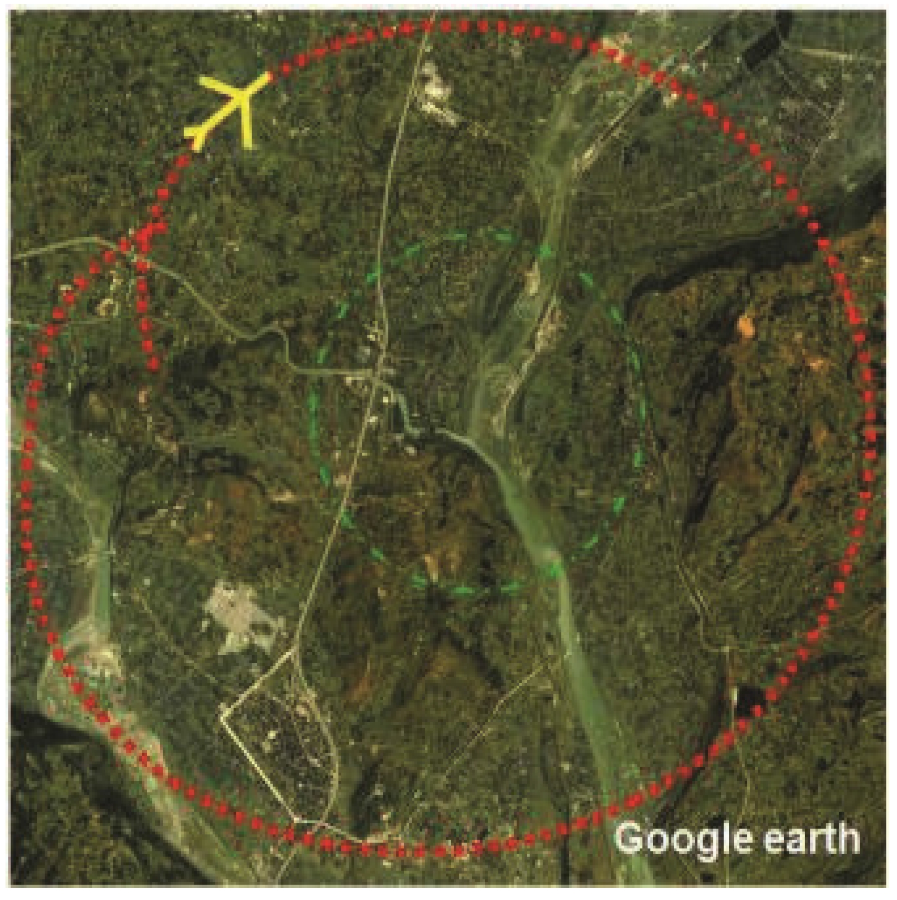
2.1. Dataset

The full polarimetric data is acquired over the suburban area of Sichuan, China, by the Institute of Electronics, Chinese Academy of Sciences with an airborne CSAR system at P-band. The imaging algorithm is back-projection algorithm [4]. Data is radiometric and phase calibrated. The experimental parameters are shown in

Table 1. Experimental parameters [4].

Polarization	HH HV VH VV
Carrier frequency	600 MHz
Bandwidth	200 MHz
Circle radius	≈3000 m
Mean height	≈3000 m

. The test area is shown in Figure 1. The experimental area has abundant man-made structures, such as buildings, bridges, highways, and an agricultural area with different crops. Both anisotropic and isotropic targets are easy to find in the experimental area.

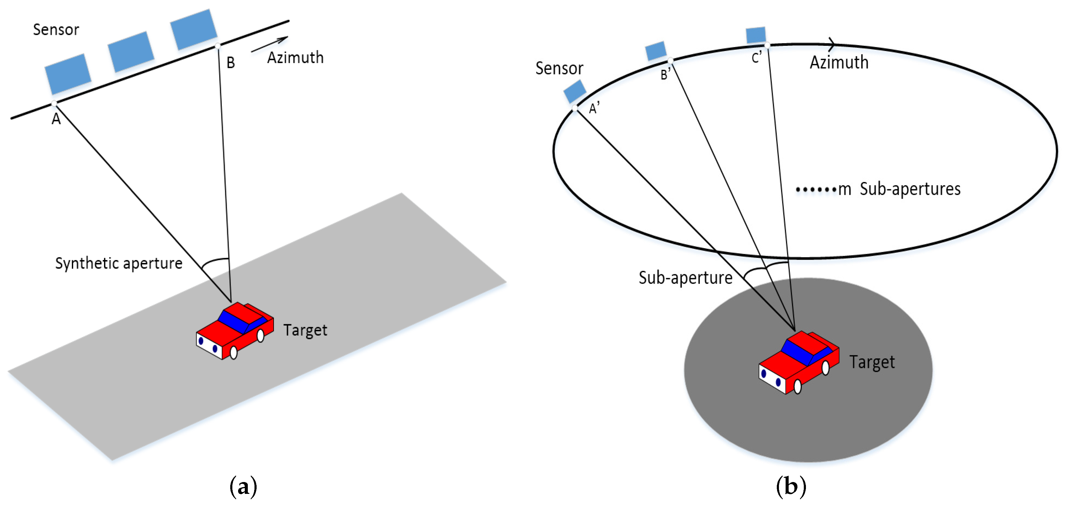
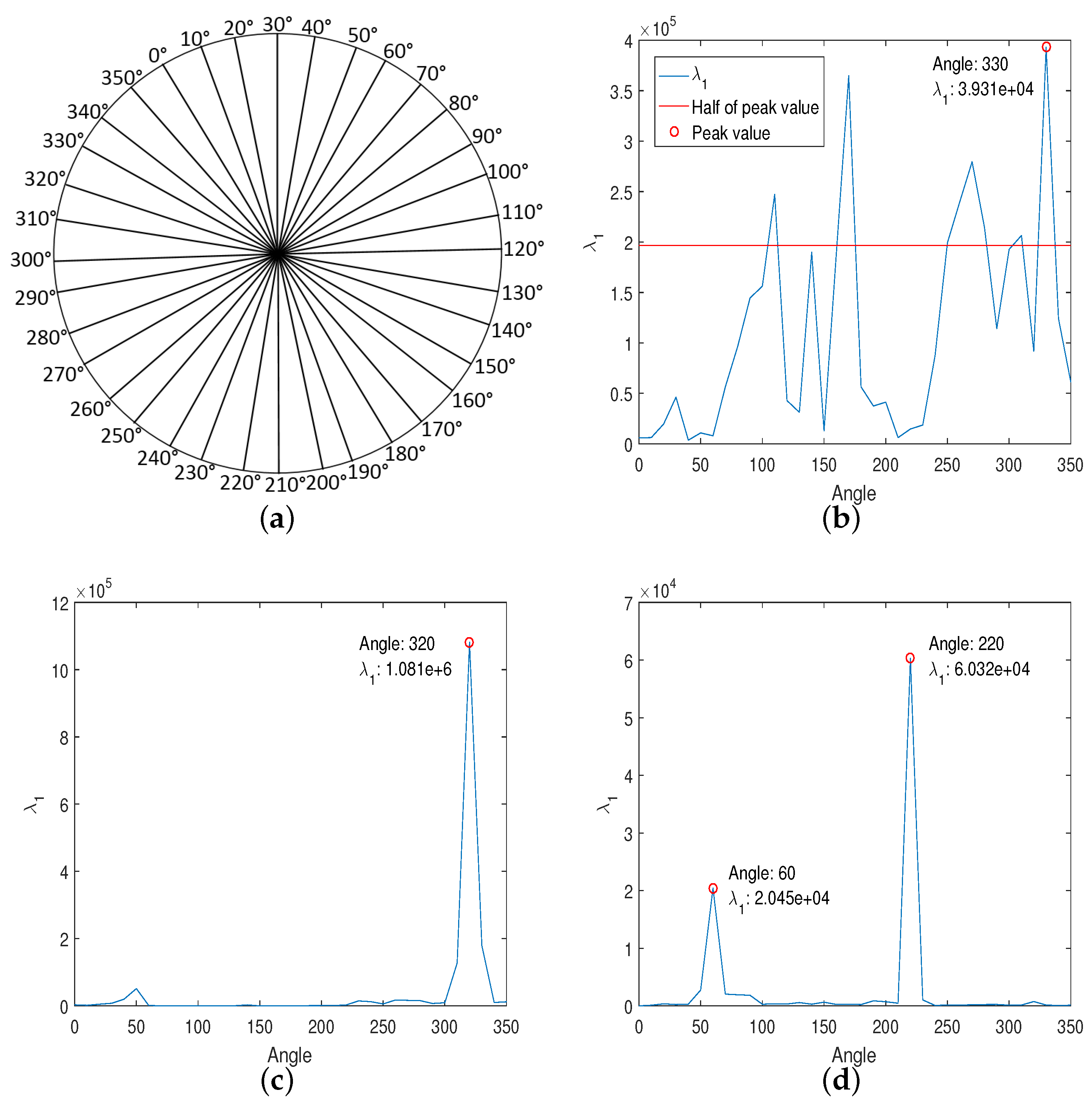
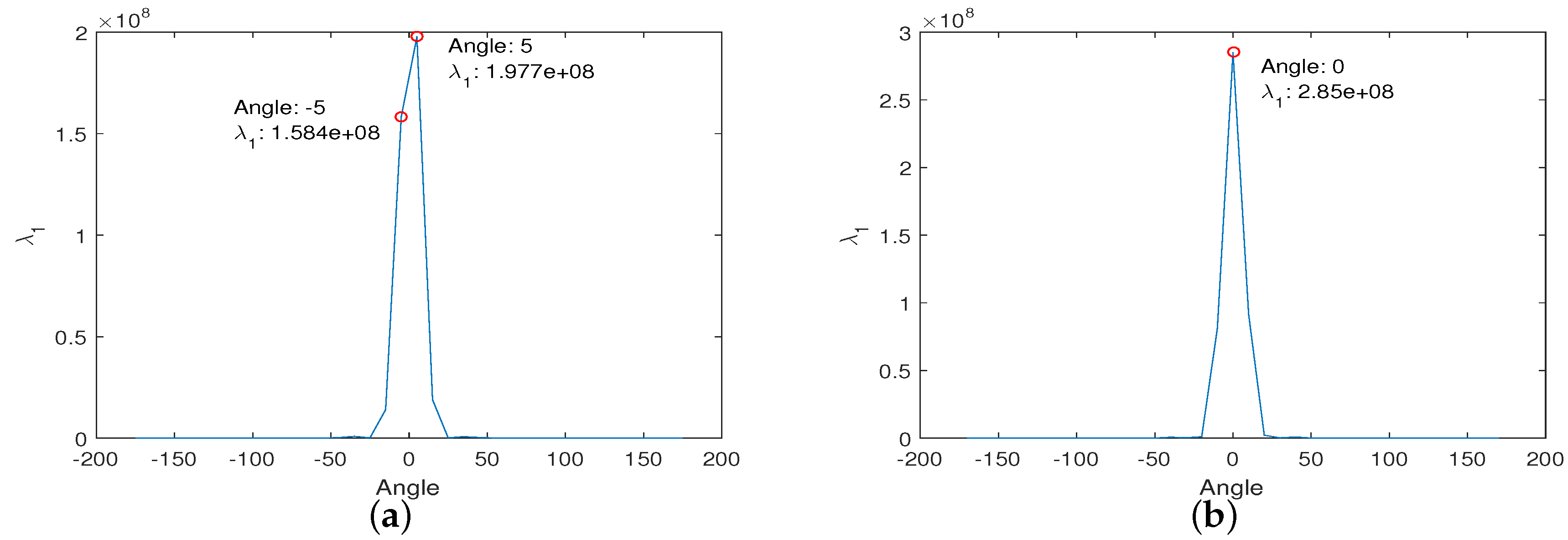
2.2. Multi-Aperture Observation Model

In traditional SAR polarimetry, the coherent scattering matrix $\mathit{S}$ contains full polarimetric information of illuminated targets

$$\begin{array}{c}\hfill \mathit{S}=\left[\begin{array}{c}{S}_{HH}{S}_{HV}\\ S_{VH}{S}_{VV}\end{array}\right],\end{array}$$

(1)

where H and V represent horizontal and vertical directions, respectively. $HH$, $HV$, $VH$, and $VV$ represent four linear orthogonal polarization combinations. Point-like scattering, defined as scattering from an isolated target which are smaller than resolution, is usually described with $\mathit{S}$ [20]. For the reciprocal backscattering case $S_{HV}=S_{VH}$, the target vector with Pauli base is defined as in [21]

$$\begin{array}{c}\hfill \mathit{k}=\frac{1}{\sqrt{2}}{[S_{HH}+S_{VV}{S}_{HH}-S_{VV}2S_{HV}]}^T,\end{array}$$

(2)

where the operator ${}^T$ denotes the transpose.

The traditional observation model only describes polarimetric information from a specific incidence angle. Figure 2a illuminates the traditional SAR observation model. The polarimetric properties observed at A and B are assumed invariant. The observed target vector $\mathit{k}$ is actually the coherent adding from A to B. Potential azimuthal variations are ignored during the formation of aperture. Meanwhile, whether a target has dominant scattering direction is a interesting question when aperture is large. Traditional observation model also can not describe the uncertainty of scattering direction. Figure 2b shows a target observed by Pol-CSAR with ${360}^{\circ }$ azimuthal aperture. Traditional observation model [3,22] can hardly describe information acquired by sensor from ${360}^{\circ }$. This paper proposes a multi-aperture observation model as shown in Figure 2b. Firstly, sensor is considered to observe m times during a circle. For example the first observation is from $A^{\prime }$ to $B^{\prime }$, and then from $B^{\prime }$ to $C^{\prime }$ the second observation is made, etc. Each observation has equal aperture. Therefore, ${360}^{\circ }$ aperture is cut into m sub-apertures, with an equal angle. From m sub-apertures, m target vectors are acquired. The multi-aperture observation model contains polarimetric information from m angles. Compared with the traditional observation model, polarimetric properties from different angles of view are accessible, variations are preserved and uncertainty of scattering direction can be described in the proposed model. In addition, although our model is illuminated with Pol-CSAR system, it can be applied to wide-angle SAR as well as traditional SAR.

The target vector for a multi-aperture situation is then defined as

$$\begin{array}{c}\hfill \mathit{p}={[{\mathit{k}}_1^T{\mathit{k}}_2^T\cdots {\mathit{k}}_{\mathrm{m}}^T]}^T,\end{array}$$

(3)

where $\mathit{p}$ has dimension $l=3\mathrm{m}$ and contains full polarimetric information from all angles of view. The $l\times l$ n-look multi-aperture coherency matrix $\mathit{D}$ is

$$\begin{array}{c}\hfill \mathit{D}=\frac{1}{n}\sum _{j=1}^n{\mathit{p}}_{\mathit{j}}·{\mathit{p}}_{\mathit{j}}^{T\ast }=\left[\begin{array}{c}{\mathit{T}}_{11}{\mathit{T}}_{12}\cdots {\mathit{T}}_{1\mathrm{m}}\\ {\mathit{T}}_{21}{\mathit{T}}_{22}\cdots {\mathit{T}}_{2\mathrm{m}}\\ ⋮\ddots ⋮\\ {\mathit{T}}_{\mathrm{m}1}\cdots {\mathit{T}}_{\mathrm{mm}}\end{array}\right],\end{array}$$

(4)

where the operator ${}^{\ast }$ denotes the complex conjugate , and ${\mathit{p}}_{\mathit{j}}$ is the multi-aperture target vector for the jth sample. n represents the sample number.The SAR signal is affected by speckle [23]. To avoid the effect of speckle, n is recommended to be larger than 49 ($7\times 7$ Boxcar filter) [24,25]. In the following experiment, n equals 81 ($9\times 9$ Boxcar filter). ${\mathit{T}}_{ii}$ is the sample coherency matrix of ith sub-apertures. Distributed scattering, from targets which are situated in a dynamically changing environment and are subject to spatial and temporal variations, is usually described with $\mathit{T}$ [20]. ${\mathit{T}}_{il}$ is the cross-correlation between the ith and lth sub-apertures. If the ith and lth sub-apertures do not overlap, then they do not have coherency and ${\mathit{T}}_{il}$ does not have useful information [26]. Dihedral is used as example to demonstrate the former declaration. In SAR polarimetry, $\mathit{S}$ of the horizontal dihedral is [20,27,28]

$$\begin{array}{c}\hfill {\mathit{S}}_{\mathit{dihedral}}=\left[\begin{array}{c}10\\ 0-1\end{array}\right],\end{array}$$

(5)

which means the phase difference between $HH$ and $VV$ is $\pi$. Figure 3 shows the phase difference of $H{H}_i$ and $V{V}_l$. More detailed information about the scene is provided in Section 3.2, and Figure 4a. In Figure 3a, two sub-apertures are at $0^{\circ }$–${120}^{\circ }$ and ${60}^{\circ }$–${180}^{\circ }$, with ${60}^{\circ }$ overlap. Buildings and trees have dihedral scattering [28] in the P band, which agrees with the values in Figure 3a. In Figure 3b, two sub-apertures are at $0^{\circ }$–${120}^{\circ }$ and ${120}^{\circ }$–${240}^{\circ }$ without overlap. There is no useful phase information in Figure 3b. Sub-apertures are chose to not overlap with each other in spectrum in the following experiment, so that all useful information is in diagonal items in (4) and off-diagonal items in (4) can be forced to zero.

Thus,

$$\begin{array}{c}\hfill {\mathit{T}}_{il}=\left\{\begin{array}{c}\frac{1}{n}\sum _{j=1}^n{\mathit{k}}_{ij}·{\mathit{k}}_{lj}^{T\ast }\mathrm{if}i=li,l\in (1\cdots \mathrm{m})\\ 0 \mathrm{if}i\ne li,l\in (1\cdots \mathrm{m})\end{array}\right.,\end{array}$$

(6)

where ${\mathit{k}}_{ij}$ is the target vector for the jth sample of ith sub-aperture. Using Equations (4) and (6), $\mathit{D}$ can be simplified to

$$\begin{array}{c}\hfill \mathit{D}=\left[\begin{array}{c}{\mathit{T}}_{11}0\cdots 0\\ 0{\mathit{T}}_{22}\cdots 0\\ ⋮\ddots ⋮\\ 0\cdots {\mathit{T}}_{\mathrm{mm}}\end{array}\right].\end{array}$$

(7)

$\mathit{D}$ contains full polarimetric information and is suitable for anisotropic anlysis.

2.3. Multi-Aperture Polarimetric Entropy

In the traditional observation model, polarimetric entropy only describes polarimetric randomness [19,29,30,31,32]. In the multi-aperture observation model, a parameter that can simultaneously describe polarimetric randomness and variations across sub-apertures is needed. Applying eigendecomposition to $\mathit{D}$

$$\begin{array}{cc}\mathit{D}\hfill & ={\mathit{U}}_D{\mathbf{\Sigma }}_D{\mathit{U}}_D^{-1}=\left[\begin{array}{c}{\mathit{U}}_{11}{\mathbf{\Sigma }}_{11}{\mathit{U}}_{11}^{-1}\\ {\mathit{U}}_{22}{\mathbf{\Sigma }}_{22}{\mathit{U}}_{22}^{-1}\\ \ddots \\ {\mathit{U}}_{\mathrm{mm}}{\mathbf{\Sigma }}_{\mathrm{mm}}{\mathit{U}}_{\mathrm{mm}}^{-1}\end{array}\right]\hfill \\ & =\sum _{k=1}^{3\mathrm{m}}{\lambda }_k{\mathit{u}}_k{\mathit{u}}_k^{T\ast }with{\mathit{T}}_{jj}={\mathit{U}}_{jj}{\mathbf{\Sigma }}_{jj}{\mathit{U}}_{jj}^{-1}j\in (1\cdots \mathrm{m}),\hfill \end{array}$$

(8)

where $\mathit{U}$ is composed of eigenvectors, $\mathit{u}$; $\mathbf{\Sigma }$ is composed of eigenvalues, $\lambda$; and the eigenvalues of $\mathit{D}$ are the same as the eigenvalues of each sub-aperture. MAPE is defined as

$$\begin{array}{c}\hfill \begin{array}{c}\hfill H_{\mathrm{multi}}=-\sum _{k=1}^{3\mathrm{m}}{P}_k{\log }_{3m}\left(P_k\right)\\ \hfill with{P}_k=\frac{{\lambda }_k}{{\sum }_{i=1}^{3\mathrm{m}}{\lambda }_i}.\end{array}\end{array}$$

(9)

In this paper, MAPE is suggested as an extension of polarimetric entropy in multi-aperture situation. Since polarimetric entropy describes the uncertainty of scattering process, MAPE, due to the combination of polarimetric and azimuthal information, can describe both uncertainty of scattering process and scattering direction. MAPE has three properties.

Property 1.

When MAPE is lower, targets have high certainty both in scattering process and direction, which means targets are weakly depolarized and there is/are dominant sub-aperture(s) with stronger scattering because small MAPE refers to

$$\begin{array}{c}\hfill {\lambda }_i\gg {\lambda }_{l}l\in (1,\cdots ,i-1,i+1,\cdots ,\mathrm{m}),\end{array}$$

(10)

which indicates that there is an eigenvalue larger than the others. Therefore, targets with small MAPE have certain direction and scattering mechanism, thus are considered as anisotropic. Dihedrals, for example, have strong scattering when the sensor is facing them directly. As the angle of view changes, the power of received echoes decreases. The quadratic sum of eigenvalues is proportional to echo power [33]. Thus eigenvalues of the straight view sub-aperture are larger than others, which results in small MAPE.

Property 2.

When MAPE is higher, targets have high uncertainty both in scattering process and direction, which means targets are strongly depolarized and there is no dominant sub-aperture.

$$\begin{array}{c}\hfill {\lambda }_i\approx {\lambda }_{l}i,l\in (1,\cdots ,\mathrm{m}),\end{array}$$

(11)

which indicates small eigenvalue variations. The coherency matrices of all sub-apertures are strongly depolarized and no sub-aperture is dominant. Since the quadratic sum of eigenvalues is proportional to echo power, echo power is almost constant for each sub-aperture. This represents random scatter with no polarization dependence.

Property 3.

When MAPE is in the middle, targets have high uncertainty in scattering direction but moderate uncertainty in scattering process, which means targets are weakly depolarized and there is no dominant sub-aperture. Eigenvalues in each sub-aperture are

$$\begin{array}{c}\hfill {\mathit{T}}_{ii}={\mathit{U}}_{ii}{\mathbf{\Sigma }}_{ii}{\mathit{U}}_{ii}^{-1}=\sum _{k=1}^3{\lambda }_k{\mathit{u}}_k{\mathit{u}}_k^{T\ast }.\end{array}$$

(12)

Firstly, within a sub-aperture, the eigenvalues is sorted with ${\lambda }_1\ge {\lambda }_2\ge {\lambda }_3$. The situation that targets are weakly depolarized is referred to in [19] as

$$\begin{array}{c}\hfill {\lambda }_1\gg {\lambda }_2\approx {\lambda }_3\approx 0.\end{array}$$

(13)

Then, with no dominant sub-aperture

$$\begin{array}{c}\hfill {\lambda }_{1i}\approx {\lambda }_{1l}i,l\in (1\cdots \mathrm{m}),\end{array}$$

(14)

${\lambda }_{1i}$ is the biggest eigenvalue of the ith sub-aperture and ${\lambda }_{1l}$ is the biggest eigenvalue of the lth sub-aperture. Tophat , for example, has same dihedral scattering mechanism in every sub-aperture, conforms to Equations (13) and (14), and has moderate MAPE.

The three properties can be used to identify anisotropic and isotropic targets. However, limited by speckle [34,35], theoretic thresholds to determine whether MAPE is high, low or moderate are hard to acquire. Instead, experiential thresholds are used in this paper. Targets with MAPE of less than 0.55 are anisotropic; targets with MAPE more than 0.55 and less than 0.7 are isotropic; and targets with MAPE greater than 0.7 have random scatter with no polarization dependence.

Comparing MAPE with polarimetric entropy, values for isotropic targets are different. We consider the ideal model that scattering from all sub-apertures is the same, which indicates same coherency matrices

$$\begin{array}{c}\hfill {\mathit{T}}_{ll}={\mathit{T}}_{ii}l,i\in (1\cdots \mathrm{m}).\end{array}$$

(15)

For each sub-aperture, the polarimetric entropy is [19]

$$\begin{array}{c}\hfill \begin{array}{c}\hfill H=-\sum _{k=1}^3{P}_k{\log }_3\left(P_k\right)\\ \hfill with{P}_k=\frac{{\lambda }_k}{{\sum }_{i=1}^3{\lambda }_i}.\end{array}\end{array}$$

(16)

From Equations (9), (15) and (16), the difference between MAPE and polarimetric entropy is

$$\begin{array}{c}\hfill {\delta }_H=H-H_{multi}=(1-H){\log }_{3\mathrm{m}}\mathrm{m}\le 0,\end{array}$$

(17)

which suggests that MAPE values are larger than polarimetric entropy for isotropic targets, due separate with a threshold. Thus to the lack of directivity. The MAPE of isotropic targets and random scatters is usually difficult to separate with a threshold, thus Equation (17) is used to identify isotropic targets together with MAPE in the following experiment.

3. Results and Discussion

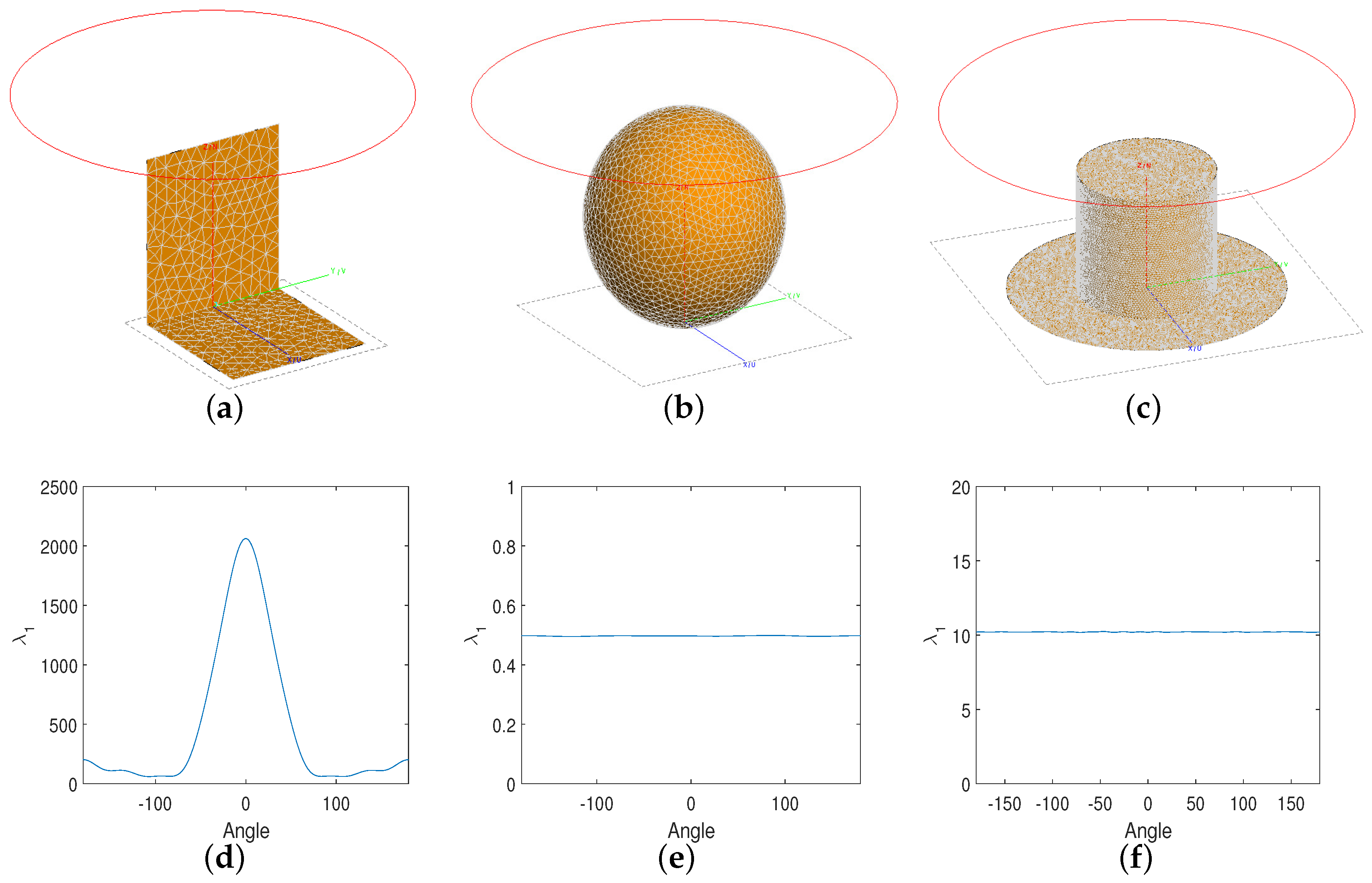
3.1. Simulation

Point-like scattering, from targets which are smaller than the radar footprint and distributed scattering, from targets which are situated in a dynamically changing environment and are subject to spatial and temporal variations.

Typical point targets are simulated by Feko 7.0 to demonstrate the former properties. Dihedrals are anisotropic, while spheres and tophats are isotropic. Dihedrals are made up with two squares. The sides of squares are 2 m in length. Two squares are perpendicular to each other. The radius of the sphere measures 1 m. The tophat is made up with a cylinder and a circular plate. The radius of plate is 1 m. The radius of cylinder is 0.5 m and the height of cylinder is 1 m. The frequency of the plane wave is 600 MHz. The variations of ${\lambda }_1$ across angles of view are shown in Figure 5d–f. ${\lambda }_1$ of the dihedral has the largest value when the sensor is facing it directly. Then, ${\lambda }_1$ rapidly decreases to 0 when the angle of view changes from $0^{\circ }$ to ${90}^{\circ }$. ${\lambda }_1$ of the sphere and tophat stay invariant in different angles of view. ${\lambda }_2$ and ${\lambda }_3$ of the dihedral, sphere, and tophat are approximately 0 because of the low polarimetric randomness.

Table 2. Multi-aperture polarimetric entropy (MAPE) and the polarimetric entropy of typical targets.

Targets	Entropy	MAPE
Dihedral	≈0	0.2189
Sphere	≈0	0.66
Tophat	≈0	0.6584
River surface target	0.814	0.753

shows MAPE and entropy of typical targets. The multi-look data is simulated by Lee’s method [36]. The scattering vector with a linear base is [21]

$$\begin{array}{c}\hfill \mathit{u}={\left[S_{HH}\frac{\sqrt{2}}{2}(S_{HV}+S_{VH})S_{HV}\right]}^T,\end{array}$$

(18)

and the covariance matrix is [21]

$$\begin{array}{c}\hfill \mathit{C}=E\left[\mathit{u}{\mathit{u}}^{\ast T}\right],\end{array}$$

(19)

where E represents expectation. The main steps of the simulation are [36]:

• For a given $\mathit{C}$, calculate ${\mathit{C}}^{\frac{1}{2}}$ with

  $$\begin{array}{c}\hfill {\mathit{C}}^{\frac{1}{2}}{({\mathit{C}}^{\frac{1}{2}})}^{\ast T}=\mathit{C},\end{array}$$

  (20)
• Simulate a complex random vector $v$, which obeys complex normal distribution with mean zero, and the covariance matrix equals the identity matrix. The real and imaginary part of each complex element of $v$ are normally distributed with mean zero and variance $\frac{1}{2}$.
• Compute the 1-look complex scattering vector

  $$\begin{array}{c}\hfill \mathit{u}={\mathit{C}}^{\frac{1}{2}}\mathit{v}.\end{array}$$

  (21)
• Calculate the n-look covariance matrix

  $$\begin{array}{c}\hfill {\mathit{C}}_{\mathit{n}}=\frac{1}{n}\sum _1^n\mathit{u}{\mathit{u}}^{\ast T}.\end{array}$$

  (22)

The full polarimetric data of the river surface are real Pol-CSAR data (see more detailed information in Section 3.2). The entropy of the dihedral is calculated with polarimetric data from a directly facing angle. Since tophat and sphere are isotropic targets, the entropy is calculated with polarimetric data from the same direction as the dihedral. The entropy of the river surface is calculated using sub-aperture $0^{\circ }$–${30}^{\circ }$ data with $9\times 9$ multi-look. The result in Table 2 agrees with the formal discussion. The dihedral has low MAPE, the sphere and tophat have moderate MAPE, and the river surface has high MAPE. In addition, sphere and tophat satisfy (17). Sphere and tophat can be easily distinguished from the river surface by (17). Notice that the tophat has dihedral scattering in each direction, which is hard to distinguish with dihedral using entropy. However, dihedral and tophat are easy to distinguish using MAPE.

3.2. Real Data

In this paper, two areas in Figure 1 are selected. The first area mainly contains a power station and some buildings and is used to test the MAPE’s ability for identifying anisotropic and isotropic targets. The second area is an agricultural area, which contains different isotropic targets and is used to test MAPE’s ability of distinguishing isotropic targets which have different polarimetric randomness.

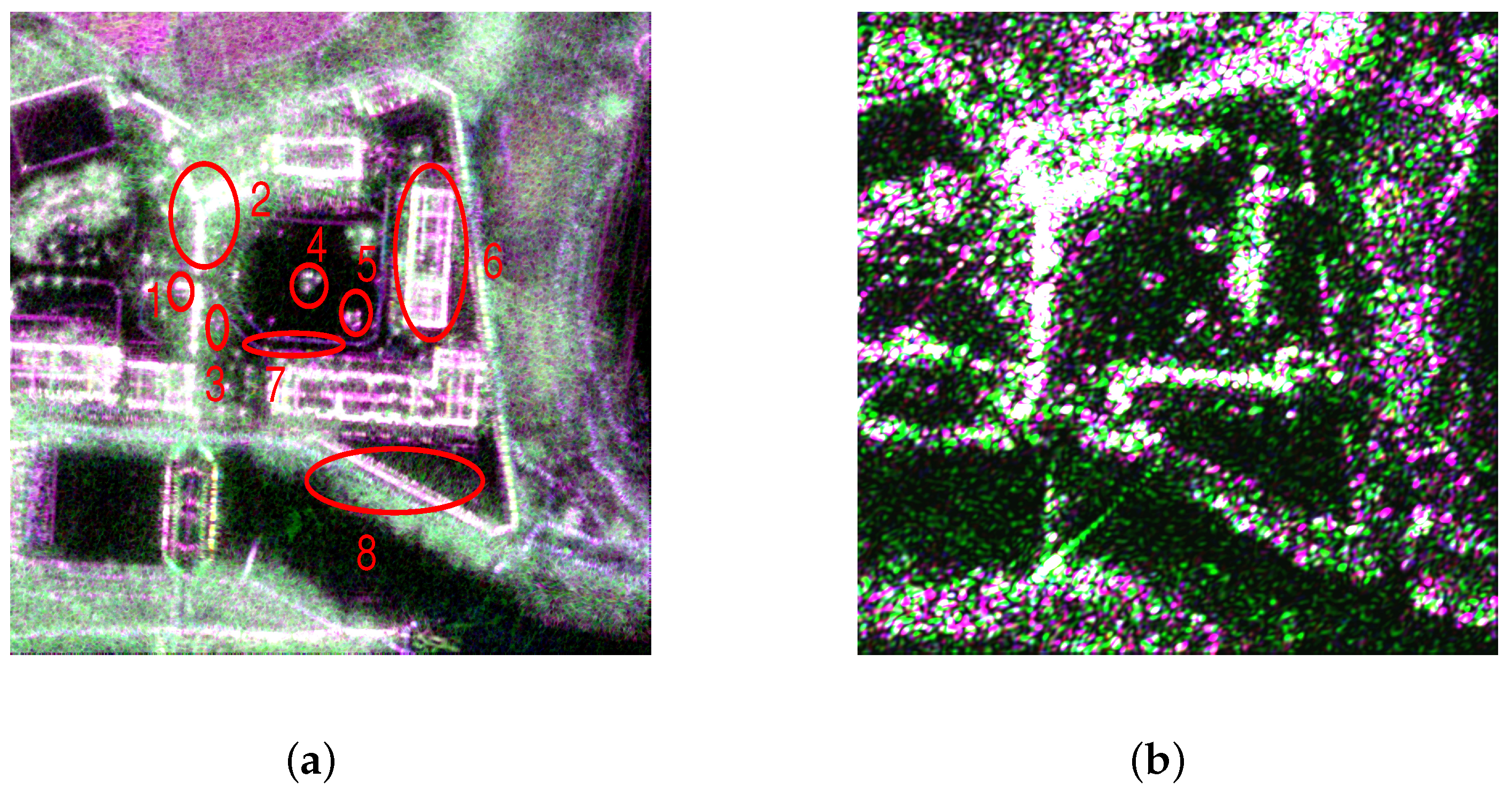
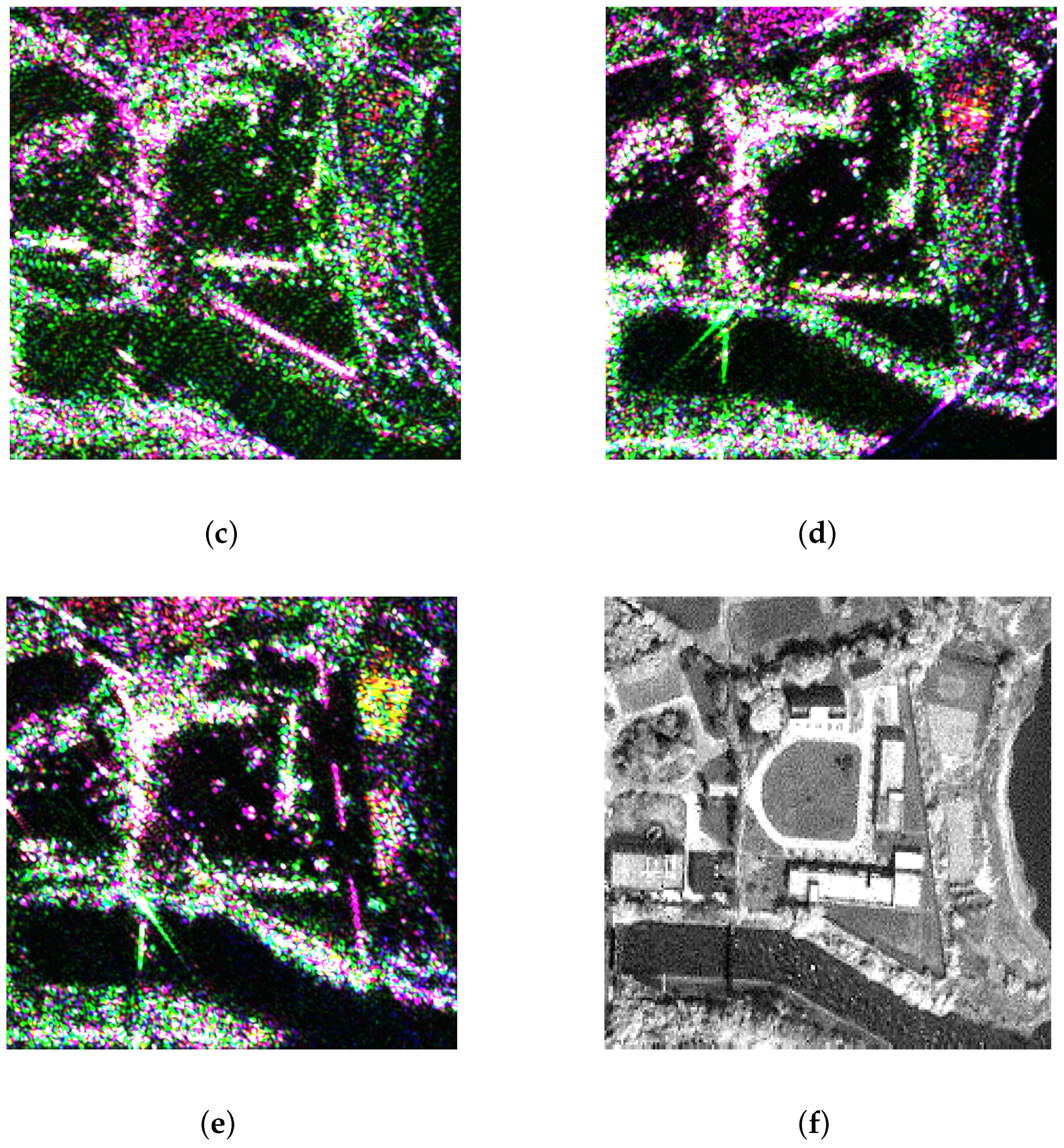
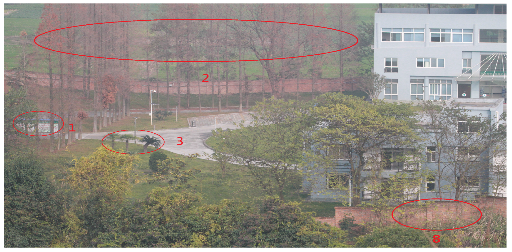
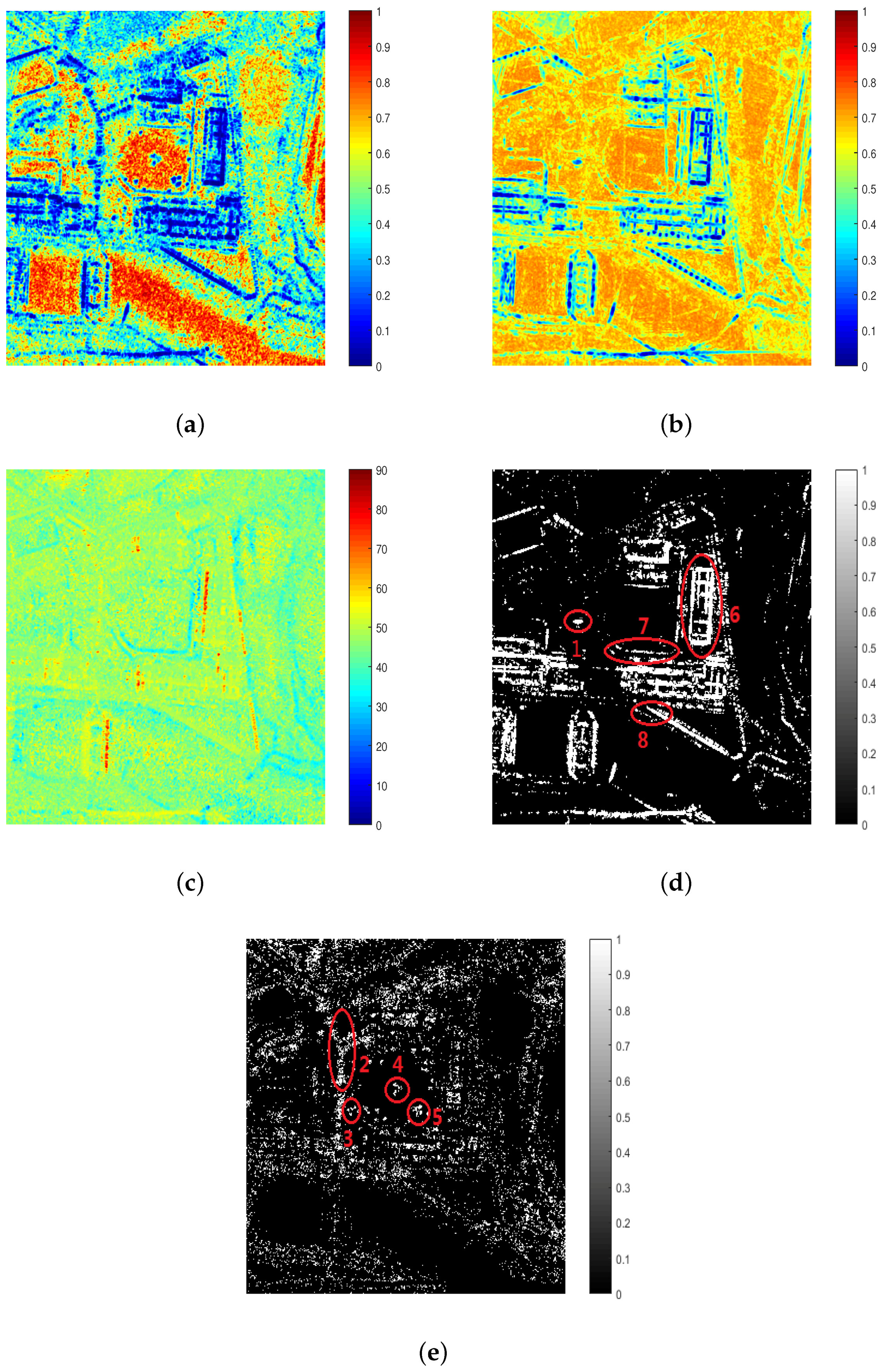
3.2.1. Power Station and Buildings

Figure 4a,f show polarimetric and optical images, respectively, of a power station and buildings. Figure 4a is formed by ${360}^{\circ }$ coherent azimuthal integration of Pol-CSAR data. The viewed area contains many artificial and natural targets, with eight particular targets marked in Figure 4a. Target 1 is a billboard, target 2 is some tall trees in the shape of capital Y, and target 3 marks three short trees. Targets 4 and 5 are similar to target 3. Target 6 is a building, and target 7 is footpath in the shape of pentagon . Target 8 is a brick wall. Targets 1–3 and 8 are also shown visually in Figure 6. Figure 4b is a $0^{\circ }$–${10}^{\circ }$ sub-aperture image, Figure 4c is a ${90}^{\circ }$–${100}^{\circ }$ sub-aperture image, Figure 4d is a ${180}^{\circ }$–${190}^{\circ }$ sub-aperture image and Figure 4e is a ${270}^{\circ }$–${280}^{\circ }$ sub-aperture image. Only parts of the buildings, bridges, and walls are in Figure 4b–e because anisotropic targets have changing scattering properties and cannot be seen in all angles of view. On the other hand, isotropic targets, e.g., trees and lamps, exist in Figure 4b–e. CSAR, with large azimuthal aperture, can more precisely and completely describe targets and provide enough information to distinguish anisotropic and isotropic targets.

The Pol-CSAR data is separated into $36\times {10}^{\circ }$ sub-apertures in the following experiment. Sub-apertures do not overlap with each other in spectrum. Figure 7a shows the direction of each sub-aperture. The variations of ${\lambda }_1$ across sub-apertures of targets 2, 6, and 7 are shown in Figure 7b–d. Target 2 is similar to tophat since electromagnetic wave at P band has strong penetration. In Figure 7b, ${\lambda }_1$ of six sub-apertures are above half of the maximum ${\lambda }_1$. MAPE is 0.6707. Variations of ${\lambda }_1$ across sub-apertures are mainly caused by interaction between the trees, since the distance between trees is less than 1 m. The wall of target 6 forms a dihedral shape with the ground. The curve of ${\lambda }_1$ in Figure 7c is a similar curve that in Figure 5d. The peak of curve in Figure 7c is located at ${320}^{\circ }$, when the sensor is facing target 6 directly. The MAPE is 0.3142. Target 7 has strong surface scattering when the angle of view is vertical to it (theoretically ${40}^{\circ }$ and ${220}^{\circ }$ in Figure 7a). In Figure 7d, ${\lambda }_1$ is the largest and is the second-largest at ${60}^{\circ }$ and ${220}^{\circ }$. The MAPE is 0.3259. The results of the experiment with real data agree with the simulation. Target 2 contains lots of trees, while in simulation only isolated tophat is illuminated by sensor. The ${\lambda }_1$ of target 2 does not stay invariant across sub-aperture due to the effect of other trees. Still, target 2 is identified as an isotropic target and targets 6 and 7 are identified as anisotropic targets by the MAPE.

Figure 8a shows the polarimetric entropy of Figure 4a calculated by (16). Figure 8b shows MAPE calculated by (9). Figure 8c shows $\alpha$ of the experimental scene(detailed method to calculate $\alpha$ is in [19]). Since MAPE is suggested as an extension of polarimetric entropy in multi-aperture situation, polarimetric entropy and MAPE (Figure 8a,b) are compared. Firstly, the brick wall (target 8) is continuous in Figure 8a, while alternating in Figure 8b because of a two-trihedral special structure. Figure 6 shows the details of the brick wall. This special structure is more anisotropic than a flat wall. Thus, the MAPE in these areas is much smaller than in the rest of the wall. Secondly, trees in the shape of capital Y (target 2), lamps, and shorter trees have low values in Figure 8a but high values in Figure 8b which agrees with (17). Trees and billboard are hard to distinguish in Figure 8a, but distinct in Figure 8b, which shows MAPE’s ability to distinguish anisotropic and isotropic targets since the billboard is an anisotropic target.

Figure 8d shows anisotropic targets identified by MAPE. The billboards are well identified. The footpath, which has surface scattering, and buildings, which have dihedral scattering when vertical to the radar angle of view, are also identified. Brick walls, although affected by vegetation areas, are also identified. Figure 8e shows isotropic targets identified using (17). Trees have dihedral and volume scattering in all sub-apertures, and hence are all well identified as isotropic targets [28]. Some vegetation areas toward the top and bottom of the image, though have higher randomness, are also considered as isotropic targets. Result demonstrates that MAPE can distinguish anisotropic and isotropic targets. Since most anisotropic targets are man-made targets, MAPE can be applied for man-made target detection.

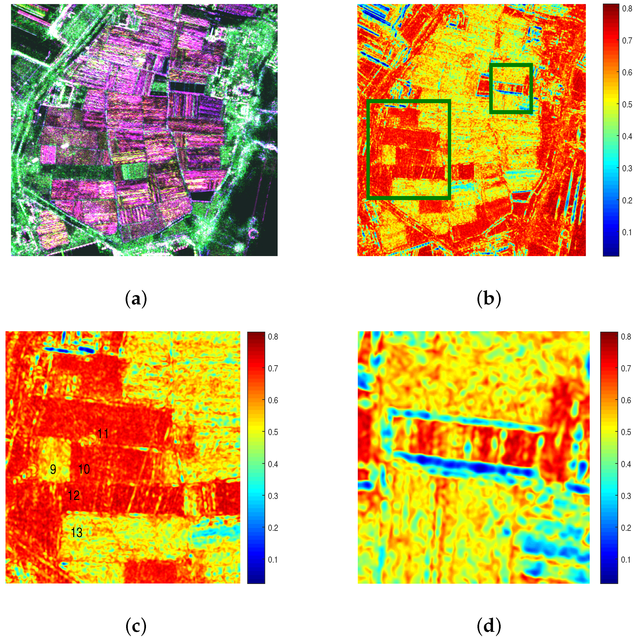
3.2.2. Agricultural Area

Figure 9a is image of farmland and is formed by ${360}^{\circ }$ coherent azimuthal integration of Pol-CSAR data. Figure 9b is MAPE. Figure 9c,d show enlarged images of the two rectangles in Figure 9b. There are five targets in Figure 9c. Targets 9, 10, 12, and 13 are four pieces of farmland. Target 11 marks two telegraph poles. Targets 9 and 13 are planted with same crops. Target 10 grows some grass. Target 12 grows grass and some shrubs.

• In agricultural areas, farmland is planted with different crops that have different polarimetric randomness. Thus, targets 9 and 13 are significantly different from target 10 in Figure 9c.
• Targets 10 and 12 are slightly different. The difference between target 10 and 12 in Figure 9c is caused by shrubs.
• The two telegraph poles are different from target 10 in Figure 9c, although poles and target 10 are both isotropic. The difference between target 10 and poles is caused by different polarimetric randomness.

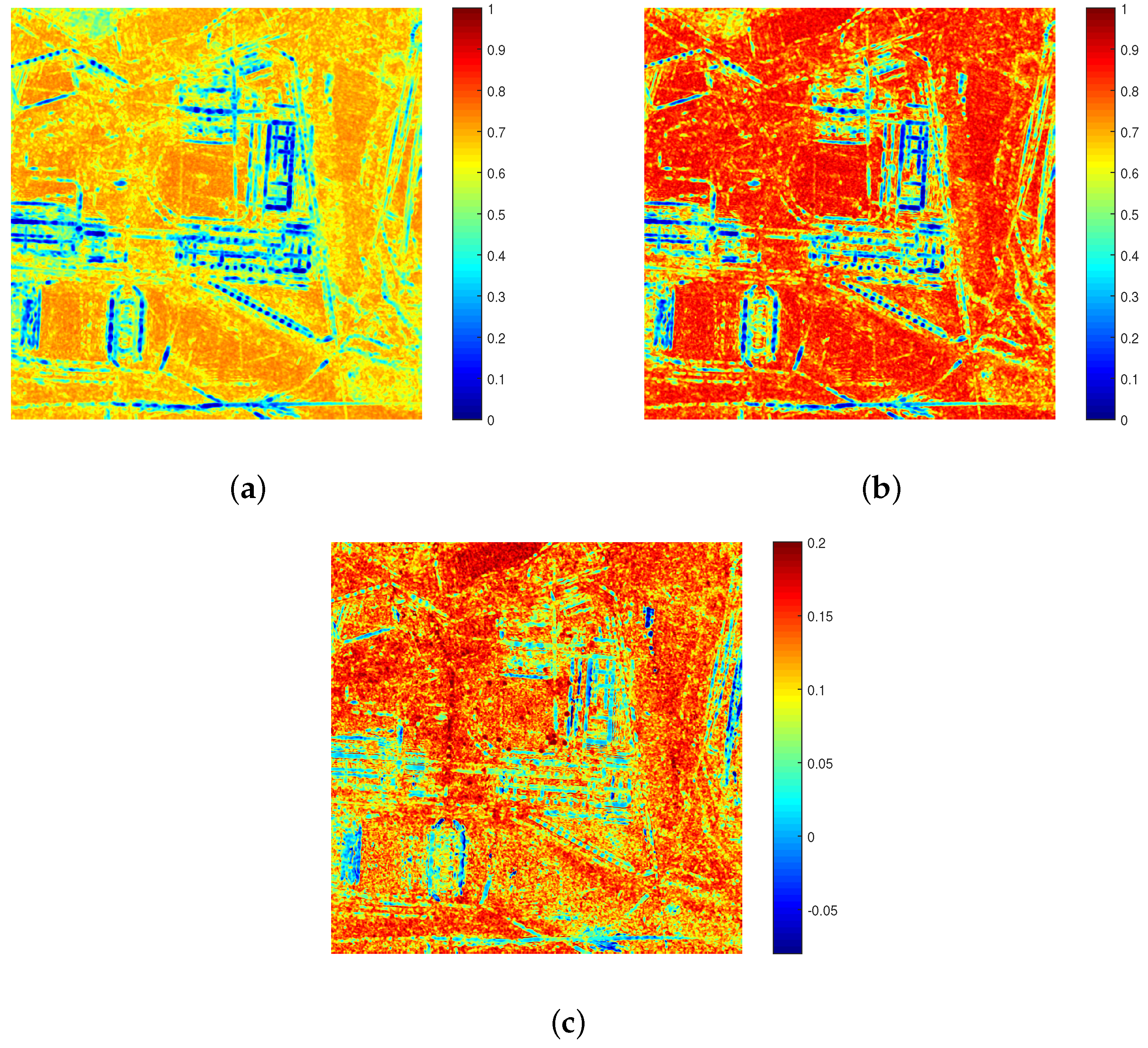
The differences among target 9, 10, and 13 show that MAPE has potential in farmland classification. The difference between target 11 and target 10 shows that MAPE can be applied to telegraph pole detection in agricultural areas.

Figure 9d shows a piece of farmland with Bragg resonances. Bragg resonances are due to the coherent summation of simultaneously constructive contributions from a set of scatterers [14]. Bragg scattering brings difficulties to farmland segmentation and classification. Bragg resonances are identified by MAPE as anisotropic scattering.

3.2.3. Comparison

Figure 10a shows MAPE, the same as in Figure 8b. Figure 10b shows directivity $\mathrm{\Lambda }$ presented by Xu in [18]. $\mathrm{\Lambda }$ describes the targets’ scattering directivity. In Figure 10b, $\mathrm{\Lambda }$ is transfered with $\mathrm{\Lambda }=1-\mathrm{\Lambda }$ for better comparison. $\mathrm{\Lambda }=0$ implies an impulse function, i.e., all energy directed toward one look angle, which corresponds to anisotropic targets, and $\mathrm{\Lambda }=1$ indicates equal energy to all look angles, which corresponds to isotropic targets [18]. Figure 10c shows the difference between MAPE and $\mathrm{\Lambda }$. The differences of MAPE and $\mathrm{\Lambda }$ for anisotropic targets are very small in Figure 10c, and equal approximately zero. As to isotropic targets, the differences of MAPE and $\mathrm{\Lambda }$ are much larger, approximately equaling 1.8. The difference is because that MAPE can describe the targets’ polarimetric randomness and variations, while $\mathrm{\Lambda }$ only describes variations. MAPE is the entropy of all sub-apertures’ eigenvalues. The variations of anisotropic targets’ eigenvalues across sub-apertures are much larger than within sub-aperture. Thus, the MAPE and $\mathrm{\Lambda }$ of anisotropic targets are very close. As to isotropic targets, variations across sub-apertures are very small (taking noise into consideration). Thus, isotropic targets’ $\mathrm{\Lambda }$ values are close to 1. Meanwhile, eigenvalues within each sub-aperture are not the same. Thus isotropic targets’ MAPE values are lower than 1. In fact, analysis using ideal model and simulation of isotropic targets suggests that isotropic targets’ MAPE values equal approximately 6.7. Thus, isotropic targets’ MAPE and $\mathrm{\Lambda }$ have large differences.

3.3. Discussion of Sub-Aperture Partition

In the former experiment, the size of sub-aperture is ${10}^{\circ }$ and the first sub-aperture starts from $0^{\circ }$. The effects of different size and start position of sub-apertures remain unconsidered. In this section, simulated data of dihedral is used to analyze these problems. The azimuth range of simulated data is from $-{180}^{\circ }$ to ${180}^{\circ }$. Firstly, 20 experiments are carried out. The start angles of each experiment are $-{180}^{\circ }$. The sizes of sub-apertures are from $1^{\circ }$ to ${20}^{\circ }$ with $1^{\circ }$ increment.

Table 3. MAPE of the dihedral with different sizes of sub-aperture.

Sub-aperture size	$1^{\circ }$	$2^{\circ }$	$3^{\circ }$	$4^{\circ }$	$5^{\circ }$	$6^{\circ }$	$7^{\circ }$	$8^{\circ }$	$9^{\circ }$	${10}^{\circ }$
MAPE	0.482	0.424	0.371	0.350	0.319	0.294	0.294	0.250	0.234	0.230
Sub-aperture size	${11}^{\circ }$	${12}^{\circ }$	${13}^{\circ }$	${14}^{\circ }$	${15}^{\circ }$	${16}^{\circ }$	${17}^{\circ }$	${18}^{\circ }$	${19}^{\circ }$	${20}^{\circ }$
MAPE	0.203	0.191	0.178	0.179	0.180	0.118	0.086	0.171	0.043	0.179

shows the MAPE of each experiment. MAPE decreases as the size of sub-aperture increases to ${14}^{\circ }$. The limiting value of MAPE is 0.179. The MAPE of ${16}^{\circ }$, ${17}^{\circ }$, and ${19}^{\circ }$ is caused by wrong start position of sub-apertures, which will be discussed in the following experiment. There is strong dihedral scattering from $-{30}^{\circ }$ to ${30}^{\circ }$. When the size of sub-apertures increases, the number of sub-apertures which observe strong scattering decreases. Consequently, dihedral is considered as more anisotropic and MAPE decreases. However, the simulation only contains one target. If there is more than one target and the scattering mechanism of each target is different, the scattering properties would more likely be averaged when the size of sub-aperture becomes larger. Experiential maximum sub-aperture size is ${10}^{\circ }$ to avoid mixed scattering properties. Meanwhile, if the sub-apertures are too small, the resolution becomes too small and images would be heavily affected by speckle. Thus, ${10}^{\circ }$ is the recommended sub-aperture size in this paper.

The start position of sub-aperture also affects the interpretation of the target scattering mechanism. In Figure 11, curves of ${\lambda }_1$ with different sub-aperture start position are compared. When the start position is $-{175}^{\circ }$, the range of the 18th sub-aperture is $-5^{\circ }$ to $5^{\circ }$. Consequently, there is only one peak value in Figure 11b. The MAPE is 0.2162. When the start position is $-{180}^{\circ }$, the ranges of the 18th and 19th sub-apertures are $-{10}^{\circ }$ to $0^{\circ }$ and $0^{\circ }$ to ${10}^{\circ }$, respectively. Thus, the 18th and 19th sub-apertures have high ${\lambda }_1$, as shown in Figure 11a. The curve is different in Figure 11b, and MAPE changes slightly to 0.2204. The choice of the sub-aperture’s start position is a target-wise problem and needs to be studied in future work.

4. Potential Application

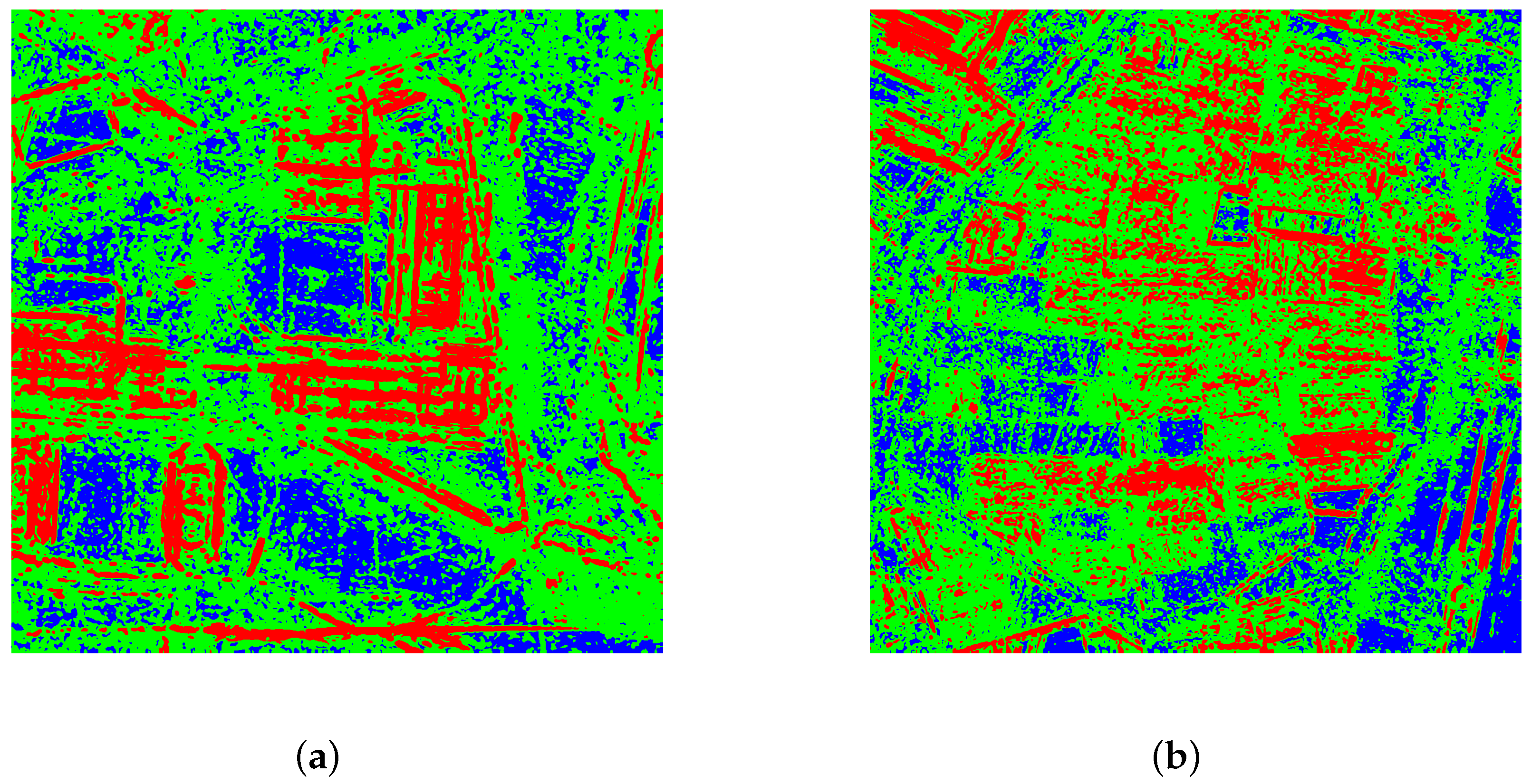
4.1. Classification

Polarimetric classification is a important field in SAR polarimetry. Many algorithms have been developed to classify natural media, especially in the field of agriculture [8,9,19,21,29,31,36]. However, as shown in Figure 9d, the agricultural area can be heavily affected by anisotropic Bragg scattering. The original scattering mechanisms can be covered by Bragg scattering and consequently the classification accuracy will be affected. Meanwhile, the traditional classification algorithm, limited by the observation model, can not distinguish anisotropic and isotropic targets. To solve this problem, Bragg scattering can be identified by MAPE and removed with the method in [14] before classification. Moreover, since anisotropy is an important part of targets’ scattering mechanisms, data can be firstly classified by MAPE. Then, anisotropic targets and isotropic targets are classified separately.

Figure 12 shows the classification result. Images are classified into three classes: anisotropic, isotropic, and random scatters. In Figure 12a, man-made targets, natural targets, and random scatters are separated. In Figure 12b, Bragg scattering and random scatters are separated with farmland. The result can be applied as initial classes to existing classification algorithms to achieve more precise classification.

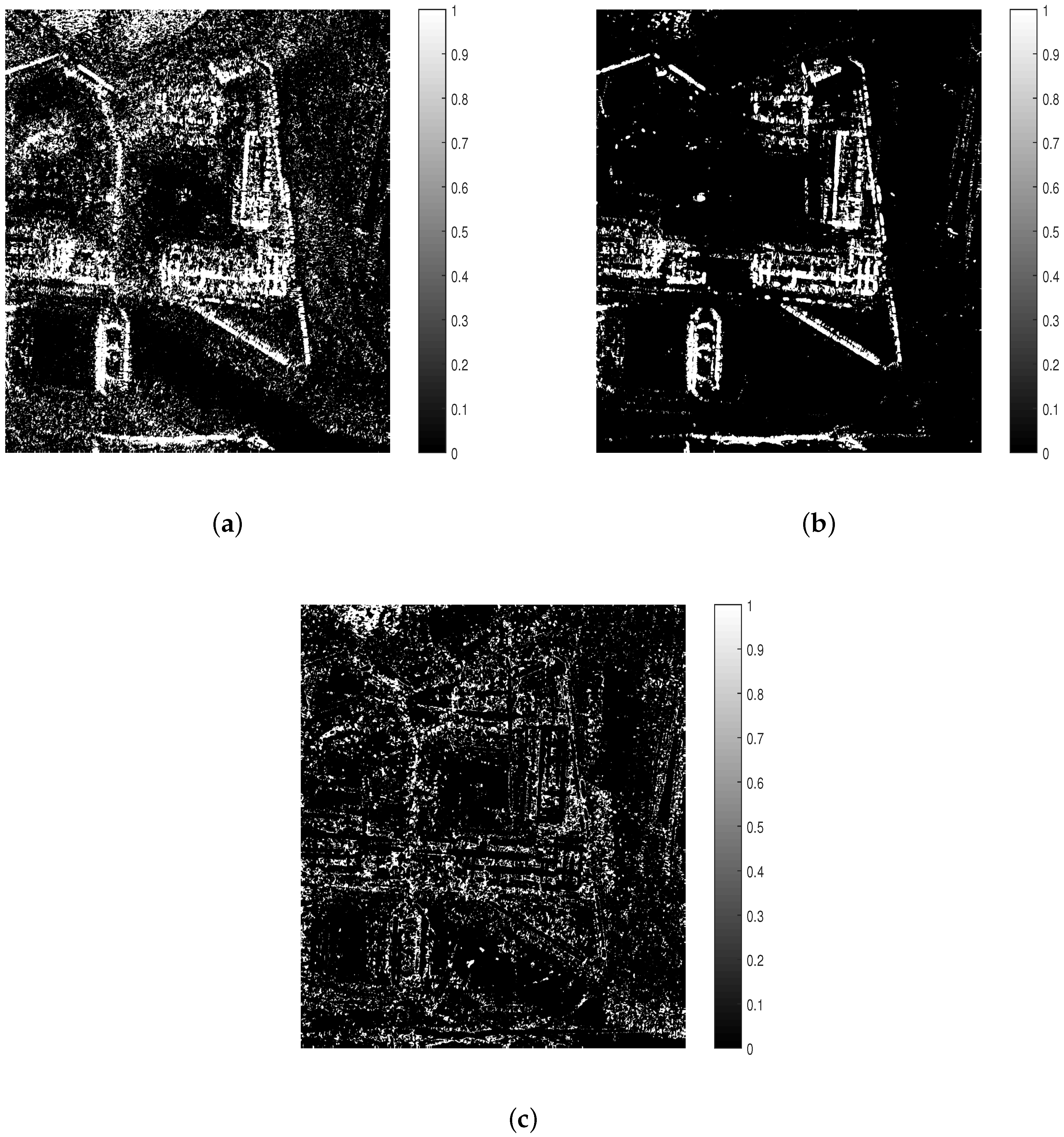
4.2. Target Discrimination

Polarimetric SAR data reflects targets’ scattering mechanisms and physical parameters such as material and shape. With polarimetric target decomposition theorems, the polarimetric matrix can be decomposed into several canonical scattering mechanisms [6]. For example, Freeman decomposition [28] uses dihedral, Bragg, and volume scattering as basic scattering mechanisms and can determine the dominant scattering mechanisms of observed backscatter; H-$\alpha$ decomposition uses entropy to measure the degree of scattering randomness and average $\alpha$ to determine dominant scattering mechanisms [19]. The polarimetric target decomposition theorems are widely used in target discrimination. However, the traditional method can not discriminate anisotropic targets with isotropic targets. Thus, man-made targets and natural targets may be mixed up by traditional method. The proposed MAPE, with the ability to identify anisotropic and isotropic targets, can improve the result of target discrimination.

Figure 13 shows targets discriminated by H-$\alpha$ and MAPE-$\alpha$. In Figure 13a, trees, buildings and the bridge are identified as having dihedral scattering by H-$\alpha$. H-$\alpha$ cannot discriminate trees with buildings and bridges. Buildings, walls, and the bridge are identified in Figure 13b as anisotropic dihedral scattering, while trees are identified in Figure 13c as isotropic dihedral scattering by MAPE and $\alpha$, respectively. The result shows that MAPE has improved the result of target discrimination. Consequently, man-made targets such as buildings and bridges as well as natural targets can be better identified.

5. Conclusions

In this paper, a multi-aperture observation model was proposed by considering the observation as a sequence of dispersed observation. Polarimetric data is then consequently separated into sub-apertures. The multi-aperture observation model contained polarimetric properties from every sub-aperture and described variations across sub-apertures. Target vectors from each sub-aperture were combined to form a multi-aperture target vector, and consequently a multi-aperture coherency matrix. Eigendecomposition was applied to the multi-aperture coherency matrix, and MAPE was defined from the eigenvalues. Properties of MAPE were discussed and were used to analyze variations across sub-apertures and identify anisotropic and isotropic targets.

Typical targets were simulated by Feko 7.0. MAPE of typical targets and curves of ${\lambda }_1$ demonstrate the properties of MAPE. Two areas in Pol-CSAR data were selected for a real-data experiment. An experiment on the first area demonstrated MAPE’s ability to identify anisotropic and isotropic targets, such as buildings, bridges, garages, billboards, and footpaths, and isotropic targets, such as trees and lamps. An experiment on the second area demonstrated MAPE’s ability to distinguish isotropic targets which have different polarimetric randomness, such as farmland planted with different crops, and telegraph poles. Farmland affected by Bragg resonances was also identified. When compared with $\mathrm{\Lambda }$, MAPE shows close results for anisotropic targets and different results for isotropic targets due to the eigenvalue variations within each sub-aperture.

Potential applications of MAPE were also discussed. The ability of MAPE to identify Bragg scattering can improve the classification result in agricultural area. Moreover, MAPE itself can divide targets into three classes. The classification result using MAPE can be applied to existing classification algorithms as initial class and improve the classification result. MAPE can also improve the results in target discrimination because it can discriminate man-made and natural targets. The effects of sub-aperture size is also discussed and ${10}^{\circ }$ is recommended in this paper.

MAPE can be used in other large-azimuthal-aperture PolSAR systems such as wide-angle polarimetric SAR, and has potential in complex target identification and power line extraction.

References

1. Duquenoy, M.; Ovarlez, J.P.; Ferro-Famil, L.; Pottier, E.; Vignaud, L. Scatterers characterisation in radar imaging using joint time-frequency analysis and polarimetric coherent decompositions. IET Radar Sonar Navig. 2010, 4, 384–402. [Google Scholar] [CrossRef]
2. Moses, R.L.; Potter, L.C.; Cetin, M. Wide-angle SAR imaging. Int. Soc. Opt. Eng. 2004, 5427, 164–175. [Google Scholar]
3. Ponce, O.; Prats-Iraola, P.; Pinheiro, M.; Rodriguez-Cassola, M.; Scheiber, R.; Reigber, A.; Moreira, A. Fully-Polarimetric High-Resolution 3-D Imaging with Circular SAR at L-Band. IEEE Trans. Geosci. Remote Sens. 2014, 52, 1–17. [Google Scholar] [CrossRef]
4. Lin, Y.; Hong, W.; Tan, W.; Wang, Y. Airborne circular SAR imaging: Results at P-band. In Proceedings of the IEEE International Geoscience and Remote Sensing Symposium, Munich, Germany, 22–27 July 2012; pp. 5594–5597. [Google Scholar]
5. Trintinalia, L.C.; Bhalla, R.; Ling, H. Scattering center parameterization of wide-angle backscattered data using adaptive Gaussian representation. IEEE Trans. Antennas Propag. 1997, 45, 1664–1668. [Google Scholar] [CrossRef]
6. Si-Wei, C.; Yong-Zhen, L.; Xue-Song, W.; Shun-Ping, X.; Sato, M. Modeling and Interpretation of Scattering Mechanisms in Polarimetric Synthetic Aperture Radar: Advances and perspectives. IEEE Signal Process. Mag. 2014, 31, 79–89. [Google Scholar]
7. Alonso-Gonzalez, A.; Lopez-Martinez, C.; Salembier, P. Filtering and Segmentation of Polarimetric SAR Data Based on Binary Partition Trees. IEEE Trans. Geosci. Remote Sens. 2012, 50, 593–605. [Google Scholar] [CrossRef]
8. Kersten, P.R.; Lee, J.S.; Ainsworth, T.L. Unsupervised Classification of Polarimetric Synthetic Aperture Radar Images Using Fuzzy Clustering and EM Clustering. IEEE Trans. Geosci. Remote Sens. 2005, 43, 519–527. [Google Scholar] [CrossRef]
9. Van Zyl, J.J. Unsupervised classification of scattering behavior using radar polarimetry data. IEEE Trans. Geosci. Remote Sens. 1989, 27, 36–45. [Google Scholar] [CrossRef]
10. Ferrofamil, L.; Reigber, A.; Pottier, E. Nonstationary natural media analysis from polarimetric SAR data using a two-dimensional time-frequency decomposition approach. Can. J. Remote Sens. 2005, 31, 21–29. [Google Scholar] [CrossRef]
11. Ainsworth, T.L.; Jansen, R.W.; Lee, J.S.; Fiedler, R. Sub-aperture analysis of high-resolution polarimetric SAR data. In Proceedings of the IEEE 1999 International Geoscience and Remote Sensing Symposium (IGARSS ’99), Hamburg, Germany, 28 June–2 July 1999; Volume 1, pp. 41–43. [Google Scholar]
12. Flake, L.R.; Ahalt, S.C.; Krishnamurthy, A.K. Detecting anisotropic scattering with hidden Markov models. IEE Proc. Radar Sonar Navig. 2002, 144, 81–86. [Google Scholar] [CrossRef]
13. Runkle, P.; Nguyen, L.H.; Mcclellan, J.H.; Carin, L. Multi-aspect target detection for SAR imagery using hidden Markov models. IEEE Trans. Geosci. Remote Sens. 2001, 39, 46–55. [Google Scholar] [CrossRef]
14. Ferro-Famil, L.; Reigber, A.; Pottier, E.; Boerner, W.M. Scene characterization using subaperture polarimetric SAR data. IEEE Trans. Geosci. Remote Sens. 2003, 41, 2264–2276. [Google Scholar] [CrossRef]
15. Li, Y.; Wang, H.; Zhang, H.; Xu, F. Anisotropic analysis of polarimetric scattering and case studies with UAVSAR images. Int. J. Remote Sens. 2016, 37, 5176–5195. [Google Scholar] [CrossRef]
16. Zhao, Y.; Lin, Y.; Hong, W.; Yu, L. Adaptive imaging of anisotropic target based on circular-SAR. Electron. Lett. 2016, 52, 1406–1408. [Google Scholar] [CrossRef]
17. Li, Y.; Lin, Y.; Zhang, J.J.; Guo, X.Y.; Chen, S.Q.; Hong, W. Estimation and removing of anisotropic scattering for multiaspect polarimetric SAR image. J. Radars 2015, 4, 254–264. [Google Scholar]
18. Xu, F.; Li, Y.; Jin, Y.Q. Polarimetric–Anisotropic Decomposition and Anisotropic Entropies of High-Resolution SAR Images. IEEE Trans. Geosci. Remote Sens. 2016, 1–16. [Google Scholar] [CrossRef]
19. Cloude, S.R.; Pottier, E. An entropy based classification scheme for land applications of polarimetric SAR. IEEE Trans. Geosci. Remote Sens. 1997, 35, 68–78. [Google Scholar] [CrossRef]
20. Lee, J.S.; Pottier, E. Polarimetric Radar Imaging: From Basics to Applications; CRC Press: Boca Raton, FL, USA, 2009. [Google Scholar]
21. Lee, J.S.; Grunes, M.R.; Ainsworth, T.L.; Du, L.J.; Schuler, D.L.; Cloude, S.R. Unsupervised classification using polarimetric decomposition and the complex Wishart classifier. IEEE Trans. Geosci. Remote Sens. 1999, 37, 2249–2258. [Google Scholar]
22. Raney, R.K.; Runge, H.; Bamler, R.; Cumming, I.G.; Wong, F.H. Precision SAR processing using chirp scaling. IEEE Trans. Geosci. Remote Sens. 1994, 32, 786–799. [Google Scholar] [CrossRef]
23. Mullissa, A.G.; Tolpekin, V.; Stein, A. Scattering property based contextual PolSAR speckle filter. Int. J. Appl. Earth Obs. Geoinf. 2017, 63, 78–89. [Google Scholar] [CrossRef]
24. Lee, J.S.; Ainsworth, T.L.; Kelly, J.P.; Lopez-Martinez, C. Evaluation and Bias Removal of Multilook Effect on Entropy/Alpha/Anisotropy in Polarimetric SAR Decomposition. IEEE Trans. Geosci. Remote Sens. 2008, 46, 3039–3052. [Google Scholar] [CrossRef]
25. Lee, J.S.; Ainsworth, T.L.; Kelly, J.; Lopez-Martinez, C. Statistical evaluation and bias removal of multi-look effect on Entropy/ alpha/Anisotropy in polarimetric target decomposition. In Proceedings of the 7th European Conference on Synthetic Aperture Radar, Friedrichshafen, Germany, 2–5 June 2008; pp. 1–4. [Google Scholar]
26. Gatelli, F.; Monti Guamieri, A.; Parizzi, F.; Pasquali, P.; Prati, C.; Rocca, F. The Wavenumber Shift in SAR Interferometry. IEEE Trans. Geosci. Remote Sens. 1994, 29, 855–865. [Google Scholar] [CrossRef]
27. Yamaguchi, Y.; Moriyama, T.; Ishido, M.; Yamada, H. Four-component scattering model for polarimetric SAR image decomposition. IEEE Trans. Geosci. Remote Sens. 2005, 43, 1699–1706. [Google Scholar] [CrossRef]
28. Freeman, A.; Durden, S.L. A three-component scattering model for polarimetric SAR data. IEEE Trans. Geosci. Remote Sens. 1998, 36, 963–973. [Google Scholar] [CrossRef]
29. Pottier, E. Radar target decomposition theorems and unsupervized classification of full polarimetric SAR data. In Proceedings of the Geoscience and Remote Sensing Symposium, 1994. IGARSS ’94. Surface and Atmospheric Remote Sensing: Technologies, Data Analysis and Interpretation., International, Pasadena, CA, USA, 8–12 August 1994; pp. 1139–1141. [Google Scholar]
30. Cloude, S.R.; Pottier, E. A review of target decomposition theorems in radar polarimetry. IEEE Trans. Geosci. Remote Sens. 1996, 34, 498–518. [Google Scholar] [CrossRef]
31. Ferro-Famil, L.; Pottier, E.; Jong-Sen, L. Unsupervised classification of multifrequency and fully polarimetric SAR images based on the H/A/Alpha-Wishart classifier. IEEE Trans. Geosci. Remote Sens. 2001, 39, 2332–2342. [Google Scholar] [CrossRef]
32. Lopez-Martinez, C.; Pottier, E.; Cloude, S.R. Statistical Assessment of Eigenvector-Based Target Decomposition Theorems in Radar Polarimetry. IEEE Trans. Geosci. Remote Sens. 2005, 43, 2058–2074. [Google Scholar] [CrossRef] [Green Version]
33. Cloude, S.R. Polarisation: Applications in Remote Sensing; Oxford University Press: Oxford, UK, 2010. [Google Scholar]
34. Lee, J.S.; Grunes, M.R.; Grandi, G.D. Polarimetric SAR speckle filtering and its implication for classification. IEEE Trans. Geosci. Remote Sens. 1999, 37, 2363–2373. [Google Scholar]
35. Lee, J.S.; Grunes, M.R.; Schuler, D.L.; Pottier, E.; Ferro-Famil, L. Scattering-model-based speckle filtering of polarimetric SAR data. IEEE Trans. Geosci. Remote Sens. 2006, 44, 176–187. [Google Scholar]
36. LEE, J.S.; GRUNES, M.R.; KWOK, R. Classification of multi-look polarimetric SAR imagery based on complex Wishart distribution. Int. J. Remote Sens. 1994, 15, 2299–2311. [Google Scholar] [CrossRef]
Figure 1. Experimental settings. Red line: aircraft trajectory; green line: area with 360 illumination [4].
Remotesensing 10 00123 g001
Figure 2. (a) Traditional and (b) multi-aperture observation model.
Remotesensing 10 00123 g002
Figure 3. Phase difference of H H i and V V l , with H H i from the ith, and V V l from the lth subaperture. The two sub-apertures: (a) have overlap; and (b) do not have overlap.
Remotesensing 10 00123 g003
Figure 4. (a) Full aperture; (b) 0 10 sub-aperture; (c) 90 100 sub-aperture; (d) 180 190 sub-aperture; (e) 270 280 sub-aperture images using Pauli basis (blue: | H + V | ; red: | H V | ; green: 2 | H V | ); and (f) optical image.
Remotesensing 10 00123 g004aRemotesensing 10 00123 g004b
Figure 5. The structure of: (a) dihedral; (b) sphere; and (c) tophat; together with variations of λ 1 across angles of view of: (d) dihedral; (e) sphere; and (f) tophat.
Remotesensing 10 00123 g005
Figure 6. Close optical image of targets 1–3, with the billboard and trees.
Remotesensing 10 00123 g006
Figure 7. (a) Direction of each sub-aperture; together with variations of λ 1 across sub-apertures of: (b) target 2; (c) the left wall of target 6; and (d) target 7.
Remotesensing 10 00123 g007
Figure 8. Images from Figure 4a rendered as: (a) polarimetric entropy; (b) MAPE; (c) α ; (d) anisotropic; and (e) isotropic targets.
Remotesensing 10 00123 g008
Figure 9. Farmland: (a) Original image using Pauli basis (blue: | H + V | ; red: | H V | ; green: 2 | H V | ); (b) MAPE; (c) enlarged image of five targets; and (d) enlarged image of farmland with Bragg resonances.
Remotesensing 10 00123 g009
Figure 10. (a) MAPE; (b) directivity ( Λ ) for Figure 4a; and (c) difference in MAPE and Λ .
Remotesensing 10 00123 g010
Figure 11. λ 1 of the dihedral, with sub-aperture starting from: (a) 180 ; and (b) 175 .
Remotesensing 10 00123 g011
Figure 12. Classification of: (a) power station and buildings; and (b) an agricultural area using MAPE. Red: anisotropic targets; green: isotropic targets; blue: random scatters.
Remotesensing 10 00123 g012
Figure 13. (a) Dihedral scattering identified by H- α ; (b) anisotropic dihedral scattering; and (c) isotropic dihedral scattering identified by MAPE and α .
Remotesensing 10 00123 g013