Dependence of C-Band Backscatter on Ground Temperature, Air Temperature and Snow Depth in Arctic Permafrost Regions

Abstract

Microwave remote sensing has found numerous applications in areas affected by permafrost and seasonally frozen ground. In this study, we focused on data obtained by the Advanced Scatterometer (ASCAT, C-band) during winter periods when the ground is assumed to be frozen. This paper discusses the relationships of ASCAT backscatter with snow depth, air and ground temperature through correlations and the analysis of covariance (ANCOVA) to quantify influences on backscatter values during situations of frozen ground. We studied sites in Alaska, Northern Canada, Scandinavia and Siberia. Air temperature and snow depth data were obtained from 19 World Meteorological Organization (WMO) and 4 Snow Telemetry (SNOTEL) stations. Ground temperature data were obtained from 36 boreholes through the Global Terrestrial Network for Permafrost Database (GTN-P) and additional records from central Yamal. Results suggest distinct differences between sites with and without underlying continuous permafrost. Sites characterized by high freezing indices (>4000 degree-days) have consistently stronger median correlations of ASCAT backscatter with ground temperature for all measurement depths. We show that the dynamics in winter-time backscatter cannot be solely explained through snow processes, but are also highly correlated with ground temperature up to a considerable depth (60 cm). These findings have important implications for both freeze/thaw and snow water equivalent retrieval algorithms based on C-band radar measurements.

1. Introduction

The usage of microwave remote sensing in cold environments is a well established practice in a variety of research fields. Especially in the Arctic, where optical remote sensing is hindered by frequent cloud cover and the lack of daylight during long periods of the year, microwave remote sensing has found many applications such as the retrieval of surface soil temperature information (e.g., [1]), monitoring the variability in springtime thaw (e.g., [2,3]), the onset of snow melt [4] and catchment hydrology [5,6]. Microwave remote sensing allows obtaining additional information not available from optical data such as surface structure and parameters related to dielectric properties [7].

Passive and active microwave remote sensing data have been shown to be a suitable tool for monitoring the surface status of areas underlain by permafrost focusing on parameters like surface freeze/thaw timing [8,9] as well as snow characteristics like snow water equivalent [10,11]. Data are also used to detect near-surface soil properties like soil moisture utilizing the difference in backscatter for soils of different water content although challenging in the Arctic [12]. Scatterometer sensors operating at C-band show distinct differences in backscatter for frozen and thawed ground [13]. During transitional periods in spring and autumn a sudden change in backscatter values can be observed [13,14]. This phenomenon is caused by the sensitivity of the microwave signal to the change of the dielectric constant of the ground that is in turn caused by the state change of the water contained in the ground [15,16]. Therefore, the sudden change in backscatter values coincides with freezing and thawing events, which play an important role in terrestrial carbon exchange [17,18], ecosystem productivity [18], as well as hydrological processes [19] and geotechnical properties of the soil (e.g., slope stability) [20]. To detect the timing of freeze and thaw events, algorithms sensitive to the abrupt increase and decrease in backscatter values have been developed [8,13,17,21,22,23].

The sensitivity of the microwave signal to the dielectric constant has been described in many studies [15,24] and has been shown to be valid for different soil types [16] with different water content [25,26]. Differences between soils with respect to the amplitude of the observable change in the dielectric constant have been linked with the structure of the soil matrix [16] as well as soil salinity [27,28,29]. Depending (mainly) on pore size, different soil types are able to contain different amounts of water per gram soil [30]. This ability also influences the behavior during freezing with respect to the liquid water content that can be detected in soils even below 0 °C [31]. Different types of soils have been found to retain liquid water below the freezing point [32,33], this being a characteristic dependent on the soil structure and especially pronounced for clayey soils [34]. This has also been shown to be valid for permafrost areas [31].

Additionally to the soil properties, vegetation can have an effect on the backscatter signal in various ways [23]. Vegetation, especially woody vegetation, causes volume scattering [23]. The influence of volume scattering differs between wavelengths [17,23] and depends on the landcover type. It has also been shown that the signal of frozen and thawed vegetation is significantly different due to the change of the dielectric constant of water within the plant [24,27].

During winter snow acts as an additional influence on the backscatter signal [27]. Over the course of the winter, the depth of the snow pack changes due to the accumulation of fresh snow as well as the structure within the snow pack due to snow metamorphism [35]. Snow metamorphism is an irreversible process [36,37] and occurs in different forms from the moment the snow falls until the end of snow melt in spring [35].

Generally, C-band backscatter is expected to increase over the winter time when snow steadily accumulates until the onset of thaw in spring [38]. C-band backscatter of snow-covered terrain is described in the literature as being influenced by volume scattering of the snow pack, surface scattering at the air-snow interface and surface scattering at the snow-ground interface [38]. As the snow pack accumulates, these interactions would lead to an increase of backscatter with an increase in snow water equivalent [38,39]. However, in many backscatter time series, an increase with falling temperatures (below 0 °C) and visa versa can be observed (see Figure 1 for the winter of 2009). This phenomenon has been rarely described in the literature. The parabolic course of backscatter during winter months (visible for the winter of 2009 in Figure 1) can not be exclusively explained through snow processes, as those are irreversible [36,37]. Figure 1 also demonstrates a case where snow varies by more than 40 cm per year, but backscatter remains at a similar level. Naeimi et al. [13] have observed decreasing winter backscatter with increasing air temperature during the second half of the winter for some regions. Naeimi et al. [13] suggest that it links to volume scattering from dry snow, snow metamorphism and volume scattering from frozen soil occurring during the course of the winter period. The observed backscatter level (at its mid-winter maximum) is similar to that of unfrozen surface which can cause difficulty detecting the surface status. Eckerstorfer et al. [40] concluded that the the increasing snow depth over the course of the winter and with that the increasing snow water equivalent are the main factors contributing to the high winter backscatter values. Fraser et al. [41] describe a similar phenomenon for regions in the dry snow zone of Antarctica. For these areas, the study found strong negative correlations of ASCAT backscatter with surface temperature of snow [41]. Fraser et al. [41] link this to a change in the dielectric constant of the snow surface which they relate to a change in temperature. Other studies have also described the change of the dielectric constant with a change in temperature [42,43,44]. Neither Naeimi et al. [13] nor Eckerstorfer et al. [40] explain the aforementioned parabolic course of the backscatter over land area during winter but rather only half of this phenomenon, meaning the increase of backscatter.

Freeze/thaw retrieval at C-band tends to neglect winter-time processes; however, in reality these processes can lead to variations in the backscatter level (see Figure 1) and with that to strong biases as backscatter during winter can reach similar levels as during thawed periods [13]. Snow water equivalent (SWE) estimation is rarely thought to be particularly promising at C-band, but there are exceptions [45]. Strong temperature influences on backscatter levels without corresponding changes within the snow cover could cause an over- or underestimation of SWE.

In this study, we investigate the possible dependency of C-band backscatter on the three parameters ground temperature, air temperature and snow depth. A dependency of winter backscatter on ground temperatures could point towards an ongoing freezing process after the time that is characterized as the freezing point by most algorithms. Furthermore, this would suggest a smaller than assumed influence of snow on microwave backscatter at C-band and rather imply that signals at this frequency penetrate the snow layer to a significant degree to interact with remaining unfrozen water in the upper ground layers.

2. Data

The Arctic is an area prone to issues of data scarcity. In this study, we used data from a variety of sources, including in situ measurements, remote sensing data and additional datasets describing freezing and thawing indices, landcover, soil properties and permafrost type. Due to data scarcity, in situ datasets for the different parameters are not always available for the same stations. We used air temperature and snow depth data from 19 World Meteorological Organization (WMO) and four Snow Telemetry (SNOTEL) stations and ground temperature measurements from 36 boreholes in Siberia, Alaska, northern Canada and Scandinavia through the Global Terrestrial Network for Permafrost Database (GTN-P) and additional records from boreholes on central Yamal (see Figure 2). We utilize backscatter records by the Metop Advanced SCATterometer (ASCAT) contained in the data product ASCAT Soil Moisture at 12.5 km Swath Grid–Metop retrieved from the European Organisation for the Exploitation of Meteorological Satellites (EUMETSAT) repository.

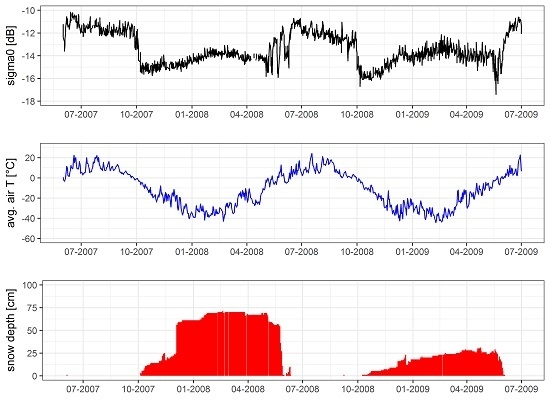
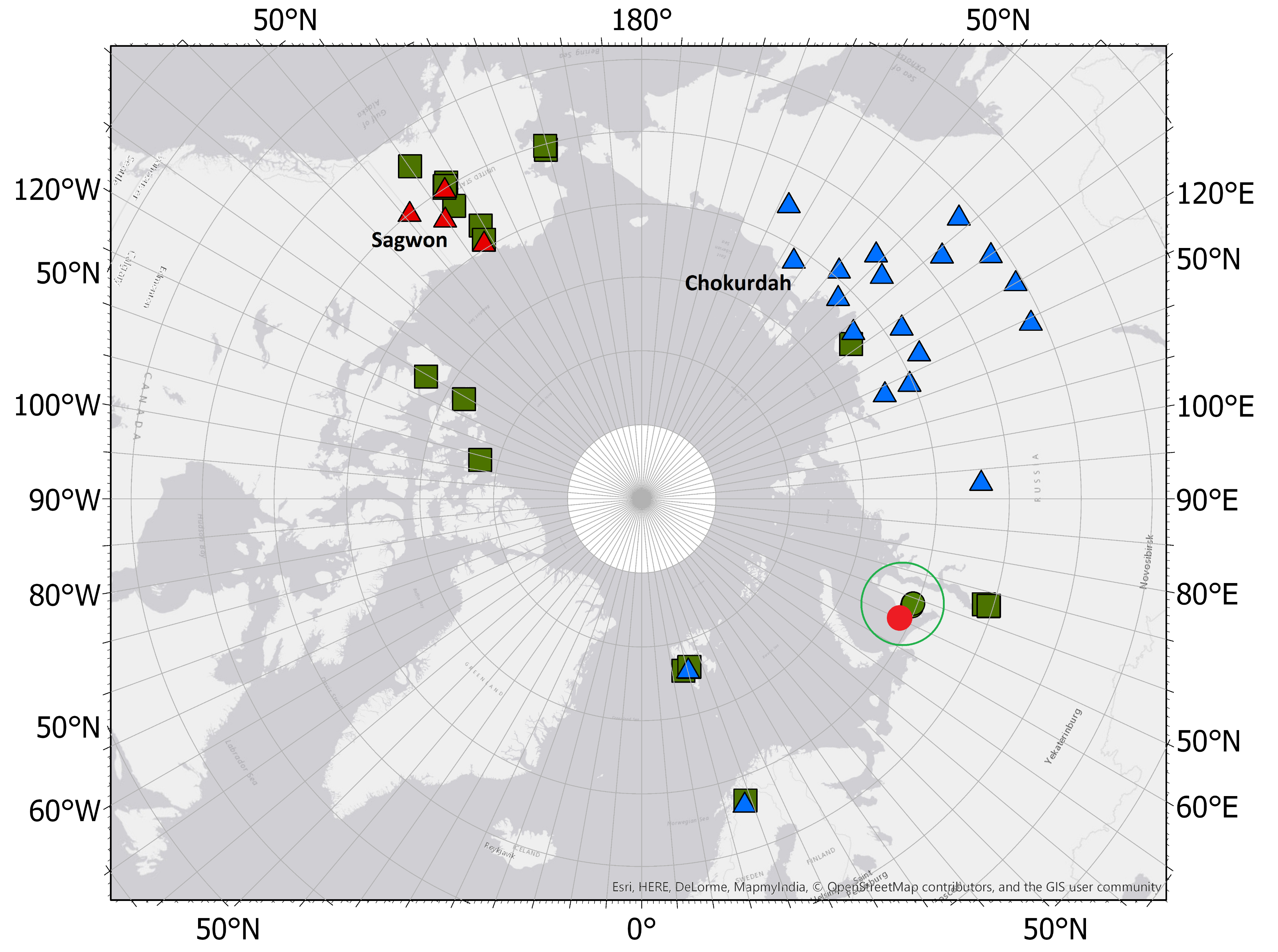
2.1. In Situ Air Temperature and Snow Depth Data

The air temperature and snow depth data sets were obtained for 19 WMO stations in Russia, Alaska (USA), northern Canada and Scandinavia and four SNOTEL stations in Alaska (USA). Covered time periods vary between stations. Air temperature and snow depth data for WMO and SNOTEL stations are given as daily mean values.

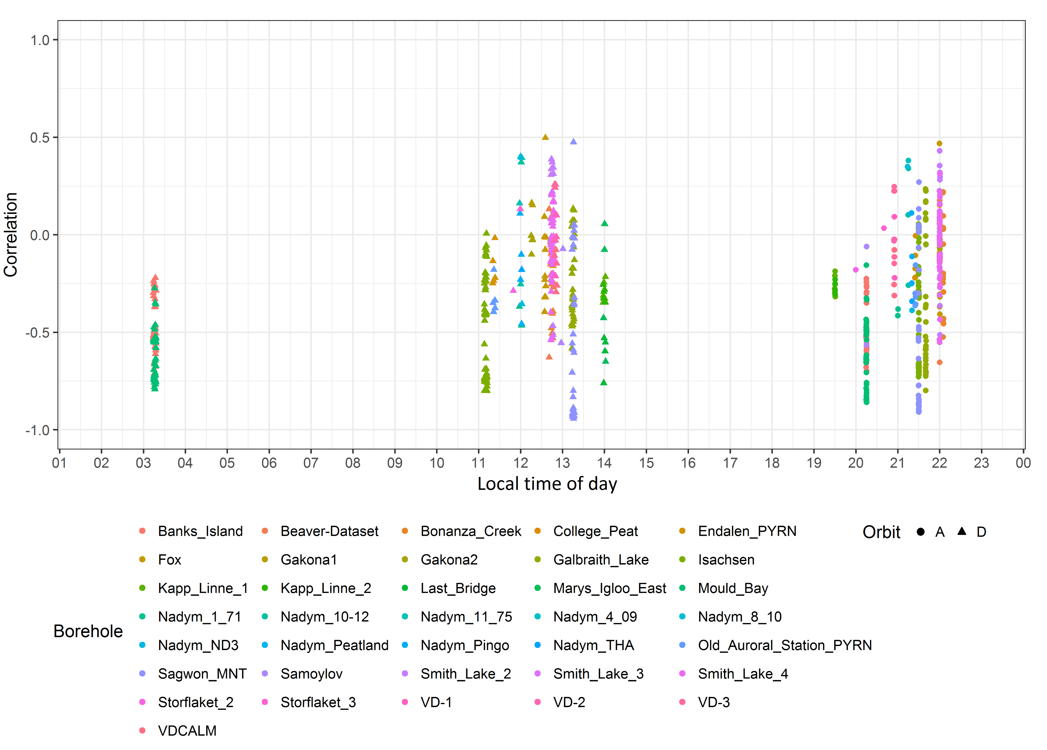
2.2. In Situ Ground Temperature Data

We used in situ ground temperature data obtained from the global terrestrial network for permafrost (GTN–P) [46,47]. The GTN–P database offers data for surface and ground temperature measurements, for a growing number of sites. Measurement sites were chosen according to data availability during the time period of 2007–2016 (ASCAT availability) and the availability of measurements from surface level to a depth of 100 cm. The chosen datasets differ in time series length and measurement frequency.

In addition to the data obtained from the GTN–P database, we used ground temperature time series from four sites at the Vaskiny Dachi research station on Central Yamal, Siberia. Ground temperature measurements at this station were first done in 1993 [48]. Boreholes are equipped with HOBO data loggers [48] and measure ground temperature at different depths (near–surface, 10 cm, 25 cm, 50 cm, and 100 cm). In total, we use ground temperature measurements from 36 boreholes. We subset the data identically to the procedure described above and used the availability of ASCAT backscatter data temporal boundaries.

2.3. ASCAT Backscatter Data

The scatterometer data were obtained from the ASCAT sensor on board the Metop satellites (A and B). The ASCAT is a C–band (5.255 GHz, VV–polarization) instrument [49]. The available records (backscatter, sigma0 (${\sigma }^0$)) have a resolution of 25 km and correspond to different incidence angles. The measurements were re–gridded to a 12.5 km grid [49] and the incidence angles are normalized to a one value at 40° by a procedure described in [50]. Records have been obtained from the EUMETSAT repository (data product ASCAT Soil Moisture at 12.5 km Swath Grid–Metop) and time series for each site covering the years 2007 to 2017 and was individually subset depending on the temporal availability of in situ data at the different sites. The ASCAT data used throughout this study were given in decibel (dB) and is reprocessed according to the WAter Retrieval Package 5 (WARP5) algorithm accounting for noise including instrument noise, speckle and azimuthal anisotropies [50,51].

2.4. Additional Datasets

For the further interpretation of the results, we used additional datasets. To analyze the association with permafrost type we used long–term freezing and thawing indices. Frauenfeld et al. [52] describe a long–term freezing and thawing index for the northern hemisphere which is accessible at [53]. This dataset is based on long–term temperature datasets from 1901–2002 and shows no gaps in the areas considered in this study. The freezing and thawing index is understood to be related to the mean annual air temperature and with that to the permafrost type [52]. Therefore, we used the difference in freezing indices to group the data and discover possible relationships between permafrost type and backscatter dependencies.

To ananylse our results with respect to landcover, we used the GLC2000 landcover map of Northern Eurasia [54] and North America [55] from the Global Land Cover 2000 Project (GLC2000) [56] and the vegetation map of the Norsk Polarinstitutt [57], as the measurement stations on Svalbard are not covered by the GLC2000. To make the the landcover types more comparable between the maps, we summarized them to low vegetation (includes the landscape types Tundra, Consolidated Rock/Sparse Vegetation, Polar Grassland and Subpolar Grassland), medium vegetation (includes the landscape types Sedge Tundra, Prostrate Shrub Tundra, Shrub Tundra and Shrubs), forest (includes the landscape types Subpolar Needleleaved Evergreen Forest, Temperate or Sub–polar Needleleaved Evergreen Forest and Deciduous Needle–leaf Forest), lake rich (includes the landscape type Water bodies), and bogs (includes the landscape type Bogs and marches). To include the soil type in our analysis we extracted the soil type for all points from the Harmonized world soil database [58].

3. Methods

3.1. Data Selection and Preparation

We confined our analysis to the winter period to exclude situations of wet snow and thawed ground. Wet snow is known to have different backscatter characteristics compared to dry snow [59,60], situations of melting snow were therefore excluded. For this purpose, we only included data from December to March for each year. To take additional precautions in avoiding thawing and freezing conditions a temperature limit of $-5$ °C (daily mean value) was introduced for air temperature as well as ground temperature to exclude situations of melting snow occurring during the selected time period. To take influences of topography into consideration, backscatter values from ascending and descending orbits were treated separately. Additionally to the influence of topography, the acquisition time of the ASCAT backscatter data varies for ascending and descending orbits. To ensure maximum consistency between the different datasets, daily means of temperature measurements were used, as most time series were already given in this format. As we limited our analysis to winter periods, we assume backscatter values from mid–day acquisitions to be less representative of the daily mean. Figure 3 shows average acquisition times for both orbits for the locations of all considered boreholes. For stations where average acquisition times (as seen in Figure 3) during mid–day occurred, we excluded those results from further analysis and used only the evening or night–time measurements. For stations where neither orbits had average acquisition times during mid–day (Banks_Island and Mould_Bay), mean values of the correlations of both orbits where used in the final analysis.

We considered available temperature measurements for depths up to 1 m. Measurements were grouped into 0.1 m classes from 0.1 m to 1 m, and 5 cm classes for near surface measurements (see Figure 4 and Figure 5). Studying depths up to 1m allowed us to account for differing penetration depths of ASCAT backscatter (differing between sites as well as during the frozen season) and a possibly decreasing association between ASCAT backscatter and ground temperatures with depth. Additionally, for sites lacking sensors for near–surface measurements, this allowed us to study the association of backscatter and ground temperature despite a lack of near–surface temperature measurements. This is possible as temperature measurements from different depths are assumed to be highly correlated and reasonable assumptions can be made well below the effective sampling depth [61]. The penetration depths of the microwave signal has been shown to decrease with increasing moisture content [15] and C–band microwaves are known to penetrate approximately the upper 5 cm of the soil (e.g., [13,62]). For frozen soil, the penetration depth of the microwaves has been shown to be significantly higher compared to wet soil [28,29,63,64,65,66]. For C–band the penetration depth for frozen soil has been shown to be up to 9 cm deeper compared to thawed conditions [63,64]. For the detailed analysis of the results (including comparisons between different landscape types and soil textures) we focus on the upper 20 cm. This still allows for variable penetrations depths [67,68] (especially considering deeper penetration for frozen conditions) but avoids misconceptions of interactions of backscatter and ground temperature from deeper measurements.

The data were tested for normality of the noise term to judge the reliability of the resulting p–values. The normality of the residuals was tested employing the Anderson–Darling test [69]. To minimize the influence of autocorrelation (which is presumed to be strong if two measurements occur in quick succession), we only considered measurements at most every second day.

To make sure the length of the time series was appropriate for statistical analysis, we excluded sites where only one year was available as well as those where less than 100 winter values remained after the previously described steps.

3.2. Correlation of In Situ Variables with ASCAT Backscatter

To quantify the association between the time series of air temperature, snow depth and ground temperature with ASCAT, backscatter we used the Pearson Correlation coefficient. We calculated correlations for each location seen in Figure 2. To investigate inter annual variations, all calculations were done once separately for each year and once combining all the available years.

To investigate a possible relationship of freezing index and backscatter dependency on ground temperature we created two groups depending on the dataset [53] presented in [52]. A freezing index of 4000 degree–days was chosen as the threshold dividing the data into a warm and a cold group for comparison. The value was chosen in agreement with Smith and Riseborough [70] who have reported that this value corresponds to a MAAT of approx. $-8$ °C and southern limits of continuous permafrost. Gruber [71] have found this to correspond to about 90% of permafrost extent. A possible relationship of the results with the present landcover was investigated using aggregated landcover classes (low vegetation, medium vegetation, Forest, lake rich) based on the GLC2000 landcover map of Northern Eurasia [54] and North America [55] and the vegetation map of the Norsk Polarinstitutt [57]. Results were also analyzed for possible differences between soil textures [58].

3.3. ANCOVA Analysis of ASCAT Backscatter and In Situ Variables

To analyze the dependence of C–band backscatter values on snow depth, air and ground temperature, we apply a common statistical technique: the Analysis of Covariance (ANCOVA). As snow depth and ground temperature values were generally not available for the same stations, we separated them in this analysis, creating one model for snow depth and air temperature and one model for ground temperatures of different depths individually. The dependence of backscatter on the variables ground and air temperature as well as snow depth is assumed to be linear in nature. To account for differences between years, we introduce the year as a categorical variable into the model. The aim of this analysis is to get a sound understanding of how ASCAT backscatter values (in dB) vary with respect to air temperature, snow depth and ground temperature. The models were set up as

$${\sigma }_{i,j}^0=a_i+b_i{T}_{i,j}+c_i{S}_{i,j}+{ϵ}_{i,j}$$

(1)

with backscatter (${\sigma }^0$), air temperature in °C (T), snow depth in cm (S) and the noise term ($ϵ$) and

$${\sigma }_{i,j}^0=a_i+d_{i}G{T}_{i,j}+{ϵ}_{i,j}$$

(2)

with ground temperatures in °C ($GT$). Subscripts encode the year (i) and the number of the observation (j) in the respective year. To quantify the importance of including the year as a categorical variable in the model, we set up a second set of models without accounting for possible differences between the years. These models were set up a

$${\sigma }^0=a+bT+cS+ϵ$$

(3)

with backscatter (${\sigma }^0$), air temperature in °C (T), snow depth in cm (S) and the noise term ($ϵ$) and

$${\sigma }^0=a+dGT+ϵ$$

(4)

with ground temperatures in °C ($GT$). The models were compared using the Analysis of Variance (ANOVA) method (Equations (1)–(4), respectively). The improvement of the models by including the year as a categorical variable was judged by the reduction of the residual sum of squares (RSS) when including the year and whether this reduction was significant ($p<0.05$). For further analysis of the results (b, c, d) dependency on the long–term freezing index (as an indicator of permafrost type), landscape type and soil texture, groups were chosen as described in the previous section.

4. Results

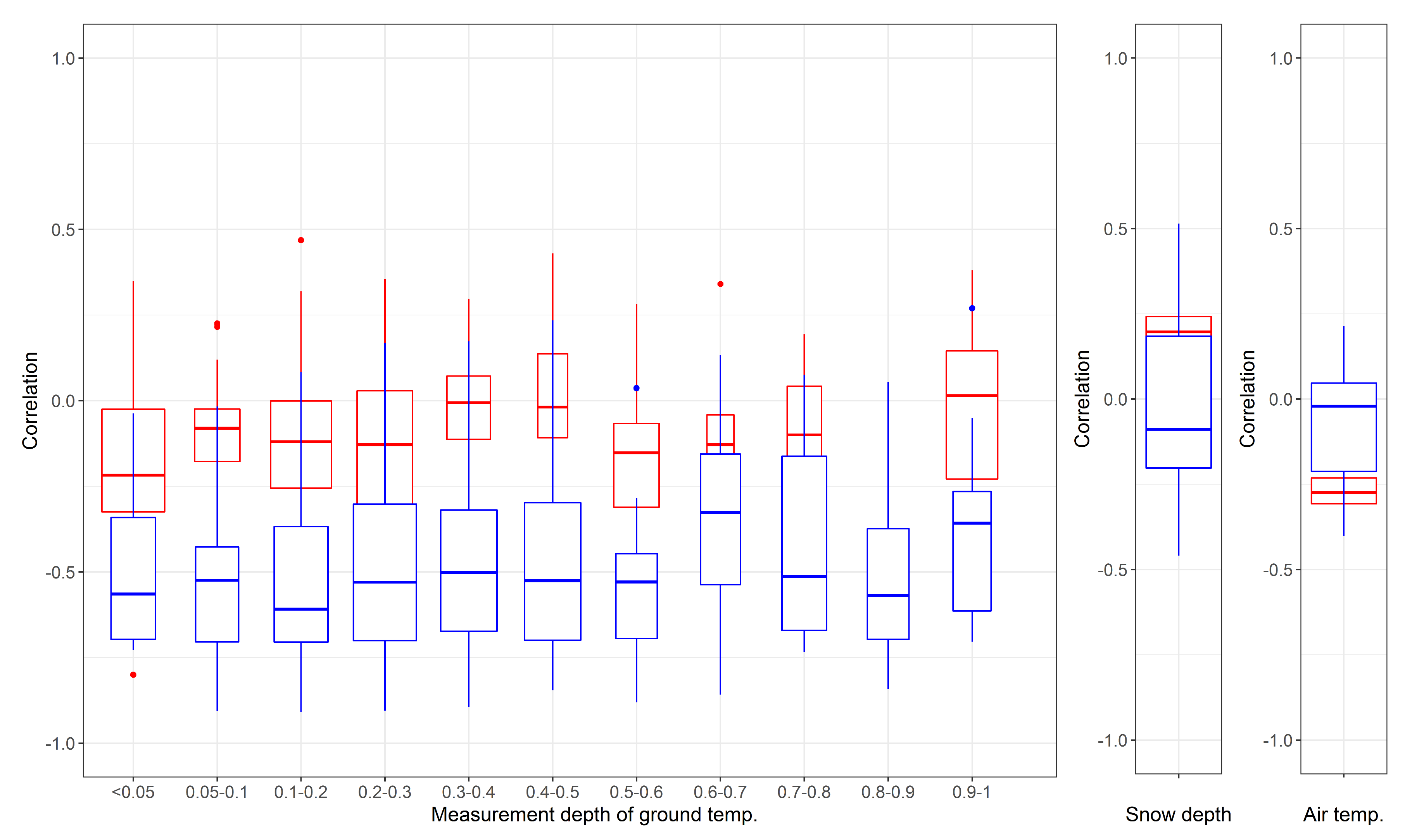
4.1. Correlations of ASCAT Backscatter with Air Temperature, Snow Depth and Ground Temperature

Figure 4 shows strong correlations of backscatter with ground temperature (grouped for different depths) for depth up to 0.6 m for sites with with a freezing index higher than 4000 degree–days. The variables snow depth and air temperature show median correlations closer to 0. Median correlations of backscatter and ground temperature are consistently at or below $-0.5$ for all depths smaller than 0.6 m for sites with high freezing indices (above 4000 degree–days). Correlations for backscatter with ground temperature have overall stronger values (see Figure 4) compared to correlations of backscatter with air temperature and snow depth measurements. Correlations for all three parameters were found to be positive and negative, however strong correlations (<−0.5, >0.5) are negative for ground temperature in all depth groups. Additionally, Figure 4 highlights the differences in data availability in the different depth groups for areas above and below a freezing index of 4000 degree–days through the width of the boxplots. The largest difference between the two groups was found for the depth between 5 and 20 cm (Figure 4). Correlations of backscatter and near–surface (<5 cm) temperature measurements revealed no significant difference between the two groups (see Figure 4), however only the group with the higher freezing indices showed correlation coefficients significantly different from 0. The results reveal no apparent differences between median correlations of backscatter and ground temperature of different depths.

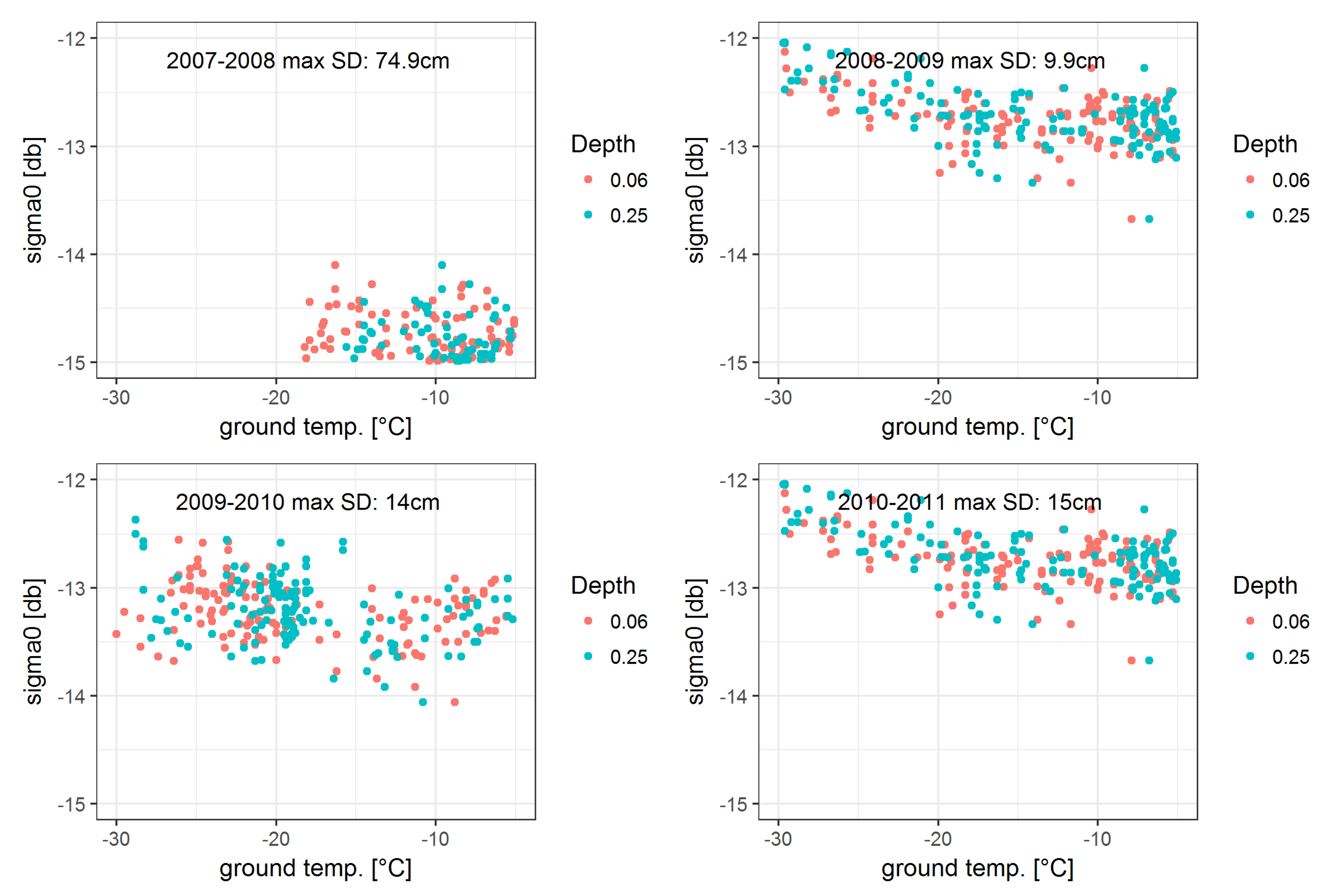
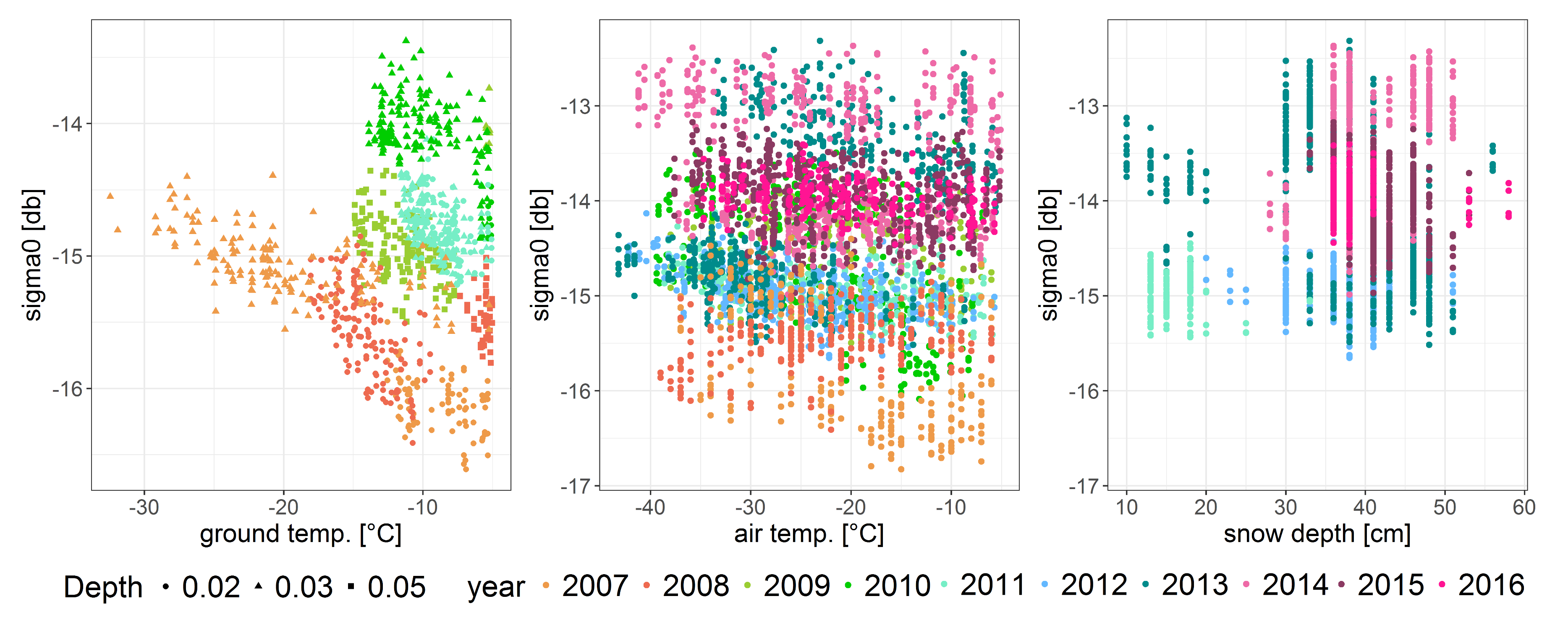
4.2. Analysis of Covariance for ASCAT Backscatter, Air Temperature, Snow Depth and Ground Temperature

Table 1. SNOTEL (S) and WMO stations, Orbits (O) for ASCAT measurements (A, Ascending; D, Descending; and B, average from both), Landcover (LC), Permafrst type (PT), long–term average freezing index in degree–days (FI), results for pearson correlation for snow depth (C. snow) and air temperature (C. air), estimated parameters for snow depth (c) and air temperature (b) with significance (*** $\widehat{=}p<0.01$, ** $\widehat{=}p<0.05$) level.

Station	Lat	Lon	O	LC	PT	FI	C. Snow	c (dB/cm)	C. Air	b (dB/°C)
Sagwon (S)	69.42	−148.69	A	low veg.	cont	4246	0.247	0.02 ***	0.005	0.009 ***
Fairbanks (S)	64.85	−147.8	A	low veg.	dis	2886	0.286	0.018 ***	−0.188	−0.016 ***
Fort Yukon (S)	66.57	−145.25	A	Forest	dis	3360	0.197	0.019 ***	−0.339	−0.028 ***
American Creek (S)	64.79	−141.23	A	Forest	dis	3476	−0.026	−0.001	−0.275	−0.016 ***
Abisko	68.36	18.82	A	Bogs	dis	2025	0.442	0.005 ***	−0.26	−0.013 ***
Agata	66.91	93.38	A	Lake rich	cont	4885	0.2	0.014 ***	0.213	0.015 ***
Dzalinda 1	70.13	113.97	A	Forest	cont	5897	−0.036	0.018 ***	−0.402	−0.028 ***
Saskylah	71.97	114.08	A	med. veg.	cont	6279	−0.376	−0.004	0.088	0.01
Lensk	60.75	114.84	A	Forest	spor	4258	−0.214	−0.011 **	−0.33	−0.002
Suhana	68.62	118.33	A	Forest	cont	5793	−0.079	0.006 **	0.163	0.0003
Oleminsk	60.41	120.45	A	Forest	iso	4235	0.039	−0.002	−0.035	−0.018 ***
Igarka	68.73	124	A	Lake rich	cont	6005	−0.403	−0.003	0.016	−0.014 ***
Isit	60.8	125.37	A	med. veg.	iso	4729	0.138	0.01 ***	−0.008	0.007
Tiksi	71.58	128.92	A	med. veg.	cont	7072	−0.099	−0.003	0.075	−0.001
Batamaj	63.517	129.483	A	Forest	cont	5671	0.514	0.031 ***	−0.349	−0.026 ***
Abramovskij Majak	60.9	131.983	A	Forest	cont	5422	0.235	0.008 ***	0.009	0.012 ***
Bajkit	67.567	133.4	A	Forest	cont	6952	0.229	0.03 ***	−0.383	−0.026 ***
Jubilejnaja	70.77	136.22	A	Lake rich	cont	7197	−0.109	−0.009 ***	−0.208	−0.035 ***
Ust Charky	66.8	136.68	A	Forest	cont	7391	−0.1	−0.004	0.057	−0.009 ***
Deputatskij	69.33	139.67	A	Forest	cont	7478	−0.168	0.002	−0.213	0.021 ***
Chokurdah	70.617	147.883	A	med. veg.	cont	5954	−0.304	−0.008	0.208	−0.0001
Sredhekolymsk	67.45	153.72	A	Lake rich	cont	5609	−0.459	0.019 ***	−0.131	0.007
Svalbard Airport	78.25	15.4667	A	low veg.	cont	3428	0.132	0.005 ***	−0.184	−0.005 **

and

Table 2. Overview of GTN–P boreholes and the Orbits (O) for ASCAT measurements (A, Ascending; D, Descending; and B, average from both), Landcover (LC), Permafrst type (PT), Soil type (ST), long–term average freezing index in degree–days (FI), average pearson correlation for the upper 20 cm (Corr) and estimated parameters (d) for ground temperature with significance (*** $\widehat{=}p<0.01$, ** $\widehat{=}p<0.05$) level; Boreholes with no values for correlation and d lack sufficient measurements in the upper 20 cm.

Borehole	Lat	Lon	O	LC	PT	ST	FI	Corr	d (dB/°C)
Banks_Island	73.22	−119.56	B	low veg.	cont	Regosol	5729	−0.521	−0.004 **
Beaver-Dataset	66.36	−147.39	A	low veg.	dis	Gleysol	3311	−0.655	−0.073 ***
Bonanza_Creek	64.71	−148.29	A	med. veg.	dis	Gleysol	2774	0.002	−0.014
College_Peat	64.87	−147.75	A	med. veg.	dis	Gleysol	2863	−0.103	−0.017
Endalen_PYRN	78.19	15.78	A	low veg.	cont	-	3428	−0.218	−0.063 ***
Fox	64.95	−147.62	A	med. veg.	dis	Gleysol	3083	−0.138	−0.034
Gakona1	62.39	−145.15	A	Forest	cont	Gleysol	2702	0.070	0.014
Gakona2	62.39	−145.15	A	Forest	cont	Gleysol	2702	−0.054	−0.034
Galbraith_Lake	68.48	−149.50	A	low veg.	cont	Leptosol	4467	-0.503	−0.028 **
Isachsen	78.78	−103.55	A	low veg.	cont	Regosol	6963	−0.396	−0.013
Kapp_Linne_1	78.06	13.64	A	low veg.	cont	-	2908	−0.187	−0.065 ***
Kapp_Linne_2	78.05	13.64	A	low veg.	cont	-	2908	−0.252	−0.076 ***
Last_Bridge	65.39	−164.66	A	low veg.	cont	Gleysol	2553	−0.627	−0.129 ***
Marys_Igloo_East	65.11	−164.70	A	low veg.	dis	Gleysol	2527	−0.337	−0.031
Mould_Bay	76.23	−119.30	B	low veg.	cont	Regosol	6550	−0.613	−0.028 ***
Nadym_1_71	65.31	72.82	A	Forest	dis	Fluvisol	3101	−0.398	−0.081 ***
Nadym_10-12	65.30	72.88	A	Bogs	dis	Fluvisol	3101	0.041	−0.038 ***
Nadym_11_75	65.30	72.86	A	Bogs	dis	Fluvisol	3101	0.102	0.031
Nadym_4_09	65.32	72.88	A	med. veg.	dis	Fluvisol	3101	-	-
Nadym_8_10	65.67	72.87	A	Lake rich	dis	Histosol	3107	-	-
Nadym_ND3	65.31	72.86	A	med. veg.	dis	Fluvisol	3101	−0.388	−0.022 ***
Nadym_Peatland	65.30	72.89	A	Bogs	dis	Fluvisol	3101	-	-
Nadym_Pingo	65.30	72.90	A	med. veg.	dis	Histosol	3101	−0.082	−0.01
Nadym_THA	65.32	72.86	A	med. veg.	dis	Fluvisol	3101	-	-
Old_Auroral_Station_PYRN	78.20	15.83	A	low veg.	cont	-	3428	−0.298	−0.05 ***
Sagwon_MNT	69.43	−148.67	A	low veg.	cont	Gleysol	4248	−0.487	−0.09 **
Samoylov	72.37	126.48	A	low veg.	cont	Fluvisol	6967	−0.313	−0.049 ***
Smith_Lake_2	64.87	−147.86	A	Forest	dis	Gleysol	2863	0.106	−0.02
Smith_Lake_3	64.87	−147.86	A	Forest	dis	Gleysol	2863	−0.259	−0.237 ***
Smith_Lake_4	64.87	−147.86	A	Forest	dis	Gleysol	2863	−0.063	0.015
Storflaket_2	68.35	18.97	A	Bogs	dis	-	2025	-	-
Storflaket_3	68.35	18.97	A	Bogs	dis	-	2025	0.033	0.005
VD-1	70.28	68.89	A	med. veg.	cont	Gleysol	3567	0.092	0.189
VD-2	70.30	68.88	A	med. veg.	cont	Gleysol	3567	-	-
VD-3	70.30	68.84	A	med. veg.	cont	Gleysol	3567	-	-
VDCALM	70.28	68.91	A	med. veg.	cont	Gleysol	3567	−0.077	0.185

summarize the results of the ANCOVA analysis for the three tested parameters air temperature, snow depth and ground temperature (based on Equations (1) and (2)). For the analysis of snow depth and air temperature, 14 out of 22 for snow depth and 15 out of 22 for air temperature showed significant results ($p<0.05$). However, the stations with significant results for snow depth and air temperature were not entirely the same ones. The analysis of ground temperature showed that the percentage of significant results for the estimated parameter is highest in the upper 10 cm, with 88% of parameters for these measurements being significant for sites with freezing degree days above 4000 degree days (see

Table 3. Percentage of significant negative parameter coefficients (p < 0.05) resulting from the ANCOVA analysis for ground temperatures (depths of 0–1 m) divided into sites with freezing degree days above and below 4000 degree–days.

Depth in m	<0.1	0.1–0.2	0.2–0.3	0.3–0.4	0.4–0.5	0.5–0.6	0.6–0.7	0.7–0.8	0.8–0.9	0.9–1
>4000 degree–days	88%	68%	84%	60%	52%	32%	28%	48%	16%	28%
<4000 degree–days	71%	26%	24%	11%	15%	8%	4%	8%	0%	22%

). The percentage of significant results for warmer sites (below 4000 degree–days) is lower compared to colder sites for all measurement depths. A comparison of the estimated parameters of air temperature, snow depth and ground temperature revealed, that while both air temperature and snow depth show both positive as well as negative significant parameters, all significant parameters for ground temperatures (in the upper 20 cm) are negative (see Table 1 and Table 2).

Figure 5 shows the results of the ANCOVA analysis in form of the estimated parameters for backscatter dependencies on ground temperature (grouped for different depths), snow depth and air temperature using separate axis for the three parameters due to the different units. The results show no significant differences between the two groups of sites with freezing indices above or below 4000 degree–days for all of the three variables. Additionally, there are no significant differences for the results for ground temperature in different depths. Except for outliers, the results for all depth groups as well as for both the group with higher (≥4000 degree–days) and lower (<4000 degree–days) freezing indices have values close to zero. The estimated parameter for ground temperature (d) varies mainly between 0.15 dB/°C and −0.15 dB/°C. Snow depth (c in dB/cm) and air temperature (b in dB/°C) show similar numbers, however these parameters are not directly comparable as they have different units. The estimated parameter for ground temperature however shows larger variations (for most depth groups) compared to the other variables (see Figure 5).

Figure 6 shows backscatter values and ground temperature values for a borehole on central Yamal (VD–1) for selected years, highlighting the differences between different years and the importance to include values from more than one winter. The difference between the parameters is visualized in Figure 7 which shows values for all parameters for all available years. Furthermore, the comparison of the different models including and excluding the year as a categorical parameter (Equations (1)–(4)) showed an improvement when the difference between the years is accounted for. The comparison revealed a significant improvement for 96% of the sites for air temperature and snow depth and for 65% of the borehole locations.

The results of the analysis of normality of the residuals is shown in

Table 4. Results of the normality test of the residuals for the ANCOVA analysis (air temperature, snow depth, ground temperature (for the different depth groups in m)). $N_{norm}$ gives the relative number of occurrences (normalized by the total number of sites relevant for this parameter), for which the deviation from normality is significant at $\alpha =0.01$.

Variable	${\mathit{N}}_{\mathbf{norm}}$ (%)
Air temp. and snow depth	75.67
Ground temp. <0.05	72.72
Ground temp. 0.05–0.1	50
Ground temp. 0.1–0.2	61.66
Ground temp. 0.2–0.3	56.75
Ground temp. 0.3–0.4	40.74
Ground temp. 0.4–0.5	61.36
Ground temp. 0.5–0.6	50
Ground temp. 0.6–0.7	40.90
Ground temp. 0.7–0.8	44.11
Ground temp. 0.8–0.9	28.57
Ground temp. 0.9–1	60

. Results show approximately half of the tested residuals can be assumed to be normally distributed with a significant level of 0.01.

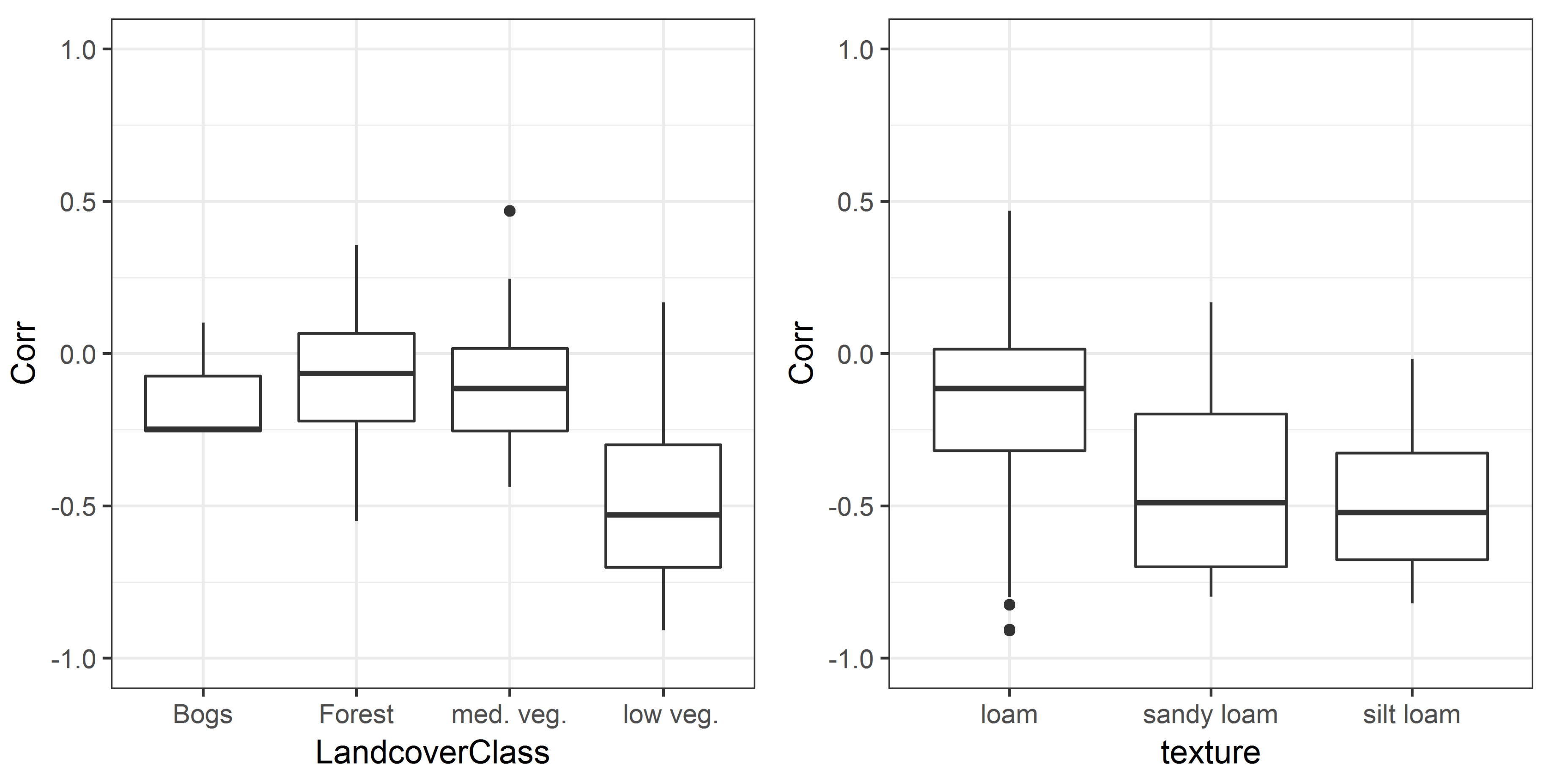
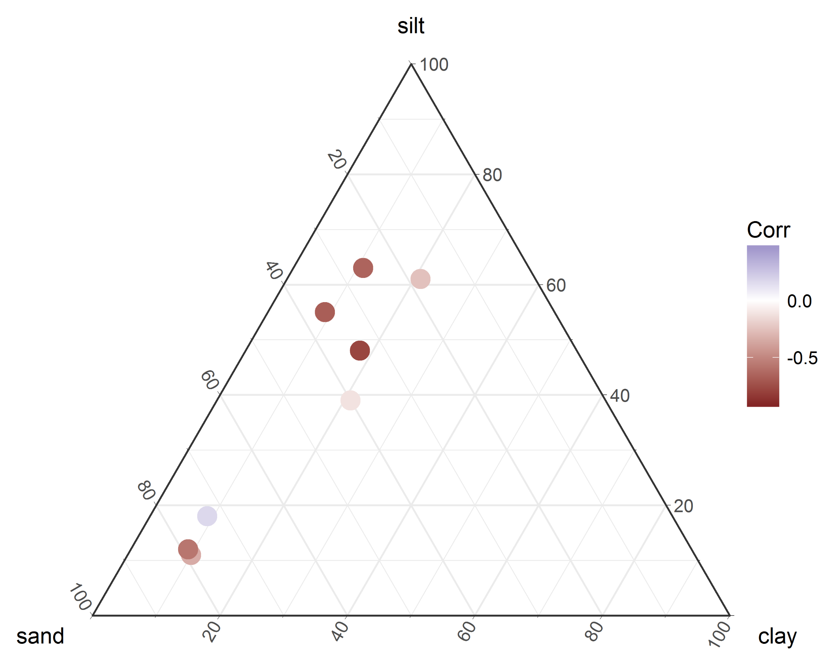
4.3. Influence of Landscape and Soil Type on Ground Temperature Dependency

The influence of landscape and soil type on ground temperature is shown in Figure 8. The comparison (as shown in Figure 8) shows that points with low vegetation have higher (negative) correlations between ASCAT backscatter and ground temperature compared to other landcover classes. Points with soil textures sandy loam and silt loam have the lowest median correlations, compared to all present classes. The estimated parameter for ground temperature shows fewer differences between the groups (for landcover and soil texture), however the landcover class medium vegetation and the soil texture class loam show a high number of outliers.

5. Discussion

This study examined correlations and dependencies of ASCAT C–band backscatter on air and ground temperature as well as snow depth. Results indicate a relationship of the backscatter to subsurface properties raising the question of penetration depth. Depending on soil type, frozen or thawed conditions and vegetation cover, the penetration depth of C–band backscatter varies [64,73]. During the freezing process, penetration depth is likely to increase, causing an increase in volume scattering through interaction of the radar signal with soil particles. We suspect this to be contributing to the increase in backscatter with dropping temperatures exemplified in Figure 1, Figure 6 and Figure 7 and causing the strong negative correlations mainly exhibited by measurements in the upper 20 cm in areas with high freezing indices (above 4000 degree–days). In addition, the change of dielectric constant with with temperature under frozen conditions needs to be considered. In the field of scatterometer based ice–sheet and scatterometer applications, the relationship of ASCAT backscatter and snow characteristics has been examined in multiple studies (e.g., [41,74]). Fraser et al. [41] found negative correlations of ASCAT backscatter and surface temperature of snow and link this to a change of dielectric constant with temperature. Bingham and Drinkwater [75] reported similar findings for analysis using European Remote–Sensing Satellite (ERS) C–band scatterometer and Special Sensor Microwave/Imager (SSM/I) image data. The negative correlations found by [41] are based on surface temperature (of snow) considering a time lag for propagation of surface temperature cycles/anomalies downward through the firn. Our analysis also found significant results for measurements in the soil down to a depth of 20 cm.

In contrast to the predominantly colder sites, sites with a mean freezing index below 4000 did not show pearson correlation coefficients significantly different from 0 regardless of depth. This could be interpreted as the absence of the underlying phenomenon in warmer areas. Liquid water may still be present [31]. Another possibility is that in situ measurements may not be representative. Warmer areas are more heterogeneous (possibly discontinuous or sporadic permafrost). Ground temperature measurements, which are point measurements, might not be representative in such environments (often chosen at special sites that have permafrost) and therefore lack correlation with backscatter values which represent a large area, a problem which is at least partially excluded in the areas with continuous permafrost. Additionally, areas with lower freezing indices can be expected to have higher temperatures during the course of the winter which in turn can cause increased snow metamorphism processes like depth hoar [76].

Due to issues of data scarcity, the analysis of air temperature and snow depth was mostly done using data from different stations compared to the sites used for the analysis of ground temperature, and for sites where data for all variables was available the measurement times did not necessarily overlap. We assume that the interactions between snow and backscatter are not site specific. This is underlined by the small variance found for the parameter c. It would however be of great interest to study this phenomenon in more detail using a study site which is highly instrumented, not only measuring air temperature, snow depth and soil temperature but also soil moisture. To the best of our knowledge, the sites in existence (such as Barrow in Alaska, Samoylov and Tiksi in the Lena Delta region) lack representativeness for the ASCAT footprints (close to coastlines, special cases). Analyses with higher resolution Synthetic Aperture Radar data would be required. Missions such as Sentinel–1 may provide the necessary temporal sampling. To study this phenomenon in detail across the Arctic with different landscape and soil types as well as different latitudes, a multitude of these super–sites would be of great importance.

The differences in correlation of backscatter and ground temperature in Figure 8 have to be seen in context with

Table 5. Percentage of boreholes (with ground temperature sensors in the upper 20 cm) of different soil textures (loam, sandy loam and silt loam) for different landscape types (low vegetation, medium vegetation, forest, and bogs).

Soil Textures	Low Vegetation	Medium Vegetation	Forest	Bogs
Loam	20.2%	86.6%	97.7%	0%
Sandy loam	16.25%	6.6%	2.8%	100%
Silt loam	63.5%	6.6%	0%	0%

and Figure 9. The two soil texture classes with the strongest correlations (sandy loam and silt loam) both mainly occur (in this study) for sites with low vegetation (see Table 5) which is also the landscape class with the strongest negative correlations in the upper 20 cm (see Figure 8). The soil texture class loam, which shows the highest variability for the parameter d (Figure 8), overlaps with the landcover classes low vegetation, medium vegetation and forest. Comparing the boxplots for landcover and soil texture classes, the landcover class medium vegetation shows a similar pattern of outliers. From this analysis it can not be conclusively said, if soil types or landcover class are more influential on the backscatter–ground temperature relationship.

Additionally, landcover classes can not be seen as independent from the mean annual air temperature and with that the permafrost type. Therefore, the strong correlations for boreholes with low vegetation (see Figure 8) and the strong correlations for the boreholes with long–term freezing indices above 4000 degree–days have to be seen as highly overlapping.

Overall, we did not find strong correlations between ASCAT backscatter and snow depth time series in this analysis. At C–band, depth hoar formation, which is itself closely related to temperature [76], could be more important [77]. It could also be hypothesized that while there is no direct relationship of snow depth and backscatter at C–band, that snow, if it reaches a certain depth, strongly influences the ground temperature regime [78]. This is amplified for sites where snow reaches a high level before the onset of the ground freezing [79]. An analysis of both the influence of depth hoar formation on backscatter and the influence of differing snow levels between years on the relationship of backscatter and ground temperature would require a more comprehensive dataset than currently available.

Another issue influencing correlation results are variations of the backscatter level during the relevant periods. Variations in backscatter level (as seen in Figure 6) occur between different years. In the case of Yamal, it can differ in the order of 2 dB. Differing backscatter levels can be caused by depth hoar or rain on snow events and the subsequent formations of ice layers on or within the snow pack [80], which is a known phenomenon in the region of Yamal, Russia where the borehole is located [80,81] as well as in other arctic areas [82,83]. Rain on snow has been shown to occur here specifically in November with subsequent impact on ASCAT backscatter (minimum 0.5 dB increase [81]). The relationship to subsurface temperature does however prevail. The different levels between the years highlight the importance of separating the years when using multi–year datasets. Figure 6 also highlights the connection of backscatter level and maximum snow depth as the winter of 2007–2008 show by far the highest maximum snow depth (74.9 cm) and a 2 dB backscatter difference compared to the other years. The winter of 2007–2008 shows not only lower backscatter values but also overall less variations of backscatter. This can also be seen for WMO station Chokurdah (see Figure 1) which shows higher variations in backscatter during the winter 2008–2009 which has comparatively little snow. These winter–time backscatter variations could introduce strong biases into freeze/thaw and SWE retrieval algorithms, both of which tend to neglect winter–time processes. Higher values during winter have the potential of distorting thresholds used for freeze/thaw classifications. The low correlations of backscatter and snow depth, as well as the low variations shown in the backscatter time series during winter 2007–2008 for Chokurdah (see Figure 1), imply a possible underestimation of the total SWE.

While ANCOVA has been shown to be relatively robust to the violation of the assumption of normality of the residuals [84,85,86], the parameter of dependence of backscatter on air temperature, snow depth and ground temperature has to be seen together with the results reported in Table 4; p–values of the estimated parameters might therefore not be reliable in some cases.

Our findings show that, at C–band, interactions of backscatter with the ground during winter months cannot be ruled out. We found strong correlations of backscatter and ground temperatures during that time. We also see a difference between continuous and discontinuous permafrost sites. This suggests the possibility of separating continuous and non–continuous (discontinuous, sporadic and isolated) areas through the backscatter behaviour over time and with that enhancing the mapping of it’s extent and distribution.

6. Conclusions

This study examines the relationship of ASCAT backscatter with air temperature and snow depth for 21 sites and the relationship of backscatter and ground temperature for a total of 36 boreholes. We found strong correlations of winter backscatter and ground temperatures at depths up to 60 cm for cold areas (above 4000 freezing degree–days, likely continuous permafrost). Interactions of backscatter and the ground surface can therefor not be ruled out during winter–time as it might lead to strong biases. Results for the analysis of snow depth and air temperature showed weaker correlations. We found a distinct difference in the correlation of backscatter with ground temperature for cold and warm sites (1600–4000 freezing degree days, likely non–continuous permafrost) which show smaller correlations for all depths. Results are likely impacted by snow metamorphism, the underlying soil and its characteristics as well as vegetation. However, these factors are not independent variables and their influences could not be separated using the available data.

The results highlight the importance and complexity of winter–time processes of all three variables as well as their specific winter–time relationships with C–band backscatter. We conclude that neglecting these processes can introduce strong biases into freeze/thaw and snow characteristics retrieval algorithms. The differences between continuous and non–continuous permafrost sites suggest the possibility of improving the mapping of these features by including winter–time analysis.

References

1. Jones, L.A.; Kimball, J.S.; McDonald, K.C.; Chan, S.T.K.; Njoku, E.G.; Oechel, W.C. Satellite microwave remote sensing of boreal and arctic soil temperatures from AMSR-E. IEEE Trans. Geosci. Remote Sens. 2007, 45, 2004–2018. [Google Scholar] [CrossRef]
2. McDonald, K.C.; Kimball, J.S.; Njoku, E.; Zhao, M. Variability in springtime thaw in the terrestrial high latitudes: Monitoring a major control on the biospheric assimilation of atmospheric CO2 with spaceborne microwave remote sensing. Earth Interact. 2004, 8. [Google Scholar] [CrossRef]
3. Bartsch, A.; Kidd, R.A.; Wagner, W.; Bartalis, Z. Temporal and spatial variability of the beginning and end of daily spring freeze/thaw cycles derived from scatterometer data. Remote Sens. Environ. 2007, 106, 360–374. [Google Scholar] [CrossRef]
4. Wang, L.; Derksen, C.; Brown, R. Detection of pan-Arctic terrestrial snowmelt from QuikSCAT, 2000–2005. Remote Sens. Environ. 2008, 112, 3794–3805. [Google Scholar] [CrossRef]
5. Bartsch, A.; Wagner, W.; Rupp, K.; Kidd, R. Application of C and Ku-band scatterometer data for catchment hydrology in northern latitudes. In Proceedings of the IEEE International Geoscience and Remote Sensing Symposium, Barcelona, Spain, 23–28 July 2007; pp. 3702–3705. [Google Scholar]
6. Semmens, K.A.; Ramage, J.; Bartsch, A.; Liston, G.E. Early snowmelt events: Detection, distribution, and significance in a major sub-arctic watershed. Environ. Res. Lett. 2013, 8, 014020. [Google Scholar] [CrossRef]
7. Woodhouse, I.H. Introduction to Microwave Remote Sensing; CRC Press: Boca Raton, FL, USA, 2005. [Google Scholar]
8. Zhao, T.; Zhang, L.; Jiang, L.; Zhao, S.; Chai, L.; Jin, R. A new soil freeze/thaw discriminant algorithm using AMSR–E passive microwave imagery. Hydrological 2011, 25, 1704–1716. [Google Scholar] [CrossRef]
9. Zwieback, S.; Paulik, C.; Wagner, W. Frozen Soil Detection Based on Advanced Scatterometer Observations and Air Temperature Data as Part of Soil Moisture Retrieval. Remote Sens. 2015, 7, 3206–3231. [Google Scholar] [CrossRef]
10. Derksen, C.; Walker, A.E.; Goodison, B.E. Evaluation of passive microwave snow water equivalent retrievals across the boreal forest/tundra transition of western Canada. Remote Sens. Environ. 2005, 96, 315–327. [Google Scholar] [CrossRef]
11. Pulliainen, J. Mapping of snow water equivalent and snow depth in boreal and sub-arctic zones by assimilating space-borne microwave radiometer data and ground-based observations. Remote Sens. Environ. 2006, 101, 257–269. [Google Scholar] [CrossRef]
12. Högström, E.; Trofaier, A.M.; Gouttevin, I.; Bartsch, A. Assessing Seasonal Backscatter Variations with Respect to Uncertainties in Soil Moisture Retrieval in Siberian Tundra Regions. Remote Sens. 2014, 6, 8718–8738. [Google Scholar] [CrossRef]
13. Naeimi, V.; Paulik, C.; Bartsch, A. ASCAT Surface State Flag (SSF): Extracting information on surface freeze/thaw conditions from backscatter data using an empirical threshold-analysis algorithm. IEEE Trans. Geosci. Remote Sens. 2012, 50, 2566–2582. [Google Scholar] [CrossRef]
14. Park, S.E. Variations of Microwave Scattering Properties by Seasonal Freeze/Thaw Transition in the Permafrost Active Layer Observed by ALOS PALSAR Polarimetric Data. Remote Sens. 2015, 7, 17135–17148. [Google Scholar] [CrossRef]
15. Ulaby, F.T.; Dubois, P.C.; Jakob, V.Z. Radar mapping of surface soil moisture. J. Hydrol. 1996, 184, 57–84. [Google Scholar] [CrossRef]
16. Zhang, L.; Shi, J.; Zhang, Z.; Zhao, K. The estimation of dielectric constant of frozen soil-water mixture at microwave bands. In Proceedings of the 2003 IEEE International Geoscience and Remote Sensing Symposium, Toulouse, France, 21–25 July 2003; Volume 4, pp. 2903–2905. [Google Scholar]
17. Kimball, J.S.; McDonald, K.C.; Frolking, S.; Running, S.W. Radar remote sensing of the spring thaw transition across a boreal landscape. Remote Sens. Environ. 2004, 89, 163–175. [Google Scholar] [CrossRef]
18. Yi, Y.; Kimball, J.S.; Jones, L.A.; Reichle, R.H.; Nemani, R.; Margolis, H.A. Recent climate and fire disturbance impacts on boreal and arctic ecosystem productivity estimated using a satellite-based terrestrial carbon flux model. J. Geophys. Res. Biogeosci. 2013, 118, 606–622. [Google Scholar] [CrossRef]
19. Wang, G.; Hu, H.; Li, T. The influence of freeze-thaw cycles of active soil layer on surface runoff in a permafrost watershed. J. Hydrol. 2009, 375, 438–449. [Google Scholar] [CrossRef]
20. Qi, J.; Vermeer, P.A.; Cheng, G. A review of the influence of freeze-thaw cycles on soil geotechnical properties. Permafr. Periglac. Process. 2006, 17, 245–252. [Google Scholar] [CrossRef]
21. Bartsch, A. Ten Years of SeaWinds on QuikSCAT for Snow Applications. Remote Sens. 2010, 2, 1142–1156. [Google Scholar] [CrossRef]
22. Kimball, J.; McDonald, K.C.; Keyser, A.; Frolking, S.; Running, S. Application of the NASA Scatterometer (NSCAT) for Determining the Daily Frozen and Nonfrozen Landscape of Alaska. Remote Sens. Environ. 2001, 75, 113–126. [Google Scholar] [CrossRef]
23. Frolking, S.; McDonald, K.C.; Kimball, J.; Way, J.; Zimmermann, R.; Running, S. Using the space-borne NASA scatterometer (NSCAT) to determine the frozen and thawed seasons. Remote Sens. Environ. 1999, 104, 27895–27907. [Google Scholar]
24. Rignot, E.; Way, J.B. Monitoring freeze–Thaw cycles along North–South Alaskan transects using ERS-1 SAR. Remote Sens. Environ. 1994, 49, 131–137. [Google Scholar] [CrossRef]
25. Peplinski, N.R.; Ulaby, F.T.; Dobson, M.C. Dielectric properties of soils in the 0.3–1.3-GHz range. IEEE Trans. Geosci. Remote Sens. 1995, 33, 803–807. [Google Scholar] [CrossRef]
26. Osterkamp, T. Freezing and thawing of soils and permafrost containing unfrozen water or brine. Water Resour. Res. 1987, 23, 2279–2285. [Google Scholar] [CrossRef]
27. Ulaby, F.T.; Long, D.G. Microwave Radar and Radiometric Remote Sensing; University of Michigan Press: Ann Arbor, MI, USA, 2014. [Google Scholar]
28. Dobson, M.C.; Ulaby, F.T.; Hallikainen, M.T.; El-Rayes, M.A. Microwave Dielectric Behavior of Wet Soil-Part II: Dielectric Mixing Models. IEEE Trans. Geosci. Remote Sens. 1985, GE-23, 35–46. [Google Scholar] [CrossRef]
29. Hallikainen, M.T.; Ulaby, F.T.; Dobson, M.C.; El-Rayes, M.A.; Wu, L.K. Microwave Dielectric Behavior of Wet Soil-Part 1: Empirical Models and Experimental Observations. IEEE Trans. Geosci. Remote Sens. 1985, GE-23, 25–34. [Google Scholar] [CrossRef]
30. Gupta, S.C.; Larson, W.E. Estimating soil water retention characteristics from particle size distribution, organic matter percent, and bulk density. Water Resour. Res. 1979, 15, 1633–1635. [Google Scholar] [CrossRef]
31. Romanovsky, V.E.; Osterkamp, T.E. Effects of unfrozen water on heat and mass transport processes in the active layer and permafrost. Permafr. Periglac. Process. 2000, 11, 219–239. [Google Scholar] [CrossRef]
32. Konrad, J.M. Physical processes during freeze-thaw cycles in clayey silts. Cold Reg. Sci. Technol. 1989, 16, 291–303. [Google Scholar] [CrossRef]
33. Tice, A.; Black, P.; Berg, R. Unfrozen water contents of undisturbed and remolded Alaskan silt. Cold Reg. Sci. Technol. 1989, 17, 103–111. [Google Scholar] [CrossRef]
34. Konrad, J.M. Unfrozen Water as a Function of Void Ratio in a Clayey Silt. Cold Reg. Sci. Technol. 1990, 1, 49–55. [Google Scholar] [CrossRef]
35. Colbeck, S.C. An overview of seasonal snow metamorphism. Rev. Geophys. 1982, 20, 45–61. [Google Scholar] [CrossRef]
36. Dirmhirn, I.; Eaton, F.D. Some Characteristics of the Albedo of Snow. J. Appl. Meteorol. 1975, 14, 375–379. [Google Scholar] [CrossRef]
37. Alford, D. Density variations in apline snow. J. Glaciol. 1967, 6, 495–503. [Google Scholar] [CrossRef]
38. Pivot, F.C. C-Band SAR Imagery for Snow-Cover Monitoring at Treeline, Churchill, Manitoba, Canada. Remote Sens. 2012, 4, 2133–2155. [Google Scholar] [CrossRef]
39. West, R.D. Potential applications of 1–5 GHz radar backscatter measurements of seasonal land snow cover. Radio Sci. 2000, 35, 967–981. [Google Scholar] [CrossRef]
40. Eckerstorfer, M.; Malnes, E.; Christiansen, H. Freeze/thaw conditions at periglacial landforms in Kapp Linné, Svalbard, investigated using field observations, in situ, and radar satellite monitoring. Geomorphology 2017, 293, 433–447. [Google Scholar] [CrossRef]
41. Fraser, A.D.; Nigro, M.A.; Ligtenberg, S.R.M.; Legresy, B.; Inoue, M.; Cassano, J.J.; Kuipers Munneke, P.; Lenaerts, J.T.M.; Young, N.W.; Treverrow, A. Drivers of ASCAT C band backscatter variability in the dry snow zone of Antarctica. J. Glaciol. 2016, 62, 170–184. [Google Scholar] [CrossRef]
42. Evans, S. Dielectric Properties of Ice and Snow–A Review. J. Glaciol. 1965, 5, 773–792. [Google Scholar] [CrossRef]
43. Stiles, W.; Ulaby, F.T. Dielectric Properties of Snow; Technical Report; NASA: Greenbelt, MD, USA, 1981. [Google Scholar]
44. Hallikainen, M.; Ulaby, F.; Abdelrazik, M. Dielectric properties of snow in the 3 to 37 GHz range. IEEE Trans. Antennas Propagat. 1986, 34, 1329–1340. [Google Scholar] [CrossRef]
45. Bernier, M.; Fortin, J.P. The potential of times series of C-Band SAR data to monitor dry and shallow snow cover. IEEE Trans. Geosci. Remote Sens. 1998, 36, 226–243. [Google Scholar] [CrossRef]
46. Global Terrestrial Network for Permafrost (GTN-P). Global Terrestrial Network for Permafrost Database: Permafrost Temperature Data (TSP Thermal State of Permafrost). 2016. Available online: http://gtnpdatabase.org/ (accessed on 14 December 2016).
47. Biskaborn, B.K.; Lanckman, J.P.; Lantuit, H.; Elger, K.; Streletskiy, D.A.; Cable, W.L.; Romanovsky, V.E. The new database of the Global Terrestrial Network for Permafrost (GTN-P). Earth Syst. Sci. Data 2015, 7, 245–259. [Google Scholar] [CrossRef] [Green Version]
48. Leibman, M.; Khomutov, A.; Gubarkov, A.; Mullanurov, D.; Dvornikov, Y. The research station “Vaskiny Dachi”, Central Yamal, West Siberia, Russia–A review of 25 years of permafrost studies. Fennia 2015, 193, 3–30. [Google Scholar]
49. Figa-Saldaña, J.; Wilson, J.J.; Attema, E.; Gelsthorpe, R.; Drinkwater, M.R.; Stoffelen, A. The advanced scatterometer (ASCAT) on the meteorological operational (MetOp) platform: A follow on for European wind scatterometers. Can. J. Remote Sens. 2002, 28, 404–412. [Google Scholar] [CrossRef]
50. Naeimi, V.; Scipal, K.; Bartalis, Z.; Hasenauer, S.; Wagner, W. An Improved Soil Moisture Retrieval Algorithm for ERS and METOP Scatterometer Observations. IEEE Trans. Geosci. Remote Sens. 2009, 47, 1999–2013. [Google Scholar] [CrossRef]
51. Bartalis, Z.; Wagner, W.; Naeimi, V.; Hasenauer, S.; Scipal, K.; Bonekamp, H.; Figa, J.; Anderson, C. Initial soil moisture retrievals from the METOP-A Advanced Scatterometer (ASCAT). Geophys. Res. Lett. 2007, 34, L20401. [Google Scholar] [CrossRef]
52. Frauenfeld, O.W.; Zhang, T.; Mccreight, J.L. Northern hemisphere freezing/thawing index variations over the twentieth century. Int. J. Climatol. 2007, 27, 47–63. [Google Scholar] [CrossRef]
53. Zhang, T.; Frauenfeld, O.W.; McCreight, J.L.; Berry, R. Northern Hemisphere EASE-Grid Annual Freezing and Thawing Indices, 1901–2002, Version 1. 2005. Available online: https://nsidc.org/data/ggd649 (accessed on 26 January 2017).
54. Belward, A.S.; Erchov, D.V.; Isaev, A.S.; Bartholom, E.; Gond, V.; Vogt, P.; Achard, F.; Zubkov, A.M.; Mollicone, D.; Savin, I.; et al. The Land Cover Map for Northern Eurasia for the Year 2000. GLC2000 Database, European Commision Joint Research Centre. 2003. Available online: http://www-gem.jrc.it/glc2000 (accessed on 22 August 2017).
55. Latifovic, R.; Zhu, Z.; Cihlar, J.; Beaubien, J.; Fraser, R. The Land Cover Map for North America in the Year 2000. GLC2000 Database, European Commision Joint Research Centre. 2003. Available online: http://www-gem.jrc.it/glc2000 (accessed on 22 August 2017).
56. Bartholomé, E.; Belward, A. GLC2000: A new approach to global land cover mapping from Earth observation data. Int. J. Remote Sens. 2005, 26, 1959–1977. [Google Scholar] [CrossRef]
57. Norsk Polarinstitutt. Svalbardkartet. Available online: http://svalbardkartet.npolar.no/html5/index.html?viewer=svalbardkartet (accessed on 10 August 2017).
58. Fischer, G.; Nachtergaele, F.; Prieler, S.; van Velthuizen, H.; Verelst, L.; Wiberg, D. Global Agro-Ecological Zones Assessment for Agriculture (GAEZ 2008); IIASA: Laxenburg, Austria; FAO: Rome, Italy, 2008. [Google Scholar]
59. Koskinen, J.; Pulliainen, J.; Hallikainen, M. Effect of snow wetness to C-band backscatter-a modeling approach. In Proceedings of the IGARSS 2000. IEEE 2000 International Geoscience and Remote Sensing Symposium. Taking the Pulse of the Planet: The Role of Remote Sensing in Managing the Environment. Proceedings (Cat. No.00CH37120), Honolulu, HI, USA, 24–28 July 2000; Volume 4, pp. 1754–1756. [Google Scholar]
60. Williams, L.D.; Gallagher, J.G.; Sugden, D.E.; Birnie, R.V. Surface snow properties effect on millimeter-wave backscatter. IEEE Trans. Geosci. Remote Sens. 1988, 26, 300–306. [Google Scholar] [CrossRef]
61. Owe, M.; Van de Griend, A.A. Comparison of soil moisture penetration depths for several bare soils at two microwave frequencies and implications for remote sensing. Water Resour. Res. 1998, 34, 2319–2327. [Google Scholar] [CrossRef] [Green Version]
62. Matgen, P.; Heitz, S.; Hasenauer, S.; Hissler, C.; Brocca, L.; Hoffmann, L.; Wagner, W.; Savenije, H.H.G. On the potential of MetOp ASCAT-derived soil wetness indices as a new aperture for hydrological monitoring and prediction: A field evaluation over Luxembourg. Hydrol. Process. 2012, 26, 2346–2359. [Google Scholar] [CrossRef]
63. Wegmüller, U. The effect of freezing and thawing on the microwave signatures of bare soil. Remote Sens. Environ. 1990, 33, 123–135. [Google Scholar] [CrossRef]
64. Zhao, S.; Zhang, L.; Zhang, T.; Hao, Z.; Chai, L.; Zhang, Z. An empirical model to estimate the microwave penetration depth of frozen soil. In Proceedings of the 2012 IEEE International Geoscience and Remote Sensing Symposium, Munich, Germany, 22–27 July 2012; pp. 4493–4496. [Google Scholar]
65. Rautiainen, K.; Lemmetyinen, J.; Schwank, M.; Kontu, A.; Ménard, C.B.; Mätzler, C.; Drusch, M.; Wiesmann, A.; Ikonen, J.; Pulliainen, J. Detection of soil freezing from L-band passive microwave observations. Remote Sens. Environ. 2014, 147, 206–218. [Google Scholar] [CrossRef]
66. Rautiainen, K.; Lemmetyinen, J.; Pulliainen, J.; Vehvilainen, J.; Drusch, M.; Kontu, A.; Kainulainen, J.; Seppänen, J. L-band radiometer observations of soil processes in boreal and subarctic environments. IEEE Trans. Geosci. Remote Sens. 2012, 50, 1483–1497. [Google Scholar] [CrossRef]
67. Bruckler, L.; Witono, H.; Stengel, P. Near surface soil moisture estimation from microwave measurements. Remote Sens. Environ. 1988, 26, 101–121. [Google Scholar] [CrossRef]
68. Engman, E.T.; Chauhan, N. Status of microwave soil moisture measurements with remote sensing. Remote Sens. Environ. 1995, 51, 189–198. [Google Scholar] [CrossRef]
69. Gross, J.; Ligges, U. Nortest: Tests for Normality. R Package Version 1.0-4; R Explorations. 2015. Available online: https://cran.r-project.org/web/packages/nortest/nortest.pdf (accessed on 30 July 2017).
70. Smith, M.W.; Riseborough, D.W. Climate and the limits of permafrost: A zonal analysis. Permafr. Periglac. Process. 2002, 13, 1–15. [Google Scholar] [CrossRef]
71. Gruber, S. Derivation and analysis of a high-resolution estimate of global permafrost zonation. Cryosphere 2012, 6, 221–233. [Google Scholar] [CrossRef] [Green Version]
72. Kane, D.; Hinzman, L. Climate Data from the North Slope Hydrology Research Project. University of Alaska Fairbanks, Water and Environmental Research Center. 2017. Available online: http://ine.uaf.edu/werc/projects/NorthSlope/Fairbanks,Alaska,variouslypaged (accessed on 30 July 2017).
73. Ulaby, F.T.; Dubois, P.C.; van Zyl, J. Radar mapping of surface soil moisture. J. Hydrol. 1996, 184, 57–84. [Google Scholar] [CrossRef]
74. Fraser, A.D.; Young, N.W.; Adams, N. Comparison of Microwave Backscatter Anisotropy Parameterizations of the Antarctic Ice Sheet Using ASCAT. IEEE Trans. Geosci. Remote Sens. 2014, 52, 1583–1595. [Google Scholar] [CrossRef]
75. Bingham, A.W.; Drinkwater, M.R. Recent changes in the microwave scattering properties of the Antarctic ice sheet. IEEE Trans. Geosci. Remote Sens. 2000, 38, 1810–1820. [Google Scholar] [CrossRef]
76. Giddings, J.C.; LaChapelle, E. The formation rate of depth hoar. J. Geophys. Res. 1962, 67, 2377–2383. [Google Scholar] [CrossRef]
77. Rignot, E.; Way, J.B.; McDonald, K.; Viereck, L.; Williams, C.; Adams, P.; Payne, C.; Wood, W.; Shi, J. Monitoring of environmental conditions in Taiga forests using ERS-1 SAR. Remote Sens. Environ. 1994, 49, 145–154. [Google Scholar] [CrossRef]
78. Stieglitz, M.; Déry, S.J.; Romanovsky, V.E.; Osterkamp, T.E. The role of snow cover in the warming of arctic permafrost. Geophys. Res. Lett. 2003, 30, 1721. [Google Scholar] [CrossRef]
79. Ling, F.; Zhang, T. Impact of the timing and duration of seasonal snow cover on the active layer and permafrost in the Alaskan Arctic. Permafr. Periglac. Process. 2003, 14, 141–150. [Google Scholar] [CrossRef]
80. Bartsch, A.; Kumpula, T.; Forbes, B.C.; Stammler, F. Detection of snow surface thawing and refreezing in the Eurasian Arctic with QuikSCAT: Implications for reindeer herding. Ecol. Appl. 2010, 20, 2346–2358. [Google Scholar] [CrossRef] [PubMed]
81. Forbes, B.C.; Kumpula, T.; Meschtyb, N.; Laptander, R.; Marc, M.; Zetterberg, P.; Verdonen, M.; Skarin, A.; Kim, K.; Boisvert, L.N.; et al. Sea ice, rain-on-snow and tundra reindeer nomadism in Arctic Russia. Biol. Lett. 2016, 12. [Google Scholar] [CrossRef] [PubMed]
82. Hansen, B.B.; Aanes, R.; Herfindal, I.; Kohler, J.; Sæther, B.E. Climate, icing, and wild arctic reindeer: Past relationships and future prospects. Ecology 2011, 92, 1917–1923. [Google Scholar] [CrossRef] [PubMed]
83. Hansen, B.B.; Isaksen, K.; Benestad, R.E.; Kohler, J.; Pedersen, Å.; Loe, L.E.; Coulson, S.J.; Larsen, J.O.; Varpe, Ø. Warmer and wetter winters: Characteristics and implications of an extreme weather event in the High Arctic. Environ. Res. Lett. 2014, 9, 114021. [Google Scholar] [CrossRef]
84. Sullivan, L.M.; D’Agostino, R.B. Robustness and Power of Analysis of Covariance Applied to Data Distorted from Normality by Floor Effects: Non-Homogeneous Regression Slopes. J. Stat. Comput. Simul. 2002, 72, 141–165. [Google Scholar] [CrossRef]
85. Olejnik, S.F.; Algina, J. An analysis of statistical power for parametric ancova and rank transform ancova. Commun. Stat. Theory Methods 1987, 16, 1923–1949. [Google Scholar] [CrossRef]
86. Sullivan, L.M.; D’Agostino, R.B. Robustness and power of analysis of covariance applied to data distorted from normality by floor effects: Homogeneous regression slopes. Stat. Med. 1996, 15, 477–496. [Google Scholar] [CrossRef]
Figure 1. Advanced Scatterometer (ASCAT) backscatter (dB), air temperature (°C) and snow depth (cm) for the World Meteorological Organization (WMO) station Chokurdah Nr. 21946 (70.617, 147.883).
Remotesensing 10 00142 g001
Figure 2. Overview of the studied sites for air temperature and snow depth dependency analysis of World Meteorological Organization (WMO) (blue triangle, air temperature and snow depth) and Snow Telemetry (SNOTEL) (red triangle, air temperature and snow depth) measurement sites; and the ground temperature dependency analysis of used GTN–P boreholes (green square, ground temperature) and boreholes from the Vaskiny Dachi research station on Central Yamal (green dots plus highlighted by green circle, ground temperature). The red circle marks the location of WMO station Marre Sale (Yamal, Russia), which is later used as a comparison.
Remotesensing 10 00142 g002
Figure 3. Correlations of ASCAT backscatter with ground temperature for the average acquisition times (local times) of ascending (A) and descending (D) orbits for the considered borehole sites (correlations shown here cover results from all considered depths).
Remotesensing 10 00142 g003
Figure 4. Correlations of ASCAT backscatter values with ground temperature (grouped for different depths (m)), snow depth and air temperature; red and blue represent study sites with freezing degree days above (blue) and below (red) 4000 degree–days, and the variable width of the boxplots represent the relative number of available data points within one group; outliers are represented by the dots.
Remotesensing 10 00142 g004
Figure 5. Estimated parameters for ground temperature (grouped for different depths (m)), snow depth and air temperature; red and blue represent study sites with freezing degree days above (blue) and below (red) 4000 degree–days, and the variable width of the boxplots represent the relative number of available data points within one group; outliers are represented by the dots.
Remotesensing 10 00142 g005
Figure 6. ASCAT backscatter (dB) and ground temperature (°C) values for selected winters (November–March) for Borehole VD–1 (Yamal, Russia); maximum snow depth (SD) values were extracted for WMO station Marre–Sale Nr. 23032 (69.72, 66.8194).
Remotesensing 10 00142 g006
Figure 7. Scatterplots of ASCAT backscatter (dB) with ground temperature (°C) for measurements in selected depths (0.02 m, 0.03 m, 0.05 m), and air temperature (°C) and snow depth (cm) for selected years for for Grid Point 3056638, SNOTEL Station 1183 Sagwon, AK and Borehole Sagwon MNT [72].
Remotesensing 10 00142 g007
Figure 8. Correlation of backscatter and ground temperatures (for depths from near–ground surface to 20 cm) for different landcover classes and soil textures
Remotesensing 10 00142 g008
Figure 9. Topsoil sand, silt and clay fraction for all boreholes (with sensors in the upper 20 cm); the color represents the correlations.
Remotesensing 10 00142 g009