Trend Detection for the Extent of Irrigated Agriculture in Idaho’s Snake River Plain, 1984–2016


Department of Forest Resources and Environmental Conservation, Virginia Polytechnic Institute and State University, 310 West Campus Drive, Blacksburg, VA 24061-0324, USA
*
Author to whom correspondence should be addressed.
Remote Sens. 2018, 10(1), 145; https://0-doi-org.brum.beds.ac.uk/10.3390/rs10010145
Submission received: 15 December 2017
/
Revised: 14 January 2018
/
Accepted: 15 January 2018
/
Published: 19 January 2018
(This article belongs to the Section Remote Sensing in Agriculture and Vegetation)
Abstract
:Understanding irrigator responses to changes in water availability is critical for building strategies to support effective management of water resources. Using remote sensing data, we examine farmer responses to seasonal changes in water availability in Idaho’s Snake River Plain for the time series 1984–2016. We apply a binary threshold based on the seasonal maximum of the Normalized Difference Moisture Index (NDMI) using Landsat 5–8 images to distinguish irrigated from non-irrigated lands. We find that the NDMI of irrigated lands increased over time, consistent with trends in irrigation technology adoption and increased crop productivity. By combining remote sensing data with geospatial data describing water rights for irrigation, we show that the trend in NDMI is not universal, but differs by farm size and water source. Farmers with small farms that rely on surface water are more likely than average to have a large contraction (over −25%) in irrigated area over the 33-year period of record. In contrast, those with large farms and access to groundwater are more likely than average to have a large expansion (over +25%) in irrigated area over the same period.
1. Introduction
Water availability is a critical factor that drives agricultural decision-making and economic outcomes for farmers [1,2,3,4,5]. In arid and semi-arid regions, where rainfall is limited during the growing season, agricultural production depends on supplemental irrigation from surface water and groundwater sources. Increased competition for limited water to provide for urban growth, environmental flows, and other uses has put growing pressure on scarce water resources. In this context, developing effective and robust water policy and management practices is essential to sustaining agriculture and ensuring food security. However, smart water policy and management are only as good as the information on which they are based. Developing low-cost sources of information on spatial and temporal trends in water use is critical in informing adaptive decision-making about how to manage scarce water supplies [6,7,8].
Remote sensing data provide an accurate and cost-effective means of evaluating changes on the earth’s surface across areas that are too large to feasibly survey on the ground. In regions where there is limited precipitation during the growing season, anomalies in plant greenness and water content can generally be attributed to irrigation [9]. Vegetation indices such as the Normalized Difference Vegetation Index (NDVI) and the Normalized Difference Moisture Index (NDMI) provide computationally efficient means of measuring greenness and water content, and allow for straightforward mapping of areas with and without water applications [10,11,12,13,14,15]. A number of studies use these indices to map irrigated area with a variety of remote sensing datasets and at a range of spatial scales from local [16] to global [17]. However, most existing studies generate an inventory of irrigated lands for a temporal scale on the order of one to three years [10,18,19,20,21,22]. Relatively few examine changes in irrigated land use on a time series spanning a single decade [9] and even fewer generate a time series that can be used to evaluate trends on a decadal scale [23,24].
This paper draws on the repository of Landsat 5–8 data and processing capacity available through Google Earth Engine’s (Google Inc., Mountain View, CA, USA) application programming interface (API) to classify spatial and temporal changes in the extent of irrigated agriculture from 1984–2016 in the Snake River Plain of Idaho. To classify these dynamic changes in land use, we use ancillary geospatial data on water rights in the region, which form the legal basis for where and when land may be irrigated [15]. Following [11], we distinguish irrigated from non-irrigated land within each water right based on the maximum observed value for NDMI over the course of a growing season. Combining the land-use classification with water rights data allows us to analyze the correlation between irrigated land area and water rights attributes, a key socioeconomic factor that influences agricultural decisions and crop productivity. In doing so, we demonstrate how water-use trends differ across farms that are heterogeneous in size and with access to different water sources. More generally, our conclusions demonstrate the utility of remote sensing data as a tool to support the management of water resources.
2. Study Region
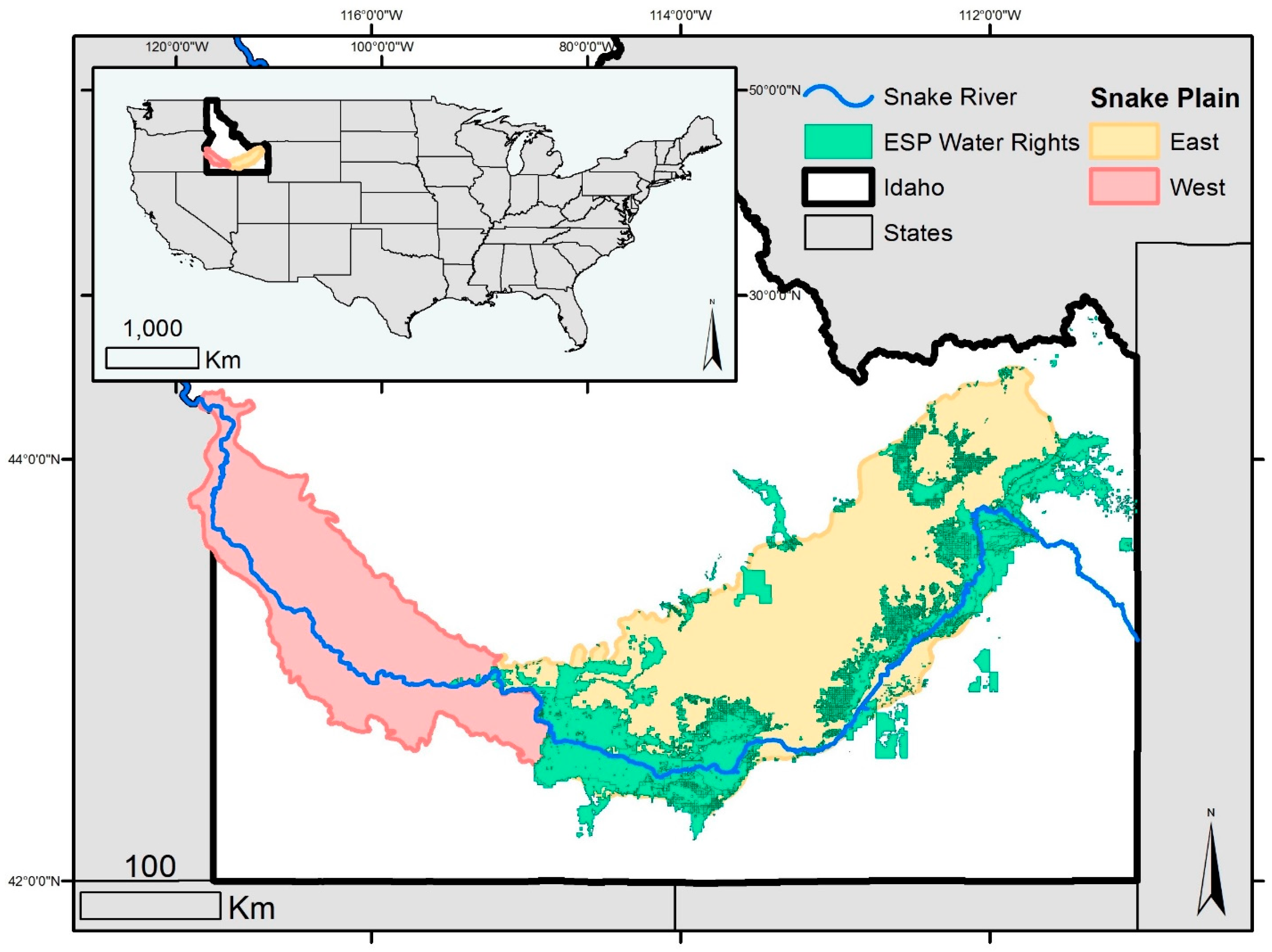
The Snake River Plain, underlain by the Snake Plain Aquifer, spans most of southern Idaho and is home to the majority of the state’s population and agricultural production. The region is approximately 650 km running east to west, with elevations declining from 1680 m above mean sea level in the east to 680 m in the west [25]. Approximately 30% of the Plain’s land area is in agriculture. Undeveloped lands are predominantly covered in shrub and scrub, with pine forests in higher elevation areas [26].
The Plain consists of two portions that are hydrologically distinct with differing aquifers, population densities, and agricultural production (Figure 1). The Eastern Snake River Plain, in yellow, spans the southeastern and southcentral portion of the Plain. This portion of the region runs from the eastern border of the state, near the headwaters of the Snake River in the Teton mountain range, southwest to the Thousand Springs region. The Western Snake River Plain, in pink, spans the remainder of the region from Thousand Springs to the Oregon border. Human population densities in the east are low and agriculture focuses on spring and winter wheat, alfalfa, barley, corn, potatoes, and sugarbeets. The west is home to the Boise City–Nampa Metropolitan Statistical Area and the majority of the state’s population. Much of the agricultural production in the west is located near the Oregon border and includes a diverse set of specialty fruit and vegetable crops, such as onions, mint, viticulture, hops, and orchard fruit [27].
2.1. Climate and Agriculture
The Snake River Plain has a Mediterranean-style arid to semi-arid climate with dry summers. Agriculture in the region relies heavily on supplemental irrigation using surface water from the Snake River and its tributaries and groundwater from the Snake Plain Aquifer. Climate varies across the Plain with the east-to-west gradient in elevation. The highest temperatures and lowest precipitation occur in the west, which has a maximum mean annual temperature of 13 °C and receives an average of 25 cm of precipitation each year. Higher precipitation is observed in the east, where up to 35 cm of precipitation falls on average each year, predominantly during the winter months [28].
The Plain is surrounded by mountains higher than 2800 m in elevation. These mountains receive the majority of the region’s precipitation as winter snowpack, which provides most of the water used for irrigation. Because of a dependence on variable and changing snowpack, the region’s agriculture is especially vulnerable to the effects of climate change [29]. Climate change is expected to result in a decline in snowpack as precipitation events shift from snow to rain and as snowmelt occurs earlier in the spring due to higher temperatures [30,31,32,33,34,35]. Increased variability in flows due to changes in snowpack will introduce uncertainty into agricultural production and is likely to affect the region’s economy, hydrology, and ecology.
Idaho ranks third among states in terms of water withdrawals and first in water withdrawals per capita [36]. The vast majority of water withdrawn in the state is withdrawn in the Snake River Plain, most of which (85.6%) is withdrawn for irrigation [36]. Approximately 60% of the region’s irrigated acres are irrigated with surface water, the remainder with groundwater. The most profitable crops grown in the region can be grown only with supplementary irrigation, including grain corn, beans, and potatoes. Dryland agriculture is feasible in some areas of the region for a subset of crops, including wheat, alfalfa, and pasture. However, yields for these crops are much higher with irrigation. For example, average yield for dryland alfalfa hay was 3.14 metric tons/ha in 2012 compared to 10.31 metric tons/ha when irrigated [27].
2.2. Water Rights
Water is the primary limiting factor for agricultural production in the study region. A large portion of the land with soils suitable for agricultural production is not used [37]. Rather, the extent of agriculture is defined by legal restrictions that govern where and when land may be irrigated. These restrictions take the form of property rights, referred to as water rights, which define the availability of irrigation water for individual farms. Water rights therefore influence crop yields, land-use decisions, and agricultural land values [38,39,40].
Throughout the arid and semi-arid western United States, the doctrine of prior appropriation is used to regulate surface water rights for irrigation. Prior appropriation defines many attributes of water rights, but is best known for its seniority based structure, summarized as “first in time, first in right”. Under this system, every irrigator must have a state-issued water right permitting the withdrawal of water from a specific source. Each water right has a corresponding priority date, defined as the date on which water was first claimed for diversion under the right. The priority date defines a right’s position and precedence within the regional hierarchy of rights. Those established earliest in time are relatively senior and have first claim to available flows. Those established later in time are relatively junior. If there is not sufficient water to satisfy all rights, rights will be curtailed (cut off) starting with the most junior. Thus, relatively junior water rights face the risk of a shortage of water for irrigation, especially during dry growing seasons.
In Idaho, both surface water and groundwater rights are allocated based on prior appropriation doctrine. Every surface water diversion and groundwater well in the region must have a state-issued water right that defines water-use privileges. In addition to the priority date, water rights in Idaho include a specific point of diversion, place of use, maximum rate of water diversion, season of use limitations, and ownership information. These attributes of water rights are fixed in the sense that any change requires a lengthy administrative review by the state and substantial legal costs for the party proposing the change. Even with the appropriate paperwork, substantive changes to water rights, such as a change in the point of diversion, place of use, or maximum rate of diversion, are often denied by the state.
This analysis uses information on the place of use for each water right in the study region, which is recorded as a geographically referenced polygon that defines the land base over which irrigation water may be applied. The place of use definition means that water rights are effectively associated with a specific parcel of land. This feature of the data allows for straightforward geospatial analysis of water rights and water use. The place of use is the means by which the state water agency, the Idaho Department of Water Resources, monitors and enforces water use restrictions. Because the direct monitoring of water diversions is costly and electronic flowmeters are rarely required of agricultural irrigators, the Idaho Department of Water Resources has begun to regulate water rights based on whether the spatial extent of irrigation and/or evapotranspiration exceed water right constraints [41]. It follows that accurate mapping of the extent of irrigation is especially important in this region.
3. Materials and Methods
This study builds on [11], which compared a combination of image classification algorithms and spectral indices to identify irrigated lands in the Snake River Plain for the 2002 and 2007 agricultural growing seasons. This comparison showed that a threshold-based classification approach using the seasonal maximum value for NDMI and Landsat 5 data was preferred among alternatives based on its consistent ability to distinguish irrigated from non-irrigated land. This study extended the analysis of [11] by applying the same classification algorithm to the full Landsat 5–8 time series from 1984–2016.
We conducted the analysis using Google Earth Engine’s API and images from Landsat 5 (1984–2011) and Landsat 8 (2013–2016) all of which were at a 30 m resolution. To avoid introducing erroneous observations caused by the Landsat 7 scan line corrector failure, we substituted 2011 Landsat 5 data for 2012 Landsat 7 data to complete the 1984–2016 time series. We used surface reflectance data sets and performed cloud masking based on Fmask values provided with each dataset [42].
3.1. Image Classification
We implemented a binary image classification method based on the magnitude of the seasonal maximum NDMI value observed at each pixel relative to a threshold that separates irrigated from non-irrigated land. NDMI is defined as:
where represents near infrared reflectance (0.76–0.90 μm) and represents short wave infrared reflectance (1.55–1.75 μm). We defined the growing season as 1 April–31 October, consistent with the typical planting to harvest interval for the study region.
To determine the threshold that distinguishes irrigated and non-irrigated land, we developed a training dataset of 404 known land-use points using manual interpretation of high-resolution aerial photographs from the National Agriculture Imagery Product (NAIP). We selected 10 irrigated and 10 non-irrigated points within each of the 21 counties in the Snake River Plain. In the study region, NAIP images are available only for the 2003, 2004, 2006, and 2009 growing seasons. We selected training points that were consistently irrigated or non-irrigated for all available NAIP images.
We used nine pixel values in a three-by-three square surrounding each training point to calculate an observed value for NDMI based on each available Landsat scene. The presence of irrigation infrastructure, farm equipment, and other anomalies may skew observed values of NDMI and reduce classification accuracy. To account for this effect, we removed any outlier pixels, defined as pixels with NDMI values outside of two standard deviations of the mean for each nine-pixel square. From the resulting set of observations at each training point, we selected the seasonal maximum value of NDMI.
We used these observations of seasonal maximum NDMI to characterize the observed distribution of NDMI values across irrigated and non-irrigated training points. We described the distributions of NDMI seasonal maximums each year using Matlab’s (version 9.2, MathWorks, Natick, MA, USA) kdensity function [43]. We defined the classification threshold for each year as the value for NDMI at which the kernel density functions for irrigated and non-irrigated points intersect. The date on which maximum NDMI occurs varies across years with crop/vegetation, cloud cover, and the date of the satellite pass (since the whole study area is not covered in a single pass). However, the temporal resolution of the Landsat data (2 images per month) is not fine enough to analyze trends in the date of the maximum NDMI value.
3.2. Time Series
Because NAIP imagery does not span the full duration of the Landsat 5–8 time series, we did not know with certainty whether some of our training points transitioned between irrigated and non-irrigated status prior to 2003. This presented a challenge in classification particularly for early years in the time series. We expected this uncertainty in the early status of the training points to result in an increase in the variance of the distributions of NDMI values as we moved further in time from the NAIP time series. To address this challenge, we compared the distribution of NDMI across our sample points for each year to ensure stability within each class over the duration of the time series. We tested several statistical methods to identify outlier and candidate misclassified values in our dataset. We excluded sample points from the analysis if the observed value of NDMI at an irrigated point was within one standard deviation of the mean of the non-irrigated distribution for the years covered by NAIP (and vice versa for non-irrigated points). This method removed the influence of potentially misclassified points for pre-NAIP growing seasons in our time series (1984–2002). This resulted in 8–19% of points removed in the years 1984–1990 and 0–10.5% of points removed in the years 1991–2002.
Our objective in this analysis is to evaluate long-term (decadal) trends in the extent of irrigation. However, year-to-year variation in irrigated land areas introduces noise that obscures longer-term changes. Two- to three-year crop rotations are common in Idaho, but rotations on the order of four to five years with land fallowing are often recommended to minimize pest and disease risks and increase revenue [44]. To evaluate long-term changes in the extent of irrigated area, we identified points in our dataset as irrigated in a given year if the point was classified as irrigated at any time within a five-year window. For example, we compared irrigated area during the period 1984–1989 with irrigated area during the period 2011–2016. If a parcel was irrigated at any point in either window, it was classified as irrigated at the beginning or end of the time series, respectively. A change from non-irrigated to irrigated indicates that there was no irrigation from 1984–1989 and that the same pixel was irrigated at least one year from 2011–2016. We created a map of change in irrigated area by comparing our classification results at these end points of the time series. To remove the risk of false positives within non-agricultural land covers, we masked out only water, barren lands (the study area contains large areas of exposed lava that are highly reflective), forest, and scrublands using the 2006 National Land Cover Database (NLCD) [26]. Agricultural expansion over our time series occurred predominantly on grasslands, while agricultural contraction occurred predominantly on urban lands. For each year, we generate the following time series outputs: the mean and standard deviation of NDMI for irrigated and non-irrigated areas, the mean NDMI across all pixels (irrigated and non-irrigated), the NDMI classification threshold, and total irrigated land area.
3.3. Precipitation
We examined precipitation over the duration of our time series to assess the effect of seasonal water availability on irrigation patterns. Two precipitation datasets were used as a measure of water availability. The first dataset includes gridded (~4 km) values for total precipitation in each irrigation year (beginning and ending 1 October) produced by the National Weather Service for 2006–2016 [45,46]. We replaced missing values in the dataset with the average value in the same irrigation year. The sums of all cell values were then calculated to estimate total precipitation volume for the Snake River Basin watershed [47]. This total for the watershed captures precipitation on the Plain itself as well as precipitation falling during winter in surrounding mountainous areas. Precipitation stored as mountain snowpack melts off and fills reservoirs and surface waterways that support irrigation throughout drier portions of the growing season. In addition, we included data describing precipitation directly on the Plain. This measure does not capture precipitation in surrounding mountainous areas, but has the advantage that it covers a longer time series than the gridded dataset. We used data from a centrally located rain gauge in Jerome, Idaho that spans the years 1985–2016. From these data, we generated scatterplots and calculated the coefficient of determination (R2) between the precipitation variables and our time series outputs.
3.4. Water Rights in the Eastern Snake River Plain
In this analysis, we are interested in understanding how trends in irrigated land area over time differ across land that is irrigated under different types of water rights. To do so, we use the place of use polygons for each water right, which are linked with data describing all other water rights attributes. In many instances, the polygons defining the place of use for each water right overlap with one another. Overlap indicates that a farmer owns a water right portfolio that permits irrigation of the same parcel of land with rights that have different attributes [40]. To distinguish lands eligible to be irrigated under multiple water rights, we created a new layer describing distinct place of use polygons that are defined by the intersection of places of use. Each revised polygon is defined by a unique combination of overlapping water rights and water rights attributes. These revised water rights combinations were used to calculate the percent area that was irrigated for groundwater, mixed source, and surface water rights each year in the time series.
4. Results
Given the long duration of the time series (33 years), it is not possible to fully display the results of the annual irrigated/non-irrigated classification here. Instead, we describe our time series outputs (Figure 2) and a long-run map of changes in irrigated lands between the ends of the time series (Figure 3). We also present an analysis of the two-way correlation between our time series outputs and precipitation (Figure 4) or water rights attributes (Figure 5). We validated the classification at the pixel scale following the methods in [11]. We created a sample dataset of 150 randomly selected points in the region that were consistently irrigated or non-irrigated for years covered by NAIP. For those years, the classification method consistently produced an overall accuracy on the order of 98%, a producer’s accuracy greater than 96%, a user’s accuracy of 100%, and a kappa value greater than 0.96.
4.1. Time Series
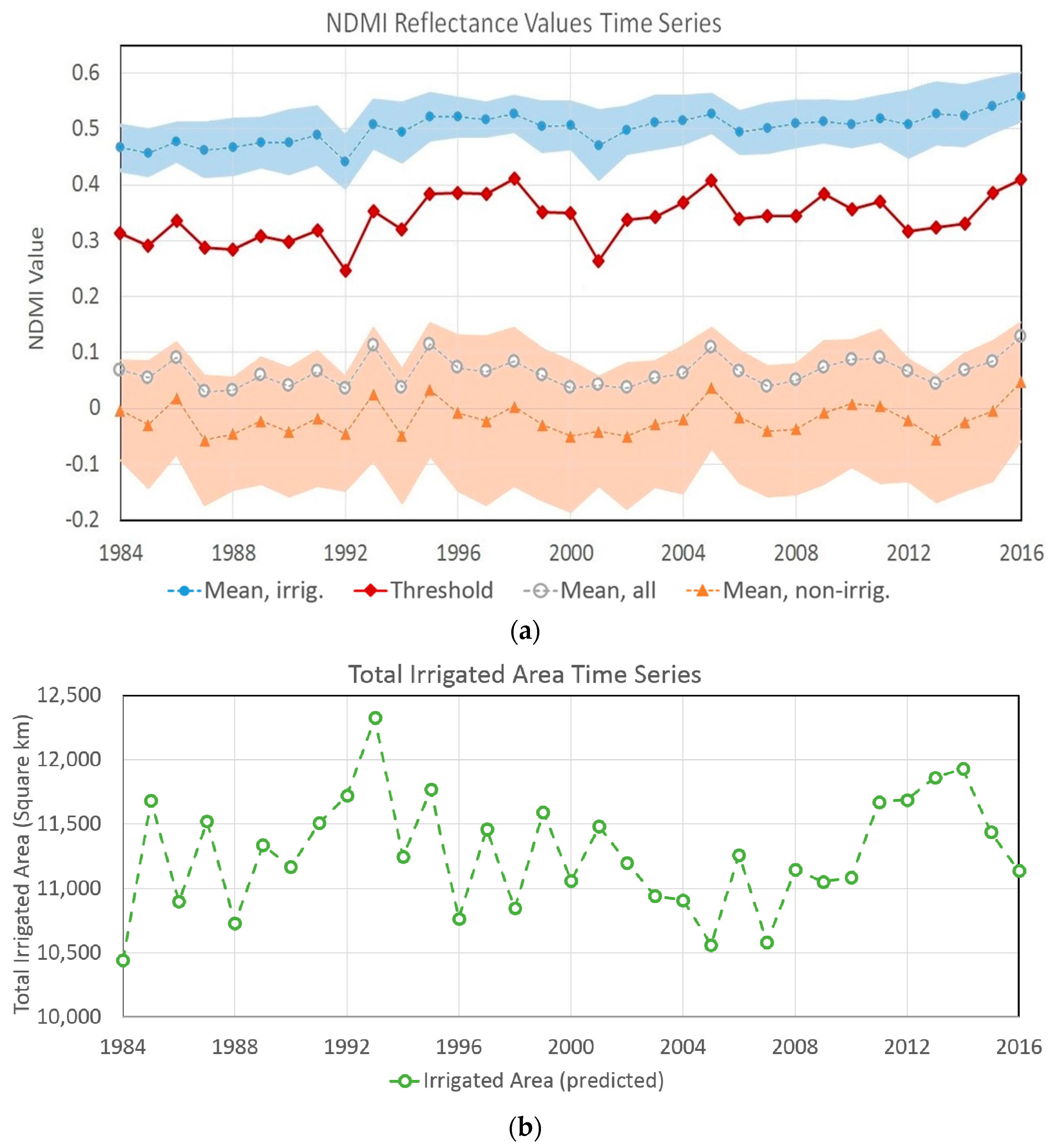
Figure 2a presents the time series of NDMI values, including mean NDMI across all pixels and NDMI values broken out separately for irrigated and non-irrigated pixels. The NDMI values for irrigated pixels (in blue) showed a statistically significant increasing trend over the time series. NDMI values for all pixels and for non-irrigated pixels varied year-to-year, but remained relatively constant over time with no significant long-term trend. The standard deviation in NDMI values for the irrigated class was approximately half the magnitude of that for the non-irrigated class. This follows from the fact that the use of irrigation supports more homogeneous crop productivity and greenness throughout the growing season than dryland agriculture. Figure 2a also shows the annual threshold value of NDMI used to distinguish irrigated from non-irrigated pixels. The threshold value used in image classification increased over time with NDMI values in the irrigated class.
Figure 2b illustrates total irrigated land area for each year in the time series. Total irrigated land area fluctuated between 10,450 km2 (1984) and 12,330 km2 (1993). Across years, the mean and standard deviation for irrigated areas were 11,280 km2 and 432 km2, respectively. Large interannual changes in irrigated land area are likely due to a combination of factors including land fallowing practices and classification error. Comparing Figure 2a,b suggests little correlation between NDMI values of irrigated pixels and irrigated land area. For example, NDMI values declined in 1992 and 2002, but irrigated land area in the same years was close to its long-term mean. The pairwise correlation between the threshold value and irrigated land area was also weak: the R2 for irrigated area and the threshold value was 0.06 for the region. If our choice of index value in the classification drove variation in irrigated land area, we would expect to see a correlation between these two values over the time series. The absence of a correlation suggests that annual variation in irrigated land area was not driven by the index value we chose for use in the classification. This lack of correlation lends support to the accuracy and objectivity of our classification methodology.
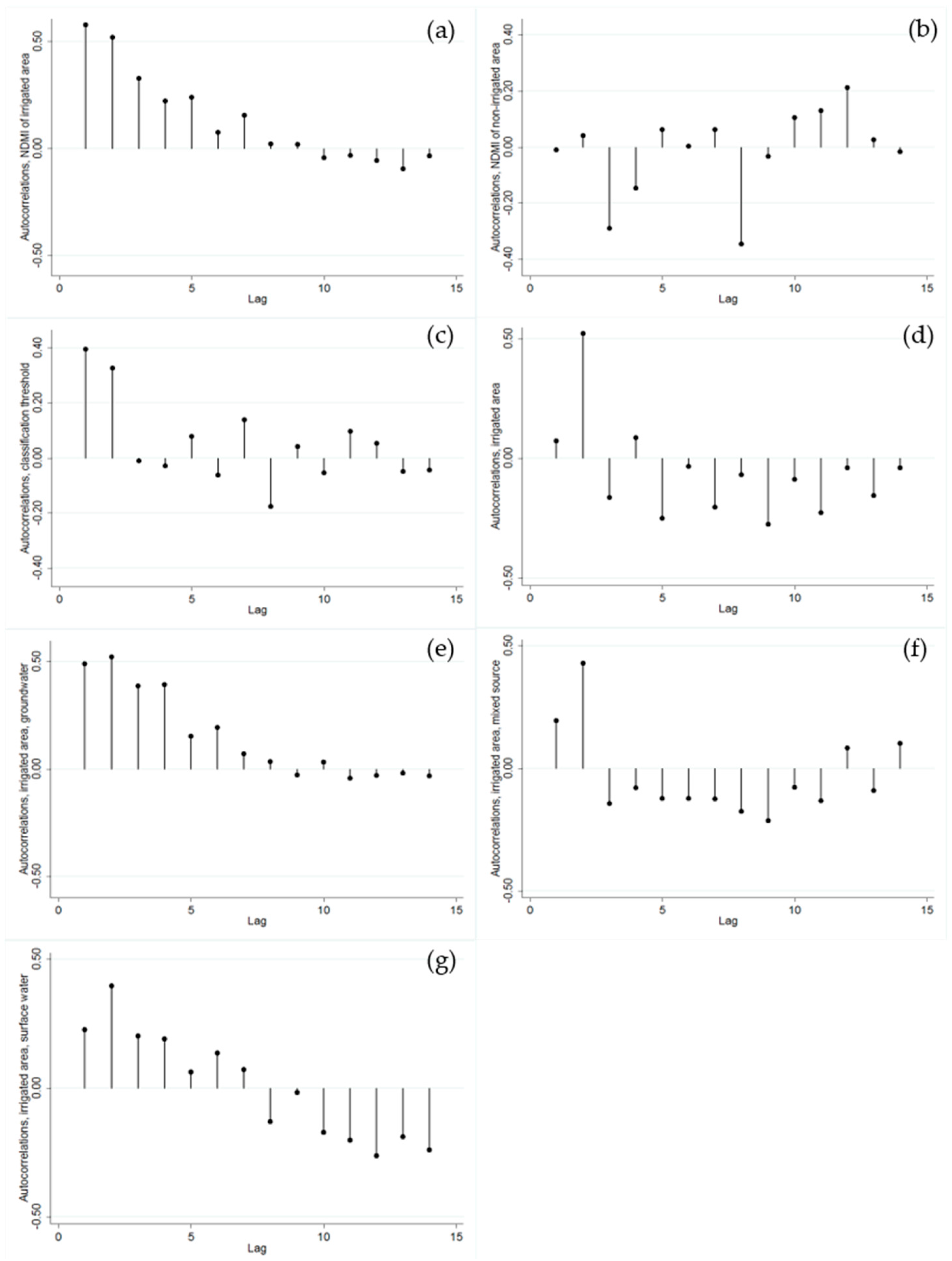
Table A1 in the Appendix presents autocorrelation and Q-statistics for each of the time series plots in Figure 2a,b. Serial correlation is present at up to 10 lags in the NDMI of irrigated areas, but there is little evidence of serial correlation in the NDMI of non-irrigated areas. Weaker serial correlation is present in the time series for the classification threshold and irrigated area. Table A3 in the Appendix presents the results of a linear regression with a time trend for each time series, as well as the Dickey–Fuller test statistic of the null hypothesis that each series is a random walk with drift (versus the alternative of a stationary series around a linear time trend). For all time series, we reject the null hypothesis of a unit root. Consistent with visual inspection of Figure 2a,b, the linear trend for the NDMI of irrigated areas and the classification threshold is positive and highly statistically significant. Figure A1 illustrates the autocorrelation coefficients for each time series. Those for NDMI of irrigated areas, Figure A1a, and the classification threshold, Figure A1c, most closely resemble an AR(1) process. This is consistent with the time series regression results presented in Table A4.
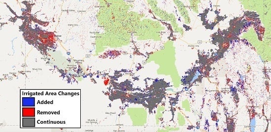
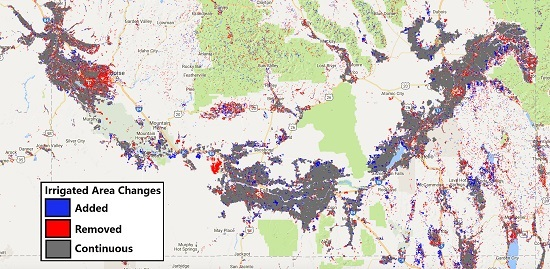
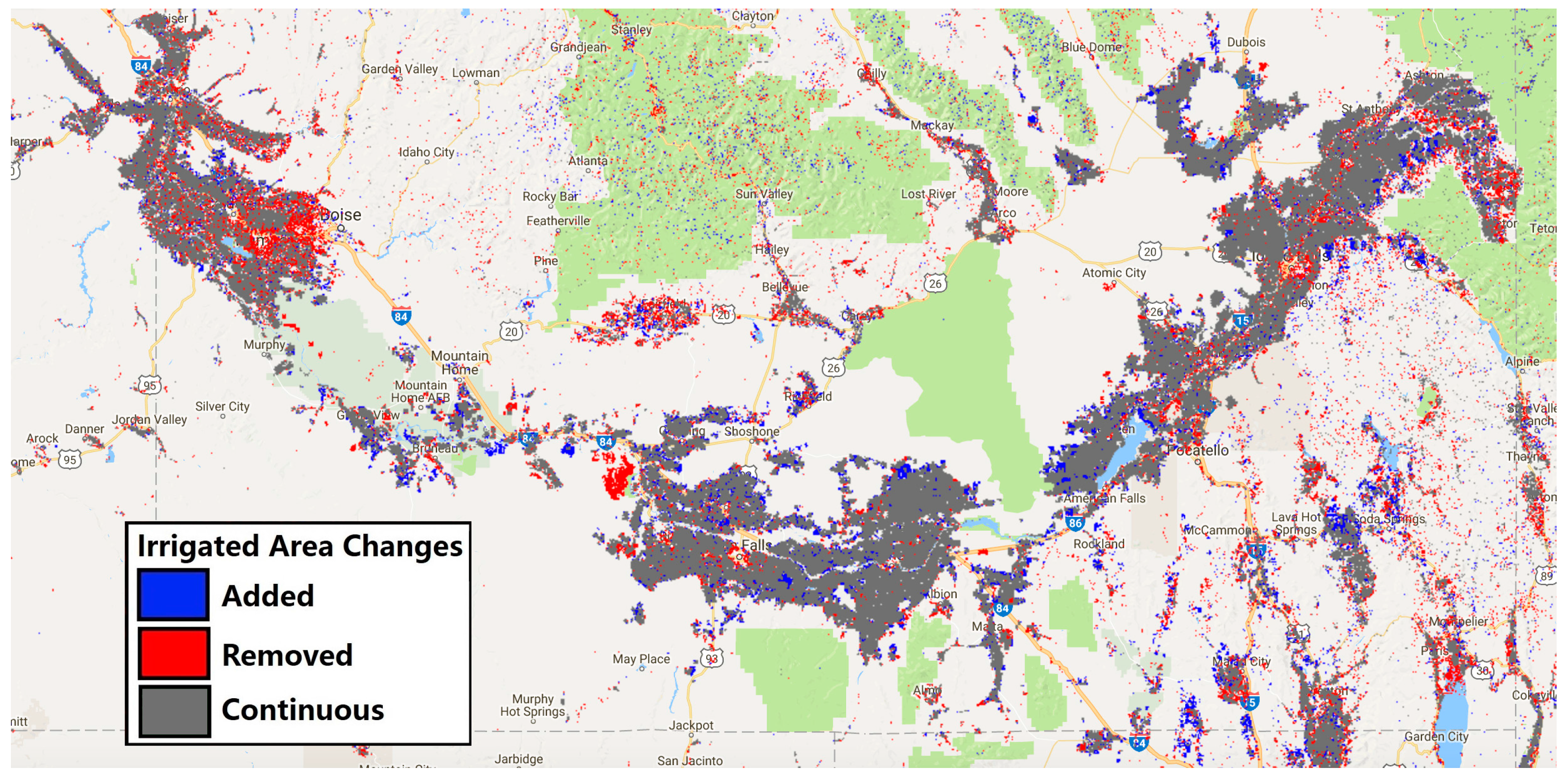
Figure 3 presents a map of long-term change in irrigated area for the study region. Pixels in green are those for which irrigated status was constant over the time series. These pixels accounted for the majority of the irrigated landscape in the study region. Pixels converted from non-irrigated to irrigated (blue) were scattered throughout the Eastern Snake River Plain. These pixels were predominantly located on the perimeter of continuously irrigated area and indicate an expansion in irrigated agriculture. Pixels converted from irrigated to non-irrigated (red) were located primarily in the vicinity of urban areas in the study region. For example, the large red area in the northwest portion of the study region near Boise (the state capital) was the result of urban and suburban expansion into agricultural areas. The largest contiguous area of red pixels, near the center of Figure 3, was formerly the site of the Bell Rapids Irrigation District. This land was deliberately removed from irrigated agriculture in 2004 to prevent landslides in the nearby Hagerman Fossil Beds National Monument, which is home to American Indian cultural sites and several endangered species [48].
4.2. Precipitation
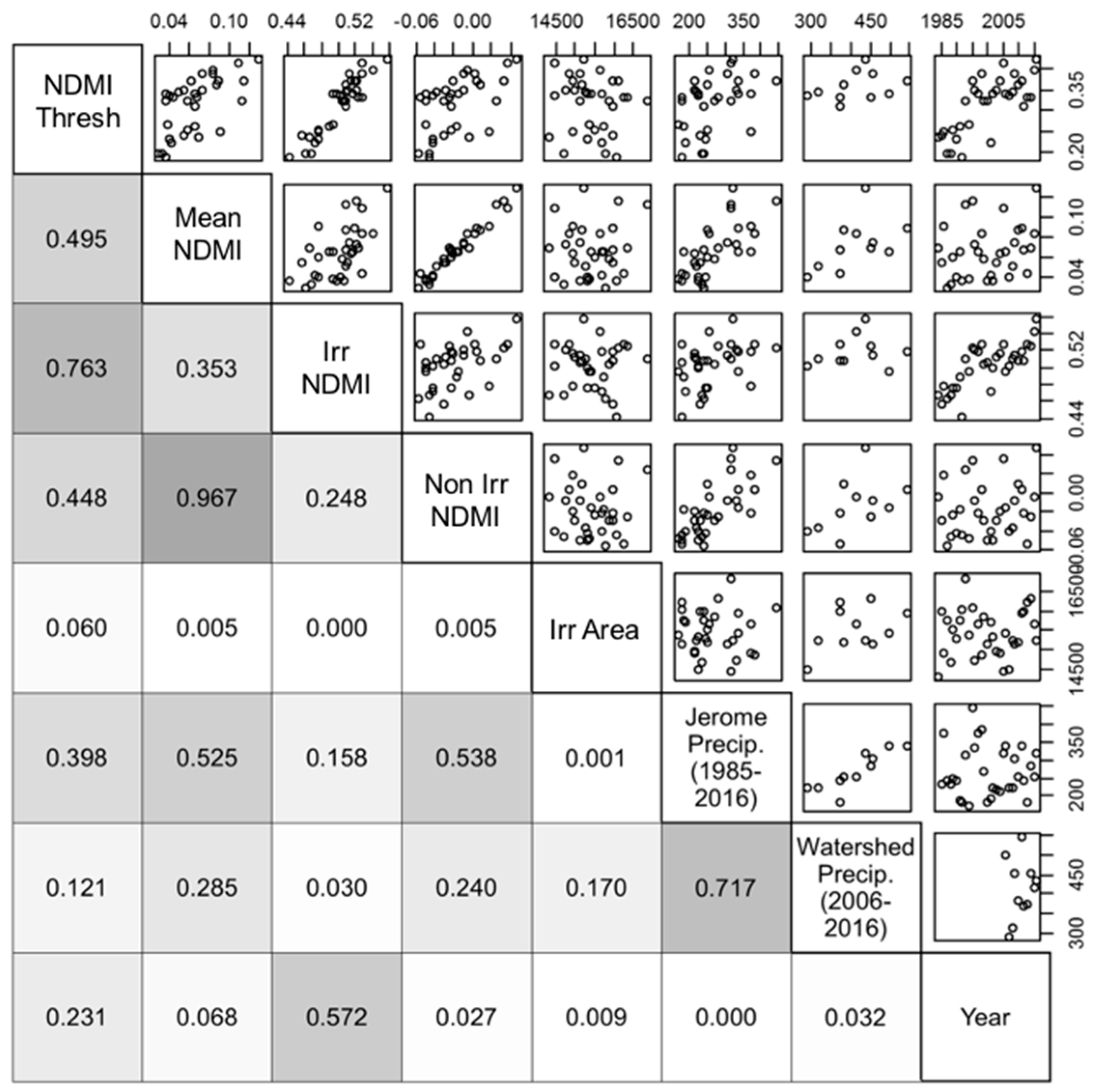
A logical question that arises concerns which factors influence the extent of irrigated land area. We first considered whether precipitation drove changes in irrigated area on an annual or decadal basis. Figure 4 presents R2 values that describe the proportion of variation in our time series that is attributable to the two measures of precipitation.
Figure 4 illustrates pairwise scatterplots (upper right) and R2 values (lower left) for each outcome variable and precipitation measure. In general, the threshold value of NDMI used in classification was correlated with both measures of precipitation, though the correlation was stronger for precipitation measured in Jerome than it was for the watershed as a whole. This may be because the data record at Jerome is longer, or it may be because the greenness of non-irrigated areas was more heavily influenced by direct precipitation on the Plain than by precipitation in adjacent mountainous areas.
Across outcome variables, precipitation was most strongly related to mean NDMI across all pixels and mean NDMI for non-irrigated pixels. The R2 for Jerome precipitation and these two variables was on the order of 0.53–0.54. The relationship between these NDMI values and precipitation throughout the watershed was weaker, with an R2 of 0.24–0.29. Neither precipitation measure was strongly correlated with mean NDMI values for irrigated pixels. This is logical given that irrigation protects farmers from variability in precipitation by sustaining crop productivity throughout dry periods, whereas non-irrigated agricultural production is dependent on precipitation. This result also implies that greenness in irrigated areas was not strongly influenced by precipitation during the growing season, regardless of whether it fell in the mountains or on the Plain.
The relationship between total irrigated land area and precipitation in Jerome was close to zero, and weak for watershed precipitation (an R2 of 0.17). While natural water availability during the growing season exerts some influence on the extent of irrigated agriculture, there are likely more important factors that drive changes in the use of irrigation.
4.3. Water Rights in the Eastern Snake River Plain
Water rights play a key role in determining which irrigated fields receive water and when during a growing season. From Figure 3, there was no clear spatial correlation between the distribution of water rights and the expansion or contraction of irrigated land. To evaluate in greater detail how the extent of irrigated agriculture varies among farms with different types of water rights, we examined the correlation between our five outcome variables and two important water rights attributes—size of the place of use and the water source.
For each water right polygon, we identified the places of use with a large change in the extent of irrigated land area over the time series. We defined a large change as greater than a 25% expansion or contraction of irrigated land between the period 1984–1989 and the period 2011–2016. We compared the characteristics of parcels experiencing large changes with others that have less substantial or no change in irrigated land area.
We found that rights with a large decrease in irrigated area (over a 25% contraction) were disproportionately likely to be surface water rights, whereas those with a large increase in irrigated area (over a 25% expansion) were disproportionately likely to be groundwater rights. In addition, there was greater change in irrigated area among the population of parcels with access to groundwater. For example, 36% of all groundwater rights experienced a large gain in irrigated area, while 16% experienced a large loss. Among surface water rights, 7.6% experienced a large reduction in irrigated area, as opposed to 4.7% that experienced a large gain.
While water source was correlated with large changes in irrigated extent, the correlation between the size of the water right place of use and change in irrigated area was far more pronounced. On average, water right places of use were 204.0 ha. Those with a large reduction in irrigated area were 19.3 ha on average, while those with large increases in irrigated area were an order of magnitude larger with a mean of 120.2 ha.
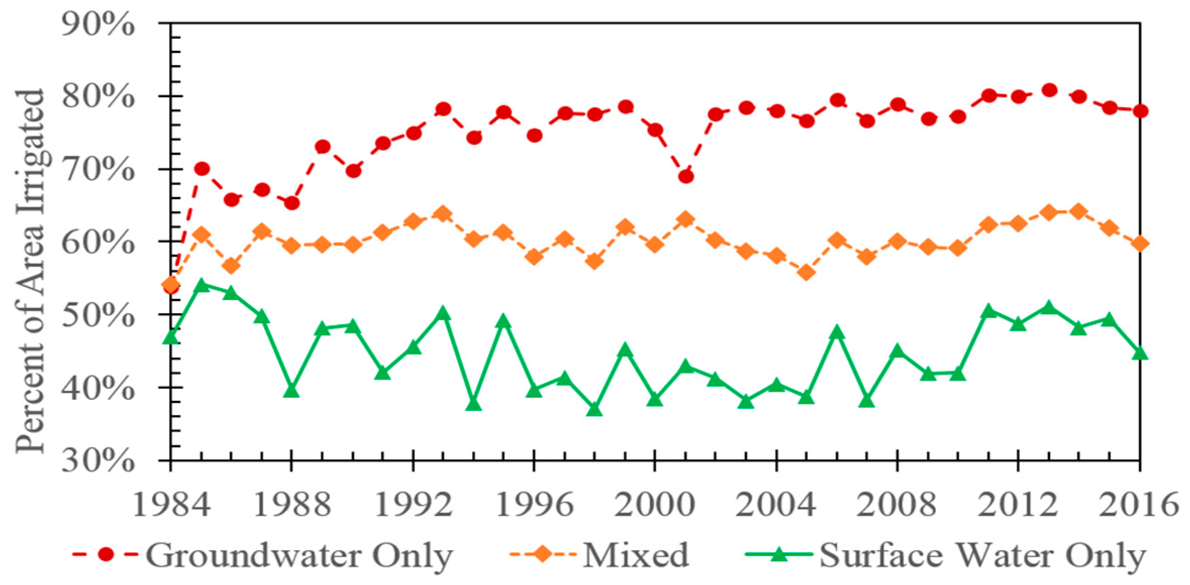
Figure 5 presents a time series of the proportion of the area within each water right that was irrigated each year. We broke the time series out by water rights irrigated only with groundwater, those irrigated only with surface water, and those irrigated with both. Water rights with access to both sources exhibited the least variation on an annual basis, with a standard deviation of 2.3% over the duration of the time series. Variation in irrigated extent for parcels with access to groundwater was nominally higher than that for farms with mixed water sources. Surface water rights had the greatest variability in irrigated area, which was driven by seasonal variability in water inflows.
Figure 5 illustrates that groundwater-dependent farms showed the greatest upward trend in irrigated area over the time series. The portion of the total area irrigated with groundwater increased at a rate of approximately 15 km2 per year over the time series with an R2 of 0.54. This was attributable in part to the fact that the Idaho Department of Water Resources continued approving new groundwater rights into the early 1990s. The dip in area irrigated by groundwater in 2001 corresponded to a one-year program in which Idaho Power Company paid irrigators to reduce power consumption for groundwater pumping [49].
Table A2 in the Appendix presents autocorrelation and Q-statistics for each of the time series plots in Figure 5. Serial correlation is present at up to 10 lags in the area irrigated with groundwater. Weaker serial correlation is present in the time series for area irrigated with mixed water sources or surface water. Table A3 presents the results of a linear regression with a time trend for each time series, as well as the Dickey–Fuller test statistic of the null hypothesis that each series is a random walk with drift (versus the alternative of a stationary series around a linear time trend). For all time series in Figure 5, we reject the null hypothesis of a unit root. Consistent with visual inspection of Figure 5, the linear trend for area irrigated with groundwater is positive and highly statistically significant. Figure A1 illustrates the autocorrelation coefficients for each time series. The autocorrelation coefficients for area irrigated with groundwater, illustrated by Figure A1e, most closely resemble an AR(1) process. This is consistent with the time series regression results presented in Table A3.
5. Discussion
Only the threshold NDMI value and the mean NDMI values on irrigated lands exhibited trends over the duration of the multi-decadal Landsat 5–8 time series. Increasing NDMI values on irrigated lands were likely the result of widespread changes in irrigation practices in the region, which included a shift away from flood irrigation and towards center pivot irrigation. This change in irrigation application methods resulted in increased vegetative growth, higher plant water content, lower water stress, and increased NDMI values [50]. Other developments in crop productivity, herbicides and pesticides, as well as changes in crop selection and management practices also could have contributed to an increase in plant water content and NDMI values.
While the cause for these observed increases in NDMI values cannot be definitively determined, the fact that irrigated land area has no time trend indicates that it was not an artifact of our classification approach and threshold values. If threshold values drove increased NDMI values on irrigated land, we would expect to see a decline in irrigated land area over time (assuming the true irrigated land area is relatively constant) as the upward shift in the threshold value would have caused more irrigated pixels to be misclassified as non-irrigated.
Because the extent of irrigation is regulated by the state of Idaho and relatively few additional water rights were granted during our time series, it is reasonable that the extent of irrigated land area was fairly constant over time. Although seasonal fluctuations in irrigation extent could be partially a result of classification or imaging errors, there were other outside drivers of these changes such as water availability, market conditions, heat, and other factors not considered in this analysis. While the overall extent of irrigation varied, it did not change in any discernable pattern over time. If examined at the scale of the individual irrigator, there may have been more discernable drivers of change, such as changes in specific water allocations or crop selection.
Within existing water rights, the intensity of irrigation (as measured by mean NDMI) was relatively uniform, but there were differences in the extent of irrigation based on water source (groundwater vs. surface water). This was likely a product of Idaho’s water management structure where most irrigators have access to groundwater, and often no meaningful limits are placed on groundwater pumping. We also found that the size of a water right was correlated with the extent of irrigated land area, which affects the viability of heterogeneous farms. Specifically, small water rights were most likely to have lost a large portion of irrigated area over the time series. Larger farms (with larger water rights) were likely to be more viable over the long run. This was likely because larger farms can take advantage of economies of scale; they generally have access to more capital and better equipment; and they may be better able to diversify their crop mix, insulating themselves from losses due to pests or market variability. Looking forward, smaller water rights owners may be less able to compete with larger farms and face an increased risk of exiting the industry over the long run [51,52]. This is part of an ongoing trend in the U.S. and other developed countries, in which agriculture is shifting away from small family farms towards larger industrial farms [53,54].
5.1. Sources of Uncertainty
Likely the largest source of error in this study was the training dataset. Corrections were made to account for limitations in its accuracy, but the effectiveness of these corrections cannot be precisely quantified. The study in [11] evaluated the error of this methodology for two years (2002 and 2007) and found a pixel scale overall accuracy of 98.0–98.7%, an R2 of 0.970–0.981 for irrigated land area per county, and a root mean square error (RMSE) of 45–66 square kilometers. The area errors were reduced slightly by the inclusion of NLCD masking in this study (R2 of 0.975–0.985 and RMSE of 45–53 km2). However, it is likely that older datasets were less accurate due primarily to shifts in land use at the points in the training dataset. Differences in the Landsat sensors, image timing, the date on which maximum NDMI is observed, and cloud cover all have potential impacts on classification accuracy. Additionally, on-the-ground changes in agricultural practices such as irrigation methods (shifts towards center pivot irrigation and away from flood irrigation), predominant crop type, pest management, and crop improvement could have contributed to classification errors since these practices could result in different NDMI values over time. Without additional training data, it is not possible to quantify the extent to which our measured shifts over time in classification values (and the upward trend in NDMI values on irrigated lands) were a result of real changes versus classification error.
Precipitation events during the growing season likely contributed to seasonal variability in our results, affecting the NDMI values of irrigated and non-irrigated pixels. Additionally, geographically isolated precipitation events could have caused some non-irrigated points to be misclassified as irrigated in those areas. Although we examined precipitation in this study, we did not directly account for differences in precipitation amounts across the study region in the calculation of each threshold. Inclusion of such precipitation data could allow for a higher degree of classification accuracy, and potentially make this methodology more widely applicable to regions that receive more precipitation during the growing season.
5.2. Opportunities for Future Research
Climate change has the potential to destabilize water supplies in the Snake River Plain and other regions worldwide. The results and the datasets developed by this study could be used to assess and predict the impacts of climate change on land-use decision-making [40]. More detailed econometric modeling of irrigator behavior within the study region, which accounts for omitted factors such as temperature, agricultural market forces, and productivity, may be possible based on the results of this study. Such modeling could be used to predict responses to various climate change scenarios and to provide the basis for developing new policies that efficiently balance water conservation and agricultural production in irrigated regions. Additionally, because our analysis was performed using Google Earth Engine, it is easily scalable and transferrable to other regions of the world (see Supplementary Materials for source code). This makes it possible for future research to apply our methods to assess policy decisions in other locations and to compare the impacts that differences in policy across regions have on irrigation practices.
6. Conclusions
In the face of increased competition for water resources, understanding irrigator responses to changes in water availability is vital to building effective and efficient water policy and management strategies. In this analysis, we used remotely sensed data from the Landsat time series to evaluate trends in irrigated areas within the Snake River Plain over 33 years. A wealth of data is available in the Landsat archives, but translating those images into land use/land cover information is often limited by the availability of adequate training data. While new cloud computing platforms such as the Google Earth Engine allow us to access and process huge volumes of data with relative ease, we are still limited by our ability to interpret this data. This study presents a novel approach to classify irrigated lands during a period predating our training dataset. Furthermore, this paper contributes to a growing body of remote sensing studies that find that, by applying simple statistics such as the median, maximum, or minimum to multi-temporal data, we can reliably map a wide variety of land cover regimes [55,56,57,58]. These techniques have the potential to become more commonplace as high performance cloud computing allows easier access to multi-temporal data and as more data becomes available through the Sentinel program.
We found that the extent of irrigated area fluctuated on an annual basis, but remained fairly constant across decades. However, within classes of irrigators, we demonstrated that there were substantial differences in irrigation changes over time. Smaller irrigators and those who relied on surface water were most likely to lose irrigated area over the period of record. Conversely, larger irrigators who relied on groundwater were most likely to see an expansion in irrigated area. This expansion in groundwater-irrigated area was robust even to a regional-scale, annual effort to reduce groundwater pumping [49].
Supplementary Materials
The following is available online at www.mdpi.com/2072-4292/10/1/145/s1. The source code for our analysis within Google Earth Engine is available at https://github.com/ericwchance/Irrigation_Extent_Time_Series. Video S1: Video time series of irrigated land area in the Snake River Plain.
Acknowledgments
Support for this paper was provided by the NASA Land Cover/Land Use Change Program under award NNX14AH15G, a Junior Faculty Award from the Virginia Tech Institute for Critical Technology and Applied Science, and the McIntire–Stennis Cooperative Forestry Research Program.
Author Contributions
All authors took part in the conception of and designed the study. E.K.C. performed the experiments and analyzed the data. K.M.C. conducted the time series analysis. E.K.C., K.M.C., and V.A.T. drafted the manuscript. K.M.C. and V.A.T. revised the manuscript and managed this research.
Conflicts of Interest
The authors declare no conflict of interest. The funding sponsors had no role in the design of the study; in the collection, analyses, or interpretation of data; in the writing of the manuscript, and in the decision to publish the results.
Appendix A

Table A1.
Autocorrelation and Q-statistics, time series in Figure 2.
Table A1.
Autocorrelation and Q-statistics, time series in Figure 2.
| Lag | Autocorrelation | Q (p-Value) | Autocorrelation | Q (p-Value) | ||
|---|---|---|---|---|---|---|
| NDMI of Irrigated Areas | NDMI of Non-Irrigated Areas | |||||
| 1 | 0.576 | 11.98 | (0.001) | −0.011 | 0.00 | (0.947) |
| 2 | 0.519 | 22.01 | (0.000) | 0.040 | 0.07 | (0.968) |
| 3 | 0.326 | 26.11 | (0.000) | −0.290 | 3.30 | (0.347) |
| 4 | 0.220 | 28.04 | (0.000) | −0.148 | 4.17 | (0.384) |
| 5 | 0.238 | 30.39 | (0.000) | 0.062 | 4.33 | (0.503) |
| 6 | 0.075 | 30.62 | (0.000) | 0.003 | 4.33 | (0.632) |
| 7 | 0.155 | 31.69 | (0.000) | 0.061 | 4.50 | (0.721) |
| 8 | 0.022 | 31.71 | (0.000) | −0.345 | 9.98 | (0.266) |
| 9 | 0.019 | 31.73 | (0.000) | −0.033 | 10.04 | (0.348) |
| 10 | −0.045 | 31.83 | (0.000) | 0.105 | 10.59 | (0.391) |
| Classification threshold | Irrigated area | |||||
| 1 | 0.395 | 5.64 | (0.018) | 0.073 | 0.19 | (0.663) |
| 2 | 0.326 | 9.60 | (0.008) | 0.520 | 10.26 | (0.006) |
| 3 | −0.011 | 9.60 | (0.022) | −0.165 | 11.31 | (0.010) |
| 4 | −0.029 | 9.63 | (0.047) | 0.085 | 11.60 | (0.021) |
| 5 | 0.079 | 9.89 | (0.078) | −0.250 | 14.17 | (0.015) |
| 6 | −0.063 | 10.06 | (0.122) | −0.034 | 14.22 | (0.027) |
| 7 | 0.139 | 10.91 | (0.143) | −0.204 | 16.07 | (0.025) |
| 8 | −0.176 | 12.34 | (0.137) | −0.069 | 16.29 | (0.039) |
| 9 | 0.042 | 12.43 | (0.190) | −0.277 | 19.97 | (0.018) |
| 10 | −0.055 | 12.58 | (0.248) | −0.088 | 20.36 | (0.026) |
Notes: NDMI is the Normalized Difference Moisture Index.
Table A2.
Autocorrelation and Q-statistics, time series in Figure 5.
Table A2.
Autocorrelation and Q-statistics, time series in Figure 5.
| Lag | Autocorr. | Q (p-Value) | Autocorr. | Q (p-Value) | Autocorr. | Q (p-Value) | |||
|---|---|---|---|---|---|---|---|---|---|
| Irrigated Area, Groundwater | Irrigated Area, Mixed | Irrigated Area, Surface Water | |||||||
| 1 | 0.488 | 8.60 | (0.003) | 0.195 | 1.36 | (0.243) | 0.226 | 1.84 | (0.175) |
| 2 | 0.521 | 18.71 | (0.000) | 0.429 | 8.24 | (0.016) | 0.396 | 7.67 | (0.022) |
| 3 | 0.386 | 24.45 | (0.000) | −0.144 | 9.03 | (0.029) | 0.201 | 9.23 | (0.026) |
| 4 | 0.391 | 30.55 | (0.000) | −0.080 | 9.29 | (0.054) | 0.190 | 10.67 | (0.031) |
| 5 | 0.153 | 31.51 | (0.000) | −0.124 | 9.93 | (0.077) | 0.062 | 10.83 | (0.055) |
| 6 | 0.192 | 33.08 | (0.000) | −0.124 | 10.58 | (0.102) | 0.135 | 11.60 | (0.071) |
| 7 | 0.069 | 33.30 | (0.000) | −0.125 | 11.27 | (0.127) | 0.071 | 11.83 | (0.106) |
| 8 | 0.033 | 33.35 | (0.000) | −0.177 | 12.72 | (0.122) | −0.131 | 12.62 | (0.126) |
| 9 | −0.030 | 33.39 | (0.000) | −0.215 | 14.94 | (0.093) | −0.018 | 12.64 | (0.180) |
| 10 | 0.030 | 33.44 | (0.000) | −0.079 | 15.25 | (0.123) | −0.173 | 14.13 | (0.167) |
Table A3.
Regression results, all time series.
| Time Series | Trend Coeff. (p-Value) | Dickey–Fuller Test Statistic (p-Value) | |
|---|---|---|---|
| NDMI of irrigated areas | 0.002050 (0.000) | −4.053 (0.007) | |
| NDMI of non-irrigated areas | 0.000474 (0.365) | −5.134 (0.000) | |
| Classification threshold | 0.002054 (0.005) | −3.975 (0.010) | |
| Irrigated area | 4.492831 (0.582) | −5.274 (0.000) | |
| Irrigated area, groundwater | 0.004339 (0.000) | −6.335 (0.000) | |
| Irrigated area, mixed | 0.000653 (0.130) | −4.974 (0.000) | |
| Irrigated area, surface water | −0.000560 (0.545) | −4.317 (0.003) | |
Notes: NDMI is the Normalized Difference Moisture Index. For each time series, estimated coefficient for a linear time trend is from a linear regression model of the form: , where . The Dickey–Fuller test statistic includes a linear time trend. p-values are in parentheses.
Table A4.
AR(1) regression results, all time series.
| Time Series | Log-Likelihood | Estimates (p-Value) | ||
|---|---|---|---|---|
| Constant Coeff. | AR(1) Coeff. | Sigma | ||
| NDMI of irrigated areas | 82.354 | 0.5028 (0.000) | 0.6913 (0.000) | 0.0198 (0.000) |
| NDMI of non-irrigated areas | 71.515 | −0.0180 (0.001) | −0.0132 (0.952) | 0.0277 (0.000) |
| Classification threshold | 61.847 | 0.3419 (0.000) | 0.4256 (0.015) | 0.0370 (0.000) |
| Irrigated area | −246.886 | 11271.78 (0.000) | 0.0797 (0.735) | 429.38 (0.000) |
| Irrigated area, groundwater | 57.012 | 0.7311 (0.000) | 0.8085 (0.000) | 0.0423 (0.000) |
| Irrigated area, mixed | 78.316 | 0.6011 (0.000) | 0.2390 (0.222) | 0.0225 (0.000) |
| Irrigated area, surface water | 53.704 | 0.4478 (0.000) | 0.2203 (0.233) | 0.0475 (0.000) |
Notes: NDMI is the Normalized Difference Moisture Index. Sigma is the estimated standard deviation of the white-noise disturbance.
Figure A1.
Time series autocorrelation coefficients up to 14 lags for: (a) Normalized Difference Moisture Index (NDMI) of irrigated areas; (b) NDMI of non-irrigated areas; (c) classification threshold; (d) irrigated area; (e) irrigated area, groundwater only; (f) irrigated area, mixed source; and (g) irrigated area, surface water only. (a–d) are for time series from Figure 2; (e–g) are for time series from Figure 5.

References
- Carleton, T.A.; Hsiang, S.M. Social and economic impacts of climate. Science 2016, 353, aad9837. [Google Scholar] [CrossRef] [PubMed]
- McDonald, R.I.; Girvetz, E.H. Two challenges for US irrigation due to climate change: Increasing irrigated area in wet states and increasing irrigation rates in dry states. PLoS ONE 2013, 8, e65589. [Google Scholar] [CrossRef] [PubMed]
- Mehta, V.K.; Haden, V.R.; Joyce, B.A.; Purkey, D.R.; Jackson, L.E. Irrigation demand and supply, given projections of climate and land-use change, in Yolo County, California. Agric. Water Manag. 2013, 117, 70–82. [Google Scholar] [CrossRef]
- Niles, M.T.; Lubell, M.; Brown, M. How limiting factors drive agricultural adaptation to climate change. Agric. Ecosyst. Environ. 2015, 200, 178–185. [Google Scholar] [CrossRef]
- Schlenker, W.; Hanemann, W.M.; Fisher, A.C. Water availability, degree days, and the potential impact of climate change on irrigated agriculture in California. Clim. Chang. 2007, 81, 19–38. [Google Scholar] [CrossRef]
- Allen, R.G.; Tasumi, M.; Morse, A.; Trezza, R. A Landsat-based energy balance and evapotranspiration model in western U.S. water rights regulation and planning. Irrig. Drain. Syst. 2005, 19, 251–268. [Google Scholar] [CrossRef]
- Bastiaanssen, W.G.M.; Noordman, E.J.M.; Pelgrum, H.; Davids, G.; Thoreson, B.P.; Allen, R.G. SEBAL model with remotely sensed data to improve water-resources management under actual field conditions. J. Irrig. Drain. Eng. 2005, 131, 85–93. [Google Scholar] [CrossRef]
- Folhes, M.T.; Renno, C.D.; Soares, J.V. Remote sensing for irrigation water management in the semi-arid Northeast of Brazil. Agric. Water Manag. 2009, 96, 1398–1408. [Google Scholar] [CrossRef]
- Ozdogan, M.; Woodcock, C.E.; Salvucci, G.D.; Demir, H. Changes in summer irrigated crop area and water use in Southeastern Turkey from 1993 to 2002: Implications for current and future water resources. Water Resour. Manag. 2006, 20, 467–488. [Google Scholar] [CrossRef]
- Biggs, T.W.; Thenkabail, P.; Gumma, M.K.; Scott, C.A.; Parthasaradhi, G.; Turral, H. Irrigated area mapping in heterogeneous landscapes with MODIS time series, ground truth and census data, Krishna Basin, India. Int. J. Remote Sens. 2006, 27, 4245–4266. [Google Scholar] [CrossRef]
- Chance, E.W.; Cobourn, K.M.; Thomas, V.A.; Dawson, B.C.; Flores, A.N. Identifying irrigated areas in the Snake River Plain, Idaho: Evaluating performance across compositing algorithms, spectral indices, and sensors. Remote Sens. 2017, 9, 546. [Google Scholar] [CrossRef]
- Draeger, W.C. Monitoring irrigated land acreage using Landsat imagery: An application example. In Proceedings of the ERIM 11th International Symposium on Remote Sensing of Environment, Ann Arbor, MI, USA, 25–29 April 1977; Volume 1, pp. 515–524. [Google Scholar]
- Myeni, R.B.; Hall, F.G.; Sellers, P.J.; Marshak, A.L. The interpretation of spectral vegetation indexes. IEEE Trans. Geosci. Remote 1995, 33, 481–486. [Google Scholar] [CrossRef]
- Nicholson, S.E.; Davenport, M.L.; Malo, A.R. A comparison of the vegetation response to rainfall in the Sahel and East Africa, using normalized difference vegetation index from NOAA AVHRR. Clim. Chang. 1990, 17, 209–241. [Google Scholar] [CrossRef]
- Ozdogan, M.; Yang, Y.; Allez, G.; Cervantes, C. Remote sensing of irrigated agriculture: Opportunities and challenges. Remote Sens. 2010, 2, 2274–2304. [Google Scholar] [CrossRef]
- Heller, R.C.; Johnson, K.A. Estimating irrigated land acreage from Landsat imagery [Aerial photography]. Photogramm. Eng. Remote Sens. 1979, 45, 1379–1386. [Google Scholar]
- Thenkabail, P.S.; Biradar, C.M.; Noojipady, P.; Dheeravath, V.; Li, Y.; Velpuri, M.; Gumma, M.; Gangalakunta, O.R.P.; Turral, H.; Cai, X.; et al. Global irrigated area map (GIAM), derived from remote sensing, for the end of the last millenium. Int. J. Remote Sens. 2009, 30, 3679–3733. [Google Scholar] [CrossRef]
- Alexandridis, T.K.; Gitas, I.Z.; Silleos, N.G. An estimation of the optimum temporal resolution for monitoring vegetation condition on a nationwide scale using MODIS/Terra data. Int. J. Remote Sens. 2008, 29, 3589–3607. [Google Scholar] [CrossRef]
- Kamthonkiat, D.; Honda, K.; Turral, H.; Tripathi, N.K.; Wuwongse, V. Discrimination of irrigated and rainfed rice in a tropical agricultural system using SPOT VEGETATION NDVI and rainfall data. Int. J. Remote Sens. 2005, 26, 2527–2547. [Google Scholar] [CrossRef]
- Thenkabail, P.S.; Schull, M.; Turral, H. Ganges and Indus river basin land use/land cover (LULC) and irrigated area mapping using continuous streams of MODIS data. Remote Sens. Environ. 2005, 95, 317–341. [Google Scholar] [CrossRef]
- Toomanian, N.A.S.M.; Gieske, A.S.M.; Akbary, M. Irrigated area determination by NOAA-landsat upscaling techniques, Zayandeh River Basin, Isfahan, Iran. Int. J. Remote Sens. 2004, 25, 4945–4960. [Google Scholar] [CrossRef]
- Xiao, X.; Boles, S.; Liu, J.; Zhuang, D.; Frolking, S.; Li, C.; Salas, W.; Moore, B. Mapping paddy rice agriculture in southern China using multi-temporal MODIS images. Remote Sens. Environ. 2005, 95, 480–492. [Google Scholar] [CrossRef]
- Fensholt, R.; Langanke, T.; Rasmussen, K.; Reenberg, A.; Prince, S.D.; Tucker, C.; Scholes, R.J.; Le, Q.B.; Bondeau, A.; Eastman, R.; et al. Greenness in semi-arid areas across the globe 1981–2007—An Earth Observing Satellite based analysis of trends and drivers. Remote Sens. Environ. 2012, 121, 144–158. [Google Scholar] [CrossRef]
- Rudquist, D.C.; Hoffman, R.O.; Carlson, M.P.; Cook, A.E. The Nebraska Center-Pivot Inventory: An example of operational satellite remote sensing on a long-term basis. Photogramm. Eng. Remote Sens. 1989, 55, 587–590. [Google Scholar]
- National Elevation Dataset (NED). Available online: https://lta.cr.usgs.gov/NED (accessed on 15 December 2017).
- Fry, J.A.; Xian, G.; Jin, S.; Dewitz, J.A.; Homer, C.G.; Limin, Y.; Barnes, C.A.; Herold, N.D.; Wickham, J.D. Completion of the 2006 national land cover database for the conterminous United States. Photogramm. Eng. Remote Sens. 2011, 77, 858–864. [Google Scholar]
- Census of Agricultuture. Available online: https://www.agcensus.usda.gov/ (accessed on 15 December 2017).
- Climate of Idaho. Available online: https://wrcc.dri.edu/narratives/IDAHO.htm (accessed on 15 December 2017).
- Global Climate Change Impacts in the United States: 2009 Report. Available online: https://nca2009.globalchange.gov/ (accessed on 15 December 2017).
- Barnett, T.P.; Pierce, D.W.; Hidalgo, H.G.; Bonfils, C.; Santer, B.D.; Das, T.; Bala, G.; Wood, A.W.; Nozawa, T.; Mirin, A.A.; et al. Human-induced changes in the hydrology of the western United States. Science 2008, 319, 1080–1083. [Google Scholar] [CrossRef] [PubMed]
- Dettinger, M.D.; Knowles, N.; Cayan, D.R. Trends in snowfall versus rainfall in the Western United States—Revisited. In Proceedings of the AGU Fall Meeting Abstracts, San Francisco, CA, USA, 12–16 December 2015; #GC23B-1134. American Geophysical Union: Washington, DC, USA, 2015. [Google Scholar]
- Knowles, N.; Dettinger, M.D.; Cayan, D.R. Trends in snowfall versus rainfall in the western United States. J. Clim. 2006, 19, 4545–4559. [Google Scholar] [CrossRef]
- Kormos, P.R.; Luce, C.H.; Wenger, S.J.; Berghuijs, W.R. Trends and sensitivities of low streamflow extremes to discharge timing and magnitude in Pacific Northwest mountain streams. Water Resour. Res. 2016, 52, 4990–5007. [Google Scholar] [CrossRef]
- Kunkel, M.L.; Pierce, J.L. Reconstructing snowmelt in Idaho’s watershed using historic streamflow records. Clim. Chang. 2010, 98, 155–176. [Google Scholar] [CrossRef]
- Mote, P.W.; Hamlet, A.F.; Clark, M.P.; Lettenmaier, D.P. Declining mountain snowpack in western North America. Bull. Am. Meteorol. Soc. 2005, 86, 39–49. [Google Scholar] [CrossRef]
- Kenny, J.F.; Barber, N.L.; Hutson, S.S.; Linsey, K.S.; Lovelace, J.K.; Maupin, M.A. Estimated Use of Water in the United States in 2005; Circular 1344; US Geological Survey: Reston, VA, USA, 2009.
- U.S. Department of Agriculture. Soil Survey Geographic (SSURGO) Data Base: Data Use Information; Miscellaneous Publication 1527; National Cartography and GIS Center: Fort Worth, TX, USA, 1995.
- Brent, D.A. The Value of Heterogeneous Property Rights and the Costs of Water Volatility. Am. J. Agric. Econ. 2016, 99, 73–102. [Google Scholar] [CrossRef]
- Buck, S.; Auffhammer, M.; Sunding, D. Land Markets and the Value of Water: Hedonic analysis using repeat sales of farmland. Am. J. Agric. Econ. 2014, 96, 953–969. [Google Scholar] [CrossRef]
- Ji, J.; Cobourn, K.M. The economic benefits of irrigation districts under Prior Appropriation Doctrine: An econometric analysis of agricultural land-allocation decisions. Can. J. Agric. Econ. 2018. [Google Scholar] [CrossRef]
- Mapping Evapotranspiration. Available online: https://www.idwr.idaho.gov/GIS/mapping-evapotranspiration/ (accessed on 15 December 2017).
- Zhu, Z.; Wang, S.; Woodcock, C.E. Improvement and expansion of the Fmask algorithm: Cloud, cloud shadow, and snow detection for Landsats 4–7, 8, and Sentinel 2 images. Remote Sens. Environ. 2015, 159, 269–277. [Google Scholar] [CrossRef]
- Bowman, A.W.; Azzalini, A. Applied Smoothing Techniques for Data Analysis: The Kernel Approach with S-Plus Illustrations; Oxford University Press: Oxford, UK, 1997; Volume 18, ISBN 0-9-852396-3. [Google Scholar]
- Myers, P.; McIntosh, C.S.; Patterson, P.E.; Taylor, R.G.; Hopkins, B.G. Optimal crop rotation of Idaho potatoes. Am. J. Potato Res. 2008, 85, 183–197. [Google Scholar] [CrossRef]
- National Weather Service Forecast Office: Boise, ID. Available online: http://w2.weather.gov/climate/xmacis.php?wfo=boi (accessed on 15 December 2017).
- National Weather Service: Advanced Hydrologic Prediction Service. Available online: http://water.weather.gov/precip/download.php (accessed on 15 December 2017).
- Laitta, M.T.; Legleiter, K.J.; Hanson, K.M. The National Watershed Boundary Dataset. Hydro Line 2004. Available online: https://www.nrcs.usda.gov/Internet/FSE_DOCUMENTS/nrcs143_021601.pdf (accessed on 15 December 2017).
- Farmer, N. Hagerman Valley landslides triggered by land-use change endanger lives, and destroy natural and cultural resources (Hagerman Valley Fossil Beds National Monument, NPS, Idaho). J. Jpn. Landslide Soc. 2003, 40, 341–343. [Google Scholar] [CrossRef]
- Galbraith, K. Why is a utility paying customers? New York Times. 23 January 2010. Available online: http://www.nytimes.com/2010/01/24/business/energy-environment/24idaho.html (accessed on 15 December 2017).
- Gao, B.C. NDWI—A normalized difference water index for remote sensing of vegetation liquid water from space. Remote Sens. Environ. 1996, 58, 257–266. [Google Scholar] [CrossRef]
- Barrett, C.B. On price risk and the inverse farm size-productivity relationship. J. Dev. Econ. 1996, 51, 193–215. [Google Scholar] [CrossRef]
- Woodhouse, P. Beyond industrial agriculture? Some questions about farm size, productivity and sustainability. J. Agrar. Chang. 2010, 10, 437–453. [Google Scholar] [CrossRef]
- Nagayets, O. Small farms: Current status and key trends. In The future of small farms. In Proceedings of the A Research Workshop, Wye, UK, 26–29 June 2005; International Food Policy Research Institute: Washington, DC, USA, 2005. [Google Scholar]
- Sumner, D.A. American farms keep growing: Size, productivity, and policy. J. Econ. Perspect. 2014, 28, 147–166. [Google Scholar] [CrossRef]
- Alonso, A.; Muñoz-Carpena, R.; Kennedy, R.E.; Murcia, C. Wetland landscape spatio-temporal degradation dynamics using the new Google Earth Engine cloud-based platform: Opportunities for non-specialists in remote sensing. Trans. ASABE 2016, 59, 1331–1342. [Google Scholar] [CrossRef]
- Flood, N. Seasonal composite Landsat TM/ETM+ images using the medoid (a multi-dimensional median). Remote Sens. 2013, 5, 6481–6500. [Google Scholar] [CrossRef]
- Schmidt, H.; Karnieli, A. Remote sensing of the seasonal variability of vegetation in a semi-arid environment. J. Arid Environ. 2000, 45, 43–59. [Google Scholar] [CrossRef]
- Zheng, B.; Campbell, J.B.; de Beurs, K.M. Remote sensing of crop residue cover using multi-temporal Landsat imagery. Remote Sens. Environ. 2012, 117, 177–183. [Google Scholar] [CrossRef]
Figure 1.
Map of the study region, including water rights for irrigation in the Eastern Snake River Plain.
Figure 1.
Map of the study region, including water rights for irrigation in the Eastern Snake River Plain.

Figure 2.
Time series plots. (a) displays mean Normalized Difference Moisture Index (NDMI) values across all pixels and separately for the irrigated and non-irrigated classes and the NDMI threshold used to distinguish irrigated from non-irrigated pixels. Blue and orange bands correspond to 95% confidence intervals for irrigated and non-irrigated NDMI values, respectively; (b) displays total irrigated land area within the study region by year.

Figure 3.
Long-term change in irrigated area, evaluated between the first five years in the time series (1984–1989) and the last five years in the time series (2011–2016).
Figure 3.
Long-term change in irrigated area, evaluated between the first five years in the time series (1984–1989) and the last five years in the time series (2011–2016).

Figure 4.
Matrix of scatterplots (off-diagonal, upper right) and R2 (off-diagonal, lower left) for outcome variables (NDMI threshold; mean NDMI on all pixels, irrigated pixels, and non-irrigated pixels; and irrigated land area), precipitation variables (single-site precipitation measured in Jerome vs. watershed precipitation), and year in the time series. For example, column 6, row 1 illustrates the scatterplot of NDMI threshold values against precipitation in Jerome and column 1, row 6 contains the corresponding R2 value of 0.398. Shading of R2 values is darkest for the largest values and lightest for the values closest to zero. Irrigated area is in km2; precipitation is in mm.

Figure 5.
Time series of proportion of place of use for each water right that was irrigated. Results are reported separately for land irrigated with groundwater only, surface water only, or a mix of surface and groundwater sources.
Figure 5.
Time series of proportion of place of use for each water right that was irrigated. Results are reported separately for land irrigated with groundwater only, surface water only, or a mix of surface and groundwater sources.

© 2018 by the authors. Licensee MDPI, Basel, Switzerland. This article is an open access article distributed under the terms and conditions of the Creative Commons Attribution (CC BY) license (http://creativecommons.org/licenses/by/4.0/).
Share and Cite
MDPI and ACS Style
Chance, E.W.; Cobourn, K.M.; Thomas, V.A. Trend Detection for the Extent of Irrigated Agriculture in Idaho’s Snake River Plain, 1984–2016. Remote Sens. 2018, 10, 145. https://0-doi-org.brum.beds.ac.uk/10.3390/rs10010145
AMA Style
Chance EW, Cobourn KM, Thomas VA. Trend Detection for the Extent of Irrigated Agriculture in Idaho’s Snake River Plain, 1984–2016. Remote Sensing. 2018; 10(1):145. https://0-doi-org.brum.beds.ac.uk/10.3390/rs10010145
Chicago/Turabian StyleChance, Eric W., Kelly M. Cobourn, and Valerie A. Thomas. 2018. "Trend Detection for the Extent of Irrigated Agriculture in Idaho’s Snake River Plain, 1984–2016" Remote Sensing 10, no. 1: 145. https://0-doi-org.brum.beds.ac.uk/10.3390/rs10010145
Note that from the first issue of 2016, this journal uses article numbers instead of page numbers. See further details here.