New Insights for Detecting and Deriving Thermal Properties of Lava Flow Using Infrared Satellite during 2014–2015 Effusive Eruption at Holuhraun, Iceland

 , and
, and
Abstract
:
1. Introduction
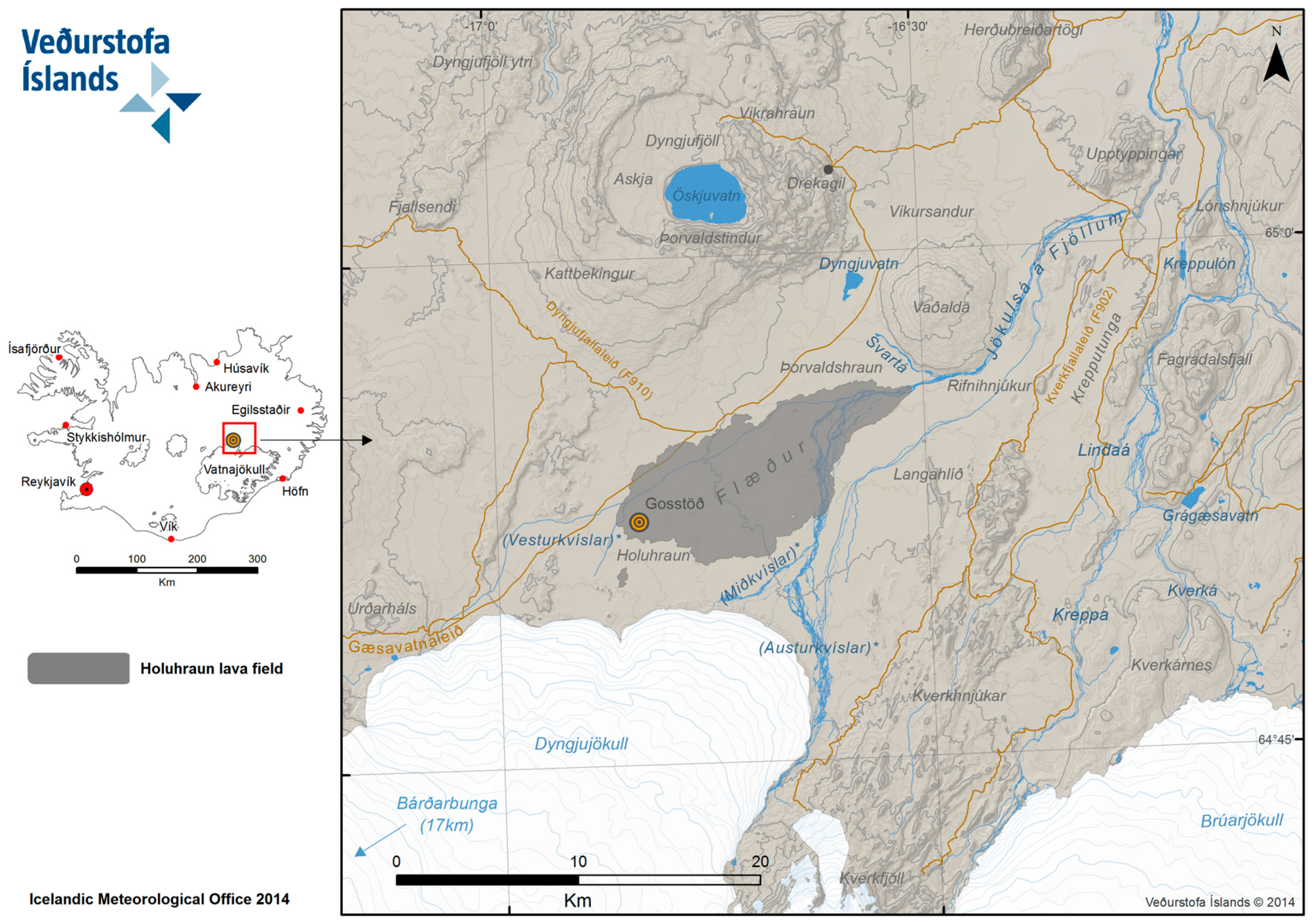
Study Area
2. Infrared Remote Sensing in Volcanoes
3. Datasets and Preprocessing
3.1. Datasets
3.2. Atmospheric and Emissivity Correction
4. Method
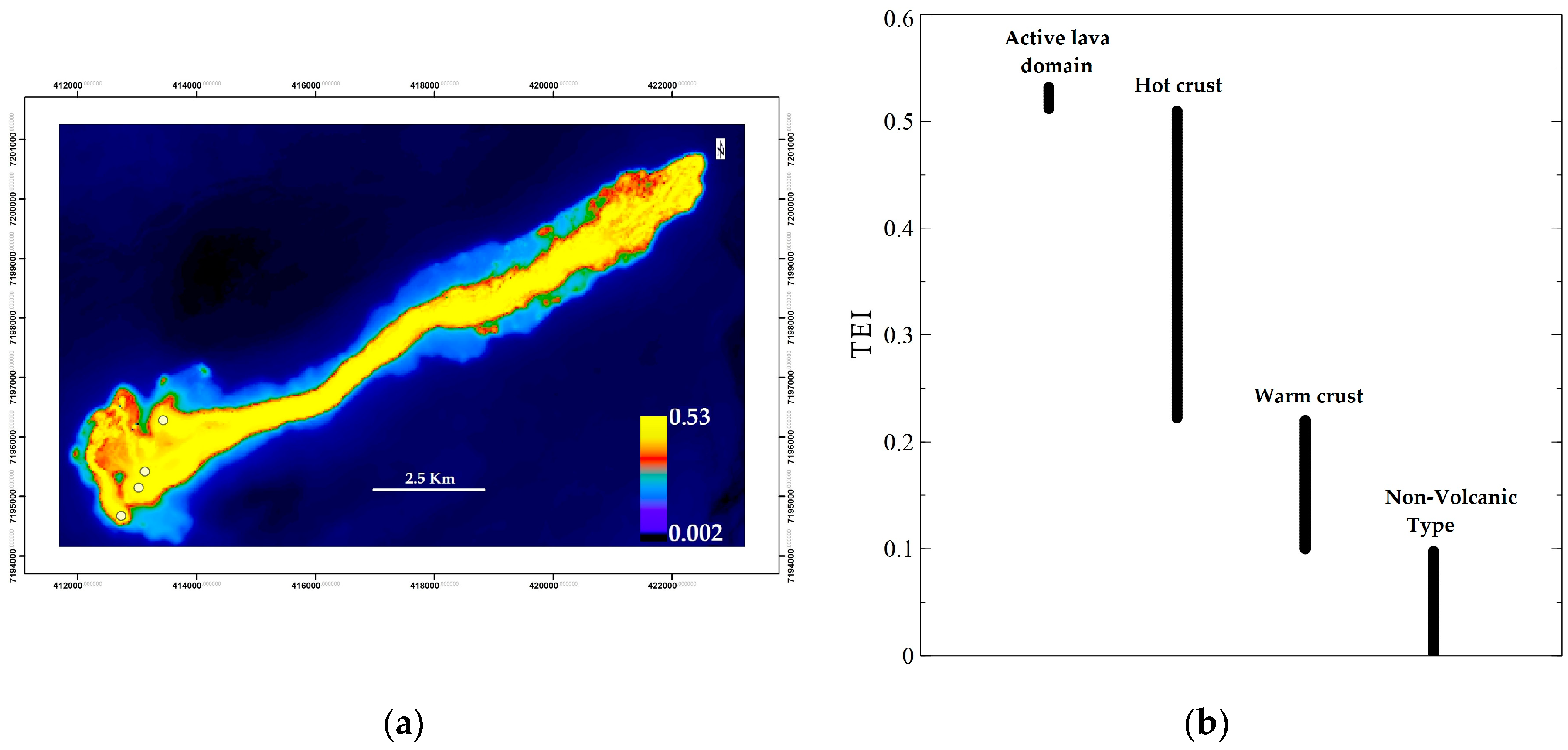
4.1. Thermal Eruption Index (TEI)
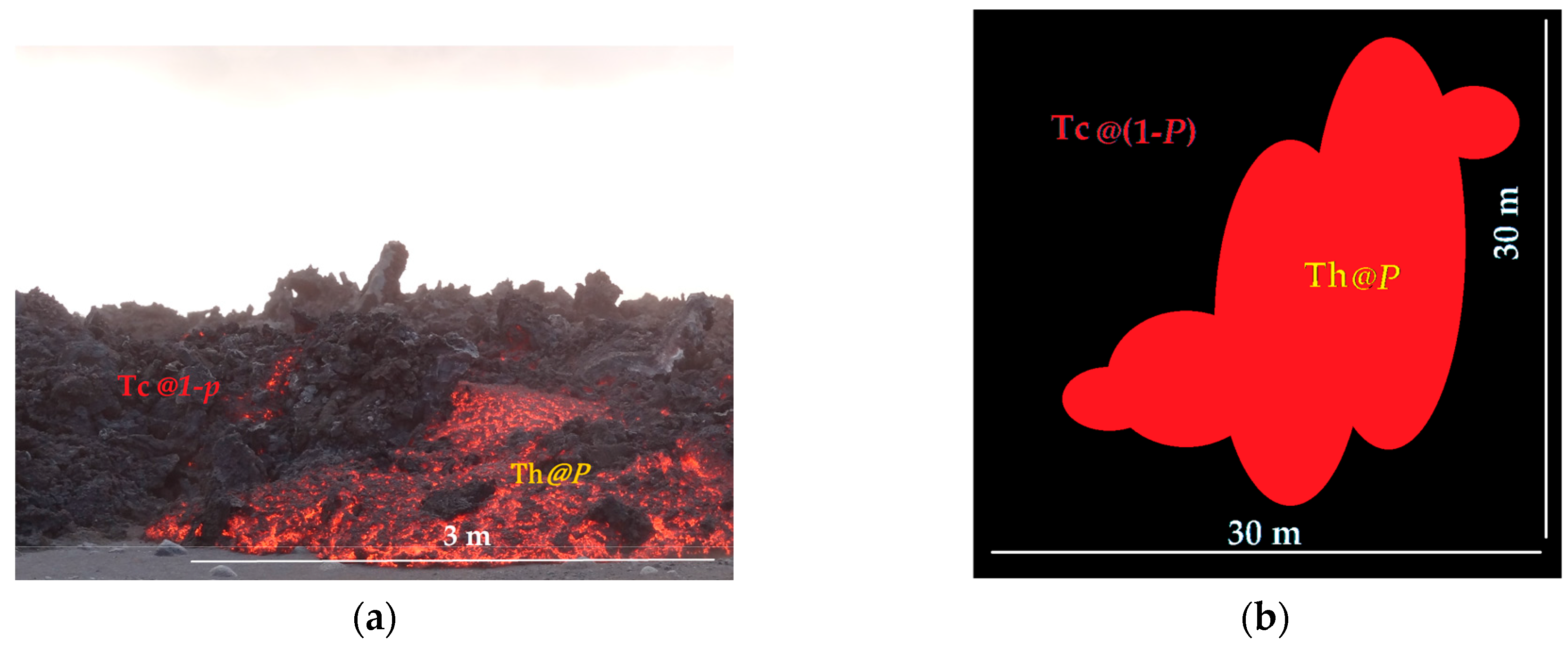
4.2. Dual-Band Method
4.3. Radiant Flux Estimation
4.4. Convective Flux Estimation
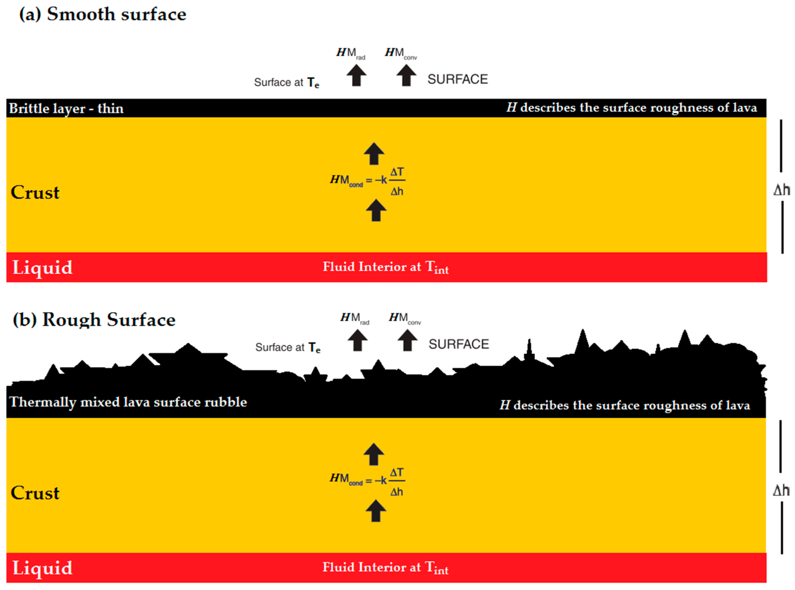
4.5. Crust Thickness Model
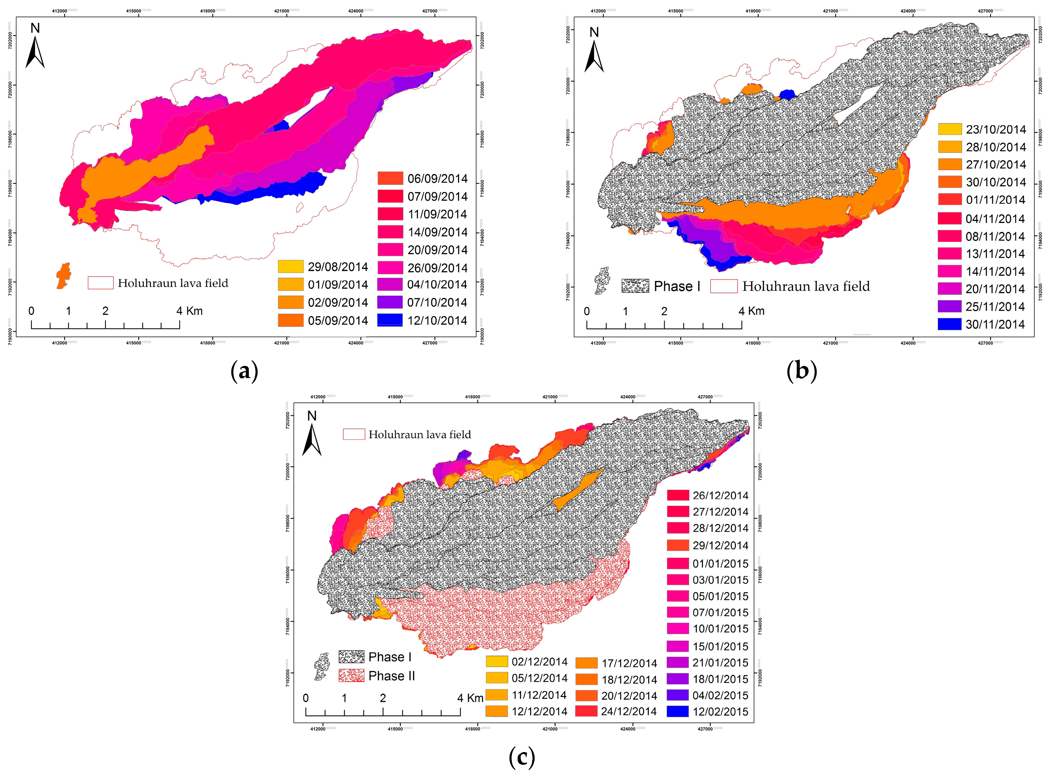
5. Results
5.1. TEI Hotspots Anomaly
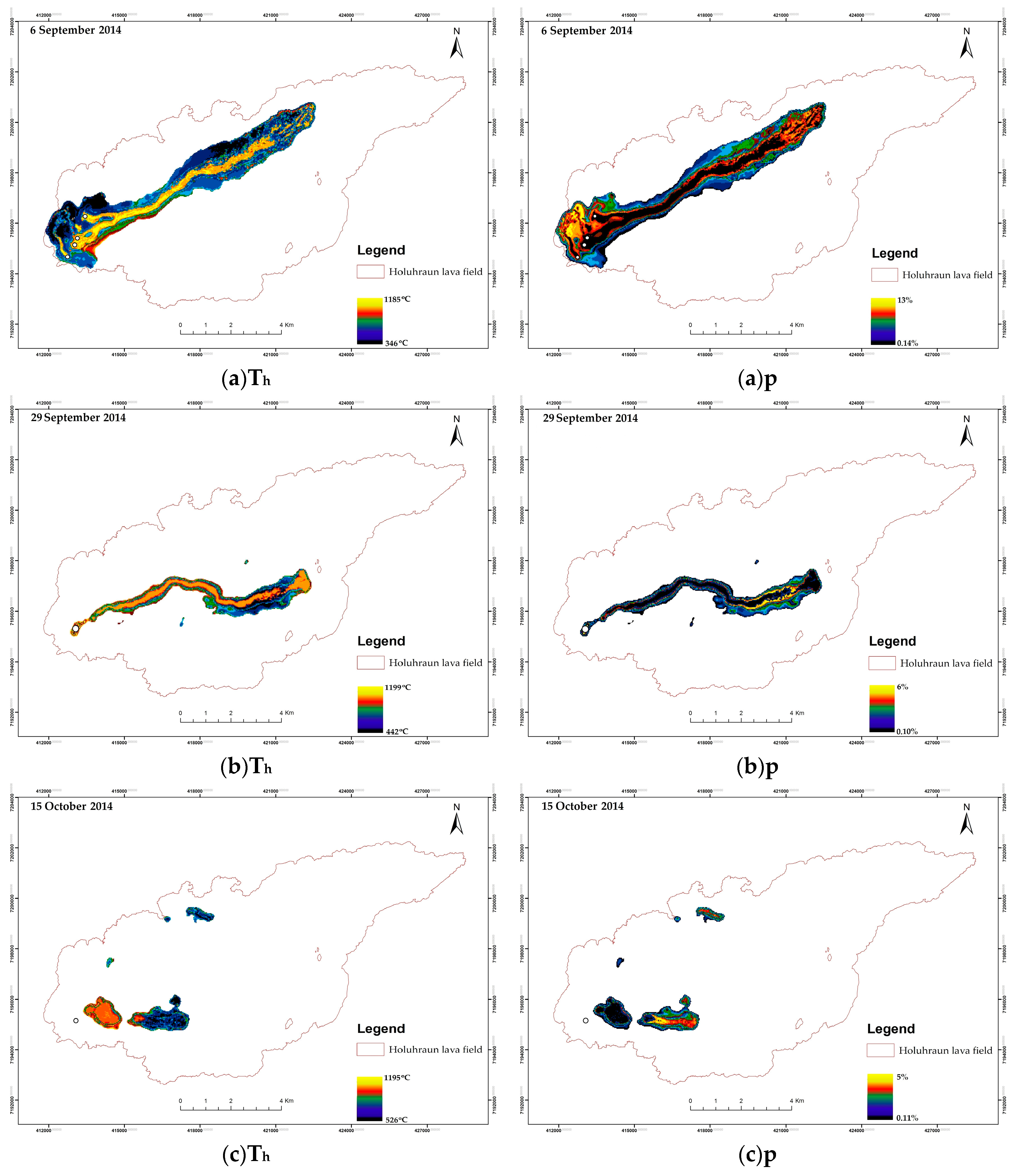
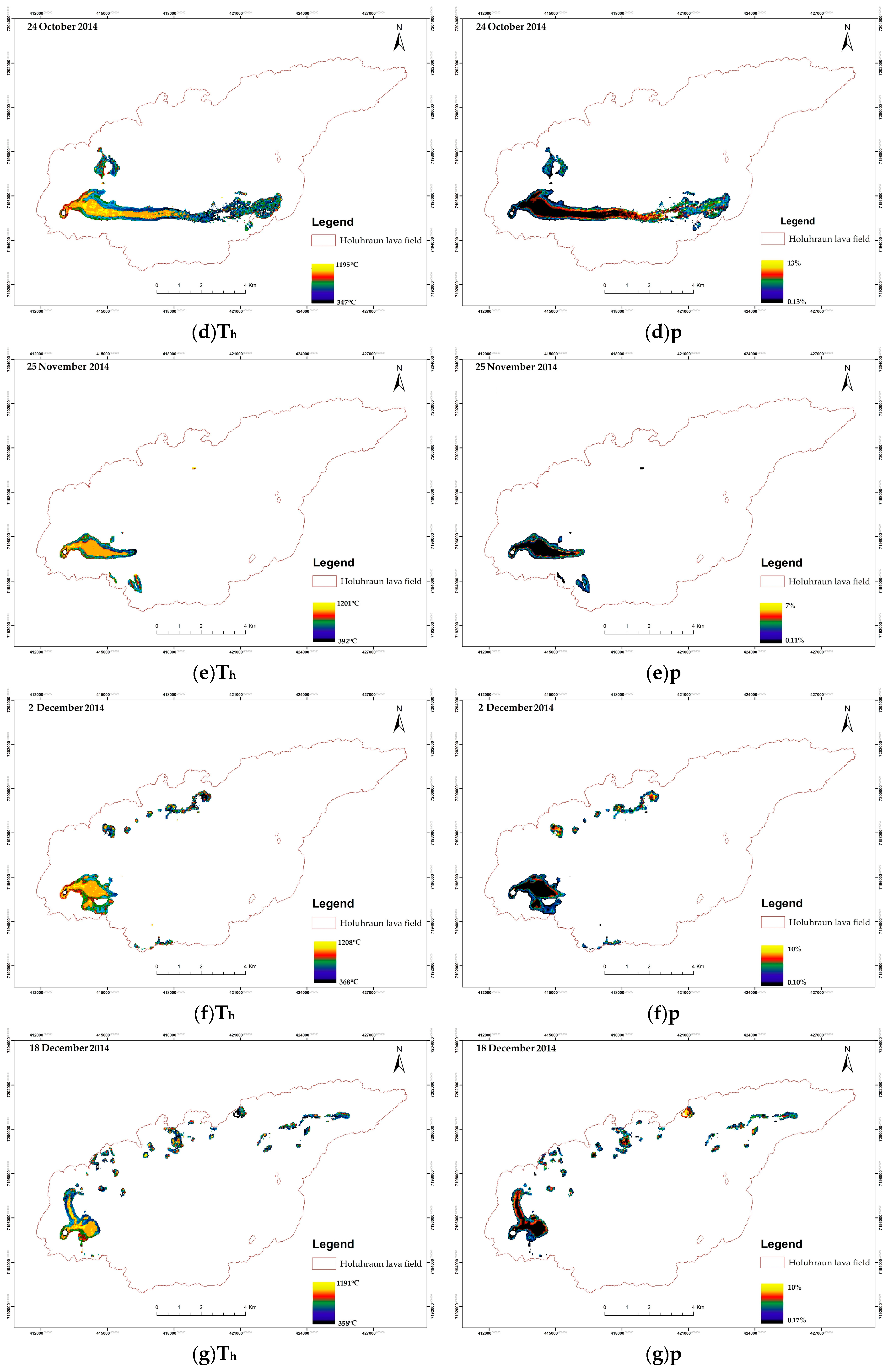
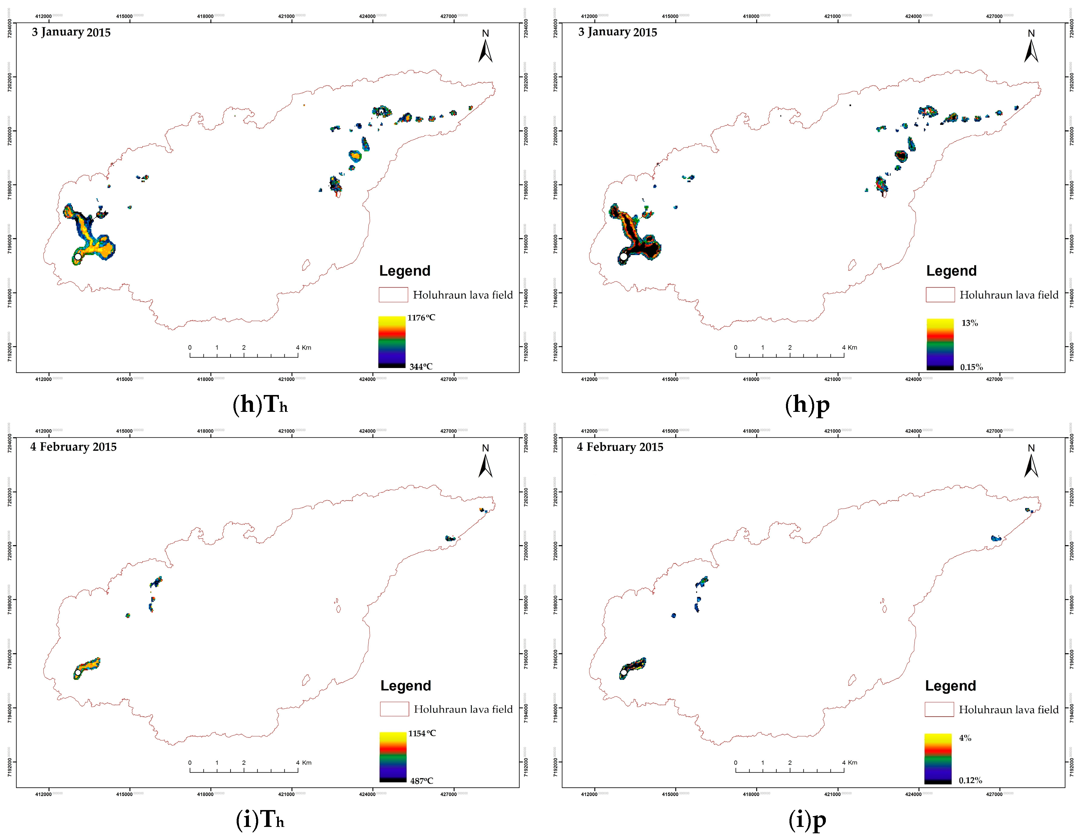
5.2. Spatial Distribution of Th and p
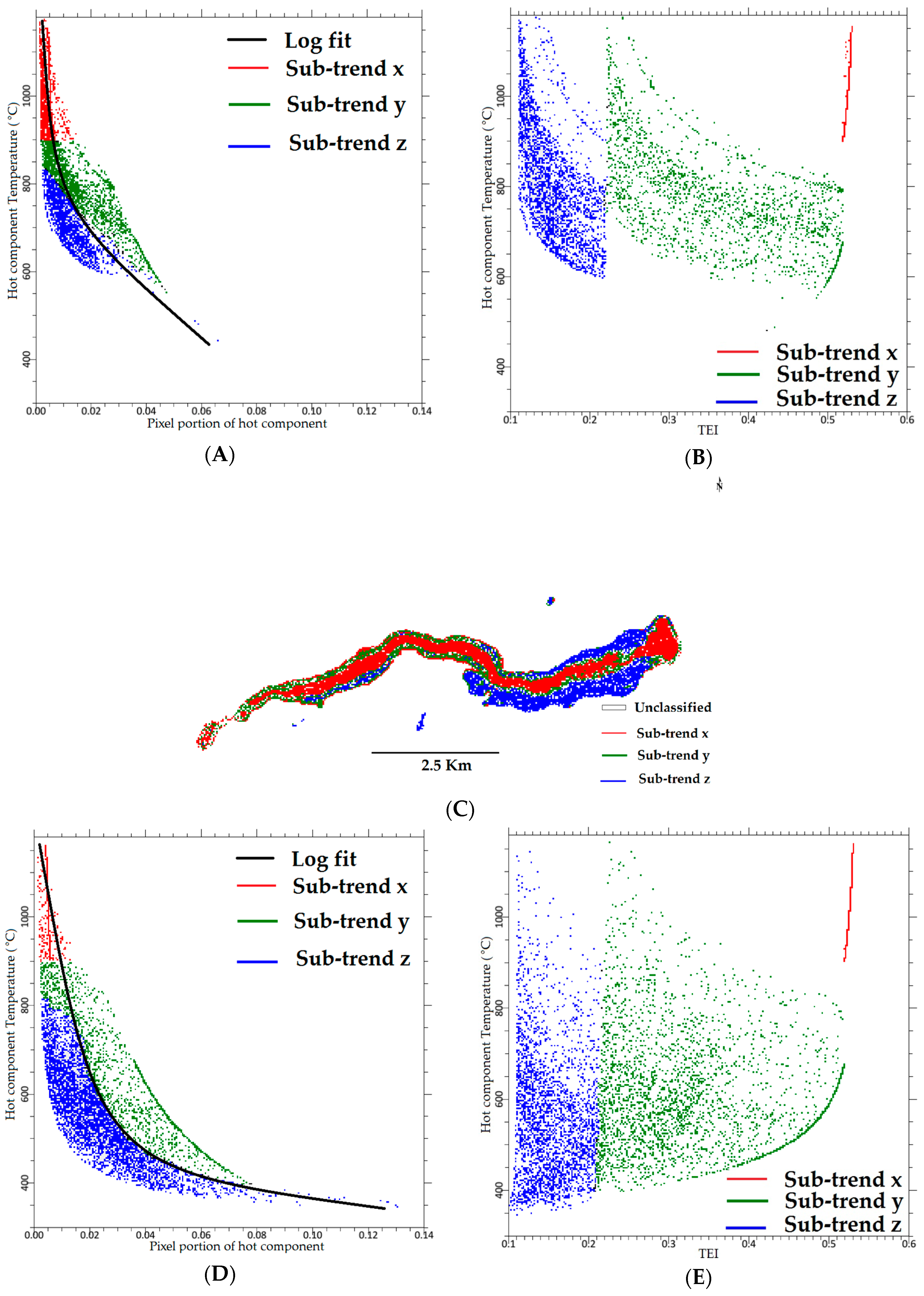
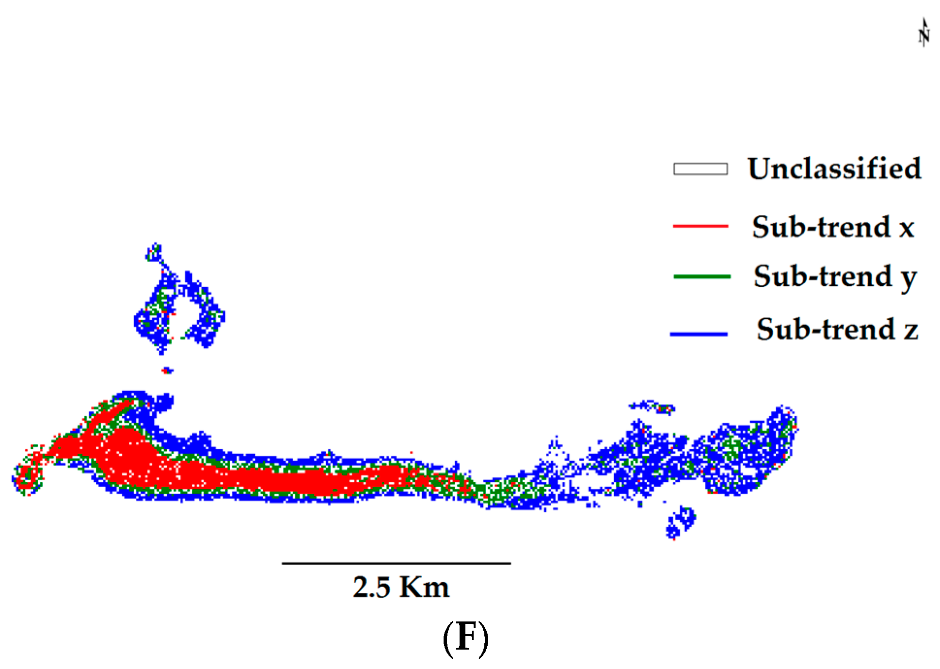
5.3. Trend Th vs. p and TEI
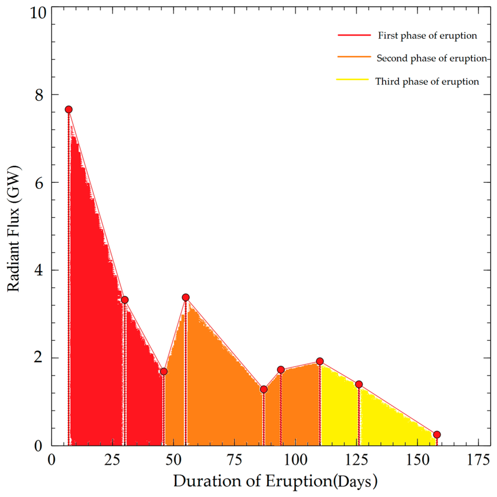
5.4. Radiant Flux Time Series during 2014–2015 Holuhraun Eruption
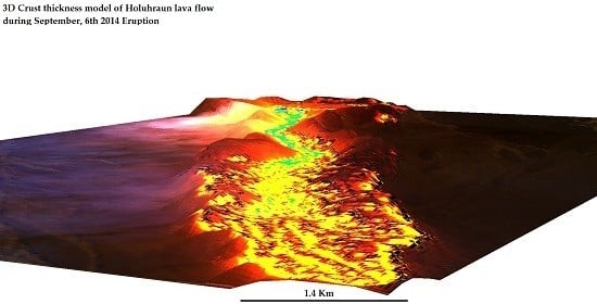
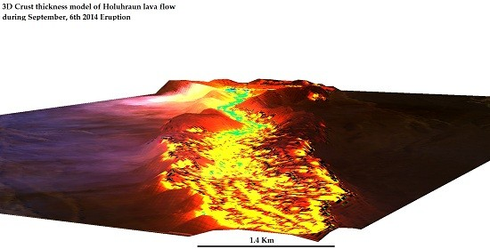
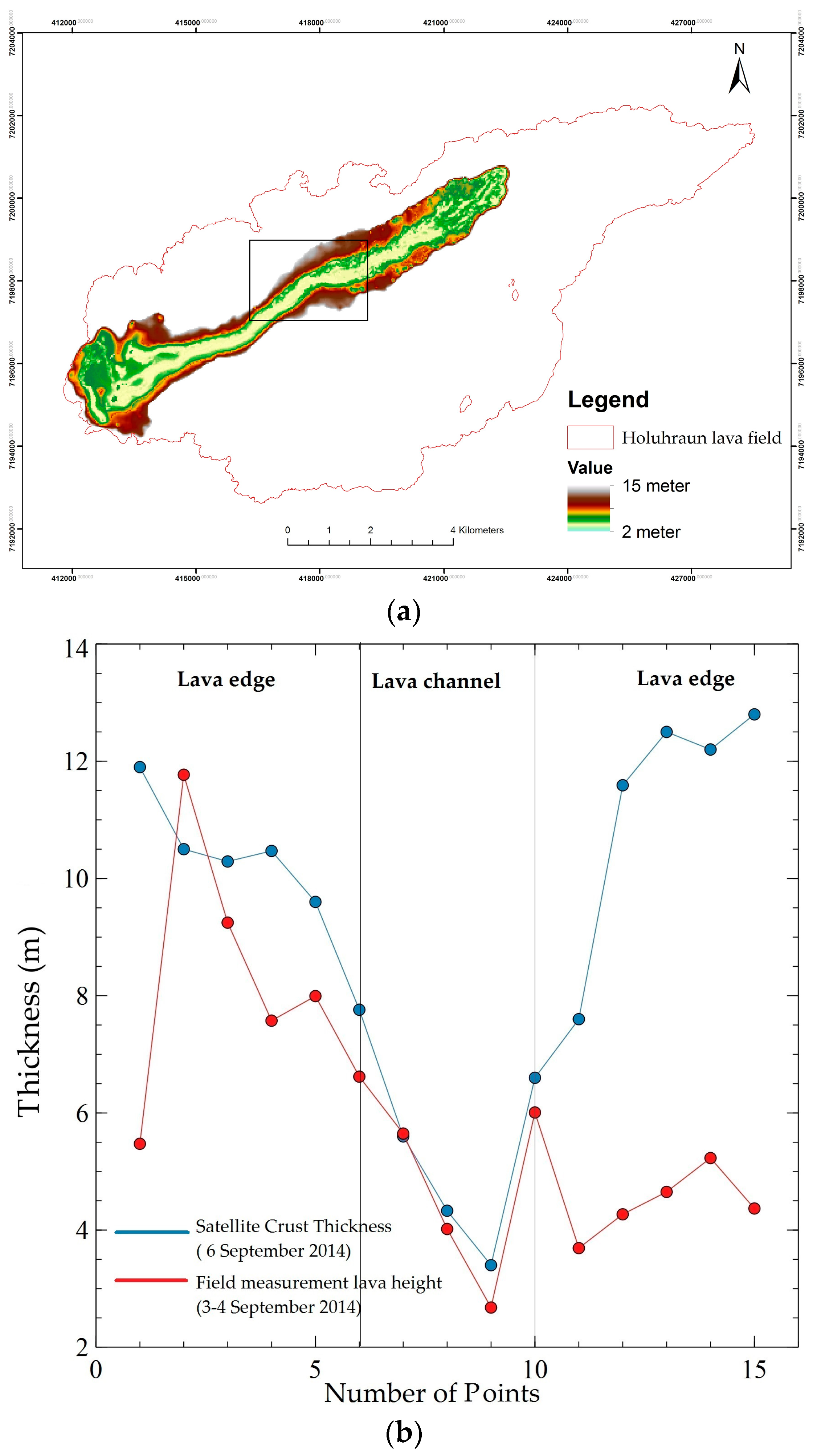
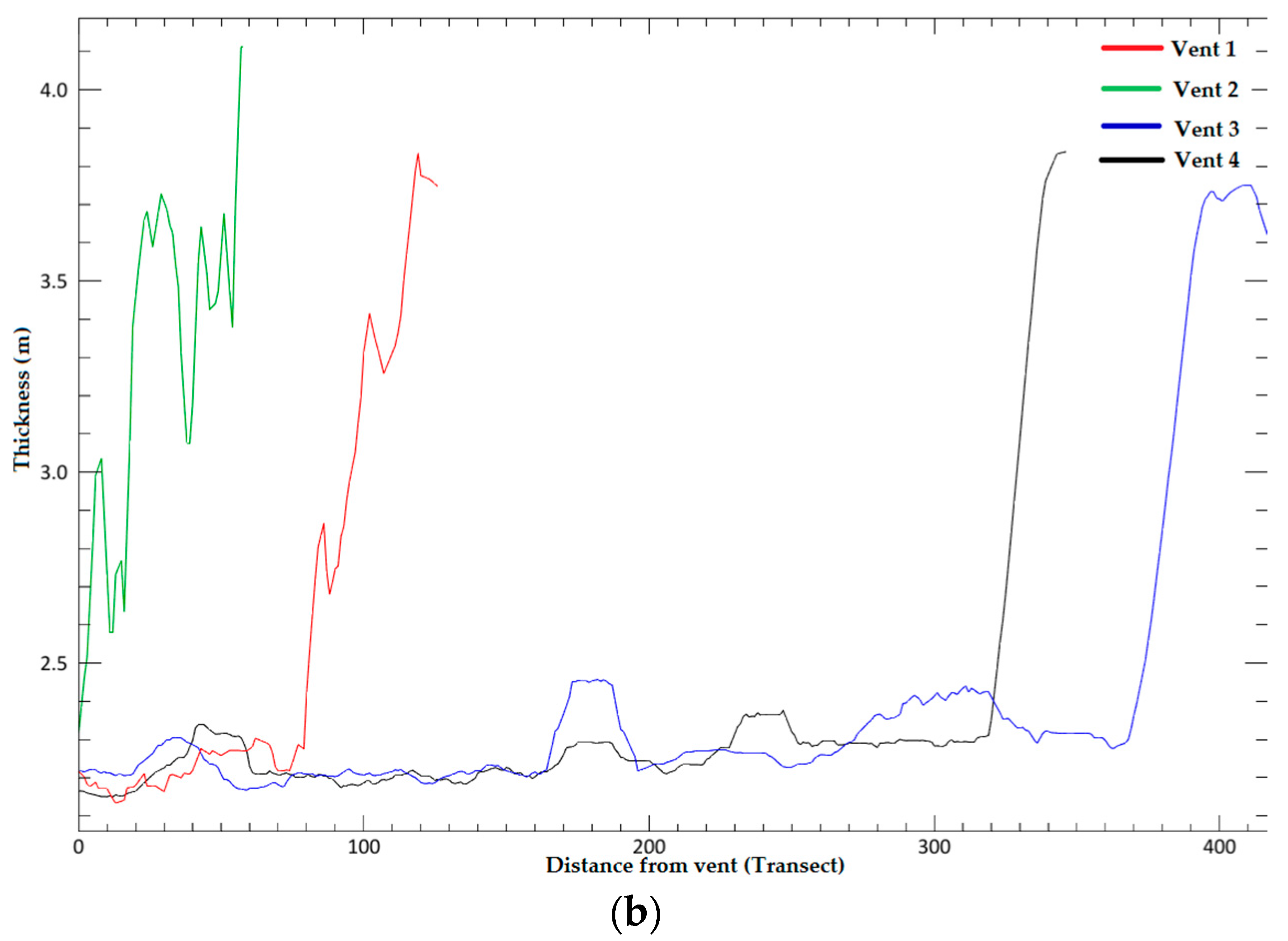
5.5. Crust Thickness Model of Lava Flow
6. Discussions
7. Conclusions
Acknowledgments
Author Contributions
Conflicts of Interest
Appendix A

Appendix B

Appendix C


Appendix D


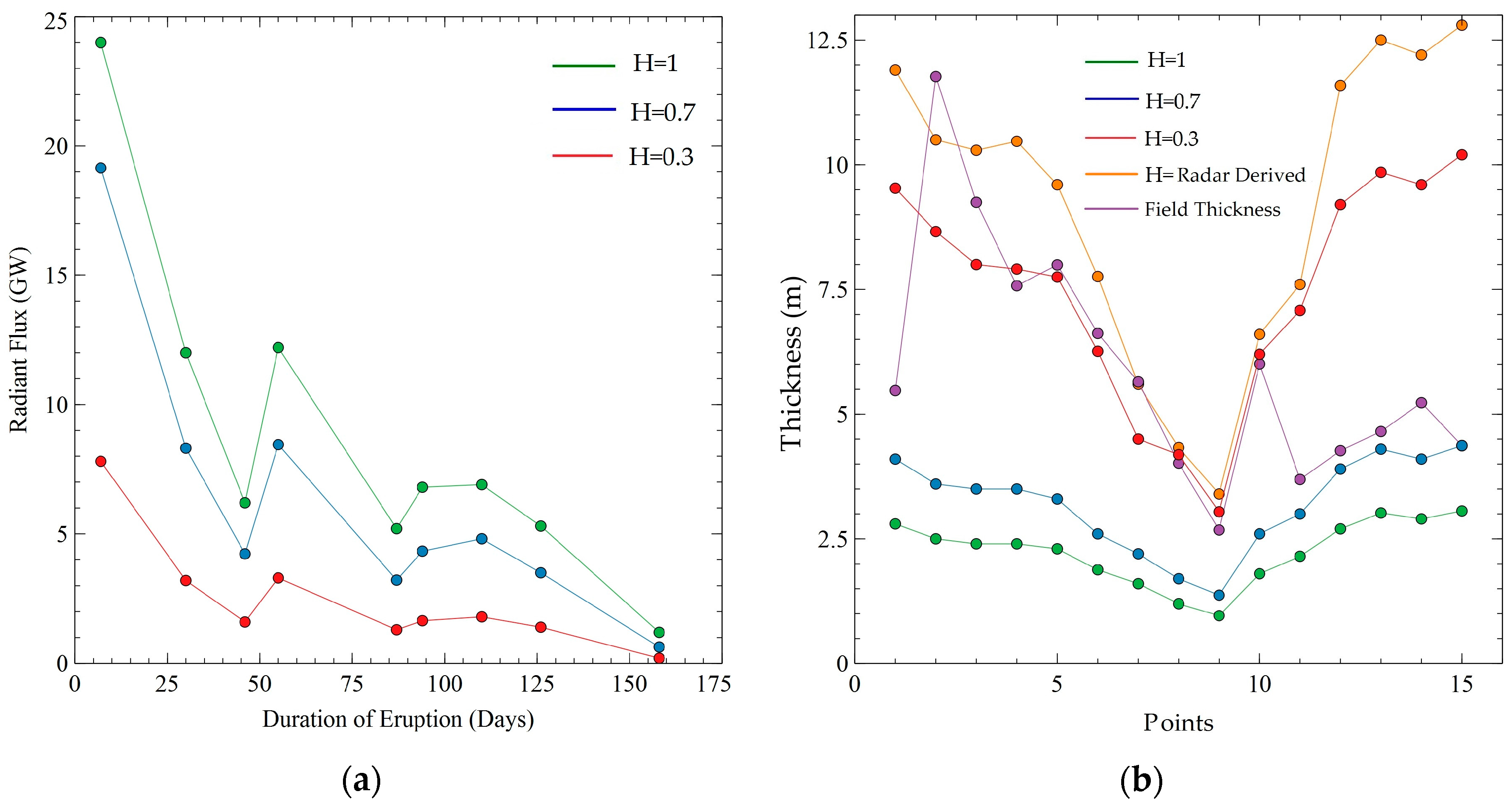
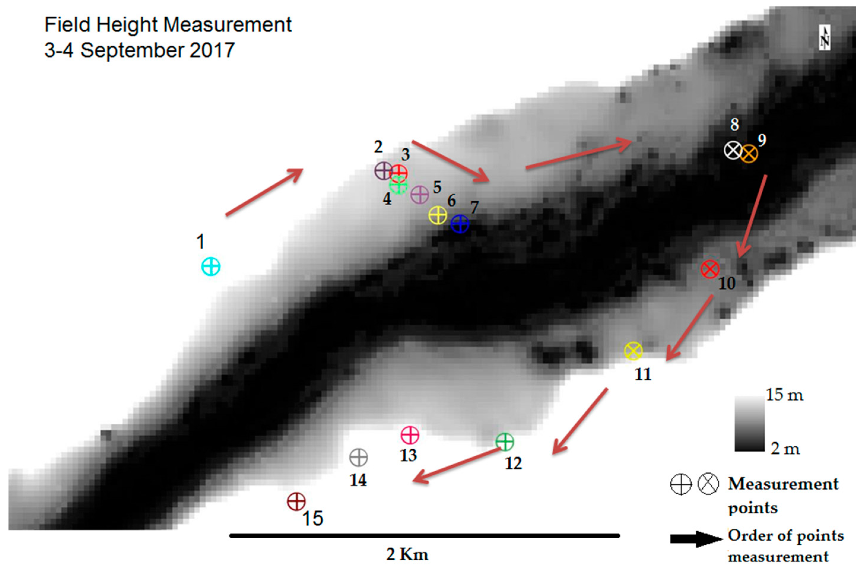
| Points | Height | Crust Thickness in 6 September 2014 from Satellite | Distance Points to Lava | Date |
|---|---|---|---|---|
| 1 | 5.47336 | 11.9 | 72 | 2014-09-03T08:39:40Z |
| 2 | 11.76946 | 10.5 | 144 | 2014-09-03T07:59:53Z |
| 3 | 9.24672 | 10.29 | 144 | 2014-09-03T07:59:53Z |
| 4 | 7.573852 | 10.47 | 84 | 2014-09-03T08:15:07Z |
| 5 | 7.993413 | 9.6 | 90 | 2014-09-03T08:20:59Z |
| 6 | 6.618929 | 7.76 | 35 | 2014-09-03T08:25:16Z |
| 7 | 5.647851 | 5.6 | 41 | 2014-09-03T08:32:52Z |
| 8 | 4.018422 | 4.33 | 21 | 2014-09-04T07:52:11Z |
| 9 | 2.676691 | 3.4 | 13.3 | 2014-09-04T07:44:08Z |
| 10 | 6.007832 | 6.6 | 34.1 | 2014-09-04T07:35:15Z |
| 11 | 3.691354 | 7.6 | 16.7 | 2014-09-04T07:27:34Z |
| 12 | 4.269408 | 11.59 | 17.4 | 2014-09-04T07:16:23Z |
| 13 | 4.651991 | 12.5 | 23.7 | 2014-09-04T07:11:51Z |
| 14 | 5.230504 | 12.2 | 24.5 | 2014-09-04T07:03:49Z |
| 15 | 4.36857 | 12.8 | 20 | 2014-09-04T06:57:22Z |
References
- Pedersen, G.B.M.; Höskuldsson, A.; Dürig, T.; Thordarson, T.; Jónsdóttir, I.; Riishuus, M.S.; Óskarsson, B.V.; Dumont, S.; Magnusson, E.; Gudmundsson, M.T.; et al. Lava field evolution and emplacement dynamics of the 2014–2015 basaltic fissure eruption at Holuhraun, Iceland. J. Volcanol. Geotherm. Res. 2017, 340, 155–169. [Google Scholar] [CrossRef]
- Pedersen, G.; Höskuldsson, A.; Riishuus, M.S.; Jónsdóttir, I.; Thórdarson, T.; Gudmundsson, M.T.; Durmont, S. Emplacement dynamics and lava field evolution of the flood basalt eruption at Holuhraun , Iceland : Observations from field and remote sensing data. In EGU General Assembly; European Geosciences Union: Vienna, Austria, 2016; Volume 18, p. 13961. [Google Scholar]
- Kolzenburg, S.; Giordano, D.; Thordarson, T.; Höskuldsson, A.; Dingwell, D.B. The rheological evolution of the 2014/2015 eruption at Holuhraun, central Iceland. Bull. Volcanol. 2017, 79, 45. [Google Scholar] [CrossRef]
- Icelandic Meteorological Office Holuhraun. Available online: http://en.vedur.is/earthquakes-and-volcanism/articles/nr/3122 (accessed on 11 May 2017).
- Thordarson, T.; Höskuldsson, Á. Postglacial volcanism in Iceland. Jökull 2008, 58, 197–228. [Google Scholar]
- Dürig, T.; Gudmundsson, M.; Högnadóttir, T.; Jónsdóttir, I. Estimation of lava flow field volumes and volumetric effusion rates from airborne radar profiling and other data: Monitoring of the Nornahraun (Holuhraun) 2014/15 eruption in Iceland. In European Geosciences Union, General Assembly; European Geosciences Union: Vienna, Austria, 2015; Volume 17, p. 8519. [Google Scholar]
- Gíslason, S.; Stefánsdóttir, G.; Pfeffer, M.A.; Barsotti, S.; Jóhannsson, T.; Galeczka, I.; Bali, E.; Sigmarsson, O.; Stefánsson, A.; Keller, N.S.; et al. Environmental pressure from the 2014–15 eruption of Bárðarbunga volcano, Iceland. Geochem. Perspect. Lett. 2015, 1, 84–93. [Google Scholar] [CrossRef]
- Wright, R.; Rothery, D.A.; Blake, S.; Harris, A.J.L.; Pieri, D.C. Simulating the response of the EOS Terra ASTER sensor to high-temperature volcanic targets. Geophys. Res. Lett. 1999, 26, 1773–1776. [Google Scholar] [CrossRef]
- Urai, M. Heat discharge estimation using satellite remote sensing data on the Iwodake volcano in Satsuma-Iwojima, Japan. Earth Planets Space 2002, 54, 211–216. [Google Scholar] [CrossRef]
- Oppenheimer, C. Lava flow cooling estimated from Landsat Thematic Mapper infrared data: The Lonquimay Eruption (Chile, 1989). J. Geophys. Res. Solid Earth 1991, 96, 21865–21878. [Google Scholar] [CrossRef]
- Harris, A.; Blake, S.; Rothery, D.A.; Stevens, N.F. A chronology of the 1991 to 1993 Mount Etna eruption using advanced very high resolution radiometer data:Implications for real-time thermal volcano monitoring. J. Geophys. Res. 1997, 102, 7985–8003. [Google Scholar] [CrossRef]
- Abrams, M.; Pieri, D.; Realmuto, V.; Wright, R. Using EO-1 hyperion data as hyspIRI preparatory data sets for volcanology applied to Mt Etna, Italy. IEEE J. Sel. Top. Appl. Earth Obs. Remote Sens. 2013, 6, 375–385. [Google Scholar] [CrossRef]
- Lombardo, V.; Buongiorno, M.F. Lava flow thermal analysis using three infrared bands of remote-sensing imagery: A study case from Mount Etna 2001 eruption. Remote Sens. Environ. 2006, 101, 141–149. [Google Scholar] [CrossRef]
- Lombardo, V.; Silvestri, M.; Spinetti, C. Near real-time routine for volcano monitoring using infrared satellite data. Ann. Geophys. 2011, 54, 522–534. [Google Scholar]
- Wright, R.; Garbeil, H.; Harris, A.J.L. Using infrared satellite data to drive a thermo-rheological/stochastic lava flow emplacement model: A method for near-real-time volcanic hazard assessment. Geophys. Res. Lett. 2008, 35, 1–5. [Google Scholar] [CrossRef]
- Lombardo, V.; Buongiorno, M.F.; Pieri, D.; Merucci, L. Differences in Landsat TM derived lava flow thermal structures during summit and flank eruption at Mount Etna. J. Volcanol. Geotherm. Res. 2004, 134, 15–34. [Google Scholar] [CrossRef]
- Wright, R.; Garbeil, H.; Davies, A.G. Cooling rate of some active lavas determined using an orbital imaging spectrometer. J. Geophys. Res. Solid Earth 2010, 115, 1–14. [Google Scholar] [CrossRef]
- Piscini, A.; Lombardo, V. Volcanic hot spot detection from optical multispectral remote sensing data using artificial neural networks. Geophys. J. Int. 2014, 196, 1525–1535. [Google Scholar] [CrossRef]
- Dozier, J. A method for satellite identification of surface temperature fields of subpixel resolution. Remote Sens. Environ. 1981, 11, 221–229. [Google Scholar] [CrossRef]
- Harris, A. Thermal Remote Sensing of Active Volcanoes: A User’s Manual; Cambridge University Press: Cambridge, UK, 2013. [Google Scholar]
- Lombardo, V.; Merucci, L.; Buongiorno, M.F. Wavelength influence in sub-pixel temperature retrieval using the dual-band technique. Ann. Geophys. 2006, 49, 227–234. [Google Scholar]
- Blackett, M. An Overview of Infrared Remote Sensing of Volcanic Activity. J. Imaging 2017, 3, 13. [Google Scholar] [CrossRef]
- Oppenheimer, C.; Rothery, D.A.; Pieri, D.C.; Abrams, M.J.; Carere, V. Analysis of Airborne Visible/Infrared Imaging Spectrometer (AVTRIS) data of volcanic hot spots. Int. J. Remote Sens. 1993, 14, 2919–2934. [Google Scholar] [CrossRef]
- Wright, R.; Flynn, L.; Garbeil, H.; Harris, A.; Pilger, E. Automated volcanic eruption detection using MODIS. Remote Sens. Environ. 2002, 82, 135–155. [Google Scholar] [CrossRef] [Green Version]
- Di Martino, G.; Iodice, A.; Riccio, D.; Ruello, G. Volcano monitoring via fractal modeling of lava flows. In Proceedings of the 2008 2nd Workshop on Use of Remote Sensing Techniques for Monitoring Volcanoes and Seismogenic Areas, USEReST 2008, Naples, Italy, 11–14 November 2008. [Google Scholar]
- Dharmawan, I.A.; Ulhag, R.Z.; Endyana, C.; Aufaristama, M. Numerical Simulation of non-Newtonian Fluid Flows through Fracture Network. IOP Conf. Ser. 2016, 29, 12030. [Google Scholar] [CrossRef]
- Pieri, D.C.; Glaze, L.S.; Abrams, M.J. Thermal radiance observations of an active lava flow during the June 1984 eruption of Mount Etna. Geology 1990, 18, 1018–1022. [Google Scholar] [CrossRef]
- Ferrucci, F.; Hirn, B. Automated monitoring of high-temperature volcanic features: From high-spatial to very-high-temporal resolution. Geol. Soc. Lond. Spec. Publ. 2016, 426, 159–179. [Google Scholar] [CrossRef]
- Martinez, O.S.; Cruz, D.M.; Chavarin, J.U.; Bustos, E.S. Rough Surfaces Profiles and Speckle Patterns Analysis by Hurst Exponent Method. J. Mater. Sci. Eng. 2014, 3, 759–766. [Google Scholar]
- Shepard, M.K.; Campbell, B.A.; Bulmer, M.H.; Farr, T.G.; Gaddis, L.R.; Plaut, J.J. The roughness of natural terrain: A planetary and remote sensing perspective. J. Geophys. Res. Planets 2001, 106, 32777–32795. [Google Scholar] [CrossRef]
- Reynolds, H.I.; Gudmundsson, M.T.; Högnadóttir, T.; Magnússon, E.; Pálsson, F. Subglacial volcanic activity above a lateral dyke path during the 2014–2015 Bárdarbunga-Holuhraun rifting episode, Iceland. Bull. Volcanol. 2017, 79, 38. [Google Scholar] [CrossRef]
- Rothery, D.A.; Francis, P.W.; Wood, C.A. Volcano monitoring using short wavelength infrared data from satellites. J. Geophys. Res. 1988, 93, 7993–8008. [Google Scholar] [CrossRef]
- Wright, R.; Blackett, M.; Hill-Butler, C. Some observations regarding the thermal flux from Earth’s erupting volcanoes for the period of 2000 to 2014. Geophys. Res. Lett. 2015, 42, 282–289. [Google Scholar] [CrossRef]
- Rossi, C.; Minet, C.; Fritz, T.; Eineder, M.; Bamler, R. Temporal monitoring of subglacial volcanoes with TanDEM-X—Application to the 2014-2015 eruption within the Bárdarbunga volcanic system, Iceland. Remote Sens. Environ. 2016, 181, 186–197. [Google Scholar] [CrossRef]


| Product ID | Date |
|---|---|
| LC82170152014249LGN00 | 6 September 2014 |
| LC82180142014272LGN00 | 29 September 2014 |
| LC82180142014288LGN00 | 15 October 2014 |
| LC80642292014297LGN00 | 24 October 2014 |
| LC80642302014329LGN00 | 25 November 2014 |
| LC80652292014336LGN00 | 2 December 2014 |
| LC80652292014352LGN00 | 18 December 2014 |
| LC80652292015003LGN00 | 3 January 2015 |
| LC82180142015035LGN00 | 4 February 2015 |
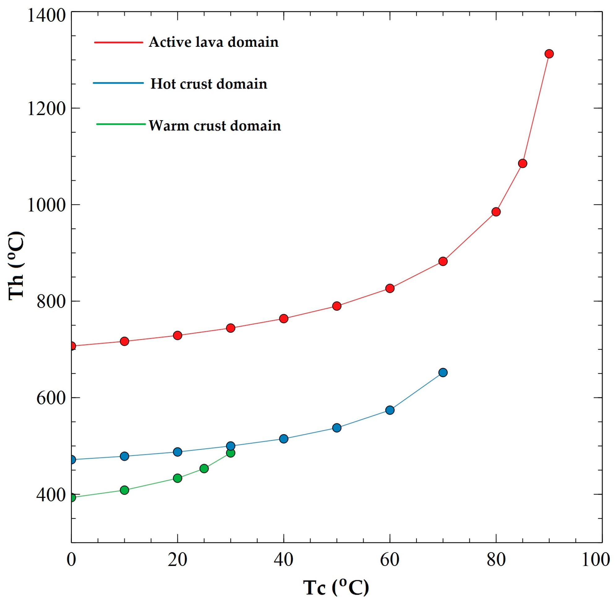
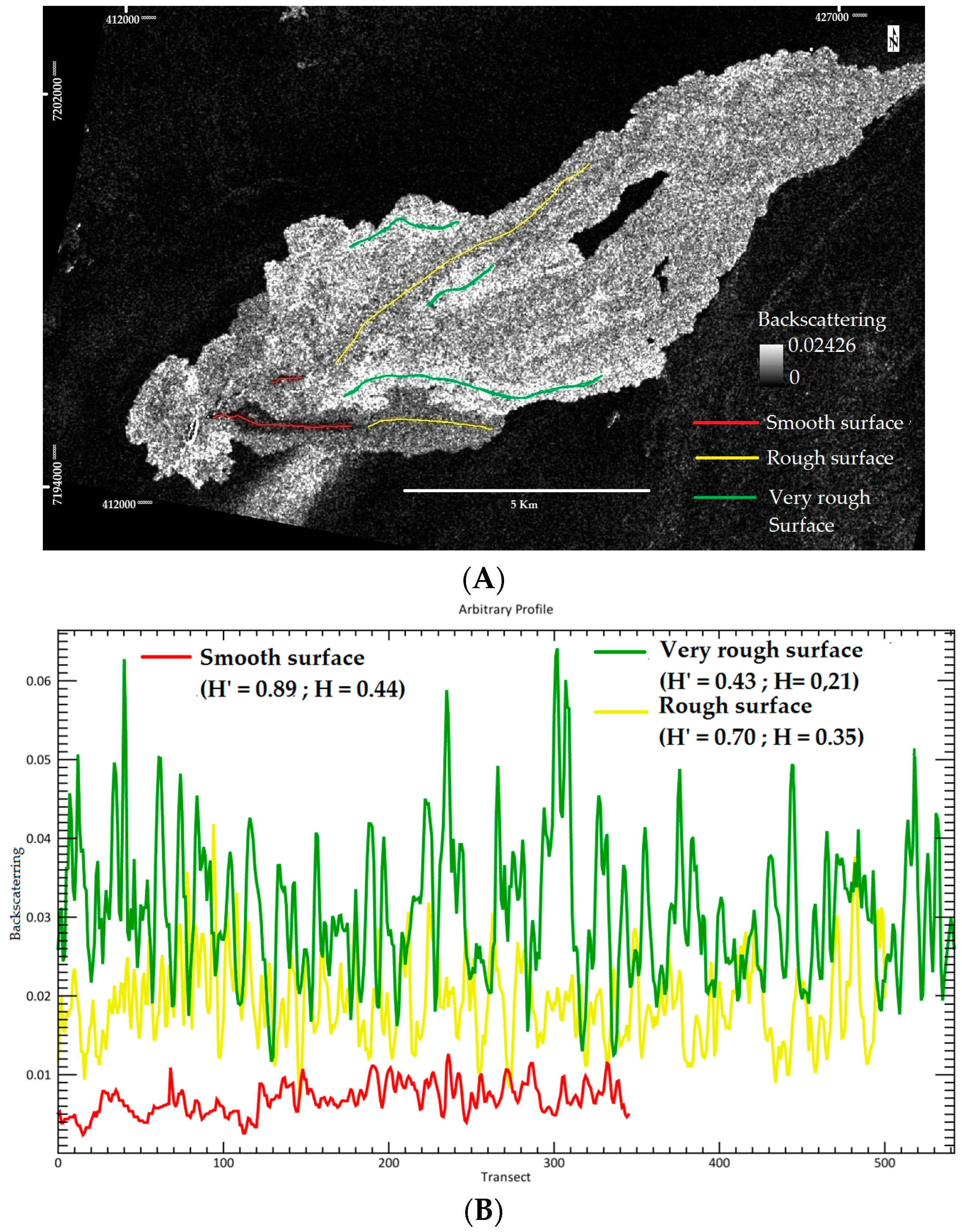
| H’ | H (after Normalized) | Description | Thermal Domain |
|---|---|---|---|
| 0.43 | 0.21 | Very rough surface (Aa flow, large, tilted, spinny pates [30]). | Warm crust |
| 0.70 | 0.35 | Rough surface (Aa flow, small spinny plates [30]). | Hot crust |
| 0.89 | 0.44 | Smooth surface (Sheet pahoehoe flow, channel, roppy structure [30]). | Active lava |
| Date | Th min (°C) | Th max (°C) | Th average (°C) | p Min | p Max | p Average | TEI Min | TEI Max |
|---|---|---|---|---|---|---|---|---|
| 6 September 2014 | 346 | 1185 | 685 | 0.14% | 13% | 2.2% | 0.102 | 0.53 |
| 29 September 2014 | 442 | 1199 | 885 | 0.10% | 6% | 1% | 0.100 | 0.53 |
| 15 October 2014 | 526 | 1195 | 816 | 0.11% | 5% | 1.2% | 0.101 | 0.53 |
| 24 October 2014 | 347 | 1195 | 705 | 0.13% | 13% | 2% | 0.100 | 0.53 |
| 25 November 2014 | 392 | 1201 | 901 | 0.11% | 7% | 0.08% | 0.102 | 0.53 |
| 2 December 2014 | 368 | 1208 | 770 | 0.10% | 10% | 1.4% | 0.101 | 0.53 |
| 18 December 2014 | 358 | 1191 | 677 | 0.17% | 10% | 2.1% | 0.100 | 0.53 |
| 3 January 2015 | 344 | 1176 | 689 | 0.15% | 13% | 2% | 0.102 | 0.53 |
| 4 February 2015 | 487 | 1154 | 790 | 0.12% | 4% | 1% | 0.101 | 0.53 |
© 2018 by the authors. Licensee MDPI, Basel, Switzerland. This article is an open access article distributed under the terms and conditions of the Creative Commons Attribution (CC BY) license (http://creativecommons.org/licenses/by/4.0/).
Share and Cite
Aufaristama, M.; Hoskuldsson, A.; Jonsdottir, I.; Ulfarsson, M.O.; Thordarson, T. New Insights for Detecting and Deriving Thermal Properties of Lava Flow Using Infrared Satellite during 2014–2015 Effusive Eruption at Holuhraun, Iceland. Remote Sens. 2018, 10, 151. https://0-doi-org.brum.beds.ac.uk/10.3390/rs10010151
Aufaristama M, Hoskuldsson A, Jonsdottir I, Ulfarsson MO, Thordarson T. New Insights for Detecting and Deriving Thermal Properties of Lava Flow Using Infrared Satellite during 2014–2015 Effusive Eruption at Holuhraun, Iceland. Remote Sensing. 2018; 10(1):151. https://0-doi-org.brum.beds.ac.uk/10.3390/rs10010151
Chicago/Turabian StyleAufaristama, Muhammad, Armann Hoskuldsson, Ingibjorg Jonsdottir, Magnus Orn Ulfarsson, and Thorvaldur Thordarson. 2018. "New Insights for Detecting and Deriving Thermal Properties of Lava Flow Using Infrared Satellite during 2014–2015 Effusive Eruption at Holuhraun, Iceland" Remote Sensing 10, no. 1: 151. https://0-doi-org.brum.beds.ac.uk/10.3390/rs10010151