Onboard Spectral and Spatial Cloud Detection for Hyperspectral Remote Sensing Images

1
School of Automation Science and Electrical Engineering, Beihang University, No.37 Xueyuan Road, Beijing 100191, China
2
China Academy of Space Technology (CAST), Beijing 100094, China
3
China Centre for Resources Satellite Data and Application, No.5 Fengxian East Road, Beijing 100094, China
4
School of Mathematics and Systems Science, Beihang University, No.37 Xueyuan Road, Beijing 100191, China
*
Author to whom correspondence should be addressed.
Remote Sens. 2018, 10(1), 152; https://0-doi-org.brum.beds.ac.uk/10.3390/rs10010152
Submission received: 15 November 2017
/
Revised: 15 January 2018
/
Accepted: 16 January 2018
/
Published: 20 January 2018
(This article belongs to the Section Remote Sensing Image Processing)
Abstract
:The accurate onboard detection of clouds in hyperspectral images before lossless compression is beneficial. However, conventional onboard cloud detection methods are not applicable all the time, especially for shadowed clouds or darkened snow-covered surfaces that are not identified in normalized difference snow index (NDSI) tests. In this paper, we propose a new spectral-spatial classification strategy to enhance the performance of an orbiting cloud screen obtained on hyperspectral images by integrating a threshold exponential spectral angle map (TESAM), adaptive Markov random field (aMRF) and dynamic stochastic resonance (DSR). TESAM is applied to roughly classify cloud pixels based on spectral information. Then aMRF is used to do optimal process by using spatial information, which improved the classification performance significantly. Nevertheless, misclassifications occur due to noisy data in the onboard environments, and DSR is employed to eliminate noise data produced by aMRF in binary labeled images. We used level 0.5 data from Hyperion as a dataset, and the average tested accuracy of the proposed algorithm was 96.28% by test. This method can provide cloud mask for the on-going EO-1 and related satellites with the same spectral settings without manual intervention. Experiments indicate that the proposed method has better performance than the conventional onboard cloud detection methods or current state-of-the-art hyperspectral classification methods.
1. Introduction
As hyperspectral remote sensing technologies progress, hyperspectral imaging techniques [1] are being widely used in many fields such as meteorology, earth observations and military affairs. Meteorological satellites have obvious advantages in monitoring the continuity, spatiality and tendency of qualitative changes in the atmospheric environment, providing indispensable information for the omnidirectional monitoring of global atmosphere state. Unlike meteorological satellites, earth observation satellites primarily sense changes in earth surfaces due to city planning, geological prospecting, military reconnaissance and natural disasters. Regardless of the application background, most remote sensing images contain clouds that, especially in the visible and infrared range, strongly affect the received electromagnetic radiation. Historically, clouds cover approximately 70% of the earth’s surface [2] and play a dominant role in the energy and water cycles of our planet. However, the earth’s radiative budget or aerosol detection as influenced by clouds is not the focus of this paper. Typically, a piece of hyperspectral image data contains over 200 spectral bands, presenting challenges for both data transmission and storage [3]. Future earth exploration missions will face unprecedented data volumes generated, due to improvements in detector, optics and onboard data processing technologies. Compared with meteorological satellites, the data sizes of earth observation satellites are larger due to their higher spatial resolutions and revisiting frequencies. Satellite and ground links (download speed) are heavily utilized, and readers can refer to the Appendix A for details. It is given the fact that almost all these sensors have only limited memory capacity and the data transmission from satellites to ground become inevitable for further data analysis [4]. Additionally, the large data volumes affect mission requirements for the entire data processing chain, including onboard digitization, storage, downlink, ground processing and distribution [5]. These bottlenecks will curtail the instrument duty cycles, reducing science and application yield [6]. Based on the specific applications, clouds are catalysts for meteorological research [7,8,9], yet are impediments for earth observation [10,11]. For meteorological researchers, image data should be fully retained and transmitted to the ground for further research. For non-meteorological researchers, clouds, as a disturbance factor for earth explorations, will shaded the surface features of the target region. As invalid data, data of over cloud regions can be discarded onboard directly. Therefore, removing or retaining clouds constitutes two kinds of onboard processing strategy.
Data compression is necessary for onboard processing, but lossy compression methods are unsuitable for hyperspectral images used in cases demanding accuracy, because the images are intended to be analyzed automatically using computers [12]. Bandwidth constraints have motivated new advanced lossless compression techniques such as the KLT algorithm [13,14,15], which has achieved compression rates of four or greater. Efforts to optimize lossless methods eventually face theoretical limits, but data size continues to increase, propelling research on other techniques that can further reduce data volumes while preserving scientific gains. It is likely that only a part of an entire image carries information of interest in a specific case. At this time, rather than the entire image, only the region of interest (ROI) needs to be compressed [16]. In this way, higher compression ratios can be achieved by simply not compressing those invalid data regions. Cloud regions are regarded to be arbitrarily shaped, and ROI maps encoded using the ARLE [17] algorithm will be applied to describe the shapes of cloud regions. An ROI map with pixel of 400 × 256 can maximally be compressed into 3200 bits, achieving a compression ratio of 1:256, 0.002% of the original data size (fairly small). Excising the cloud region data before compression could significantly reduce data sizes, yet an accurate algorithm for real-time cloud detection in instrument hardware remains absent.
Most onboard cloud detection methods are based on the radiometric features of clouds. “Classical” cloud detection applies threshold tests to image spectral properties [18,19]. Pixels whose values fall outside of valid ranges are marked as clouds. For example, the algorithms corresponding to MODIS compare the selected visible and near-infrared (VNIR) and near-infrared (NIR) bands to predetermined thresholds and then aggregate the results in different combinations depending on land type [20,21,22,23]. These algorithms use a combination of 14 wavelengths and more than 40 tests. This underscores the intrinsic difficulty of constructing a universal and complete cloud screening procedure. We focus on the visible short wave infrared (VSWIR) electromagnetic spectrum from 0.4–2.5 μm. There are many studies of cloud detection at those wavelengths, and algorithms vary in their assumptions and complexity. Of direct relevance to this work, onboard cloud detection has been demonstrated onboard the EO-1 spacecraft [24]. EO-1 cloud detection uses the solar zenith angle to compute the apparent top-of-atmosphere (TOA) reflectance. It then applies a branching sequence of threshold tests based on carefully crafted spectral ratios to distinguish clouds and bright landforms such as snow, ice, and desert sand. EO-1 cloud detection also acts as a data filtering step prior to onboard cryosphere and flood classification [25,26]. To our knowledge, it is the only previous case of cloud screening performed on orbit. Another kind of onboard cloud detection algorithms is mainly based on ACCA. They are used to give cloud-cover (CC) predictions to reduce cloud contamination in acquired scenes [27,28,29]. These onboard cloud detection methods are based on threshold decision trees (TDT) in general.
Even more complex algorithms on the ground side have been proposed. Some state of-the-art cloud-screening techniques estimate optical path from absorption features such as the oxygen A band, as in Gómez-Chova et al. [30] or Taylor et al [31]. Thermal infrared (TIR) channels can add brightness temperature information. Minnis et al., predicted clear-sky brightness temperature values using ambient temperature and humidity and then excised pixels outside those intervals [32]. Texture cues can be utilized to recognize clouds by their high spatial heterogeneity [33]. Martins et al., demonstrated that a simple spatial analysis, i.e., the standard deviation of VNIR isotropic reflectances in a 3 × 3 pixel window, reliably discriminated clouds from aerosol plumes over ocean scenes [34]. Jin hu Bian et al., proposed a spectral signature and spatiotemporal context method to distinguish snow from clouds [35]. A Markov random field model was developed to segment hyperspectral image. Murtagh et al., represented spatial dependency using a prior probabilistic Markov random field [36]. Haoyang Yu et al., proposed an adaptive MRF method combined with SVM and achieved a good terrains classification performance [37]. Probabilistic models are another kind of cloud detection method. Gómez-Chova et al., used a Gaussian mixture model to produce posterior probabilities. The Bayesian probabilistic model of Merchant et al. combines observational data with prior predictions from atmospheric forecasts, leading to true probabilistic predictions [38]. David R. proposed the decision theoretic method (DTM) based on a Bayesian probabilistic model. The DTM achieved negligible false positives in cloud screening [39]. Recently, deep learning has been widely used in classifications of HSI. Li Wei et al., proposed hyperspectral image classification using deep pixel-pair features [1]. Bin Pan et al., proposed a kind of vertex component analysis network that achieved better performance than some state-of-the-art methods [40].
TDT methods have more commission errors that are at high altitudes or at low solar illumination where snow is misclassified as clouds. The probabilistic model methods and learning-based methods (such as neural networks or supervised learning) have more omission errors. The omission errors are associated with optically thin clouds over underlying surfaces because of the incompleteness of training samples for this kind of cloud. Focusing on these problems, our method uses an exponential spectral angle map, Markov random field and dynamic stochastic resonance. The rest of this paper is organized as follows. Section 2 introduces the problems of onboard cloud detection methods in detail. The proposed methodology for cloud detection is introduced in Section 3. Performance evaluations for different operation scenarios using a decade-year historical image archive of the “classic” Hyperion spectrometer is provided in Section 4. Section 5 discusses the advantages, limitations and applicability of the proposed method. Section 6 presents the conclusions.
2. Related Work
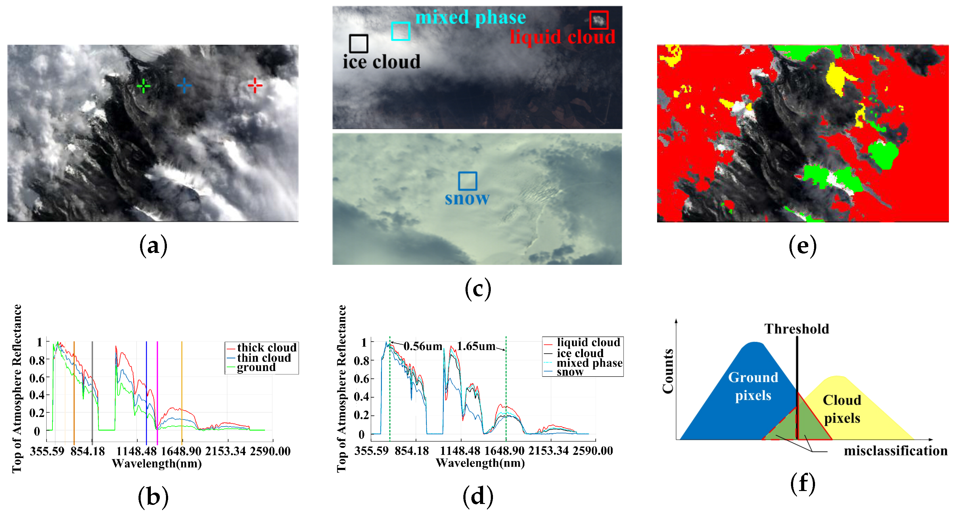
TDT methods are typically used for onboard cloud detection now. Table 1 shows the typically used bands of several TDT methods, all of which include normalized difference snow index (NDSI). NDSI tests have difficulties detecting shadowed cloud and darkened snow covered surfaces [41], as well thin clouds. A detected scene is shown in Figure 1. As presented in Figure 1a,e, it is hard to completely classify the cloud pixels merely in spectral feature space due to various complex factors. As the optical thicknesses of clouds differs, some omission errors (the yellow region in Figure 1e of cloud detection occurred. The three spectral curves in Figure 1b were sampled from the three crosses marked in (a). The spectral differences between thin and thick clouds are distinct, especially in NIR bands. The reflectances of the thin cloud were respectively 62.2% and 14.8% of those of the thick clouds were in the vicinity of 1.25 μm and 1.65 μm, respectively, because the spectrum of thin clouds was heavily affected by the underlying surface. The large reflectance deviation entailed a failure to achieve complete cloud detection for one set of parameters. Except for omission errors, commission errors also exist in cloud detection (the green part in Figure 1e), because the spectral features of clouds and snow-covered surfaces are sometimes similar under NDSI (differing particles and illumination generate different reflectances). Figure 1c represents two scenes containing liquid clouds, mixed phase clouds, ice clouds and snow. The spectral normalization of the four materials are shown in Figure 1d, in which the black curve represents the TOA reflectance of a piece of a thick ice cloud, the cyan curve represents the TOA reflectance of an unknown portion of a mixed phase cloud, where the ice phase may be dominant, the red curve represents the TOA reflectance of a piece of a liquid cloud, and the blue curve represents the reflectance of snow. The normalized spectra of the three cloud types of cloud are highly consistent. The greatest differences among three curves appear near 1.65 μm. Specifically, liquid clouds share the highest reflectance near 1.65 μm, whereas the reflectance of mixed phase clouds is lower and that of ice clouds is the lowest. Figure 1d indicates that the spectral envelope of snow differs from that of clouds near 1.03 μm and 1.38 μm, yet snow and clouds share almost all the same spectrum near 0.56 μm and 1.65 μm. Unfortunately, the spectrum at 1.65 μm occurred to be used by NDSI (see the boldfaced characters in Table 1). For the above two problems of the cloud detection, Figure 1f symbolically illustrates that cloud pixels and ground pixels cannot be separated completely under a TDT classifier because of the overlap of spectral features.
The influence of clouds on solar radiation is due to the reflectance, absorption and scattering of radiation by cloud particles. It depends strongly on the dimensions, altitude, opacity, thickness and composition of the clouds. The World Meteorological Organization (WMO) classifies clouds by altitude and divides the troposphere vertically into three levels; low, middle, and high. Low-level clouds are primarily constituted by water due to evaporation of water. Ice crystals constitute high-level cloud because temperature is low high altitude. Middle-level clouds are composited by water particles and ice particles. There are different types of clouds with different dimensions, opacities and other properties that depend on several parameters and result in different effects on solar radiation. Clouds are divided into ten types as seen in Table 2 . Ice crystals and water drops have different impacts on the absorption and scattering of solar radiation especially in SWIR. According to statistics from 184 scenes of Hyperion level 0.5 data, the solar reflectances of the 10 cloud types and different ground types can be seen in the electromagnetic spectrum from 0.4–2.5 μm, as shown in Figure 2. Different clouds may have different amplitudes of reflectance. After normalization, the envelopes of the spectral curves are roughly the same, as shown in Figure 2a. However, different surface features have different spectral reflectance, as shown in Figure 2b. In this paper, we paimarily focus on how to detect cloud pixels rather than recognizing different types of clouds.
The pure threshold method is a simple, efficient, and practical approach for cloud detection, but it is sensitive to background and cloud conditions, which makes it impractical for general use [42]. Compared with the threshold method, spectral angle maps (SAM) have better cloud detection performance because they take advantage of more spectral information. In this paper, we demonstrate a cloud detection algorithm that mainly uses a threshold exponential spectral angle map (TESAM), adaptive Markov random field (aMRF) and dynamic stochastic resonance (DSR). To obtain an accurate cloud cover region, we present the TESAM-aMRF-DSR method for cloud detection. The following sections describe the algorithm’s theoretical method.
3. Proposed Method
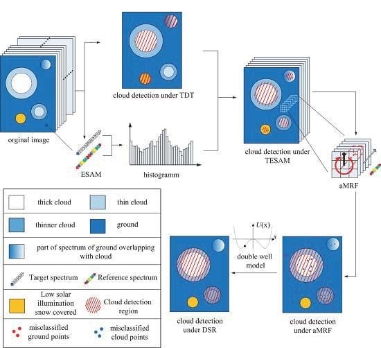
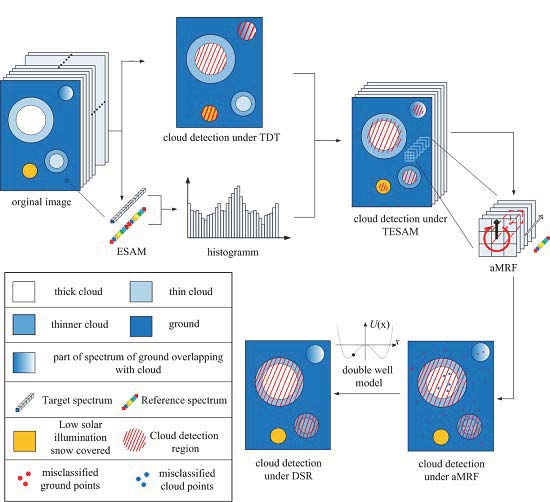
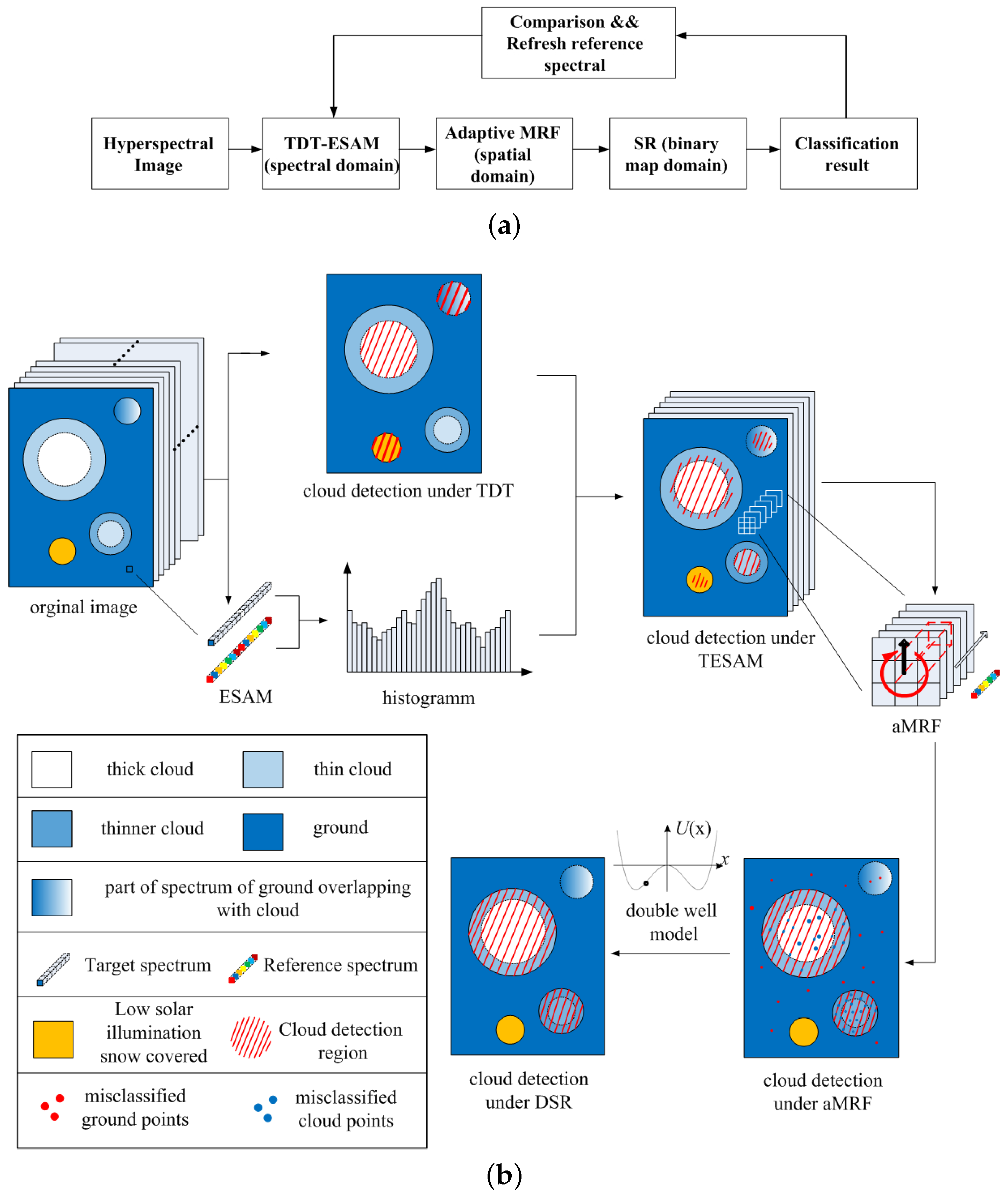
A new method is proposed to address the above-mentioned problems. The general framework of the proposed methods is shown in Figure 3a. The hyperspectral images are processed by TESAM. Initially, hyperspectral images were proposed by TESAM, which provided the basic classification result, and aMRF was then used based on the classification. The output of aMRF was then used as the input of DSR. Finally, the reference spectrum was refreshed in accordance with the final classification. The flow of the above process is as follows. TESAM is composed of TDT and ESAM. Uncertainties in illumination angle and thermodynamic phase will entail misclassifications when using TDT methods. As shown in Figure 3b, certain part of the snow-covered ground and the ground whose spectrum overlapped with the cloud spectrum were misclassified as cloud under TDT. Nevertheless, the TDT method could still be used to obtain the preliminary area of the cloud region, ESAM was instrumental in calculating the distance between two spectral vectors because it was robust to illumination variations. Representing the composition of the spectral reflectance in the form of vector. ESAM calculates the cosines of the angles between the target spectrum and the reference spectrum. The histogram was then obtained from the calculated cosines of the angles. From the acquired preliminary cloud area and histogram, we can identify whether the pixel is a cloud pixel. A distinctive feature of cloudy pixel is that the non-absorbing 0.44 μm–0.96 μm wavelengths were sensitive to cloud optical thickness (COT), and most absorbing channels within 1.03 μm–2.4 μm were sensitive to cloud effective particle radius (CER). Having taken advantage of these bands, TESAM produced little misclassification. The aMRF described the interaction between adjacent pixels by employing energy index, which is jointly determined by spectral dimension and spatial dimension. The relations among eight adjacent pixels in the spatial dimension were taken into consideration. The aMRF chose 1.38 μm–1.39 μm and 1.46 μm–1.55 μm, which primarily took advantage of vapour reflectance bands. Although the spectra of some thin cloud pixels and dark cloud pixels deviated from the threshold range, the aMRF classification results bore a small error range. The omission and commission errors were both reduced upon iterative processing using minimum energy. The aMRF was primarily applied for optimization. However, the onboard processing data were level-0.5, indicating that radiometric calibration of images was absent. Therefore, as shown in the lower right part of Figure 3b, some points whose energies had been mutated were be misclassified during the aMRF process. These misclassified points were regarded as noisy points in the binary cloud mask. DSR eliminated those noisy points by using a double-well model. By integrating attributes of adjacent pixels, DSR transferred isolated noisy points from one state to another, acting as a refinement tool.
3.1. T-ESAM
SAM calculates the angle (x,y), where x and y are N-dimensional spectral, , and , respectively:
where is the scalar product between x and y
and represents the Euclidean norm, i.e., . x represents the target spectral vector, and y represents the referenced spectral vector.
TDT methods for onboard cloud detection such as the ACCA algorithm [27] for multispectral and HCC algorithm [24] for hyperspectral and appear to be good discriminators for most cases. The performances of these cloud detection algorithms are not good enough (75% of the ACCA scores were within 10% of the actual cloud cover content) [27]. This situation can be improved under SAM. In addidtion, we encapsulated the SAM metric inside an exponential function to produce the ESAM function, which is a positive semi-definite function. The ESAM function is defined as
where k is the gain parameter. The resolution of ESAM decreases with decreasing k. Generally, k is set to 0.5 (between 0 and 1). ESAM amplifies the angular distance between two vectors.
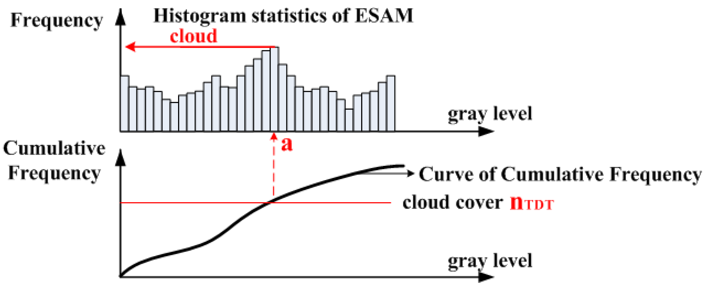
After the 3-D original hyperspectral image processing using ESAM, we can obtain a 2-D computing result. The lowest value indicates the most similar spectrum. These data are probably a cloud region if there are clouds in the image. Simultaneously, threshold algorithms also have been used to detect cloud region results. We then can obtain the classifier by combining ESAM with TDT, as shown in Figure 4. Employing the TDT method, we can obtain the number of cloud pixels n which is the solid red line. The cumulative frequency curve can be drawn when the histogram of an image has been calculated. The intersection between n and the cumulative frequency curve locates the threshold value “a” of the ESAM histogram.
The observed spectrum of instrument data forms a vector x with multiple spectral channels per pixel. The cloud-screen decision maps those pixel brightness values to a binary classification c = f(x) : →, where c represents that there is a cloud present and c represents the event that clear sky is observed. Classifier f(x) coarsely detects the cloud.
The pseudocode for the TDT algorithm combined with the ESAM algorithm, abbreviated as TDT assisted ESAM, is shown in Algorithm A1 which is in Appendix B.
3.2. aMRF Model
The MRF model provides an accurate feature representation of pixels and their neighbourhoods. The basic principle of aMRF is to integrate spatial correlation information into the posterior probability of the spectral features. Based on the maximum posterior probability principle, the classic MRF model can be expressed as follows:
where and are the mean vector and covariance matrix of class k, respectively. The neighborhood and class of pixel i are represented by and , respectively. Equation (6) separates the pixels of a remote sensing image into 2 classes: ground pixels and cloud pixels. The parameter is the weight coefficient, which is used to control the influence of the spatial term.
To obtain the local spatial weight coefficients , Chien-I Chang [43] among others used the noise-adjusted principal components (NAPC) transform. It can be uesd to obtain the first principal component to calculate the :
where represents the class-decision variance of the neighbourhood of pixel i as determined by majority voting rules and is the local variance of pixel i [44]. When is high, it can be concluded that pixel i is located in a homogeneous region. By contrast, pixel i is on a boundary when is low. The local spatial weight coefficient when = ; usually, = 1.
According to Equation (7), the aMRF model can be divided into two components: the energy of spectral term (k) and the energy of spatial term (k). Thus, Equation (7) can be represented in the form
where is the Kronecker delta function, which is defined as
The pseudocode for the TESAM algorithm combined with the aMRF algorithm, abbreviated TESAM-aMRF, is shown in Algorithm A2 which is in Appendix C.
3.3. Dynamic Stochastic Resonance (DSR) Model
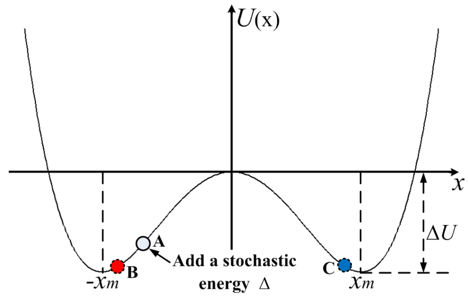
The DSR model here is used to denoise the cloud mask. In analogy to Benzi’s double-well model, the binary image pixel value is treated as the position of a particle in a double well. The addition of stochastic energy affects its transition to the strong signal state, just as a particle makes a transition from one well to another. Such a change in the state of a pixel under noise can be modelled by the Brownian motion of a particle placed in a double-well potential system, such as that shown in Figure 5. Particle A is located in the left well. The state of particle A may or may not turn over in the double well after providing stochastic energy to A. The location of particle A may be at point B if it does not turn over or at point C if it turns over. The left and the right wells represent the black and white pixels of a binary cloud mask, respectively.
A classic 1-D nonlinear dynamic system that exhibits SR is modelled with the help of the Langevin equation of motion is given below
This equation describes the motion of a particle of mass m moving in the presence of friction, . The restoring force is expressed as the gradient of a bistable potential function U(x). In addition, there is an additive stochastic force of intensity D.
If the system is heavily damped, the inertial term can be neglected. Rescaling the system in (11) with the damping term gives the stochastic overdamped Duffing equation, which is frequently used to model non-equilibrium critical phenomena as given in (12)
where U(x) is a bistable quartic potential given by
Here, a and b are positive bistable double-well parameters. The double-well system is stable at separated by a barrier of height and when is zero. The Langevin equation describes the motion of particle in a general double-well.
The pseudocode for the aMRF algorithm combined with the DSR algorithm, abbreviated as aMRF-DSR, is shown in Algorithm A3 which is in Appendix D.
4. Feasibility Study
4.1. Dataset
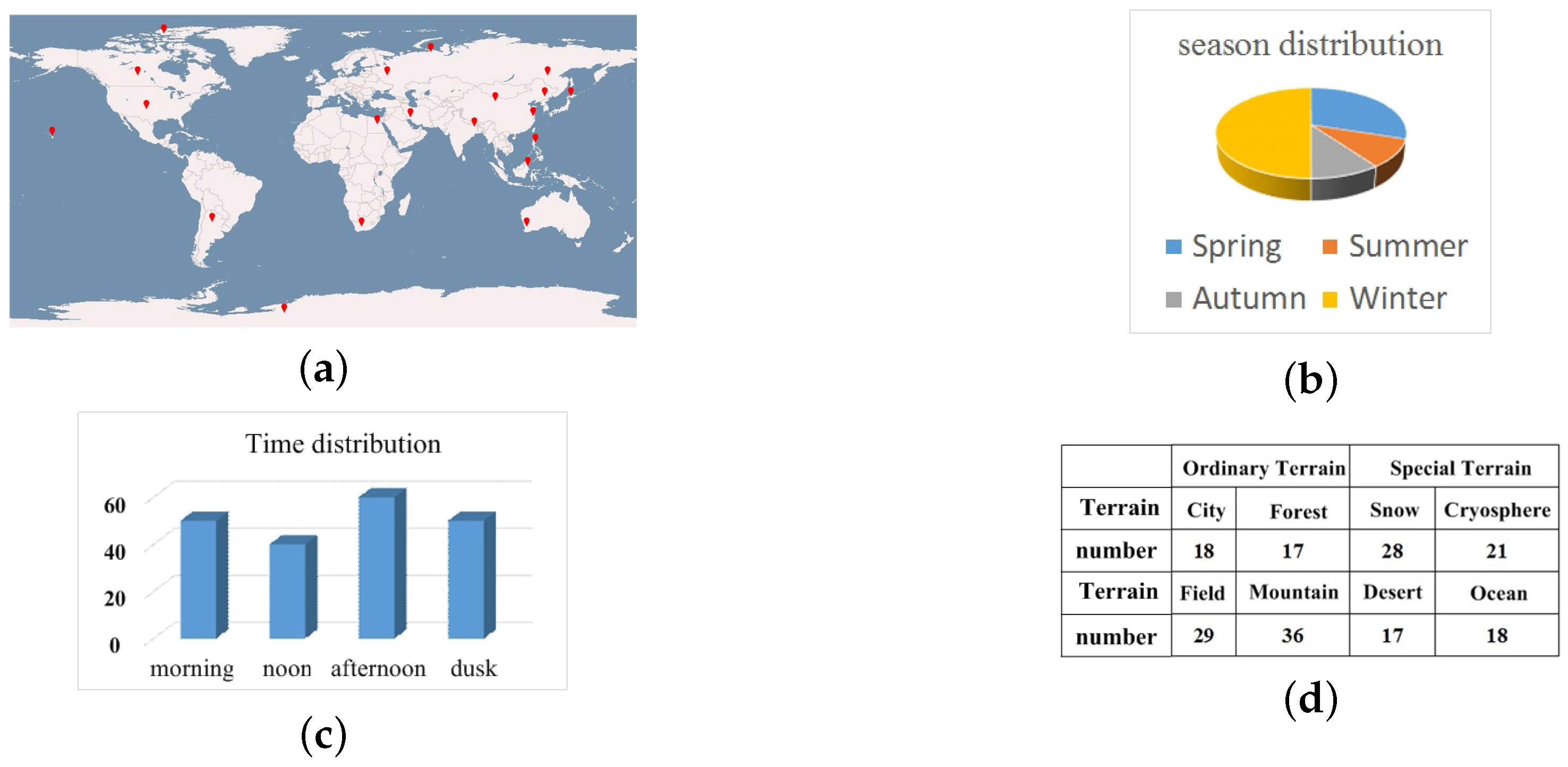
In this section, we evaluate the performance of the proposed algorithms by employing the widely used hyperspectral data from the Hyperion EO-1 sensor. The data used in onboard processing are level 0.5 and were downloaded from the USGS website. The dataset contains city, ocean, forest, mountain range, desert, snow and cryosphere terrains. The time spans include spring, summer, autumn, winter, morning, noon and dusk of the years of the most recent decade. The span of latitudes contains tropical, subtropical, temperate, frigid and polar zones. Geographical distribution of the selected scenes is spread all over the world. The season distribution included all seasons but primarily focused on winter. The statistics of the test dataset are shown in Figure 6.
In meteorological research, clouds are labelled pixel by pixel using particle scattering models. The single scattering properties of liquid water clouds are calculated from Mie theory [45] and are integrated over a Modified Gamma droplet size distribution. The single scattering properties of ice clouds are obtained from Yang et al. [46]. Computed single scattering properties (single scattering albedo, asymmetry parameter, extinction efficiency, phase function) for both ice and liquid water clouds are stored in the LUT. However, for earth observed satellites, resolution is higher than that for meteorological satellites. Particle scattering models cannot guarantee that each cloud pixel has been labelled using just the spectrum. Cloud ground truth is determined by manual labelling using the Visual Cloud-Cover Assessment method (VCCA). This method was used as a measure of the true cloud cover in the scene. Photoshop’s magic wand and freehand lasso tools were used to isolate clouds. The wand employs a seed-fill threshold algorithm to compute regions of brightness similarity based on a mouse click on a single pixel. The algorithm compares the selected pixel’s brightness values to those of all other pixels and retains those within a selectable tolerance threshold. Additional cloud pixels were added by using the wand repeatedly until the cumulative selection of visible clouds had essentially zero possibility of VCCA omission errors. Snowfields and other unwanted bright features were then manually subtracted using the lasso tool to reduce VCCA commission errors. All this work was undertaken by well-trained professional persons. After the VCCA scores were established, the result was a binary cloud mask that allowed a cloud cover percentage computation that served as the cloud “truth” for validating the accuracy of our proposed method. The manual labelling uncertainty is the border of thin clouds and cirrus clouds which are floating above the snow especially in visible bands. Therefore, it is necessary to use infrared bands to assist with labelling cloud pixels, but choosing which bands to separate cloud pixels from ground pixels maximally depends on surface features which yields another kind of uncertainty.
4.2. Accuracy Accessment
Three different accuracies measures, precision, recall and FPR, were used to assess the accuracy of the algorithm results. True Positive (TP) is defined as the number of cloud pixels correctly labelled as clouds by the algorithm, the False Negatives (FN) measure is defined as the number of pixels incorrectly labelled as non-clouds , and the True Negatives (TN) measure is defined as the number of non-cloud pixels that are labelled as non-clouds. The precision, recall and FPR are then defined as
In the cloud case, precision denotes the proportion of correctly detected cloud pixels in the cloud detection results, whereas recall is the proportion of all pixels detected as clouds that are actually clouds in the image. Precision and recall, better reflect cloud classification errors than overall accuracy.
4.3. Detection Results
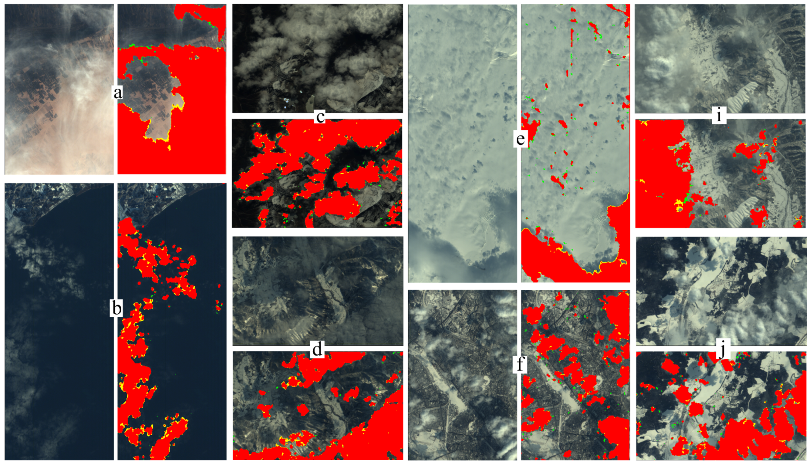
Figure 7 shows the cloud detection results for different terrains. We can see that a sheer visual comparison of the results and the false colour composites shows that the algorithm developed in this study scored favourable achievements when detecting cloud pixels. Figure 7a represents a summer image of cirrostratus over desert acquired on 8 August 2013. The detection results reveal that the proposed algorithm is well qualified in excluding clouds from desert, even though the clouds were so thin that their spectra were mixed with that of the desert pixels. Figure 7b is a winter image acquired on 3 June 2013 of dark stratus over the ocean and coast. Clouds contain water droplets that have the same materials as the ocean in that season; however, water in the ocean is in the form of liquid, and water in clouds is in the form of an aerosol. The spectra of the same material is differ as form or temperature differs. The omission error rate were approximately 1.73% in the yellow region, which is different from manually labelled cloud mask of the border of the thin clouds. Figure 7c shows an image of cumulus and stratocumulus acquired at noon in the spring on 22 May 2012 around the Himalayan mountains, and Figure 7d shows an image of altocumulus over mountains acquired at dusk in the winter on 3 January 2007, the omission error rate of which was 0.62%. Compared with Figure 7d, Figure 7c seems to show lighter due to the smaller sun zenith angle. However, both images show favourable cloud detection results, even if the darkened clouds can also be detected. Figure 7f shows an image of cumulus over Haerbin, Heilongjiang Province acquired on 28 March 2005. Given that both the freezing river and city highlights were classified as clouds, there was approximately 0.23% commission errors. In the suspected cloud region, there was 0.16% omission errors. Figure 7e,i,j show images of clouds over snow or ice. The image of stratocumulus clouds over a snowfield in the cryosphere shown in Figure 7e was acquired on 12 May 2012, and approximately 4.8% of cloud pixels in the entire image are indistinguishable by the naked eye. These pixels are floating over the snow field. The commission error rate was 0.41% when compared with the classification of the manually labelled cloud mask. Figure 7i presents a spring image acquired on 17 March 2007 of altostratus clouds over a snow-covered mountain. Because altostratus clouds lack clear outlines in visible bands, the edges of the altostratus clouds look quite similar to the ground edges. Although approximately 2.97% of the cloud pixels are hard to distinguish by the naked eye in the visible bands, they were properly classified using the proposed method. The spring image shown in Figure 7j, which was obtained on 28 March 2005, shows cumulus clouds over a forest covered by frozen lake. Most of the cumulus clouds are floating over the ice. They share 0.21% of the omission errors.
4.4. Cloud Detection Performance of Each Stage
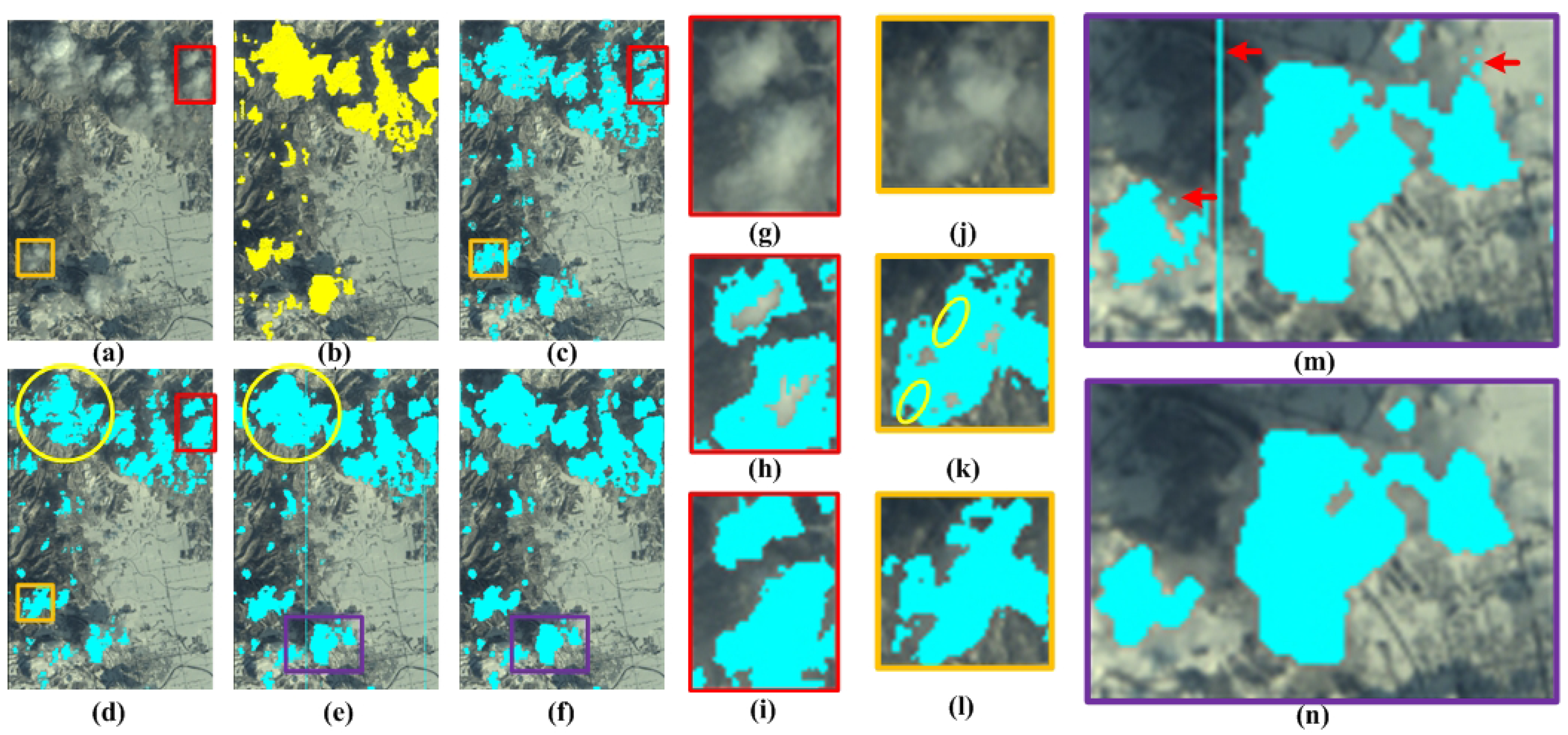
Depicting the cloud condition of EO-1 Hyperion images from four different states, Figure 8 presents the performance of the proposed algorithm performance at each processing stage. By visually comparing the results with the false colour composites, we observe that there were FN classifications in the light cloud region under the TDT method because various reflectances shared fixed parameters, as shown in Figure 8h. Contrarily, TESAM was able to correctly classify the cloud regions that were misclassified under the TDT method, as shown in Figure 8i. In addition, various reflectances did not exert much influence over cloud detection. Compared with TDT, TESAM seems to be conservative, abstaining from ambiguous classification to prevent mixtures of heterogeneous spectra for the aMRF procedure. The ambiguous classification is shown in the yellow circle of Figure 8k. These region were not labelled as clouds under TESAM, as shown in Figure 8l. After TESAM detection, the cloud regions detected using TESAM worked as seed regions during aMRF. By comparing the yellow circles of Figure 8d,e, we can identify that after aMRF detection, some cloud regions grew more fuller. In addition, because aMRF is fault-tolerant, the TN regions regained to ground pixels. Detailed introduction of the iterative process of aMRF will be presented later. Nevertheless, the spectra of some individual pixels were quite similar to those of clouds under selected bands for aMRF. Therefore, even if the neighbours’ contributions were considered, the energy of those pixels under aMRF remained weak. Those cloud mask pixels were taken as noisy points by DSR. A comparison of Figure 8m,n uncovers that DSR turned the binary properties of those noisy points over. As presented in Figure 8n, the vertical line and some isolated pixels in Figure 8m were eliminated after DSR processing.
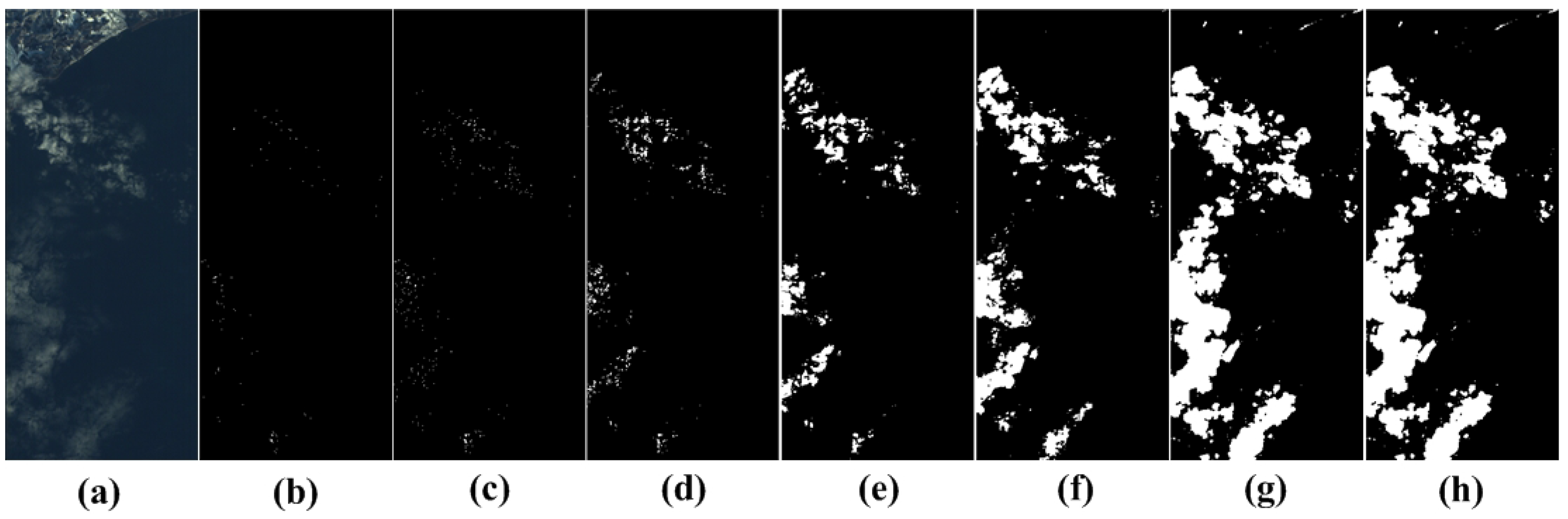
A detailed example of the aMRF iterative process is shown in Figure 9. The cloud regions that were detected using the TDT method and TESAM were rather limited (0.02% and 0.12% of TP were within 18.3% of the actual cloud cover content). Only a few detected cloud pixels existed in the mask, as seen in Figure 9a,b. The TESAM detection result was treated as an initial classification for aMRF. Comparing Figure 9c–h, the aMRF method was obviously strongly robust when the spectrum of the initial seed region (seed region) was pure enough. The initial classification of each time of iteration was the result of the previous iteration, and after the 8th iteration, the classification was in good agreement with the real cloud region. In addition, the image tended to be convergent at the 16th iteration.
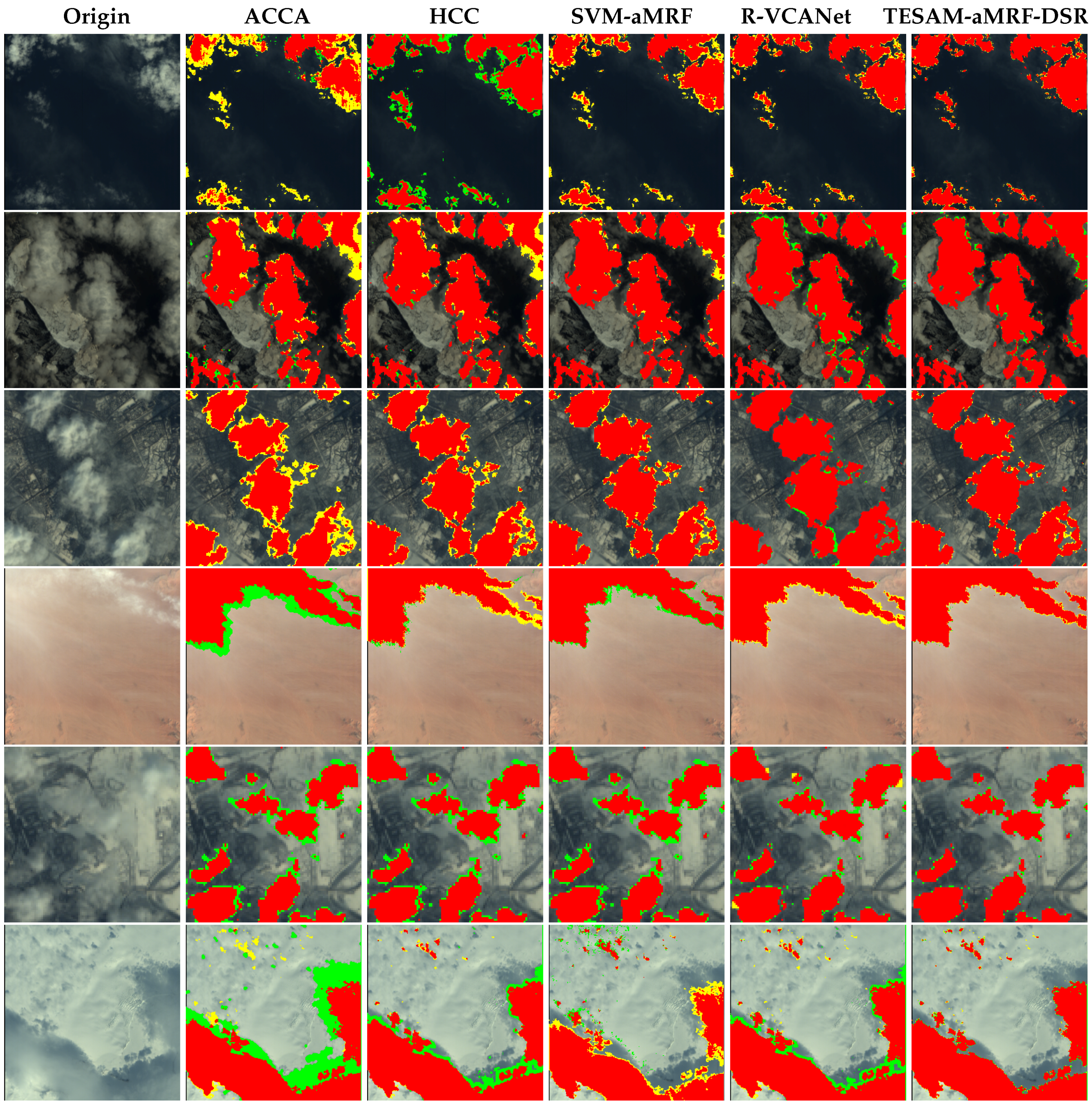
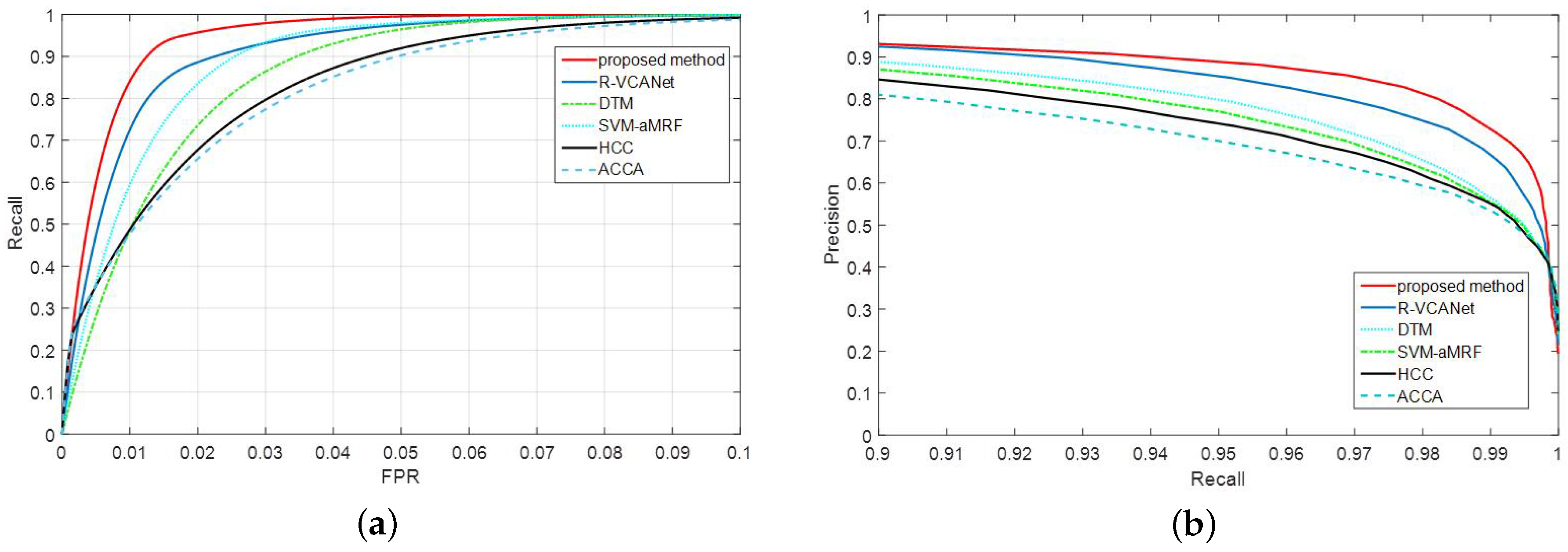
Figure 10 shows a comparison of the cloud detection performance of some methods. The terrains from the first row to the last row are ocean, mountain, city, desert, ice and cryosphere. It can be observed that the proposed method produced the best precision ratio and recall ratio and its error was lower thatn those of the other methods. ACCA had high FN for ordinary terrain and high FP for special terrain due to the lack of the thermal infrared band. HCC had difficulty detecting thin or dark clouds. The Decision Theoretical Method(DTM) classified the majority of the thin clouds as ground. It had a high FP under DTM. The support vector machine adaptive Markov random field (SVM-aMRF) and rolling guidance filter and vertex component analysis network(R-VCANet) had higher recall ratios and precision ratios than those of the previous two. Nevertheless, they still produced classification errors for thin clouds primarily because thin clouds are mixed with other spectra that cannot be learned sufficiently. The ROC and precision/recall curves are shown in Figure 11 and Figure 12.
5. Discussions
5.1. The Effectiveness of Combining the Threshold Decision Tree and Spectral Angle Map
Spectral Angle Maps are widely used due to their simplicity and geometrical interpretability. SAMs are invariant to the (unknown) multiplicative scaling of spectra due to differences in illumination and angular orientation. The invariance of multiplicative scaling constitutes one of the most important properties of spectral angle distance. Due to the invariant nature of angles among linearly scaled variations, the spectral angle between two pixels is more sensitive to the shape of the spectral signatures than absolute intensities. Traditional TDT methods sometimes overestimate or underestimate cloud regions because fixed parameters were unsuitable for changing illumination and angular orientation. In theory, the TESAM method could reduce the misclassification.
5.2. The Usefulness of Spatial Information for Cloud Detection
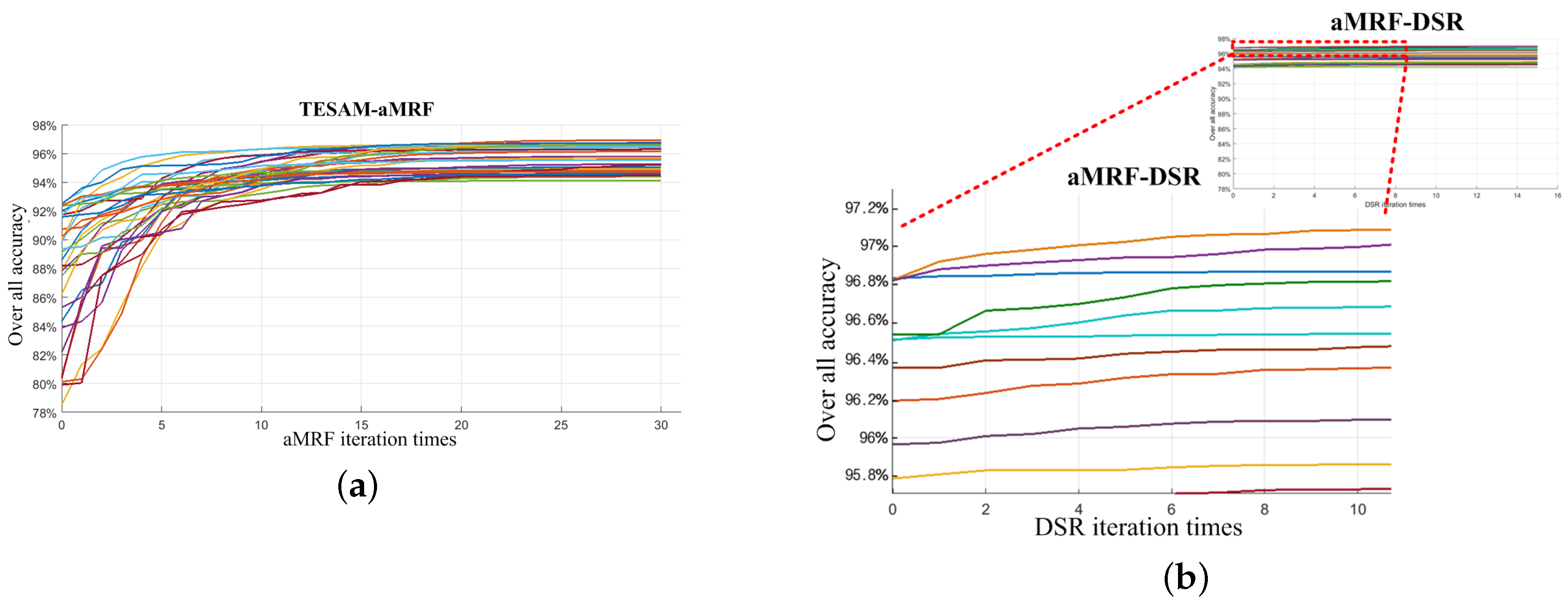
For still existing wrong classification pixels after TESAM, aMRF was used to employed all the spectral and spatial information into an energy index to identify the class attribute at the regional scales. In general, the optimal status was recorded when the energy was stable, and the iteration was then terminated accordingly. The aMRF mainly chose vapour reflection bands (1.38 μm∼1.39 μm and 1.46 μm∼1.55 μm). Although the spectra of thin cloud pixels and dark cloud pixels deviated from the threshold, aMRF was able to again recognize those cloud pixels. The cloud mask from aMRF contained noisy points because the data processed onboard were level 0.5 and had not been fully calibrated. The radiance and reflectance values for level 0.5 SWIR bands should be considered as pseudo-radiances and pseudo-reflectances. DSR could eliminate those noisy points in the binary mask, which is a refinement process for cloud detection. The iteration results for the aMRF and DSR detection accuracies are presented in Figure 12, for which we randomly selected parts of the dateset. The aMRF iteration accuracy each time results is shown in Figure 12a. The 0th iteration represents the overall accuracy of TESAM. During aMRF iteration, the detection accuracy increased more or less each time. The differing improvements in the level of detection accuracy under aMRF iteration resulted primarily from cloud conditions. The termination condition for aMRF iteration was that the rate of pixel attributes changed over two adjacent iterations was within 0.5% of the overall pixels. The DSR iteration accuracy is shown in Figure 12b. The 0th iteration represents the overall accuracy of aMRF. During the DSR iteration, the accuracy of each iteration increased slightly, yet it eliminated numerous isolated noise-points, greatly benefiting ROI compression. The DSR iteration termination condition was that the rate of pixel attributes changed over two adjacent iterations was within 0.005% of the overall pixels.
5.3. Error Sources of the Proposed Method
In brief, the cloud detection results uncover that the proposed method scored favourable achievements when detecting clouds in EO-1 images. However, two sources of error that might influence algorithm accuracy should also be noted. The first is that the cloud region detected using the TDT algorithm was larger than its actual size, which may have resulted from unsuitable parameters. Correspondingly, TESAM overestimated the area of the cloud region in that the size of the cloud region was jointly by TDT and TESAM histogram. In that manner, the FPR region of TESAM results was also increased because impure cloud spectra may lead to classification errors for large areaa under aMRF. The second is that the selected bands for aMRF might not be the best choice for all types of surface features. In this case, the advantage of high spectral purity in the seed region will be lost when the contribution from the neighbour is insufficient.
5.4. Effect of Compression Based on Cloud Detection
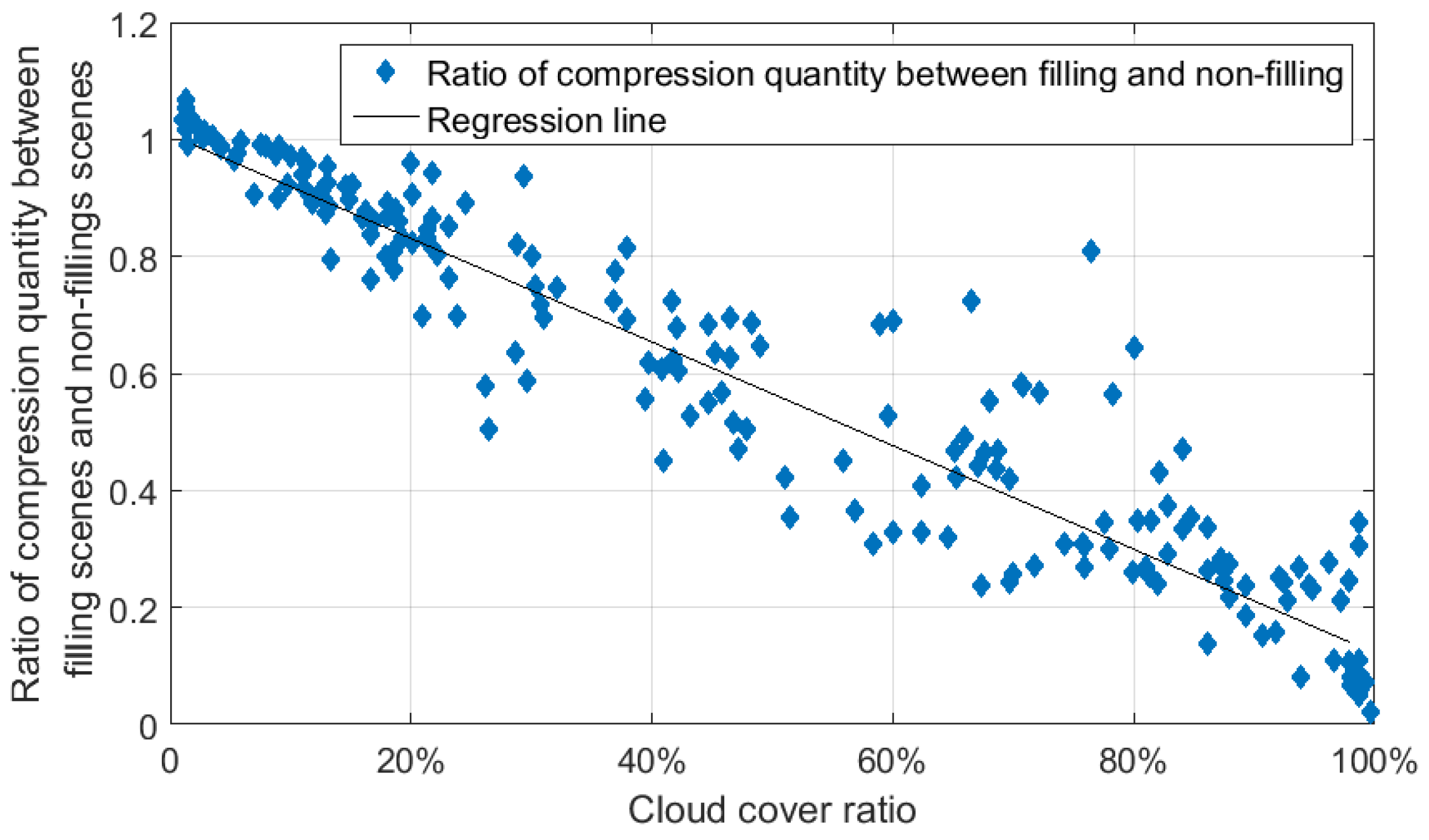
The compression effect is worth mentioning. The cloud region is filled by optimal values after obtaining the cloud mask, and the cloud region data can then be removed through compression. For a Hyperion image with a cloud cover rate 30.12%, the data size of the filled-value compression is 71.27% of that for the original lossless compression. The difference between the lossless compression ratios for the ground and clouds should be considered, and non-filling cloud regions contribute less to compression than the filled cloud regions. According to statstics, the relationship between compression quantity and cloud ratios is shown in Figure 13. The regression line reveals that the ratio of compression data volumes between filled and non-filled cloud regions is approximately proportional to the cloud cover ratio. The tendency shapes linear. In addition, the closer it gets to 1:1, the better the compression performance of filling-value is. Certain points exceeding 1 indicate that those scenes contained small thin clouds, whereas some points close to zero revealed that the scene was completely covered by cloud.
5.5. Applicability of the Developed Methods in the Feature
The proposed method is highly automatic and efficient when processing huge volumes of real-time images. It can easily be implemented on parallel processors, such as FPGAs. External storage devices or architectures such as ping-pong structures are in demand because they can restore data for supporting the use of spatial context. Moreover, classifiers instantiated in hardware logic have achieved in the implementation of arccosine [47], exponentials [48,49] functions, and even floating-point operations, supporting numerous classifiers and the simple operations of nonlinear classifiers. Additionally, real-time for processing is required. The bandwidth of multi DDRs could satisfy Gb/s algorithm throughputs using a small fixed number of arithmetic operations on locally available data. The proposed method can also be applied to images acquired by similar satellite instruments that have similar spectral bands and temporal resolutions. The method presented in this paper is general and further tests will be conducted in other regions with different environments.
6. Conclusions
TESAM-aMFR-DSR is an innovative approach for onboard cloud detection. Different from classical hyperspectral cloud detection algorithm, the proposed method combines TDT with ESAM. As the initial seed region of cloud for aMRF, it improves spectral purity. The aMRF method uses an energy index by combining spectral features with spatial information. It is robust to shadowed regions of clouded areas, thin clouds and misclassified ground pixels. There are noisy points that are misclassified during the aMRF process due to the use of onboard processing data that are not fully calibrated. DSR then eliminates those noisy points using a double-well model. The cloud detecion results obtained in this study demonstrate the performance of the proposed method. The performances of this method were evaluated using EO-1/Hyperion images. Agreements were found between detection results and a manually labelled image, with an overall accuracy of 96.28%. By using spatial information, approximately 8.35% of the misclassified cloud pixels from the initial spectral tests were excluded. The compression quantity ratio between the filled and non-filled scenes is approximately proportional to cloud cover ratio. The tendency is linear. Filled cloud regions improve compression performance. In conclusion, the proposed method exhibited high accuracy for clouds recognition using EO-1 Hyperion images and was an improvement over traditional spectral-based algorithms. The proposed method can also be adapted for images acquired by the satellite instruments with similar spectral bands and temporal resolutions.
Acknowledgments
Project supported by the National Nature Science Foundation of China (No. 60543006). The authors would like to thank the editor and reviewers for their instructive comments that helped to improve this manuscript. Besides, they would also like to thank the international scientific data service platform and the U.S. Geological Survey website.
Author Contributions
Haoyang Li, Hong Zheng and Chuanzhao Han conceived of the study and designed the experiments; Haibo Wang and Min Miao took part in the research and analyzed the data; Haoyang Li wrote the main program and most of the paper.
Conflicts of Interest
The authors declare no conflict of interest.
Abbreviations
The following abbreviations are used in this manuscript:
| ACCA | Automatic Cloud Cover Algorithm |
| aMRF | adaptive Markov Random Field |
| CC | Cloud Cover |
| DCC-ASE | Detection of Cryospheric Change Automonous Sciencecraft Experiment |
| DSR | Dynamic Source Resonance |
| DTM | Decision Theoretic Method |
| EO-1 | Earth Observing-1 |
| ESAM | Exponential Spectral Angle Map |
| FL | Fast Lossless |
| FN | False Negative |
| FP | False Positive |
| FPR | False Positive Rate |
| HCC | Hyperion Cloud Cover |
| HSI | Hyperspectral Image |
| LUT | Look Up Table |
| MRF | Markov Random Field |
| MODIS | Moderate-resolution Imaging Spectroradiometer |
| NAPC | Noise-adjusted Principle Components |
| NDSI | Normalized Difference Snow Index |
| NIR | Near Infrared |
| ROC | Receiver Operating Characteristic Curve |
| ROI | Region of Interest |
| R-VCANet | Rolling Guidance filter and Vertex Component Network |
| SAM | Spectral Angle Map |
| SVM | Support Vertor Machine |
| SVM-aMRF | Support Vector Machine adaptive Markov Random Field |
| TDT | Threshold Decision Tree |
| TESAM | Threshold assisted Exponential Spectral Angle Map |
| TIR | Thermal Infrared |
| TN | True Negative |
| TOA | Top of Atmosphere |
| TP | True Positive |
| USGS | United States Geological Survey |
| VNIR | Visible and Near Infrared |
| VSWIR | Visible and Short Wave Infrared |
| WMO | World Meteorological Organization |
Appendix A Some Parameters for Meteorological Satellite and Earth Observation Satellite

Table A1.
Meteorological satellite vs. Earth observation satellite.
| Satellite | The Used Sensor | Image Resolution | Data Size | Download Speed | |
|---|---|---|---|---|---|
| Meteorological satellite | FY-3A | MERSI | 1100 m | 4GB | 93 Mb/s |
| Noaa18 | AVHRR | 1100 m | / | 138 Mb/s | |
| GMS-5 | VISSR | 1250 m | / | 14 Mb/s | |
| Meteosat | VISSR | 1000 m | / | 3.2 Mb/s | |
| Meteor-m2 | KMSS | 1000 m | / | 665 kb/s | |
| Earth observation satellite | EO-1 | Hyperion | 30 m | / | 120 Mb/s |
| NEMO(HRST) | AVIRIS | 20 m | 227 GB | 150 Mb/s | |
| QuickBird | QuickBird | 0.6 m | 128 GB | 320 Mb/s | |
| LANDSAT8 | OLI/TIRS | 15 m | 400 GB | 330 Mb/s | |
| EROS B1 | Panchromatic | 0.82 m | / | 280 Mb/s | |
| Resurs dk1 | ESI | 1 m | 768 GB | 330 Mb/s |
Appendix B Pseudocode for the TESAM Model
| Algorithm A1 TDT assisted ESAM |
| Input: the remote sensing image data I with K pixels, each pixel is N-dimentional spectral vectors X=, the referenced spectrum Y= |
| Output: the class labels map M |
| step1: |
| for k=1 to K do |
| = ( computes the exponential spectral angle according to Equations(1)-(3)). |
| end |
| for k=1 to K do |
| = ( computes the number of cloud pixels according to TDT) |
| end |
| step2: |
| Computes the histogram of |
| step3: |
| for k=1 to n do |
| = ( computes the threshold for ESAM according to Equations(4)-(5)) |
| end |
| Step4: |
| for k=1 to K do |
| = ( determine the binary class label according to Equations(6)) |
| end |
Appendix C Pseudocode for the aMRF Model
| Algorithm A2 TESAM-aMRF |
| Input: the remote sensing image data I with K pixels, each pixel is n-dimentional spectral vectors X = , the referenced spectrum Y=, the class labels map M. |
Output: the class labels map M
|
Appendix D Pseudocode for the DSR Model
| Algorithm A3 aMRF-DSR |
| Input: the class labels M |
| Output: the class labels M |
| step1: |
| for k=1 to K do |
| (M(k)=cloud), (M(k)=ground) ( computes the pixel number of 8-neighborhood around pixel k that belongs to ground and cloud respectively); |
| compare and , designating the number of bigger one to ; |
| Refresh x according to Equations (12)-(13); |
| end |
| step2: Refresh M |
| step3: Iterate the procedure of step1-step2; |
References
- Li, W.; Wu, G.; Zhang, F.; Du, Q. Hyperspectral Image Classification Using Deep Pixel-Pair Features. IEEE Trans. Geosci. Remote Sens. 2017, 55, 645–657. [Google Scholar] [CrossRef]
- Kinter, J.L.; Shukla, J. The Global Hydrologic and Energy Cycles: Suggestions for Studies in the Pre-Global Energy and Water Cycle Experiment (GEWEX) Period. Bull. Am. Meteorol. Soc. 2013, 71, 181–271. [Google Scholar] [CrossRef]
- Shen, H.; Pan, W.D.; Wu, D. Predictive lossess compression of regions of interest in hyperspectral images with no-data regions. IEEE Trans. Geosci. Remote Sens. 2016, 55, 173–182. [Google Scholar] [CrossRef]
- Shen, H.; Pan, W.D. Predictive Lossless Compression of Regions of Interest in Hyperspectral Image Via Correntropy Criterion Based Least Mean Square Learning. In Proceedings of the IEEE International Conference on Image Processing, Phoenix, AZ, USA, 25–28 September 2016. [Google Scholar]
- Mandrake, L.; Frankenberg, C.; O’Dell, C.W.; Osterman, G.; Wennberg, P.; Wunch, D. Semi-autonomous sounding selection for OCO-2. Atmosp. Meas. Tech. Discuss. 2013, 6, 5881–5922. [Google Scholar] [CrossRef]
- Chien, L.S.; Mclaren, D.; Tran, D.; Davies, A.G.; Doubleday, J.; Mandl, D. Onboard product generation on earth observing one: A pathfinder for the proposed HyspIRI mission intelligent payload module. IEEE J. Sel. Top. Appl. Earth Obs. Remote Sens. 2013, 6, 257–264. [Google Scholar] [CrossRef]
- Xu, X.; Yuan, C.; Liang, X.; Shen, X. Rendering and Modeling of Stratus Cloud Using Weather Forecast Data. In Proceedings of the IEEE International Conference on Virtual Reality and Visualization, Fujian, China, 17–18 October 2015. [Google Scholar]
- King, M.D.; Platnick, S.; Menzel, W.P.; Ackerman, S.A.; Hubanks, P.A. Spatial and temporal distribution of clouds observed by MODIS onboard the Terra and Aqua satellites. IEEE Trans. Geosci. Remote Sens. 2013, 51, 3826–3852. [Google Scholar] [CrossRef]
- Cadau, E.; Laneve, G. Improved MSG-SEVIRI images cloud masking and evaluation of its impact on the fire detection methods. In Proceedings of the IEEE International Conference on Geoscience and Remote Sensing Symposium, Boston, MA, USA, 6–11 July 2008. [Google Scholar]
- Shen, H.; Pan, W.D.; Wang, Y. A Novel Method for Lossless Compression of Arbitrarily Shaped Regions of Interest in Hyperspectral Imagery. In Proceedings of the IEEE Southeast Conference, Fort Lauderdale, FL, USA, 9–12 April 2015. [Google Scholar]
- Mercury, M.; Green, R.; Hook, S.; Oaida, B.; Wu, W.; Gunderson, A.; Chodas, M. Global cloud cover for assessment of optical satellite observation opportunities: A HyspIRI case study. Remote Sens. Environ. 2012, 126, 62–71. [Google Scholar] [CrossRef]
- Conoscenti, M.; Coppola, R.; Magli, E. Constant SNR, Rate Control, and Entropy Coding for Predictive Lossy Hyperspectral Image Compression. IEEE Trans. Geosci. Remote Sens. 2016, 54, 7431–7441. [Google Scholar] [CrossRef]
- Mat Noor, N.R.; Vladimirova, T. Investigation into lossless hyperspectral image compression for satellite remote sensing. Int. J. Remote Sens. 2013, 34, 5072–5104. [Google Scholar] [CrossRef]
- Nian, Y.; Xu, K.; Wan, J.; Wang, L.; He, M. Block-based KLT compression for multispectral images. Int. J. Wavel. Multiresolut. Inf. Process. 2016, 14. [Google Scholar] [CrossRef]
- Wang, L.; Wu, J.; Jiao, L.; Shi, G. Lossy-to-Lossless Hyperspectral Image Compression Based on Multiplierless Reversible Integer TDLT/KLT. IEEE Geosci. Remote Sens. Lett. 2009, 6, 587–591. [Google Scholar] [CrossRef]
- Gonzalez-Conejero, J.; Bartrina-Rapesta, J.; Serra-Sagrista, J. JPEG 2000 encoding of remote sensing multispectral images with no-data regions. IEEE Geosci. Remote Sens. Lett. 2010, 7, 251–255. [Google Scholar] [CrossRef]
- Li, H.; Zheng, H.; Han, C. Adaptive run-length encoding circuit based on cascaded structure for target region data extraction of remote sensing image. In Proceedings of the International Conference on Integrated Circuits and Microsystems, Chengdu, China, 25–28 November 2016. [Google Scholar]
- El-Araby, E.; Taher, M.; El-Ghazawi, T.; Le Moigne, J. Prototyping automatic cloud cover assessment (ACCA) algorithm for remote sensing on-board processing on a reconfigurable computer. In Proceedings of the IEEE International Conference on Field-Programmable Technology, Singapore, 11–14 December 2005. [Google Scholar]
- Gao, X.J.; Wan, Y.C.; Zheng, X.Y. Real-Time automatic cloud detection during the process of taking aerial photographs. Spectrosc. Spectr. Anal. 2014, 34, 1909–1913. [Google Scholar]
- Ackerman, S.A.; Strabala, K.I.; Menzel, W.P.; Frey, R.A.; Moeller, C.C.; Gumley, L.E. Discriminating clear sky from clouds with MODIS. J. Geophys. Res. Atmosp. 1998, 103, 32141–32157. [Google Scholar] [CrossRef]
- Ackerman, S.A.; Holz, R.E.; Frey, R.; Eloranta, E.W.; Maddux, B.C.; McGill, M. Cloud detection with MODIS. Part II: Validation. J. Atmosp. Ocean. Technol. 1998, 103, 1073–1086. [Google Scholar] [CrossRef]
- Frey, R.A.; Ackerman, S.A.; Liu, Y.; Strabala, K.I.; Zhang, H.; Key, J.R.; Wang, X. Cloud detection with MODIS. Part I: Improvements in the MODIS cloud mask for collection 5. J. Atmosp. Ocean. Technol. 2008, 25, 1057–1072. [Google Scholar] [CrossRef]
- Wei, J.; Sun, L.; Jia, C.; Yang, Y.; Zhou, X.; Gan, P.; Jia, S.; Liu, F.; Li, R. Dynamic threshold cloud detection algorithms for MODIS and Landsat 8 data. In Proceedings of the IEEE International Geoscience and Remote Sensing Symposium, Beijing, China, 10–15 July 2016. [Google Scholar]
- Griggin, M.; Burke, H.H.; Mandl, D.; Miller, J. Cloud cover detection algorithm for EO-1 hyperion imagery. In Proceedings of the 17th SPIE AeroSense Conference on Algorithms Technology Multispectral, Hyperspectral Ultraspectral Imagery IX, Orlando, FL, USA, 21–25 July 2003. [Google Scholar]
- Doggett, T.; Greeley, R.; Chien, S.; Castano, R.; Cichy, B.; Davies, A.G.; Rabideau, G.; Sherwood, R.; Tran, D.; Baker, V.; et al. Autonomous on-board detection of cryospheric change with Hyperion on-board Earth Observing-1. Remote Sens. Environ. 2006, 101, 447–462. [Google Scholar] [CrossRef]
- Ip, F.; Dohm, J.M.; Baker, V.R.; Doggett, T.; Davies, A.G.; Castano, R.; Chien, S.; Cichy, B.; Greeley, R.; Sherwood, R.; et al. Flood detection and monitoring with the autonomous sciencecraft experiment onboard EO-1. Remote Sens. Environ. 2006, 101, 463–481. [Google Scholar] [CrossRef]
- Irish, R.R. Landsat 7 automatic cloud cover assessment. Algorithms for Multispectral, Hyperspectral, and Ultraspectral Imagery. In Proceedings of the International Society for Optical Engineering, Orlando, FL, USA, 24 April 2000. [Google Scholar]
- Wang, M.; Shi, W. Cloud masking for ocean color data processing in the coastal regions. IEEE Trans. Geosci. Remote Sens. 2006, 44, 3105–3196. [Google Scholar] [CrossRef]
- Deng, J.; Wang, H.; Ma, J. An Automatic cloud detection algorithm for Landsat Remote Sensing Image. In Proceedings of the 4th International Workshop on Earth Observation and Remote Sensing Applications, Guangdong, China, 11–14 December 2016. [Google Scholar]
- Gómez-Chova, L.; Camps-Valls, G.; Calpe-Maravilla, J.; Guanter, L.; Moreno, J. Cloud-screening algorithm for ENVISAT/MERIS multispectral images. IEEE Trans. Geosci. Remote Sens. 2007, 45, 4105–4118. [Google Scholar] [CrossRef]
- Taylor, T.E.; O’Dell, C.W.; O’Brien, D.M.; Kikuchi, N.; Yokota, T.; Nakajima, T.Y.; Ishida, H.; Crisp, D.; Nakajima, T. Comparison of cloud-screening methods applied to GOSAT near-infrared spectra. IEEE Trans. Geosci. Remote Sens. 2012, 50, 295–309. [Google Scholar] [CrossRef]
- Minnis, P.; Trepte, Q.Z.; Sun-Mack, S.; Chen, Y.; Doelling, D.R.; Young, D.F.; Spangenberg, D.A.; Miller, W.F.; Wielicki, B.A.; Brown, R.R.; et al. Cloud detection in nonpolar regions for CERES using TRMM VIRS and terra and aqua MODIS data. IEEE Trans. Geosci. Remote Sens. 2008, 46, 3857–3884. [Google Scholar] [CrossRef]
- Lee, J.; Weger, R.C.; Sengupta, S.K.; Welch, R.M. A neural network approach to cloud classification. IEEE Trans. Geosci. Remote Sens. 1990, 28, 846–855. [Google Scholar] [CrossRef]
- Martins, J.V.; Tanré, D.; Remer, L.; Kaufman, Y.; Mattoo, S.; Levy, R. MODIS cloud screening for remote sensing of aerosols over oceans using spatial variability. Geophys. Res. Lett. 2002, 29, MOD4-1–MOD4-4. [Google Scholar] [CrossRef]
- Bian, J.; Li, A.; Liu, Q.; Huang, C. Cloud and Snow Discrimination for CCD Images of HJ-1A/B Constellation Based on Spectral Signature and Spatio-Temporal Context. Remote Sens. 2016, 8, 31. [Google Scholar] [CrossRef]
- Murtagh, F.; Barreto, D.; Marcello, J. Decision boundaries using Bayes factors. IEEE Trans. Geosci. Remote Sens. 2003, 41, 2952–2958. [Google Scholar] [CrossRef]
- Yu, H.; Gao, L.; Li, J.; Li, S.S.; Zhang, B.; Benediktsson, J.A. Spectral-Spatial Hyperspectral Image Classification Using Subspace-Based Support Vector Machines and Adaptive Markov Random Fields. Remote Sens. 2016, 8, 355. [Google Scholar] [CrossRef]
- Merchant, C.J.; Harris, A.R.; Maturi, E.; MacCallum, S. Probabilistic physically based cloud screening of satellite infrared imagery for operational sea surface temperature retrieval. Q. J. R. Meteorol. Soc. 2005, 131, 2735–2755. [Google Scholar] [CrossRef] [Green Version]
- Thompson, D.R.; Green, R.O.; Keymeulen, D.; Lundeen, S.K.; Mouradi, Y.; Nunes, D.C.; Castaño, R.; Chien, S.A. Rapid Spectral Cloud Screening Onboard Aircraft and Spacecraft. IEEE Trans. Geosci. Remote Sens. 2014, 52, 6779–6792. [Google Scholar] [CrossRef]
- Pan, B.; Shi, Z.; Xu, X. R-VCANet: A New Deep-Learning-Based Hyperspectral Image Classification Method. IEEE J. Sel. Top. Appl. Earth Obs. Remote Sens. 2017, 10, 1975–1986. [Google Scholar] [CrossRef]
- Scaramuzza, P.L.; Bouchard, M.A.; Dwyer, J.L. Development of the Landsat Data Continuity Mission Cloud-Cover Assessment Algorithms. IEEE Trans. Geosci. Remote Sens. 2012, 50, 1140–1157. [Google Scholar] [CrossRef]
- Liu, J. Improvement of dynamic threshold value extraction technic in FY-2 cloud detection. J. Infrared Millim. Waves 2010, 29, 288–292. [Google Scholar]
- Chang, C.-I.; Du, Q. Interference and noise-adjusted principal components analysis. IEEE Trans. Geosci. Remote Sens. 1999, 37, 2387–2396. [Google Scholar] [CrossRef]
- Tarabalka, Y.; Benediktsson, J.A.; Chanussot, J. Spectral-spatial classification of hyperspectral imagery based on partitional clustering techniques. IEEE Trans. Geosci. Remote Sens. 2009, 47, 2973–2987. [Google Scholar] [CrossRef]
- Hergert, W.; Wriedt, T. Mie theory: A review. In The Mie Theory; Springer: Berlin, Germany, 2012; Volume 169, pp. 53–71. [Google Scholar]
- Yang, P.; Bi, L.; Baum, B.A.; Liou, K.N.; Kattawar, G.W.; Mishchenko, M.I.; Cole, B. Spectrally consistent scattering, absorption, and polarization properties of atmospheric ice crystals at wavelengths from 0.2 to 100 μm. J. Atmos. Sci. 2013, 70, 330–347. [Google Scholar] [CrossRef]
- Dongmei, H.H.Z.J.W.; Yongyi, L.N.Q. Implementation of Arccosine Function Based on FPGA. Electron. Technol. 2013, 6, 5–8. [Google Scholar]
- Tang, W.; Liu, G. FPGA Fixed-Point Technology of Exponential Function Achieved by CORDIC Algorithm. J. South China Univ. Technol. 2016, 44, 9–14. [Google Scholar]
- Malík, P. High throughput floating point exponential function implemented in FPGA. In Proceedings of the IEEE Computer Society Annual Symposium on VLSI, Montpellier, France, 8–10 July 2015. [Google Scholar]
Figure 1.
Cloud detection results under the TDT method. (a) Original image; (b) spectra of thick clouds, thin clouds and surface features that were sampled from red, blue and green crosses in (a); (c) Two scenes that contain liquid clouds, mixed phase clouds, ice clouds and snow, which are labelled in the figure; (d) spectra of liquid clouds, mixed phase clouds, ice clouds and snow sampled from the regions in the boxes of (c) correspondingly; (e) cloud detection results under the TDT method (red denotes the extracted correct cloud region, yellow denotes the omission errors and green denotes the commission errors); (f) Diagrammatic sketch of the misclassification of ground and cloud pixels under TDT method.

Figure 2.
Spectral curve statistics of cloud and ground reflectance. (a) Normalized spectral reflectance curve of different cloud types; (b) Normalized spectral reflectance curve of different materials.
Figure 2.
Spectral curve statistics of cloud and ground reflectance. (a) Normalized spectral reflectance curve of different cloud types; (b) Normalized spectral reflectance curve of different materials.

Figure 3.
General framework and flowchart of the proposed method. (a) General framework of the proposed method; (b) all the models of the proposed method and flowchart.
Figure 3.
General framework and flowchart of the proposed method. (a) General framework of the proposed method; (b) all the models of the proposed method and flowchart.

Figure 4.
combination of ESAM with TDT.

Figure 5.
SR in a double-well potential valley.

Figure 6.
Test dataset description. (a) Geographical distribution of the selected scene; (b) Distribution of seasons for the selected scene; (c) Time distribution of the selected scene; (d) Number of Scenes for each terrain.
Figure 6.
Test dataset description. (a) Geographical distribution of the selected scene; (b) Distribution of seasons for the selected scene; (c) Time distribution of the selected scene; (d) Number of Scenes for each terrain.

Figure 7.
Cloud detection results for different kinds of ground. (a) Desert with thin cirrostratus and cloud detection result; (b) Ocean with dark stratus and cloud detection result; (c) Mount Qomolangma with stratocumulus and cloud detection result; (d) Mountain with dark altocumulus and cloud detection result; (e) Snow cover with straocumulus and cloud detection result; (f) Highlight city with frozen lake scene and cloud detection result; (i) Mountain with thin altostratus and cloud detection result; (j) Frozen field with cumulus and cloud detection result. (Red denotes extracted correct cloud regions (TP), yellow denotes missed cloud regions (omission errors/FN) and green denotes non-cloud regions misjudged as cloud regions (commission errors/FP)).

Figure 8.
Comparison of cloud detection results. (a) A winter image acquired on 7 December 2013, with obvious clouds over the entire image; (b) Manually labelled image result; (c) Cloud detection result using TDT method; (d) Cloud detection result using the TESAM method; (e) Cloud detection based on; (d) using the aMRF method; (f) Cloud detection based on (e) using DSR; (g–i) show the original picture, TDT labelled and TESAM labelled images of the cloud region respectively. (g–i) correspond to the red boxes in (a,c,d) respectively; (j–l) correspond to the original picture, TDT labelled and TESAM labelled iamges of cloud region respectively.(j–l) correspond to the orange boxes in (a,c,d) respectively; (m) is the result of aMRF processing and corresponds to the purple box in (e); and (n) was processed using DSR based on (e) and corresponds to the purple box in (f).

Figure 9.
The detailed aMRF iteration results. (a) Original image; (b) TESAM classification result ; (c–h) The 1st, 2nd, 4th, 8th, 16th and 30th aMRF iteration results respectively.
Figure 9.
The detailed aMRF iteration results. (a) Original image; (b) TESAM classification result ; (c–h) The 1st, 2nd, 4th, 8th, 16th and 30th aMRF iteration results respectively.

Figure 10.
Cloud detection performance comparasion. (Red denotes the extracted correct cloud regions (TP), yellow denotes the missed cloud regions (omission error/FN) and green denotes the non-cloud regions misjudged as cloud regions (commission error/FP)).
Figure 10.
Cloud detection performance comparasion. (Red denotes the extracted correct cloud regions (TP), yellow denotes the missed cloud regions (omission error/FN) and green denotes the non-cloud regions misjudged as cloud regions (commission error/FP)).

Figure 11.
Comparison of the performances of the different algorithms. (a) ROC curve of cloud detection performance for each method; (b) Precision performance curves corresponding to recall for each method.
Figure 11.
Comparison of the performances of the different algorithms. (a) ROC curve of cloud detection performance for each method; (b) Precision performance curves corresponding to recall for each method.

Figure 12.
Statistics of each iteration results of aMRF and DSR. (a) over all accuracy of aMRF iteration results; (b) over all accuracy of DSR iteration results.
Figure 12.
Statistics of each iteration results of aMRF and DSR. (a) over all accuracy of aMRF iteration results; (b) over all accuracy of DSR iteration results.

Figure 13.
Statistics of cloud cover and ratio of compression quantity between filled and non-filled cloud regions.
Figure 13.
Statistics of cloud cover and ratio of compression quantity between filled and non-filled cloud regions.

Table 1.
Spectrum used by threshold methods and disadvantage.
| Method | Spectra Utilized | Disadvantage |
|---|---|---|
| ACCA [41] | 0.45–0.52 μm, 0.52–0.6 μm, 0.62–0.69 μm, 0.76–0.96 μm, 1.04–1.25 μm, 1.55–1.75 μm | They use the NDSI = (−)/( + ) index which contains spectral bands near 1.65 μm to discriminate snow and clouds. However, sometimes snow covered surfaces and clouds cannot be classified clearly under NDSI because the reflectance features of clouds and snow particles sometimes are similar in particular spectra. |
| HCC [24] | 0.55 μm, 0.66 μm, 0.86 μm, 1.25 μm, 1.38 μm, 1.65 μm | |
| DCC-ASE [25] | 0.43 μm, 0.56 μm, 0.66 μm, 0.86 μm, 1.25 μm, 1.38 μm, 1.65 μm |
Table 2.
Characteristic of 10 cloud types.
| Thermodynamic Phase | Cloud Type | Region | Altitude | Characteristic |
|---|---|---|---|---|
| Water cloud (low) | Cumulus (Cu); Stratus (St) | frigid zone | ground-2km | Composed of water droplets. |
| Stratocumulus (Sc) | Temperate zone | ground-2 km | ||
| Cumulonimbus (Cb) | Tropical region | ground-2 km | ||
| Mixed phase cloud (middle) | Altocumulus (Ac) | frigid zone | 2–4 km | Composed primarily of water droplets; however, they can also be composed of ice crystals if T is low enough. |
| Altostratus (As) | Temperate zone | 2–7 km | ||
| Nimbostratus (Ns) | Tropical region | 2–8 km | ||
| Ice cloud (high) | Cirrus (Ci) | frigid zone | 3–8 km | Typically thin and white in appearance, but can appear in various colours when the sun is low on the horizon. |
| Cirrocumulus (Cc) | Temperate zone | 5–13 km | ||
| Cirrostratus (Cs) | Tropical region | 6–18 km |
© 2018 by the authors. Licensee MDPI, Basel, Switzerland. This article is an open access article distributed under the terms and conditions of the Creative Commons Attribution (CC BY) license (http://creativecommons.org/licenses/by/4.0/).
Share and Cite
MDPI and ACS Style
Li, H.; Zheng, H.; Han, C.; Wang, H.; Miao, M. Onboard Spectral and Spatial Cloud Detection for Hyperspectral Remote Sensing Images. Remote Sens. 2018, 10, 152. https://0-doi-org.brum.beds.ac.uk/10.3390/rs10010152
AMA Style
Li H, Zheng H, Han C, Wang H, Miao M. Onboard Spectral and Spatial Cloud Detection for Hyperspectral Remote Sensing Images. Remote Sensing. 2018; 10(1):152. https://0-doi-org.brum.beds.ac.uk/10.3390/rs10010152
Chicago/Turabian StyleLi, Haoyang, Hong Zheng, Chuanzhao Han, Haibo Wang, and Min Miao. 2018. "Onboard Spectral and Spatial Cloud Detection for Hyperspectral Remote Sensing Images" Remote Sensing 10, no. 1: 152. https://0-doi-org.brum.beds.ac.uk/10.3390/rs10010152
Note that from the first issue of 2016, this journal uses article numbers instead of page numbers. See further details here.