Weed Mapping with UAS Imagery and a Bag of Visual Words Based Image Classifier

1
Julius Kühn-Institut - Federal Research Centre for Cultivated Plants, Institute for Plant Protection in Field Crops and Grassland, Messeweg 11-12, 38104 Braunschweig, Germany
2
Leibniz Institute for Agricultural Engineering and Bioeconomy e.V., Potsdam-Bornim, Max-Eyth-Allee 100, 14469 Potsdam, Germany
*
Author to whom correspondence should be addressed.
Remote Sens. 2018, 10(10), 1530; https://0-doi-org.brum.beds.ac.uk/10.3390/rs10101530
Submission received: 20 August 2018
/
Revised: 18 September 2018
/
Accepted: 19 September 2018
/
Published: 24 September 2018
(This article belongs to the Section Remote Sensing Image Processing)
Abstract
:Weed detection with aerial images is a great challenge to generate field maps for site-specific plant protection application. The requirements might be met with low altitude flights of unmanned aerial vehicles (UAV), to provide adequate ground resolutions for differentiating even single weeds accurately. The following study proposed and tested an image classifier based on a Bag of Visual Words (BoVW) framework for mapping weed species, using a small unmanned aircraft system (UAS) with a commercial camera on board, at low flying altitudes. The image classifier was trained with support vector machines after building a visual dictionary of local features from many collected UAS images. A window-based processing of the models was used for mapping the weed occurrences in the UAS imagery. The UAS flight campaign was carried out over a weed infested wheat field, and images were acquired between a 1 and 6 m flight altitude. From the UAS images, 25,452 weed plants were annotated on species level, along with wheat and soil as background classes for training and validation of the models. The results showed that the BoVW model allowed the discrimination of single plants with high accuracy for Matricaria recutita L. (88.60%), Papaver rhoeas L. (89.08%), Viola arvensis M. (87.93%), and winter wheat (94.09%), within the generated maps. Regarding site specific weed control, the classified UAS images would enable the selection of the right herbicide based on the distribution of the predicted weed species.
1. Introduction
Weeds are in competition with crops for light, water, space, and nutrients [1,2,3], and can cause substantial crop yield losses [4,5,6]. Since wheat accounts for the second largest food supply to the world’s population (i.e., 527 kcal per capita per day, [7]), weed induced yield losses have a serious impact on the global economy and food security. Consequently, in a world of steady rises in food demand, sustainable agriculture requires the implementation of adequate strategies for weed control. Given its effectiveness, the use of herbicides is still increasing worldwide [8], despite possible negative impacts on the environment, e.g., leaching into ground water, risk to soil biology, or impact on biodiversity [9,10]. However, the social awareness of the proper use of herbicides is also increasing [11].
One strategy to reduce herbicide use and the related environmental impact is the use of site specific weed control (SSWM). The aim of SSWM is to confine the use of herbicides only to those areas where weeds are present in the fields, whilst avoiding reducing the efficacy of the overall crop protection application. Since weeds are spatially aggregated in wheat fields, it has been shown that SSWM can reduce herbicide use effectively without negative impacts on wheat yields [12]. Three elements are needed for SSWM: A detection and monitoring system for determining the weed plants, a decision algorithm for herbicide selection and the application rate at specific locations, as well as field sprayers that are able to vary application rates according to the detected or mapped weed distribution [13,14]. Our research study is primarily focused on the first part, i.e., the monitoring, detection, and localization of weeds in agricultural fields.
To monitor agricultural fields, unmanned aerial systems (UAS) have become suitable platforms due to the moderate costs for acquisition, flight support, and high flexibility regarding the choice of flying altitude [15,16,17,18,19]. The altitude of the remote sensing platform has the most influence on image structure and size. From the projected size of one pixel on the ground (objects) follows the spatial resolution (Figure 1), which depends mainly on the distance between the object and camera sensor, its dimensions, and the focal length. Although low flight altitudes significantly reduce ground coverage compared to satellite-based remote sensing [20], it decreases the ground sample distance (GSD) and thus increases the level of detail in the images [21]. It has been shown that UAS imagery collected from an altitude higher than 50 m can broadly monitor the coverage of plants, biomass, as well as water and nutrient requirements for entire fields [15,19,22,23,24]. Low altitude flights can provide detailed UAS imagery that allows the extraction of relevant plant traits from local image characteristics. This would enable the exact localization and classification of different plant species for weed monitoring, which is a fundamental prerequisite to site-specific and selective herbicide application [19,25].
Regarding these preliminary considerations, the aim of this study was to show an approach for mapping emergence of weeds in winter wheat using low altitude UAS imagery. Our intention was to develop an approach that could recognize weed species in images taken from RGB camera systems, which can be installed on UAVs. Since human perception can differentiate and annotate weed species in the super high-resolution imagery, it is plausible to try and recognize weed plants using specific learning approaches that partially mimic human brain functions. We follow an object and form-based approach relying on local-invariant image features. The predictive model, we chose, is based on a learned image classifier using a Bag of Visual Words (BoVW) framework. The classifier was calibrated on a large weed image data set annotated from natural cluttered UAS images, which were not segmented before modeling. Overall accuracy for separating weed and crop, as well as separating different weed species, were tested on an independent image data set. We further tested the influence of altitude (1–6 m), filter intensity, and parameterization of the BoVW model.
Background
In general, weed detection has been studied for decades. Hyperspectral measurements have been used to characterize the reflectance of leaves to differentiate weed and crop plants under laboratory conditions [26,27]. To some extent, these results could be corroborated under semi-controlled or outdoor conditions, under ambient lighting [26]. This would enable a pixel-wise acknowledgement of weed occurrences and may even detect weed leaves that only appear below crop plants, depending on the resolution of the images. However, different lighting conditions strongly affect reflectance spectra and this has led to inacceptable classification rates [28]. Furthermore, the data-handling of large hyperspectral images is complicated and the equipment is expensive. In contrast, commercial cameras are cost-effective and can be easily integrated onto low-cost aerial platforms such as UAVs. However, the broad spectral bandwidths of RGB cameras limits the pixel-wise detection of weeds to conditions where there is a good discrimination between crop and weed, by color or RGB indices [29,30,31]. Thus, it makes sense to further incorporate information about leaf shape, texture, and size in the classification.
Consequently, earlier research targeted the global morphology of the leaves, so that features such as contour, convexity, or first invariant moments were used for classification [32,33,34]. However, in cluttered images, global features have been used to train support vector machines (SVM) with only decent results. This is because overlapping plants often result in complex objects and must be handled with a more specific and complex shape extraction method [35]. In particular cases, active shape models (which use deformable templates for matching leaves) and texture-based models had some success in detecting and discriminating plants from images with overlapping leaves [36,37]. More recently, local invariant features have been used to discriminate weeds from crops. Local invariant features are distinctive points of interest in an image, which are representative of its structure as found by a keypoint detector and bear a unique description to its immediate neighborhood. Kazmi et al. [38] could show a very high discrimination of creeping thistle from sugar beet using local invariant features, with a BoVW classifier and a maximally stable extremal regions (MSER) detector. A recent study by Suh et al. used BoVW to differentiate sugar beet from volunteer potato [39]. As local image descriptors they used a scale-invariant feature transform (SIFT) and speeded-up robust features (SURF). They trained models for weed detection with different machine learning classifiers. They concluded that the SVM approach showed better classification performance than random forest or neural networks when used with a BoVW. However, their study was based on a rather small annotation data set of 400 images.
For more differentiated plant detection, convolution neural networks (CNN) are a further approach that has recently gained attention. Unlike BoVW, image features will be directly learned from a neural network using convolution hidden layers [40]. Dyrmann et al. [41] used more than 10,000 RGB images depicting single weed plants to train their own CNNs. Images were taken under controlled light conditions, as well as under field conditions. The background was removed from the plants by color segmentation before modeling. They showed medium to high classification rates for 22 weed species.
To extract weed information from high resolution UAS imagery, most studies use a user-generated approach, following an object-based image analysis (OBIA) workflow. Peña et al. [42] successfully classified weeds in a maize field from UAS imagery collected from a 30 m altitude, using the relative position of the plants with reference to the crop row structure. They used a rule-set algorithm, which comprised spectral, contextual, and morphological information, for image segmentation in different working tasks using the software “Ecognition”. In a later study, the workflow was further improved to differentiate Sorghum halepense from maize crops. Tamouridou et al. [43] were able to map Silybum marianum out of a fallow field with a high variety of different weeds. For this purpose, UAS imagery was used with a ground resolution of 0.04 m and a maximum likelihood classification with green, red, near-infrared, and texture filter information. Thus far, there are few studies that use local invariant features for the classification of weeds in UAV imagery. Hung et al. [44] identified three weed types in Australia from UAS imagery by learning a filter bank with a sparse autoencoder. Recently, Huang, et al. [45] have shown the generation of crop-weed maps in a rice field from UAS imagery with different types of CNNs. Nonetheless, specifically for UAS imagery, BoVW approaches have not been tried for weed detection until now. We postulate that the use of local invariant image features, such as SIFT, might be beneficial because they are both translation and rotation invariant, and are thus robust to changes of flight altitude, flight orientation, or slight deviations from the Nadir camera perspective.
2. Materials and Methods
2.1. Test Site and UAS Flight Mission
The study was conducted in a field in the Northern part of Germany near Braunschweig (52°12′54.6″ N 10°37′25.7″ E). Winter wheat (TRZAW, cv. ‘Julius’) was grown in this field with a row distance of 12.5 cm and a seed density of 380 seeds∙m−2. The soils in this field were gleyic Cambisols with sporadic occurrences of stones. The flight mission was completed during one day in March 2014. At this date, all the weed and crop plants were abundant, and winter wheat sown in November 2013 had reached the development stage of BBCH 23 (Table 1). No weed control measures were performed before the measurements.
The flight mission was conducted with a hexa-copter system (Hexa XL, HiSystems GmbH Moormerland, Deutschland) using modified flight control software based on the Paparazzi UAV project ([46]; CiS GmbH, Rostock-Bentwisch, Deutschland). For image acquisition, a Sony NEX 5N (Sony corporation, Tokyo, Japan) point and shoot camera was used, which was able to resolve 4912 × 3264 image points on a 23.5 × 15.6 mm sensor surface (APS-C Sensor). The lens attached had a fixed focal length of 60 mm (Sigma 2.8 DN, Sigma Corp., Kawasaki City, Japan). The camera was mounted onto a gimbal underneath the copter. The copter was navigated along two routes at altitudes between 1 and 6 m. In total, over 100 waypoints each located at the centers of a 24 × 24 m pattern were passed (Figure 1). At each waypoint, an image was shot from a Nadir perspective. Camera parameters and flight altitudes resulted in a GSD between 0.1 and 0.5 mm. The images spanned an area between 0.1 and 3.7 m2 on the ground. We subdivided the field in training and test set areas, where we allocated the taken images in the corresponding data sets for the later use in calibrating and testing the image classifier (Figure 2).
2.2. Plant Annotation, Image Preprocessing, Sub-Image Extraction
All UAS images were visually examined and the plants were annotated. Plant annotations were located by setting a point in the center of each plant and described by using relative image coordinates with a Matlab GUI script (ImageObjectLocator v0.35). In total, 25,452 ground truthing locations were annotated in the UAS images and referenced to an annotation data base. Around the midpoint of each ground truthing location, a 200 × 200 px quadratic frame was drawn for extracting the sub-images for later model building and validation. Each sub-image showed either a specific plant or soil.
The investigation area was subdivided in two training areas and one test area, as given in Figure 2. The exact allocation of the sub-images into train and test sets for each plant species and soil background is shown in Table 2. Sample images are given in Figure 3. For model optimization, we divided the train set further into calibration and validation sets. Samples were selected randomly from the train set with 75% for calibration and 25% for validation.
2.3. Calibration of An Image Classifier for Weed Recognition
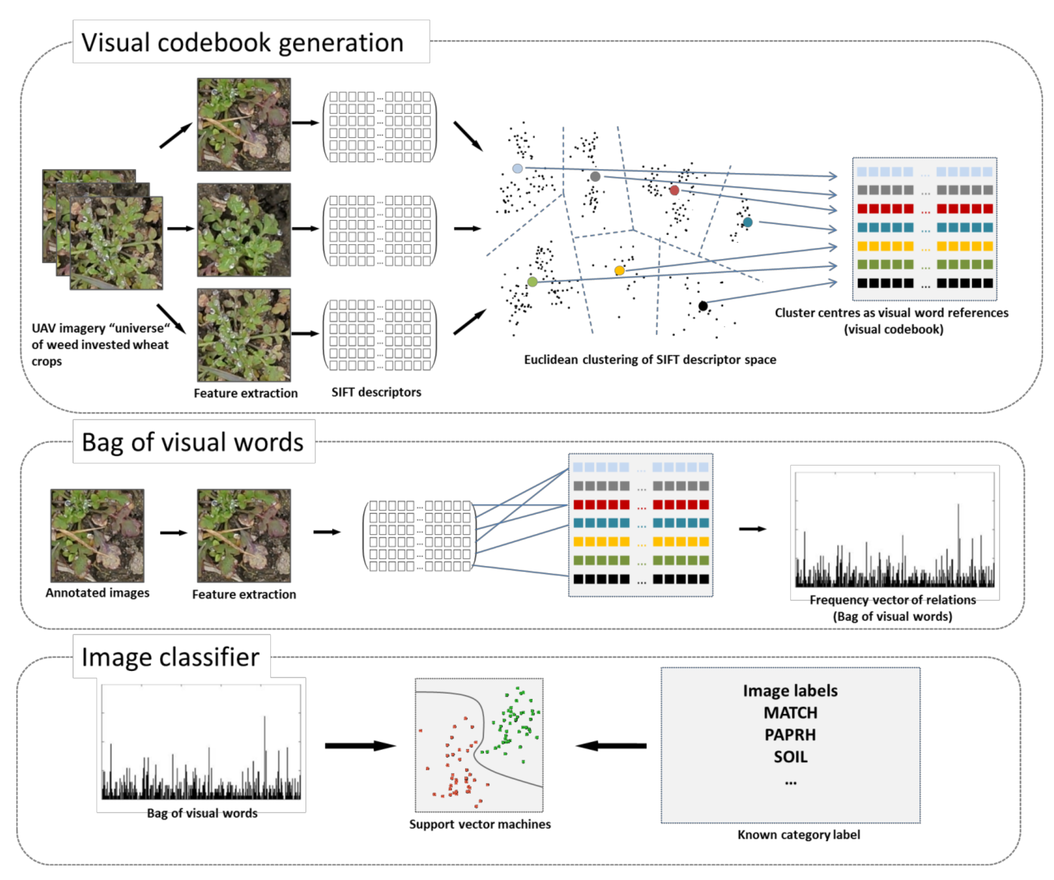
The image classifier was generated with the BoVW concept, as given in Figure 4. The idea was to breakdown the content of an image in relation to a generalized set of features that was a priori derived from a large set of images. The generalized set of features or code words was referred to as the visual dictionary. The relations between the features of an image to this visual dictionary can be expressed as a frequency vector counting the numbers of unique relations between image features and code words (generalized features of the visual dictionary). This frequency vector is called the “bag of visual words” [47]. Combined with known labels of the images, these frequency vectors are then used for calibrating the image classifier.
We used only the sub-images (Figure 3) extracted from the UAS images located in the training area for calibrating (Figure 2). The sub-images were processed in three different color spaces before presenting them to the model for comparison, i.e., unprocessed RGB, a plain gray-scale transformation using the Matlab built-in function rgb2gray, and a transformation to HSV color space by rgb2hsv, which applies the algorithm of Smith [48].
The visual dictionaries were built by a modified framework, originating from the computer vision feature library (VLFEAT, Version 0.9.21) of Matlab [49]. As a standard algorithm for key point detection and description, this toolbox uses a blob detector based on SIFT [50]. To find out the optimal descriptor scale, spatial histograms were calculated for different bins, which varied by pixel widths of 2, 4, and 8. The visual dictionary was built using K-means clustering. This meant that the code words, which constitute the visual dictionary, represented the average Euclidean center of key point descriptors mapped to one of n clusters that were found by the average Euclidean dissimilarity from cluster to cluster. This mapping of new input data into one of the clusters by looking for the closest center was tested for vector quantization (VQ) and the k-dimensional binary tree (KDTREE). In contrast to the linear approximating process of VQ, KDTREE uses a hierarchal data structure to find nearest neighbors by partitioning the source data recursively along the dimension of the maximum variance [49].
The dictionary size, e.g., the number of code words (or cluster centers), were systematically varied from 200, 500, and 1000. Key point descriptors of the new images were related with an approximate nearest neighbor search to construct the BoVW vectors. Support vector machines were used to calibrate the image classifier with linear kernel and different solvers. While the Stochastic Dual Coordinate Ascent solver (SDCA) maximizes the dual SVM objective, the Stochastic Gradient Descent (SGD) minimizes the primal SVM objective. We also tested the open-source Large Linear Classification library (liblinear), which implements linear SVMs and logistic regression models using a coordinate descent algorithm [51]. All hyper parameters of the BoVW framework were systematically permuted, which produced a number of n = 486 trained BoVW models in total (Table 3). All analyses were done using MATLAB (Version 2016b, The Mathworks, Natick, MA, USA).
2.4. Mapping the Models on the UAS Field Scenes
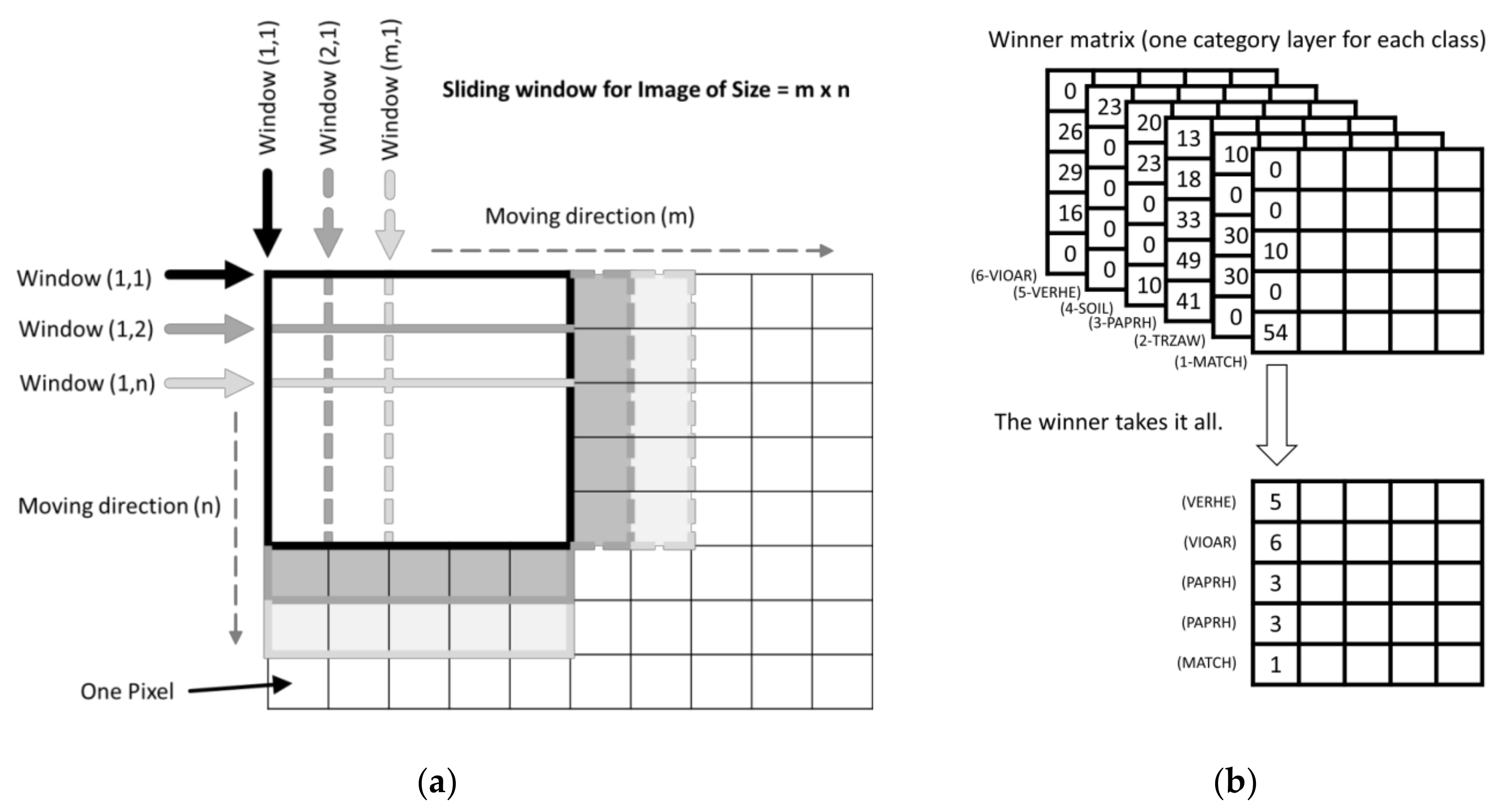
A sliding window approach (Figure 5a) was used for mapping the BoVW models, on a total of n = 34 UAS images of the test zone [52,53]. To accomplish this, the UAS images were segmented into numerous smaller sub-images with different block sizes (BS) of 50 and 200 px and overlaps (shift) of 5 and 20 px, respectively. The lower the value of the shift is, the higher the overlap of the sub-images and the finer the sampling rate. Then, the BoVW model was evaluated over all rectangular sub-images, and a value of 1 was added to each pixel position of BS in the corresponding category layer. Each image region was subsequently classified using the BoVW model, and its result was summarized in the corresponding layer. Finally, a quality function mapped the category number into a winner matrix considering the object’s location and the maximum value across the categories of layers (Figure 5b). The mapping results were validated by n = 8686 ground truthing points within the UAS field scenes from the test set area (see Figure 2).
2.5. Metrics for Evaluation
The testing of the BoVW models and the generated maps was done using the sub-images and the annotations made in the UAS images both taken from the test zone. The weed classification approach shown here considered not only a global crop–weed classification, but it discriminated between four different weed species, soil, and winter wheat. Nevertheless, this task of detection needs a metric to evaluate the quality of decisions. True Positive (TP), True Negative (TN), False Negative (FN), and False Positive (FP), were calculated from 6 × 6 confusion matrices for each class. For example, in case of MATCH, the correct predictions of the category MATCH are called TP, whilst TN is the sum of all other correct predictions of not MATCH categories. FP summarizes cases in which MATCH is falsely predicted as MATCH, whilst in reality it belongs to another category; whereas FN describes cases in which another category is falsely predicted as MATCH. TP, TN, FP, and FN were used to estimate the performance of the BoVW models with the following metrics:
Precision represents the predicted positives that are truly real positives (Equation (1)). That refers to how well a given model can deliver only correctly classified species in the result set. In contrast, recall (also known as sensitivity) is the probability of predicting positives being real positives (Equation (2)). It reflects how many plants, predicted in a specific category, are truly part of this category. The overall accuracy was calculated by Equation (3). All metrics calculations were done in R [54] using the ‘caret’ package [55].
3. Results
3.1. Image Classification
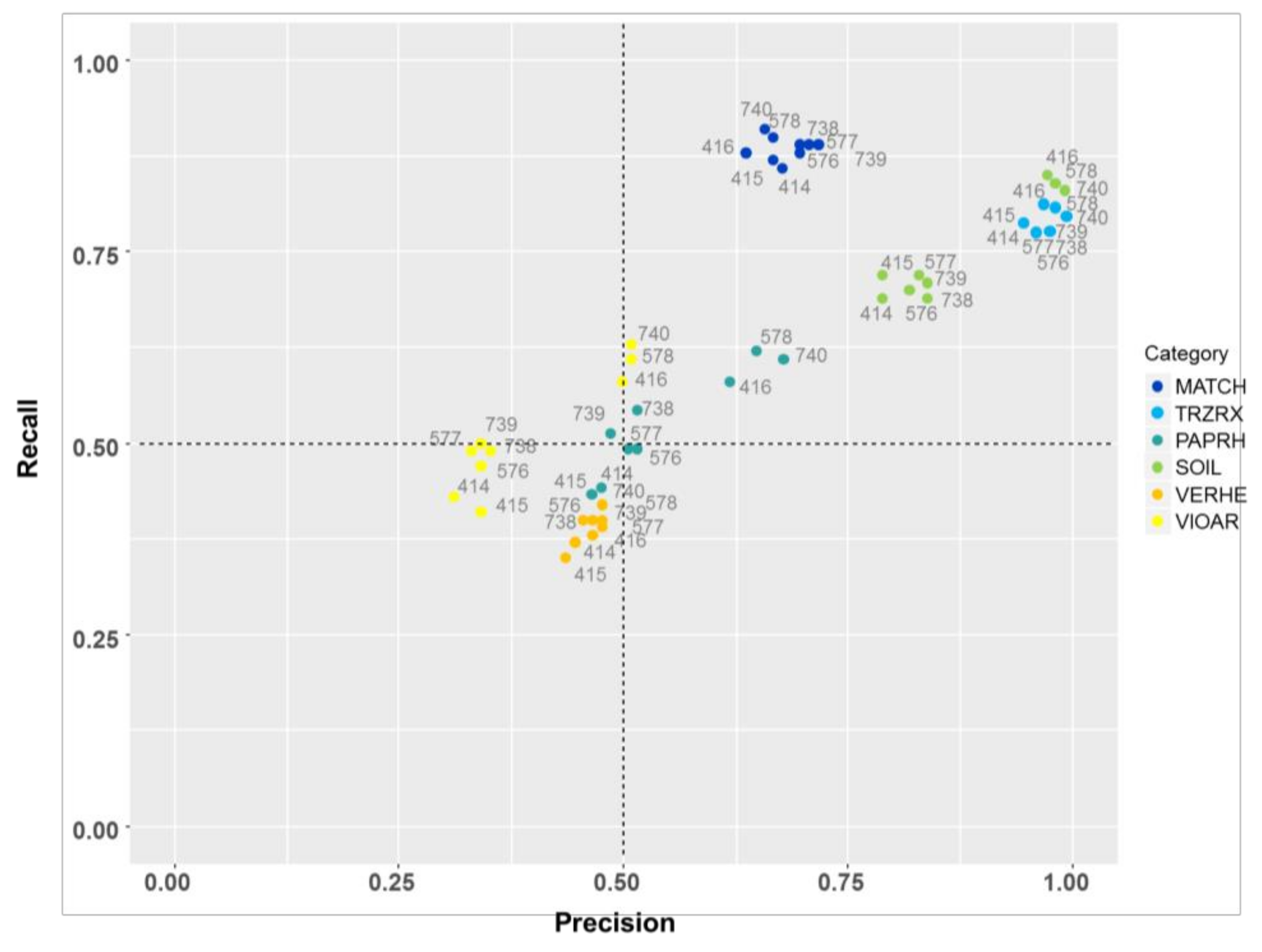
The classification results of the BoVW models with different vocabulary sizes of the visual codebook and transformations of the input images are summarized in Table 4. In short, only the results from the SDCA solver and KD-TREE quantization were shown here because results from LIBLINEAR and VQ did not provide better accuracies and computing performance was around two times slower (see Table S1). Generally, there was a slight increase of the overall classification accuracy when increasing the vocabulary size from 200 to 500, whereas the increase in accuracy from the 500 to 1000 vocabulary size was negligible. When transforming the images to HSV color space before subjecting them to the BoVW model, the overall classification accuracies were improved.
In more detail, the identification of soil and wheat images had a higher precision (>95%), in comparison to the identification of weed images (<70%). However, to some extent, there was the chance that weed images were falsely classified as soil or wheat, as can be seen by the recall reaching only 80–85% (Figure 6). Among the weed species, MATCH was most precisely identified in the test image set, whilst VERHE and VIOAR the had worst precision. This is corroborated by the confusion matrix of model 578 (Table 5, vocabulary size 500 and transformation HSV), which shows in more detail that VERHE and VIOAR had a high misclassification rate between each other. Obviously, the BoVW model confused both weed species because of its high similarity in visual appearance. However, the HSV transformation positively influenced the precision and recall of the VERHE and VIOAR models, as well as the identification of the soil background; whereas it had almost no effect or even an unfavorable effect on the MATCH and PAPRH models.
3.2. BoVW Mapping of the UAS Field Scenes
The BoVW models were used to predict categories continuously over the UAS field scenes to map the occurrences of soil, wheat, and weed species. We compared the model performances of two different window block sizes (50 and 200 px) and two step sizes (5 and 20 px) of the sliding window computing (Table 5 and Table 6 and Table S2). Generally, with finer filtering and scanning, the overall accuracy increased about 20% for the pixel-exact validation. The precision of the individual categories showed a similar pattern as the models of the image test set. Soil and wheat were identified with the highest precision, greater than 90%, for the models with finer filtering. This showed that generally a good differentiation between wheat, background, and weeds was possible using the mapping approach. However, whilst the soil category had a high precision for both fine and coarse filtering, the recall for soil in the case of coarse filtering was quite low. This meant that a lot of wheat and weed images were wrongly classified into the soil category. According to the confusion matrices shown in Table 5 and Table 6, this was particularly the case for VERHE and VIOAR. Nevertheless, with finer filtering, the recall for SOIL strongly increased from 38 to 77%, whilst the rate of misclassifications of VERHE and VIOAR remained almost constant.
In terms of the four different altitudes of the unmanned aerial vehicles (UAV) platform, the overall accuracy increased with choosing a lower altitude for the UAV platform. This gradient was stronger with coarser filtering. However, it is noteworthy that in most cases, it was not the lowest altitude that yielded the best accuracy, but it was the altitude between 2.5 and 4.0 m. Amongst the weed categories, except for PAPRH, the precision increased with finer filtering. MATCH had the highest mapping precision with 87%, whilst the performance of the other weed species was mainly underwhelming, except at the lowest altitude, at which VIOAR and PAPRH could obtain high precision values. However, with increasing altitude, the mapping precision of VIOAR and PAPRH strongly decreased and was far below 50%.
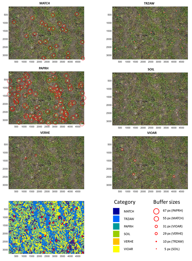
It is rather hard to match the ground truthing location exactly with one pixel, because of its small dimensions in reality. When allowing a small tolerance as a buffer around the prediction location that corresponds to the average plant dimensions, the overall accuracy strongly increased (Table 7) and was greater than 90% for all altitudes of the finer filtering (Table 8), with the highest accuracy at altitudes between 2.5–4.0 m (compare Table 9 and Table 10). This meant that the models predicted well, the right category in the immediate neighborhood of the ground truthing location. This was further supported by the prediction maps given in Figure 7 and Figure S3, for one of the UAS images. It can be seen quite strikingly, that the category soil shines through the plants similar to a background matrix, whereas the wheat plants assembled regular, long stripes within the map because of the seed rows. The different weed species, however, were spatially irregularly located in between the wheat rows. The white markings of the maps signified the ground truthing location of the predicted categories, and the red circles delineated the tolerance buffers allowed around the prediction points. In almost all cases, the correct category lay within the tolerance buffer and showed the high validity of the map.
4. Discussion
The BoVW model proposed in this study was able to differentiate weeds from crops in the cluttered UAS imagery with similar accuracy (>90%), compared to research studies using OBIA, supervised classification, or image recognition, for weed classification. For example, Peña et al. [42] could generate weed–crop maps from UAS imagery using an OBIA approach with an 86% overall accuracy for discriminating three categories of weed coverage in maize crops. Huang et al. [45] were able to differentiate rice from unspecified weeds using a patch based convolutional neural network, with an accuracy of 97%. However, our study focused on differentiating various weed species from winter wheat. Most similar to our study would be the study of Dyrmann et al. [41], when solely focusing on the image set alone. For wheat (Triticum aestivum), MATCH, PAPRH, VERHE, and VIOAR obtained mixed classification accuracies with 92%, 90%, 69%, 45%, and 33%, respectively. In comparison, we achieved similar results with 98%, 66%, 65%, 48%, and 51%, respectively, for the same plant species. However, results cannot be directly compared with each other, because in their study they tested 21 plant species and images, which were recorded from a constant altitude, whereas in this study only 5 plant species were tested, but images were acquired from an unstable UAV platform with an altitude range between 1.0 and 6.0 m.
The use of UAS imagery for model calibration could also have influenced the accuracy of the BoVW model. However, we found it more logical to use a realistic image data set than to rely solely on a data set acquired under laboratory conditions where illumination, shading, image sharpness, and resolution were held constant. It might be interesting to improve the calibration data set with accurate image data acquired under controlled conditions. The altitude of the UAV platform had an influence on the mapping of VIOAR and VERHE, which might be explained by their small plant sizes. Since the BoVW model significantly depends on a unique collection of key point descriptor information, then with increasing altitude this information becomes increasingly homogeneous with other categories. Specifically, due to the high resemblance of VIOAR and VERHE, the distinctive form specific information might get lost in the descriptors with higher altitude, due to lower spatial resolution of the images. Still, VIOAR reached a 79% mapping accuracy when allowing a plant specific tolerance buffer.
It is difficult to match exactly the midpoint of the ground truthing locations because of the small dimensions of one pixel in reality. Allowing a small, plant-specific buffer was more realistic than the pixel-exact testing, because it integrated the classification results in its nearest vicinity and considered the multiple testing during the scanning process whilst mapping. The visual evaluation of the weed maps corroborated this approach. Furthermore, it might be discussed that the model calibration may have been influenced by the rather unbalanced distribution of the annotations. This was partly unavoidable owing to the general abundance of weeds in the UAS imagery. However, we had at least 1000 annotations in each category. Contrary to neural network approaches, we spared data augmentation because the SIFT features used were rotation and translation invariant. We also did not segment the images before presenting them to the model because we encountered in the cluttered UAS images dry old leaves, stones, or soil with different illumination due to micro relief, which might pose a problem for simple segmentation procedures, such as image thresholding. We argue that the implementation of a background category will give better results in the end, especially if more data will be integrated subsequently.
5. Conclusions
With high resolution UAS imagery, we were able to map weeds on a species level within a winter wheat field. For this research, we annotated a large set of images taken from a UAV platform at different altitudes, and calibrated bag of visual words models based on SIFT image features and support vector machine classification. The validation with an independent image set showed a producer’s accuracy of 98%, for differentiating wheat crops from images with weeds and images with soil background. Among the weed species, Matricaria recutita L. showed the highest classification accuracy, whereas for Viola arvensis M. and Veronica hederifolia L., the models were weaker and showed signs of confusing both species with each other. The choice of the hyper-parameters for the BoVW models had only little influence on the outcomes. The weed maps generated by the BoVW models were able to distinguish weeds from crops and single weed species, with an accuracy of nearly 90% or greater. Regarding this kind of mapping, high resolution images with the capability of resolving even subtle details of crop and weed plants are an important prerequisite. Therefore, scanning resolution and altitude had a strong effect on the mapping accuracy of the UAS images and generally the better resolution, the better the map quality. Relating to SSWM, our approach would enable the selection of the right herbicide based on the distribution of the weed species in the classified UAS images. Further research will be directed to improve the generalization capabilities of the models by enhancing the annotation database by implementing more image data from different crop–weed associations and regions.
Supplementary Materials
The following are available online at https://0-www-mdpi-com.brum.beds.ac.uk/2072-4292/10/10/1530/s1, Table S1: Precision and recall values of all the models tested with an independent image set. KDTREE and VQ were used as quantizer, and SDCA, SVM, and liblinear as solver; Table S2: Precision and recall values of all the models tested on UAS field images using the sliding window approach. Figure S3: Category map of the spatial distribution of weeds, winter wheat, and soil.
Author Contributions
Conceptualization, M.P., M.S., and H.N.; Methodology, M.S. and M.P.; Software, M.P.; Validation, M.P., M.S., and H.N.; Formal Analysis, M.P.; Investigation, M.P.; Resources, H.N.; Data Curation, M.S.; Writing—Original Draft Preparation, M.S., M.P., and H.N.; Writing—Review and Editing, H.N.; Visualization, M.P. and M.S.; Supervision, H.N.; Project Administration, H.N. and M.P.; Funding Acquisition, H.N.
Funding
This research received no external funding.
Acknowledgments
We thank the staff of the JKI for their technical assistance, specifically Annika Behme and Werner Löhr, for their precious assistance in annotating weeds and ground truthing in numerous field trials. We thank Dominik Feistkorn and Arno Littman for conducting the flight missions and we thank Prof. Dr. Peter Zwerger for having made possible our investigations at his institute.
Conflicts of Interest
The authors declare no conflicts of interest.
References
- Spitters, C.J.T.; Van Den Bergh, J.P. Competition between crop and weeds: A system approach. In Biology and Ecology of Weeds; Holzner, W., Numata, M., Eds.; Springer Netherlands: Dordrecht, The Netherlands, 1982; pp. 137–148. ISBN 978-90-481-8519-1. [Google Scholar] [Green Version]
- Zimdahl, R.L. Fundamentals of Weed Science, 3rd ed.; Elsevier/Academic Press: Amsterdam, The Netherlands; Boston, MA, USA, 2007; ISBN 978-0-12-372518-9. [Google Scholar]
- Munier-Jolain, N.M.; Guyot, S.H.M.; Colbach, N. A 3D model for light interception in heterogeneous crop:weed canopies: Model structure and evaluation. Ecol. Model. 2013, 250, 101–110. [Google Scholar] [CrossRef]
- Hume, L. Yield losses in wheat due to weed communities dominated by green foxtail [Setaria viridis (L.) Beauv.]: A multispecies approach. Can. J. Plant Sci. 1989, 69, 521–529. [Google Scholar] [CrossRef]
- Milberg, P.; Hallgren, E. Yield loss due to weeds in cereals and its large-scale variability in Sweden. Field Crops Res. 2004, 86, 199–209. [Google Scholar] [CrossRef]
- Fahad, S.; Hussain, S.; Chauhan, B.S.; Saud, S.; Wu, C.; Hassan, S.; Tanveer, M.; Jan, A.; Huang, J. Weed growth and crop yield loss in wheat as influenced by row spacing and weed emergence times. Crop Prot. 2015, 71, 101–108. [Google Scholar] [CrossRef]
- Food and Agriculture Organization of the United Nations. FAOSTAT Statistics Database; Food and Agriculture Organization of the United Nations: Rome, Italy, 2013. [Google Scholar]
- Kniss, A.R. Long-term trends in the intensity and relative toxicity of herbicide use. Nat. Commun. 2017, 8, 14865. [Google Scholar] [CrossRef] [PubMed] [Green Version]
- Rendon-von Osten, J.; Dzul-Caamal, R. Glyphosate residues in groundwater, drinking water and urine of subsistence farmers from intensive agriculture localities: A survey in Hopelchén, Campeche, Mexico. Int. J. Environ. Res. Public Health 2017, 14, 595. [Google Scholar] [CrossRef] [PubMed]
- Rose, M.T.; Cavagnaro, T.R.; Scanlan, C.A.; Rose, T.J.; Vancov, T.; Kimber, S.; Kennedy, I.R.; Kookana, R.S.; Zwieten, L.V. Impact of herbicides on soil biology and function. Adv. Agron. 2016, 136, 133–220. [Google Scholar]
- European Food Safety Authority. The 2015 European Union report on pesticide residues in food. EFSA J. 2017, 15. [Google Scholar] [CrossRef]
- Christensen, S.; Heisel, T.; Walter, A.M.; Graglia, E. A decision algorithm for patch spraying. Weed Res. 2003, 43, 276–284. [Google Scholar] [CrossRef]
- Christensen, S.; SøGaard, H.T.; Kudsk, P.; NøRremark, M.; Lund, I.; Nadimi, E.S.; JøRgensen, R. Site-specific weed control technologies. Weed Res. 2009, 49, 233–241. [Google Scholar] [CrossRef]
- Jensen, P.K. Target precision and biological efficacy of two nozzles used for precision weed control. Precis. Agric. 2015, 16, 705–717. [Google Scholar] [CrossRef]
- Lelong, C.C.D.; Burger, P.; Jubelin, G.; Roux, B.; Labbé, S.; Baret, F. Assessment of unmanned aerial vehicles imagery for quantitative monitoring of wheat crop in small plots. Sensors 2008, 8, 3557–3585. [Google Scholar] [CrossRef] [PubMed]
- Schmale, D.G.; Dingus, B.R.; Reinholtz, C. Development and application of an autonomous unmanned aerial vehicle for precise aerobiological sampling above agricultural fields. J. Field Robot. 2008, 25, 133–147. [Google Scholar] [CrossRef]
- Xiang, H.T.; Tian, L. An automated stand-alone in-field remote sensing system (SIRSS) for in-season crop monitoring. Comput. Electron. Agric. 2011, 78, 1–8. [Google Scholar] [CrossRef]
- Lebourgeois, V.; Begue, A.; Labbe, S.; Houles, M.; Martine, J.F. A light-weight multi-spectral aerial imaging system for nitrogen crop monitoring. Precis. Agric. 2012, 13, 525–541. [Google Scholar] [CrossRef]
- Rasmussen, J.; Nielsen, J.; Garcia-Ruiz, F.; Christensen, S.; Streibig, J.C. Potential uses of small unmanned aircraft systems (UAS) in weed research. Weed Res. 2013, 53, 242–248. [Google Scholar] [CrossRef]
- Pflanz, M.; Feistkorn, D.; Nordmeyer, H. Unkrauterkennung mit Hilfe unbemannter Luftfahrzeuge. Julius-Kühn-Arch. 2014, 443, 396–403. [Google Scholar]
- Marceau, D.J.; Hay, G.J. Remote sensing contributions to the scale issue. Can. J. Remote Sens. 1999, 25, 357–366. [Google Scholar] [CrossRef]
- Zhang, J.-H.; Ke, W.; Bailey, J.; Ren-Chao, W. Predicting nitrogen status of rice using multispectral data at canopy scale. Pedosphere 2006, 16, 108–117. [Google Scholar] [CrossRef]
- Rama Rao, N.; Garg, P.; Ghosh, S.; Dadhwal, V. Estimation of leaf total chlorophyll and nitrogen concentrations using hyperspectral satellite imagery. J. Agric. Sci. 2008, 146, 65–75. [Google Scholar] [CrossRef]
- Schirrmann, M.; Giebel, A.; Gleiniger, F.; Pflanz, M.; Lentschke, J.; Dammer, K.-H. Monitoring agronomic parameters of winter wheat crops with low-cost UAV imagery. Remote Sens. 2016, 8, 706. [Google Scholar] [CrossRef]
- Pflanz, M.; Nordmeyer, H. Automatisierte Unkrauterkennung auf dem Acker–Möglichkeiten und Grenzen. Julius-Kühn-Arch. 2016, 452, 241–248. [Google Scholar]
- Borregaard, T.; Nielsen, H.; Nørgaard, L.; Have, H. Crop–weed discrimination by line imaging spectroscopy. J. Agric. Eng. Res. 2000, 75, 389–400. [Google Scholar] [CrossRef]
- Rao, N.R.; Garg, P.; Ghosh, S. Development of an agricultural crops spectral library and classification of crops at cultivar level using hyperspectral data. Precis. Agric. 2007, 8, 173–185. [Google Scholar] [CrossRef]
- Vrindts, E.; De Baerdemaeker, J.; Ramon, H. Weed detection using canopy reflection. Precis. Agric. 2002, 3, 63–80. [Google Scholar] [CrossRef]
- López-Granados, F.; Peña-Barragán, J.M.; Jurado-Expósito, M.; Francisco-Fernández, M.; Cao, R.; Alonso-Betanzos, A.; Fontenla-Romero, O. Multispectral classification of grass weeds and wheat (Triticum durum) using linear and nonparametric functional discriminant analysis and neural networks: Multispectral classification of grass weeds in wheat. Weed Res. 2008, 48, 28–37. [Google Scholar] [CrossRef]
- Lamb, D.W.; Weedon, M.M.; Rew, L.J. Evaluating the accuracy of mapping weeds in seedling crops using airborne digital imaging: Avena spp. in seedling triticale. Weed Res. 1999, 39, 481–492. [Google Scholar] [CrossRef]
- Langner, H.R.; Bottger, H.; Schmidt, H. A special vegetation index for the weed detection in sensor based precision agriculture. Environ. Monit. Assess. 2006, 117, 505–518. [Google Scholar] [CrossRef] [PubMed]
- Franz, E.; Gebhardt, M.R.; Unklesbay, K.B. Shape description of completely visible and partially occluded leaves for identifying plants in digital image. Trans. ASABE 1991, 34, 673–681. [Google Scholar] [CrossRef]
- Woebbecke, D.M.; Meyer, G.E.; Von Bargen, K.; Mortensen, D.A. Shape features for identifying young weeds using image analysis. Trans. ASAE 1995, 38, 271–281. [Google Scholar] [CrossRef]
- Zulkifli, Z.; Saad, P.; Mohtar, I.A. Plant leaf identification using moment invariants & general regression neural network. In Proceedings of the 2011 11th International Conference on Hybrid Intelligent Systems (HIS), Melaka, Malaysia, 5–8 December 2011; pp. 430–435. [Google Scholar]
- Rumpf, T.; Römer, C.; Weis, M.; Sökefeld, M.; Gerhards, R.; Plümer, L. Sequential support vector machine classification for small-grain weed species discrimination with special regard to Cirsium arvense and Galium aparine. Comput. Electron. Agric. 2012, 80, 89–96. [Google Scholar] [CrossRef]
- Persson, M.; Åstrand, B. Classification of crops and weeds extracted by active shape models. Biosyst. Eng. 2008, 100, 484–497. [Google Scholar] [CrossRef]
- Pahikkala, T.; Kari, K.; Mattila, H.; Lepistö, A.; Teuhola, J.; Nevalainen, O.S.; Tyystjärvi, E. Classification of plant species from images of overlapping leaves. Comput. Electron. Agric. 2015, 118, 186–192. [Google Scholar] [CrossRef]
- Kazmi, W.; Garcia-Ruiz, F.J.; Nielsen, J.; Rasmussen, J.; Jørgen Andersen, H. Detecting creeping thistle in sugar beet fields using vegetation indices. Comput. Electron. Agric. 2015, 112, 10–19. [Google Scholar] [CrossRef] [Green Version]
- Suh, H.K.; Hofstee, J.W.; IJsselmuiden, J.; van Henten, E.J. Sugar beet and volunteer potato classification using Bag-of-Visual-Words model, Scale-Invariant Feature Transform, or Speeded Up Robust Feature descriptors and crop row information. Biosyst. Eng. 2018, 166, 210–226. [Google Scholar] [CrossRef]
- Krizhevsky, A.; Sutskever, I.; Hinton, G.E. Imagenet classification with deep convolutional neural networks. In Advances in Neural Information Processing Systems; MIT Press: Cambridge, MA, USA, 2012; pp. 1097–1105. [Google Scholar]
- Dyrmann, M.; Karstoft, H.; Midtiby, H.S. Plant species classification using deep convolutional neural network. Biosyst. Eng. 2016, 151, 72–80. [Google Scholar] [CrossRef]
- Peña, J.M.; Torres-Sánchez, J.; de Castro, A.I.; Kelly, M.; López-Granados, F. Weed mapping in early-season maize fields using object-based analysis of unmanned aerial vehicle (UAV) Images. PLoS ONE 2013, 8, e77151. [Google Scholar] [CrossRef] [PubMed]
- Tamouridou, A.A.; Alexandridis, T.K.; Pantazi, X.E.; Lagopodi, A.L.; Kashefi, J.; Moshou, D. Evaluation of UAV imagery for mapping Silybum marianum weed patches. Int. J. Remote Sens. 2016, 1–14. [Google Scholar] [CrossRef]
- Hung, C.; Xu, Z.; Sukkarieh, S. Feature learning based approach for weed classification using high resolution aerial images from a digital camera mounted on a UAV. Remote Sens. 2014, 6, 12037–12054. [Google Scholar] [CrossRef]
- Huang, H.; Deng, J.; Lan, Y.; Yang, A.; Deng, X.; Zhang, L. A fully convolutional network for weed mapping of unmanned aerial vehicle (UAV) imagery. PLoS ONE 2018, 13, e0196302. [Google Scholar] [CrossRef] [PubMed]
- Brisset, P.; Drouin, A.; Gorraz, M.; Huard, P.-S.; Tyler, J. The paparazzi solution. In Proceedings of the 2nd US-European Competition and Workshop on Micro Air Vehicles, MAV, Sandestin, MA, USA, October 2006. [Google Scholar]
- Csurka, G.; Dance, C.R.; Fan, L.; Willamowski, J.; Bray, C. Visual Categorization with Bags of Keypoints. In Proceedings of the Workshop on Statistical Learning in Computer Vision, Prague, Czech Republic, 11–14 May 2004. [Google Scholar]
- Smith, A.R. Color gamut transform pairs. ACM Siggr. Comput. Graph. 1978, 12, 12–19. [Google Scholar] [CrossRef]
- Vedaldi, A.; Fulkerson, B. VLFeat: An open and portable library of computer vision algorithms. In Proceedings of the 18th ACM international conference on Multimedia, Firenze, Italy, 25–29 October 2010; pp. 1469–1472. [Google Scholar]
- Lowe, D.G. Distinctive image features from scale-invariant keypoints. Int. J. Comput. Vis. 2004, 60, 91–110. [Google Scholar] [CrossRef]
- Fan, R.-E.; Chang, K.-W.; Hsieh, C.-J.; Wang, X.-R.; Lin, C.-J. LIBLINEAR: A library for large linear classification. J. Mach. Learn. Res. 2008, 9, 1871–1874. [Google Scholar]
- Lampert, C.H.; Blaschko, M.B.; Hofmann, T. Beyond sliding windows: Object localization by efficient subwindow search. In Proceedings of the IEEE Conference on Computer Vision and Pattern Recognition, Anchorage, AK, USA, 23–28 June 2008; pp. 1–8. [Google Scholar]
- Forsyth, D.A.; Ponce, J. Computer Vision: A Modern Approach; Prentice Hall Professional Technical Reference: Englewood, NJ, USA, 2002; ISBN 0-13-085198-1. [Google Scholar]
- R Core Team. R: A Language and Environment for Statistical Computing; R Foundation for Statistical Computing: Vienna, Austria, 2017. [Google Scholar]
- Wing, M.K.C.J.; Weston, S.; Williams, A.; Keefer, C.; Engelhardt, A.; Cooper, T.; Mayer, Z.; Kenkel, B.; Team, R.C.; Benesty, M.; et al. Caret: Classification and Regression Training; Astrophysics Source Code Library: Houghton, MI, USA, 2017. [Google Scholar]
Figure 1.
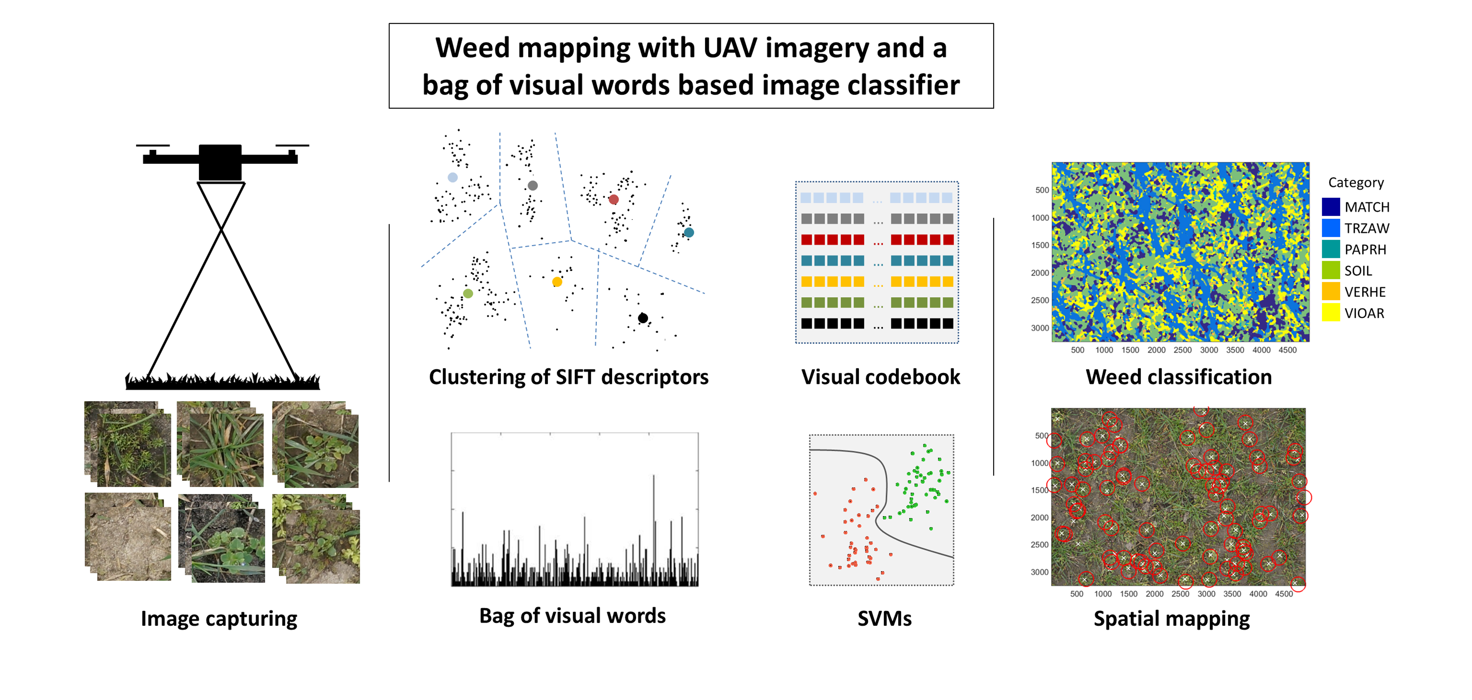
Capturing high resolution images at more than 100 waypoints (+) from Nadir. At a flight altitude of 5 m the ground sample distance (GSD) was 0.4 mm with a lens having a focal length of 60 mm and a camera equipped with an APS-C sensor.
Figure 1.
Capturing high resolution images at more than 100 waypoints (+) from Nadir. At a flight altitude of 5 m the ground sample distance (GSD) was 0.4 mm with a lens having a focal length of 60 mm and a camera equipped with an APS-C sensor.

Figure 2.
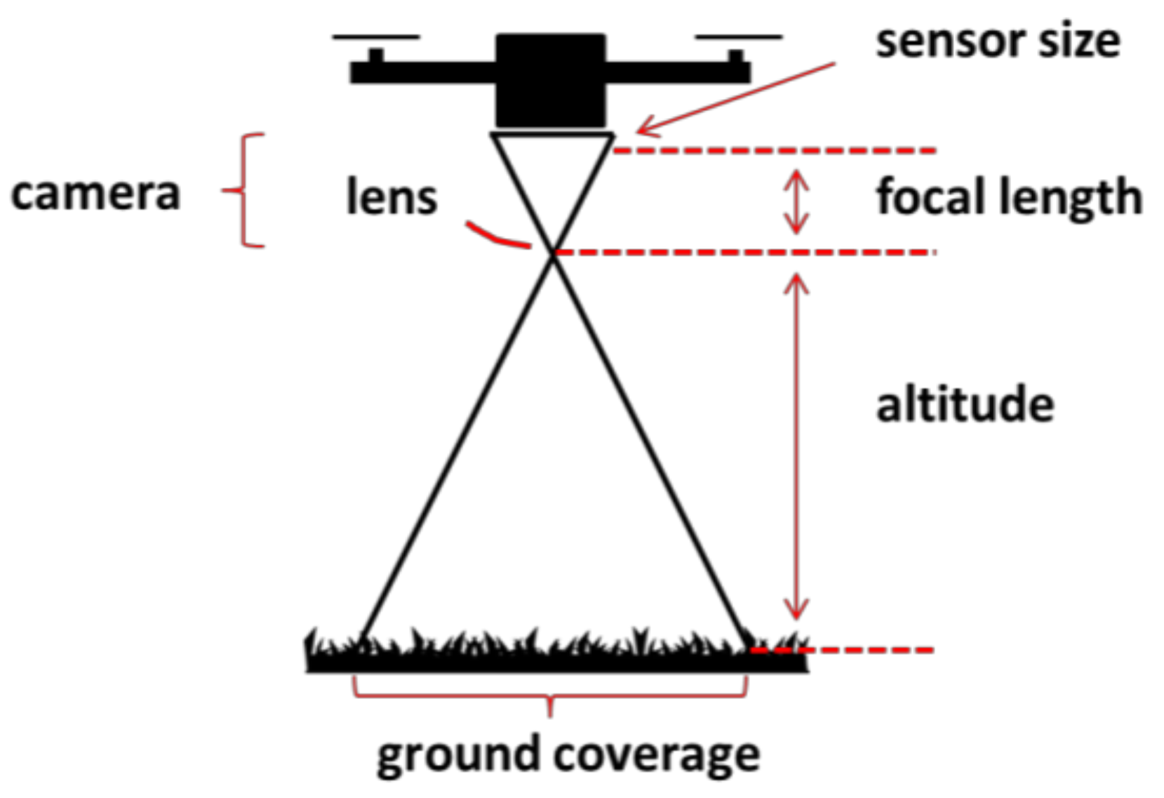
Test field of approx. 6.2 ha, unmanned aircraft system (UAS) flight routes (FL), image positions and allocation of images in test and training data sets. Coordinates shown are in UTM zone 32 N, ETRS89 (EPSG code: 5972).
Figure 2.
Test field of approx. 6.2 ha, unmanned aircraft system (UAS) flight routes (FL), image positions and allocation of images in test and training data sets. Coordinates shown are in UTM zone 32 N, ETRS89 (EPSG code: 5972).

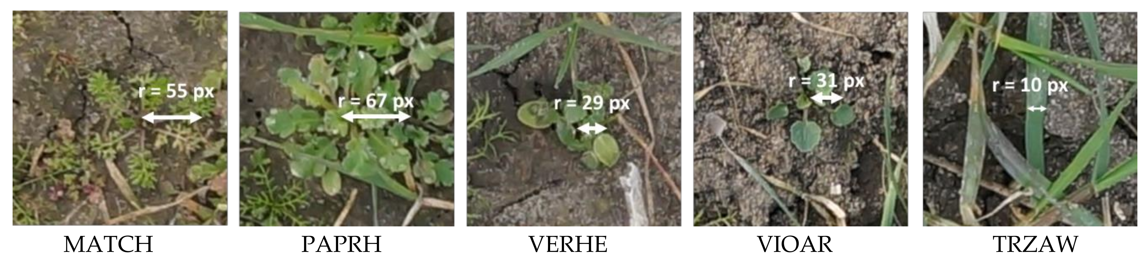
Figure 3.
Examples of sub-images extracted from the UAS imagery showing the different weed species and wheat plant. The average dimension (in pixel) was manually estimated.
Figure 3.
Examples of sub-images extracted from the UAS imagery showing the different weed species and wheat plant. The average dimension (in pixel) was manually estimated.

Figure 4.
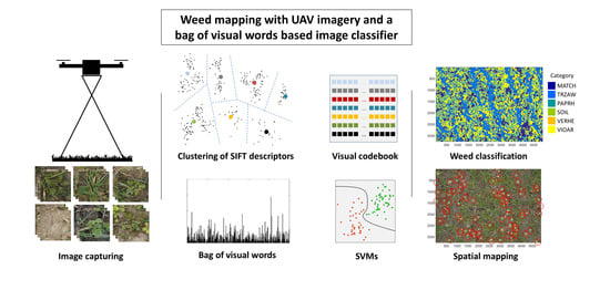
Bag of Visual Words (BoVW) framework: To train an image classifier using the BoVW concept, three steps need to be performed: First, a visual dictionary must be generated from many images. These images may be related to a specific theme, such as unspecific images from plants. From these images, the most relevant information will be extracted using key point extractors and descriptors. Depending on the type of the key point extractor, it finds key points at edges, corners, homogeneous regions, or blobs in the images, and the key point descriptor describes the immediate local neighborhood of the key points invariant to rotation or scale. The key point descriptions are collected over the entire image set and are generalized to a smaller set of code words by finding the centroids with a vector quantization method, such as k-means, to generate a visual dictionary. The second step involves a new labelled set of images. With the same key point descriptor as the visual dictionary that was built, the features of the new image will be extracted and described. The new key point descriptions are then referenced to the code words of the visual dictionary based on its similarity. The frequencies of the key point allocations are recorded over the code words to generate the BoVW vector. In the last step, the labelled BoVW vectors are used to train the image classifier using in our case a support vector machine (SVM). In case of a prediction given a new image, a new BoVW vector must be produced in relation to the codebook, and using the calibrated image classifier, the new BoVW vector will be decided to belong to a specific category, such as a specific weed species.
Figure 4.
Bag of Visual Words (BoVW) framework: To train an image classifier using the BoVW concept, three steps need to be performed: First, a visual dictionary must be generated from many images. These images may be related to a specific theme, such as unspecific images from plants. From these images, the most relevant information will be extracted using key point extractors and descriptors. Depending on the type of the key point extractor, it finds key points at edges, corners, homogeneous regions, or blobs in the images, and the key point descriptor describes the immediate local neighborhood of the key points invariant to rotation or scale. The key point descriptions are collected over the entire image set and are generalized to a smaller set of code words by finding the centroids with a vector quantization method, such as k-means, to generate a visual dictionary. The second step involves a new labelled set of images. With the same key point descriptor as the visual dictionary that was built, the features of the new image will be extracted and described. The new key point descriptions are then referenced to the code words of the visual dictionary based on its similarity. The frequencies of the key point allocations are recorded over the code words to generate the BoVW vector. In the last step, the labelled BoVW vectors are used to train the image classifier using in our case a support vector machine (SVM). In case of a prediction given a new image, a new BoVW vector must be produced in relation to the codebook, and using the calibrated image classifier, the new BoVW vector will be decided to belong to a specific category, such as a specific weed species.

Figure 5.
(a) Principle of the sliding window approach used; (b) One layer for each category was pre-allocated with the size m × n of the original image.
Figure 5.
(a) Principle of the sliding window approach used; (b) One layer for each category was pre-allocated with the size m × n of the original image.

Figure 6.
Precision-recall-plots of the different BoVW models shown in Table 4 for the classes (a) MATCH, (b) TRZAW, (c) PAPRH, (d) SOIL, (e) VERHE, and (f) VIOAR.
Figure 6.
Precision-recall-plots of the different BoVW models shown in Table 4 for the classes (a) MATCH, (b) TRZAW, (c) PAPRH, (d) SOIL, (e) VERHE, and (f) VIOAR.

Figure 7.
Weed classification results of the model 578 shown for the UAS image taken at field position 42. The sliding window has a block size of 50 px and a shift of 5 px. A category map (bottom left) draws the spatial distribution of weeds, winter wheat, and soil. Ground truthing points for MATCH (x), TRZAW (∆), and soil (□) illustrate the accuracies.


Table 1.
Summary of categories from weed species and crop plants, their EPPO-Codes, plant development stage, and specific plant dimensions. Category #4 comprises images from soil only and is not shown here.
Table 1.
Summary of categories from weed species and crop plants, their EPPO-Codes, plant development stage, and specific plant dimensions. Category #4 comprises images from soil only and is not shown here.
| Species | # | EPPO-Code | BBCH | Avg. Radius (px) |
|---|---|---|---|---|
| Matricaria recutita L. (Wild Chamomille) | 1 | MATCH | 16–18 | 55 |
| Papaver rhoeas L. (Common Poppy) | 3 | PAPRH | 17–19 | 67 |
| Veronica hederifolia L. (Ivyleaf Speedwell) | 5 | VERHE | 21 | 29 |
| Viola arvensis M. (Field Pansy) | 6 | VIOAR | 15 | 31 |
| Triticum aestivum L. (Winter Wheat) | 2 | TRZAW | 23 | 10 |
Table 2.
Allocation of annotated sub-images into train set and test set for wheat, soil, and the four weed species.
Table 2.
Allocation of annotated sub-images into train set and test set for wheat, soil, and the four weed species.
| n | MATCH | VERHE | PAPRH | VIOAR | TRZAW | SOIL | Total |
|---|---|---|---|---|---|---|---|
| Train Set | 6397 | 1728 | 1598 | 1701 | 2164 | 4077 | 17,665 |
| Test Set | 2086 | 891 | 711 | 1107 | 1038 | 1954 | 7787 |
| ∑ | 8483 | 2619 | 2309 | 2808 | 3202 | 6031 | 25,452 |
Table 3.
Permuted repetition of input parameters for generating n = 486 BoVW-models.
| Input | Variation |
|---|---|
| Vocabulary size | {200…500…1000} |
| Color space | {gray…rgb…hsv} |
| Number of spatial bins | {2…[2 4]…[2 4 8]} |
| Quantizer | {KDTREE…VQ} |
| SVM.C | {1…5…10} |
| SVM solver | {sdca… sgd…liblinear} |
Table 4.
Precision and recall values of the model testing with an independent image set. K-dimensional binary tree (KDTREE) was used as quantizer and Dual Coordinate Ascent solver (SDCA) as the support vector machines (SVM) solver.
Table 4.
Precision and recall values of the model testing with an independent image set. K-dimensional binary tree (KDTREE) was used as quantizer and Dual Coordinate Ascent solver (SDCA) as the support vector machines (SVM) solver.
| ID | Words | Color | Precision in % | Accuracy Overall in % | |||||
|---|---|---|---|---|---|---|---|---|---|
| MATCH | PAPRH | VERHE | VIOAR | TRZAW | SOIL | ||||
| 414 | 200 | gray | 67.16 | 47.12 | 44.56 | 31.71 | 95.28 | 79.43 | 64.53 |
| 415 | 200 | rgb | 66.35 | 45.85 | 44.33 | 34.60 | 94.99 | 79.38 | 64.53 |
| 416 | 200 | hsv | 63.14 | 61.74 | 47.14 | 49.59 | 97.21 | 97.44 | 72.40 |
| 576 | 500 | gray | 68.60 | 50.63 | 45.79 | 34.96 | 96.15 | 82.24 | 66.66 |
| 577 | 500 | rgb | 69.99 | 50.07 | 48.04 | 34.42 | 96.15 | 82.60 | 67.25 |
| 578 | 500 | hsv | 65.87 | 64.98 | 47.92 | 51.31 | 97.98 | 98.31 | 74.09 |
| 738 | 1000 | gray | 68.55 | 51.34 | 47.03 | 35.59 | 96.53 | 83.98 | 67.43 |
| 739 | 1000 | rgb | 71.28 | 48.24 | 47.92 | 35.32 | 96.63 | 83.57 | 67.86 |
| 740 | 1000 | hsv | 65.44 | 67.51 | 47.59 | 50.68 | 98.65 | 98.52 | 74.21 |
| Recall in % | |||||||||
| MATCH | PAPRH | VERHE | VIOAR | TRZAW | SOIL | ||||
| 414 | 200 | gray | 85.64 | 44.02 | 37.07 | 42.60 | 78.62 | 69.38 | 64.53 |
| 415 | 200 | rgb | 87.43 | 42.78 | 35.49 | 41.18 | 79.45 | 71.87 | 64.53 |
| 416 | 200 | hsv | 88.15 | 57.92 | 37.94 | 58.03 | 80.66 | 85.34 | 72.40 |
| 576 | 500 | gray | 87.52 | 49.18 | 39.92 | 46.80 | 78.34 | 69.96 | 66.66 |
| 577 | 500 | rgb | 88.65 | 49.24 | 38.77 | 48.78 | 78.27 | 71.51 | 67.25 |
| 578 | 500 | hsv | 90.28 | 61.68 | 41.78 | 60.62 | 80.71 | 83.63 | 74.09 |
| 738 | 1000 | gray | 88.65 | 54.15 | 40.33 | 48.88 | 78.22 | 69.12 | 67.43 |
| 739 | 1000 | rgb | 88.72 | 51.12 | 40.44 | 49.68 | 77.51 | 70.91 | 67.86 |
| 740 | 1000 | hsv | 91.18 | 60.76 | 42.27 | 62.75 | 79.75 | 83.01 | 74.21 |
Table 5.
Confusion matrix for the low resolution prediction (200/20) of model 578 on the UAS field scenes. The accuracy overall was 48%.
Table 5.
Confusion matrix for the low resolution prediction (200/20) of model 578 on the UAS field scenes. The accuracy overall was 48%.
| Actual/Predicted | 1 | 2 | 3 | 4 | 5 | 6 | Total | Recall | |
|---|---|---|---|---|---|---|---|---|---|
| 1 | MATCH | 921 | 50 | 52 | 11 | 323 | 1149 | 2506 | 79.06 |
| 2 | PAPRH | 51 | 309 | 8 | 5 | 103 | 235 | 711 | 77.44 |
| 3 | VERHE | 16 | 16 | 51 | 7 | 244 | 567 | 901 | 28.65 |
| 4 | VIOAR | 135 | 18 | 49 | 58 | 291 | 1025 | 1576 | 69.05 |
| 5 | TRZAW | 9 | 2 | 10 | 2 | 913 | 102 | 1038 | 48.18 |
| 6 | SOIL | 33 | 4 | 8 | 1 | 21 | 1887 | 1954 | 38.01 |
| Total | 1165 | 399 | 178 | 84 | 1895 | 4965 | 8686 | ||
| Precision | 36.75 | 43.46 | 5.66 | 3.68 | 87.96 | 96.57 | |||
Table 6.
Confusion matrix for the high resolution prediction (50/5) of model 578 on the UAS field scenes. The accuracy overall was 67%.
Table 6.
Confusion matrix for the high resolution prediction (50/5) of model 578 on the UAS field scenes. The accuracy overall was 67%.
| Actual/Predicted | 1 | 2 | 3 | 4 | 5 | 6 | Total | Recall | |
|---|---|---|---|---|---|---|---|---|---|
| 1 | MATCH | 2185 | 0 | 27 | 34 | 155 | 105 | 2506 | 68.47 |
| 2 | PAPRH | 281 | 89 | 35 | 113 | 112 | 81 | 711 | 71.20 |
| 3 | VERHE | 252 | 19 | 106 | 211 | 141 | 172 | 901 | 34.53 |
| 4 | VIOAR | 356 | 16 | 122 | 743 | 209 | 130 | 1576 | 66.10 |
| 5 | TRZAW | 17 | 1 | 16 | 16 | 936 | 52 | 1038 | 59.77 |
| 6 | SOIL | 100 | 0 | 1 | 7 | 13 | 1833 | 1954 | 77.24 |
| Total | 3191 | 125 | 307 | 1124 | 1566 | 2373 | 8686 | ||
| Precision | 87.19 | 12.52 | 11.76 | 47.14 | 90.17 | 93.81 | |||
Table 7.
Confusion matrix for the low resolution prediction (200/20) of model 578 on the UAS field scenes. When allowing a ground truthing tolerance considering plant dimensions, the accuracy overall was 80%.
Table 7.
Confusion matrix for the low resolution prediction (200/20) of model 578 on the UAS field scenes. When allowing a ground truthing tolerance considering plant dimensions, the accuracy overall was 80%.
| Actual/Predicted | 1 | 2 | 3 | 4 | 5 | 6 | Total | Recall | |
|---|---|---|---|---|---|---|---|---|---|
| 1 | MATCH | 1998 | 18 | 20 | 3 | 112 | 355 | 2506 | 94.47 |
| 2 | PAPRH | 16 | 560 | 4 | 0 | 43 | 88 | 711 | 96.05 |
| 3 | VERHE | 6 | 2 | 709 | 2 | 48 | 134 | 901 | 92.08 |
| 4 | VIOAR | 71 | 1 | 26 | 769 | 185 | 524 | 1576 | 99.23 |
| 5 | TRZAW | 2 | 0 | 5 | 0 | 980 | 51 | 1038 | 70.86 |
| 6 | SOIL | 22 | 2 | 6 | 1 | 15 | 1908 | 1954 | 62.35 |
| Total | 2115 | 583 | 770 | 775 | 1383 | 3060 | 8686 | ||
| Precision | 79.73 | 78.76 | 78.69 | 48.79 | 94.41 | 97.65 | |||
Table 8.
Confusion matrix for the high resolution prediction (50/5) of model 578 on the UAS field scenes. When allowing a ground truthing tolerance considering plant dimensions, the accuracy overall was 95%.
Table 8.
Confusion matrix for the high resolution prediction (50/5) of model 578 on the UAS field scenes. When allowing a ground truthing tolerance considering plant dimensions, the accuracy overall was 95%.
| Actual/Predicted | 1 | 2 | 3 | 4 | 5 | 6 | Total | Recall | |
|---|---|---|---|---|---|---|---|---|---|
| 1 | MATCH | 2478 | 0 | 2 | 0 | 18 | 8 | 2506 | 92.50 |
| 2 | PAPRH | 62 | 573 | 8 | 23 | 30 | 15 | 711 | 98.79 |
| 3 | VERHE | 14 | 2 | 864 | 11 | 3 | 7 | 901 | 95.47 |
| 4 | VIOAR | 94 | 5 | 29 | 1359 | 53 | 36 | 1576 | 97.42 |
| 5 | TRZAW | 1 | 0 | 2 | 1 | 1026 | 8 | 1038 | 90.48 |
| 6 | SOIL | 30 | 0 | 0 | 1 | 4 | 1919 | 1954 | 96.29 |
| Total | 2679 | 580 | 905 | 1395 | 1134 | 1993 | 8686 | ||
| Precision | 98.88 | 80.59 | 95.89 | 86.23 | 98.84 | 98.21 | |||
Table 9.
Correlation between precision, recall, altitude (ALT), and window filtering (block size, BS, and shift), where n is the number of ground truthing points from manual annotations of the images.
Table 9.
Correlation between precision, recall, altitude (ALT), and window filtering (block size, BS, and shift), where n is the number of ground truthing points from manual annotations of the images.
| ID | BS [px] | Shift [px] | ALT [m] | n | Precision in % | Accuracy Overall in % | |||||
|---|---|---|---|---|---|---|---|---|---|---|---|
| MATCH | PAPRH | VERHE | VIOAR | TRZAW | SOIL | ||||||
| 578 | 200 | 20 | 1.0–2.5 | 1177 | 58.55 | 89.08 | 0.00 | 24.14 | 93.84 | 97.77 | 73.24 |
| 578 | 200 | 20 | 2.5–4.0 | 1275 | 41.30 | 33.33 | 0.00 | 3.77 | 89.06 | 99.46 | 55.53 |
| 578 | 200 | 20 | 4.0–5.5 | 4144 | 37.39 | 28.87 | 2.88 | 0.83 | 89.46 | 93.14 | 40.15 |
| 578 | 200 | 20 | 5.5–6.0 | 2090 | 14.73 | 0.00 | 9.23 | 0.29 | 82.64 | 98.01 | 43.30 |
| 578 | 50 | 5 | 1.0–2.5 | 1177 | 83.22 | 13.79 | 0.00 | 87.93 | 82.88 | 86.59 | 73.15 |
| 578 | 50 | 5 | 2.5–4.0 | 1275 | 84.42 | 0.00 | 1.79 | 78.77 | 93.75 | 94.07 | 80.24 |
| 578 | 50 | 5 | 4.0–5.5 | 4144 | 88.40 | 12.26 | 10.86 | 37.87 | 94.09 | 93.59 | 63.88 |
| 578 | 50 | 5 | 5.5–6.0 | 2090 | 88.60 | 0.00 | 15.38 | 29.86 | 86.50 | 98.56 | 65.12 |
| Recall in % | |||||||||||
| MATCH | PAPRH | VERHE | VIOAR | TRZAW | SOIL | ||||||
| 578 | 200 | 20 | 1.0–2.5 | 1177 | 88.12 | 81.15 | 0.00 | 82.35 | 74.86 | 63.99 | 73.24 |
| 578 | 200 | 20 | 2.5–4.0 | 1275 | 92.44 | 10.00 | 0.00 | 57.14 | 64.53 | 45.78 | 55.53 |
| 578 | 200 | 20 | 4.0–5.5 | 4144 | 73.31 | 77.27 | 10.00 | 46.67 | 37.22 | 28.49 | 40.15 |
| 578 | 200 | 20 | 5.5–6.0 | 2090 | 78.48 | NA | 54.55 | 25.00 | 50.20 | 38.29 | 43.30 |
| 578 | 50 | 5 | 1.0–2.5 | 1177 | 73.55 | 92.31 | 0.00 | 67.40 | 60.80 | 84.47 | 73.15 |
| 578 | 50 | 5 | 2.5–4.0 | 1275 | 87.37 | 0.00 | 16.67 | 69.29 | 69.77 | 90.41 | 80.24 |
| 578 | 50 | 5 | 4.0–5.5 | 4144 | 65.57 | 76.47 | 22.52 | 66.67 | 53.90 | 72.43 | 63.88 |
| 578 | 50 | 5 | 5.5–6.0 | 2090 | 62.90 | 0.00 | 53.85 | 58.52 | 62.56 | 72.51 | 65.12 |
Table 10.
Correlation between precision, recall, altitude (ALT), and window filtering (block size, BS, and shift), with buffered accuracies (tolerance threshold was chosen according to the average plant size of each species).
Table 10.
Correlation between precision, recall, altitude (ALT), and window filtering (block size, BS, and shift), with buffered accuracies (tolerance threshold was chosen according to the average plant size of each species).
| ID | BS [px] | Shift [px] | ALT [m] | n | Precision | Accuracy Overall in % | |||||
|---|---|---|---|---|---|---|---|---|---|---|---|
| MATCH | PAPRH | VERHE | VIOAR | TRZAW | SOIL | ||||||
| 578 | 200 | 20 | 1.0–2.5 | 1177 | 92.11 | 99.43 | 85.71 | 100.00 | 98.63 | 100.00 | 97.45 |
| 578 | 200 | 20 | 2.5–4.0 | 1275 | 91.69 | 100.00 | 83.04 | 66.98 | 95.31 | 99.46 | 89.65 |
| 578 | 200 | 20 | 4.0–5.5 | 4144 | 77.44 | 71.89 | 67.73 | 35.15 | 94.34 | 94.93 | 71.79 |
| 578 | 200 | 20 | 5.5–6.0 | 2090 | 67.46 | 75.00 | 84.84 | 45.22 | 91.96 | 98.19 | 79.38 |
| 578 | 50 | 5 | 1.0–2.5 | 1177 | 98.68 | 87.36 | 95.24 | 100.00 | 99.32 | 97.21 | 96.77 |
| 578 | 50 | 5 | 2.5–4.0 | 1275 | 100.00 | 100.00 | 99.11 | 95.28 | 98.44 | 99.46 | 98.75 |
| 578 | 50 | 5 | 4.0–5.5 | 4144 | 98.42 | 78.11 | 93.61 | 84.14 | 99.23 | 97.32 | 92.45 |
| 578 | 50 | 5 | 5.5–6.0 | 2090 | 99.52 | 100.00 | 96.70 | 78.84 | 98.39 | 99.10 | 95.22 |
| Recall | |||||||||||
| MATCH | PAPRH | VERHE | VIOAR | TRZAW | SOIL | ||||||
| 578 | 200 | 20 | 1.0–2.5 | 1177 | 100.00 | 98.30 | 94.74 | 100.00 | 97.96 | 93.96 | 97.45 |
| 578 | 200 | 20 | 2.5–4.0 | 1275 | 98.06 | 100.00 | 98.94 | 98.61 | 86.73 | 79.70 | 89.65 |
| 578 | 200 | 20 | 4.0–5.5 | 4144 | 91.69 | 95.01 | 85.48 | 98.67 | 56.64 | 46.60 | 71.79 |
| 578 | 200 | 20 | 5.5–6.0 | 2090 | 95.95 | 100.00 | 94.38 | 100.00 | 75.86 | 64.08 | 79.38 |
| 578 | 50 | 5 | 1.0–2.5 | 1177 | 96.15 | 100.00 | 86.96 | 95.60 | 94.16 | 98.31 | 96.77 |
| 578 | 50 | 5 | 2.5–4.0 | 1275 | 99.23 | 75.00 | 98.23 | 99.02 | 96.92 | 99.46 | 98.75 |
| 578 | 50 | 5 | 4.0–5.5 | 4144 | 90.04 | 99.04 | 93.02 | 96.73 | 84.10 | 94.50 | 92.45 |
| 578 | 50 | 5 | 5.5–6.0 | 2090 | 92.49 | 66.67 | 96.92 | 99.27 | 93.87 | 95.15 | 95.22 |
© 2018 by the authors. Licensee MDPI, Basel, Switzerland. This article is an open access article distributed under the terms and conditions of the Creative Commons Attribution (CC BY) license (http://creativecommons.org/licenses/by/4.0/).
Share and Cite
MDPI and ACS Style
Pflanz, M.; Nordmeyer, H.; Schirrmann, M. Weed Mapping with UAS Imagery and a Bag of Visual Words Based Image Classifier. Remote Sens. 2018, 10, 1530. https://0-doi-org.brum.beds.ac.uk/10.3390/rs10101530
AMA Style
Pflanz M, Nordmeyer H, Schirrmann M. Weed Mapping with UAS Imagery and a Bag of Visual Words Based Image Classifier. Remote Sensing. 2018; 10(10):1530. https://0-doi-org.brum.beds.ac.uk/10.3390/rs10101530
Chicago/Turabian StylePflanz, Michael, Henning Nordmeyer, and Michael Schirrmann. 2018. "Weed Mapping with UAS Imagery and a Bag of Visual Words Based Image Classifier" Remote Sensing 10, no. 10: 1530. https://0-doi-org.brum.beds.ac.uk/10.3390/rs10101530
Note that from the first issue of 2016, this journal uses article numbers instead of page numbers. See further details here.