Sparsity-Based Spatiotemporal Fusion via Adaptive Multi-Band Constraints


1
Department of Applied Mathematics, College of Sciences, China Jiliang University, Hangzhou 310018, China
2
Department of Geography and Resource Management, The Chinese University of Hong Kong, Hong Kong, China
3
Institute of Future Cities, The Chinese University of Hong Kong, Hong Kong, China
*
Author to whom correspondence should be addressed.
Remote Sens. 2018, 10(10), 1646; https://0-doi-org.brum.beds.ac.uk/10.3390/rs10101646
Submission received: 31 August 2018
/
Revised: 3 October 2018
/
Accepted: 6 October 2018
/
Published: 16 October 2018
(This article belongs to the Section Remote Sensing Image Processing)
Abstract
:Remote sensing is an important means to monitor the dynamics of the earth surface. It is still challenging for single-sensor systems to provide spatially high resolution images with high revisit frequency because of the technological limitations. Spatiotemporal fusion is an effective approach to obtain remote sensing images high in both spatial and temporal resolutions. Though dictionary learning fusion methods appear to be promising for spatiotemporal fusion, they do not consider the structure similarity between spectral bands in the fusion task. To capitalize on the significance of this feature, a novel fusion model, named the adaptive multi-band constraints fusion model (AMCFM), is formulated to produce better fusion images in this paper. This model considers structure similarity between spectral bands and uses the edge information to improve the fusion results by adopting adaptive multi-band constraints. Moreover, to address the shortcomings of the norm which only considers the sparsity structure of dictionaries, our model uses the nuclear norm which balances sparsity and correlation by producing an appropriate coefficient in the reconstruction step. We perform experiments on real-life images to substantiate our conceptual augments. In the empirical study, the near-infrared (NIR), red and green bands of Landsat Enhanced Thematic Mapper Plus (ETM+) and Moderate Resolution Imaging Spectroradiometer (MODIS) are fused and the prediction accuracy is assessed by both metrics and visual effects. The experiments show that our proposed method performs better than state-of-the-art methods. It also sheds light on future research.
1. Introduction
Remote sensing satellites are important tools for the monitoring of processes such as vegetation and land cover changes on the earth surface [1,2,3]. Because of technological limitations in sensor designs [4], compromises have to be made between spatial and temporal resolutions. For example, Moderate Resolution Imaging Spectroradiometer (MODIS) can visit the earth once a day with 500-m spatial resolution. As a comparison, the spatial resolution of Landsat Enhanced Thematic Mapper Plus (ETM+) is 30 m, but its revisiting period is 16 days. Such a limitation restricts the application of remote sensing in problems that need images high in both spatial and temporal resolutions. Spatiotemporal reflectance fusion models [5] have thus been developed to fuse image data from different sensors to obtain high spatiotemporal resolution images.
The Spatial and Temporal Adaptive Reflectance Fusion Model (STARFM) [6] is a pioneering fusion model based on a weighting method. This model uses neighboring pixels to compute the center pixel at a point in time with a weighting function, and the weights are determined by spectral difference, temporal difference and location distance. Furthermore, Zhu et al. [7] proposed an Enhanced Spatial and Temporal Adaptive Reflectance Fusion Model (ESTARFM) based on a STARFM algorithm to predict the surface reflectance of heterogeneous landscapes. Another improved STARFM method is a Spatial Temporal Adaptive Algorithm for mapping Reflectance Change (STAARCH) [8], which is designed to detect disturbance and changes in reflectance by using Tasseled Cap transformations. However, performance of the weighting methods are constrained because linear combination smooths out the changing terrestrial contents.
Another type of reflectance fusion method, known as dictionary learning methods, has been proposed to overcome the shortcoming of the weighting methods. Dictionary-based methods that use certain known dictionaries, such as wavelets and shearlets, have been proved to be efficient in multisensor and multiresolution image fusion [9,10,11]. In remote sensing data analysis, Moigne et al. [12] and Czaja et al. [13] proposed remote sensing image fusion methods based on wavelets and wavelet packet, respectively. Shearlet transform is also used in a fusion algorithm in [14] because shearlets can share the same optimality properties and enjoy similar geometrical properties. Using the capability of dictionary learning and sparsity-based methods in the super resolution analysis, Huang et al. [15] proposed a Sparse-representation-based Spatiotemporal Reflectance Fusion Model (SPSTFM) to integrate sparse representation and reflectance fusion by establishing correspondences between structures in high resolution images and their corresponding low resolution images through dictionary pair and sparse coding. SPSTFM assumes that high and low resolution images of the same area have the same sparse coefficients. Such assumption is, however, too restrictive [16]. Based on this idea, Wu et al. [17] proposed the Error-Bound-regularized Semi-Coupled Dictionary Learning (EBSCDL) model which assumes that the representation coefficients of the image pair have a stable mapping and coefficients of the dictionary pair have perturbations in the reconstruction step. Attempts have been made to improve the performance of the SCDL based models. For examples, Block Sparse Bayesian Learning for Semi-Coupled Dictionary Learning (BSBL-SCDL) [18] employs the structural sparsity of the sparse coefficients as a priori knowledge and Compressed Sensing for Spatiotemporal Fusion (CSSF) [19] considers explicitly the down-sampling process within the framework of compressed sensing for reconstruction. In comparison with the weighting methods, the advantage of the dictionary-learning-based methods is that they retrieve the hidden relationship between image pairs from the sparse coding space to better capture structure changes.
Besides the aforementioned methods, some researchers employed other approaches to fuse multi-source data. Unmixing techniques have been suggested for spatiotemporal fusion because of their ability to reconstruct images with high spectral fidelity [20,21,22,23,24]. Considering the mixed-class spectra within a coarse pixel, Xu et al. [25] proposed the Class Regularized Spatial Unmixing (CRSU) model. This method is based on the conventional spatial unmixing technique but is modified to include prior class spectra estimated by the known image pairs. To provide a formal statistical framework for fusion, Xue et al. [26] proposed Spatiotemporal Bayesian Data Fusion (STBDF) that makes use of the joint distribution to capture implicitly the temporal changes of images for the estimation of the high resolution image at a target point in time.
Considering structure similarity in spectral bands, structure information has been employed in pan-sharpening and image fusion. Shi et al. [27], for example, proposed a learning interpolation method for pan-sharpening by expanding sketch information of the high-resolution panchromatic (PAN) image which contains the structure features of the PAN image. Glasner et al. [28] verified that many structures in a natural image are similar at the same and different scales. Inspired by this, a self-learning approach was proposed by Khateri et al. [29] which uses similar structures at different levels to pan-sharpen the low resolution multi-spectral images. In multi-modality image fusion, Zhu et al. [30] proposed a method which decomposes images into cartoon and texture components, and preserves the structure information of two components based on spatial-based method and sparse representation, respectively.
However, none of these spatiotemporal fusion methods consider the structure similarity between spectral bands in the fusion procedure. Although different bands have different reflectance ranges, the edge information is still similar [31]. Obviously, a reconstruction model can have a better performance if such information can be effectively used to predict the unknown high resolution image. Otherwise, the dictionary pair obtained by the training image pair are inefficient to predict the unknown images because of the lack of information for the target time. This can be explained from the experience in machine learning in which the norm is too restrictive in encoding the unknown data in the prediction process because it only uses the sparsity structure of the dictionary [32,33]. Therefore, the reconstruction model needs a replacement of the norm to reduce the impact of insufficient information and to improve the representation ability of the dictionary pair.
We propose a new model in this paper to enhance spatiotemporal fusion performance. Our model uses the edge information in different bands via adaptive multi-band constraints to improve the reconstruction performance. To overcome the disadvantage of the norm, the nuclear norm is adopted as the regularization term to increase the efficiency of the learnt dictionary pair. Nuclear norm considers not only the sparsity but also the coordination in producing a suitable coefficient that can harmonize the sparse and collaborative representations adaptively [32,33].
Overall, the main contributions of this work can be summarized as follows.
- The multi-band constraints are employed to reinforce the structure similarity of different bands in spatiotemporal fusion.
- Considering the different structure similarity between two bands, the adaptive regularization parameters are proposed to determine the importance of each multi-band constraint adaptively.
- The nuclear norm is employed to replace the norm in the reconstruction model because the nuclear norm considers both sparsity and correlation of the dictionaries and can overcome the disadvantage of the norm.
The remainder of this paper is organized as follows. Our method for spatiotemporal fusion, called adaptive multi-band constraints fusion model (AMCFM), is proposed in Section 2. Section 3 discusses the experiments carried out to assess the effectiveness of the AMCFM and four state-of-the-art methods in terms of statistics and visual effects. We then conclude the paper with a summary and direction for future research in Section 4.
2. Methodology
2.1. Problem Definition
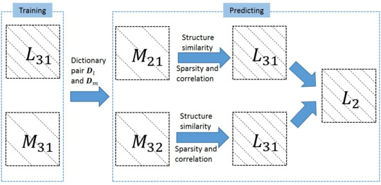
In the following, MODIS images are selected as low resolution images and Landsat ETM+ images are selected as high resolution images. As shown in Figure 1, our spatiotemporal fusion model requires three low resolution images , and , and two high resolution images and . The high resolution image is the target image that we want to predict. Let () and () be the high and low resolution difference images between and (), respectively. We assume that changes of remote sensing images between two points in time are linear. For effectiveness, the dictionary pair and is trained by the difference image pair and [15]. Then, the high resolution difference image can be produced by using the dictionary pair to encode the corresponding low resolution difference image . can be obtained in the same way. Finally, the high resolution image at time can be predicted as follows:
The weights and we used are same as those in [19], which take the average of the two predicted difference images.
2.2. Dictionary Learning Fusion Model
As mentioned above, the conventional dictionary learning fusion models are usually comprised of two steps: the dictionary pair training step and the reconstruction step. The whole process is performed on each band separately. Here, we show the mathematical formulation of these two steps in SPSTFM [15], which is the initial dictionary learning model.
- Dictionary pair training step:In the training step, the difference image pair, and , is used to train the high resolution dictionary and the corresponding low resolution dictionary as follows:where and are the column combination of the lexicographically stacked image patches, sampled randomly from and , respectively. is the column combination of the representation coefficients corresponding to every column in and , and is the regularization parameter. We adopt the K-SVD (K is the abbreviation for K-means and SVD is the abbreviation for Singular Value Decomposition) lgorithm [34] to solve for and in Equation (2).
- Reconstruction step:Then, is used to encode each patch of and the sparse coding coefficient is obtained by solving the optimization problem:where is a patch of . The corresponding patch of the high resolution image can be produced byThen, all patches of are merged to get the high resolution image . can be obtained in the same way and the target image can be predicted through Equation (1).
2.3. Adaptive Multi-Band Constraints Fusion Model
Our model uses the same strategy for dictionary pair training and focuses on the improvement of the reconstruction step. We propose the following model for spatiotemporal fusion by replacing the norm with the nuclear norm and incorporating the multi-band constraints. The reconstruction formulation is given as follows:
where , , and are the regularization parameters. is the nuclear norm of M that is the sum of all the singular values of matrix M. For a vector , represents a diagonal matrix whose diagonal elements are the corresponding elements of the vector . S is a high-pass detector filter. Here, we choose the two-dimensional Laplacian operator. The subscripts N, R and G mean the near-infrared (NIR), red and green band, respectively.
The dictionary pair and is trained by the difference images and which do not contain sufficient information of the images at time . When reconstructing or , if the model only uses the norm regularization, then the performance are unsatisfactory. It is more reasonable to integrate sparsity and correlation of the dictionaries. The nuclear norm term is just the kind of regularization that can adaptively balance sparsity and correlation via a suitable coefficient. As the property shown in [33,35],
where all columns of have unit norm. When the column vectors of are orthogonal, is equal to . When the column vectors of are highly correlated, will be close to [35]. Generally, remote sensing images in the dictionary are neither too independent nor too correlated because the test images and training images can contain high correlative information (i.e., stable land-cover) and independent information (i.e., land-cover change). Therefore, as shown in Equation (6), our model can benefit from both the norm and the norm. The advantage of the nuclear norm is that the nuclear norm can capture the correlation structure of the training images which the norm cannot.
The last three terms in the model are the multi-band regularization terms. Taking the NIR band as an example, denotes a high resolution patch of the NIR band and stands for the edge in the patch. These terms make the sparse codes (The codes may not be sparse based on the nuclear norm regularization, but, for convenience and without confusion, we still call them sparse codes.) in different bands no longer independent and reinforce the structure similarity of different bands.
Nevertheless, the nuclear norm regularization and multi-band regularization make it more complicated to solve the model. In Section 2.5, we propose the method to get a solution efficiently.
2.4. Adaptive Parameters between Bands
The ranges of reflectance in different bands are different in remote sensing images. In natural images, the range of the three channels is . Table 1 implicitly shows the range differences of three bands in terms of mean and standard deviation. Obviously, the structures are more similar when the means and standard deviations are closer. Based on this rationale, we propose an adaptive regularization parameter as follows:
where is the mean value of band c and is the standard deviation of band c; is a parameter to control the magnitude; and and can be obtained by the definition as well.
This parameter estimates the distribution of the reflectance values between two bands and produces a suitable parameter adaptively. When two bands have similar reflectance values, the parameter is close to . When the difference between two bands increases, the parameter decreases exponentially. The more similar two bands are, the more important a role the corresponding term plays in the model. This property fits such intuitive perception.
2.5. Optimization of the AMCFM
In this section, we solve the reconstruction model. For the optimization, a simplification is made first. We introduce the following vectors and matrices:
where and are concatenations of the sparse coefficients and low resolution image patches, respectively. is a dictionary that contains low resolution dictionaries of three bands in its diagonals. We also define as:
Then, Equation (5) can be simplified as follows:
Here, we use the alternating direction method of multipliers (ADMM) [36,37,38] algorithm to approximate the optimal solution of Equation (9). The optimization problem can be written as follows:
where is the dual variable in the ADMM algorithm. The augmented Lagrangian function of the optimization problem is given as
where is a positive scalar and is a scaled variable. The ADMM consists of the following iterations:
To minimize the augmented Lagrangian function, we solve each of the subproblems in Equation (12) by fixing the other two variables alternatively. For the step of updating , can be deduced as follows:
where . For a matrix , represents a vector whose ith element is the ith diagonal element of the matrix .
For the step of updating , can be calculated by the singular value thresholding operator [39] as follows:
where is the singular value shrinkage operator, which is defined as follows:
where is a positive scalar, is the singular value decomposition of a matrix , is the ith positive singular value of , and Now, we use to denote the singular value decomposition of and use to denote the ith positive singular value of . Then,
The implementation details of the whole reconstruction procedure based on the ADMM algorithm can be summarized in Algorithm 1.
| Algorithm 1 Reconstruction Procedure of the Proposed Method |
|
2.6. Strategy for More Bands
The proposed method considers the structure similarity of different bands and uses pairwise comparisons of the NIR, red and green bands. It should be noted that the relationship between n and m is quadratic (), where n and m represent the number of bands and the number of multi-band regularization terms, respectively. When n increases, the model will be much more complicated and difficult to solve.
Table 2 shows that adjacent bands have consistent bandwidths. This property indicates that structures of adjacent bands are more similar than those of the other pairs. It is thus reasonable to use adjacent bands constraints instead of pairwise comparisons of all bands. Otherwise, the number of combinations of the adjacent bands will get to be smaller and m will become linear to n (). Therefore, to efficiently extend it to more bands, we use the strategy that only considers structure similarity of two adjacent bands. This smaller model (AMCFM-s) can be reformulated as follows:
The procedure of solving AMCFM-s is the same as that of AMCFM. Details can be found in Section 2.5.
3. Experiments
The performance of our proposed method is compared to those of the four state-of-the-art methods for evaluation. ESTARFM [7] is a weighting method and CRSU [25] is an unmixing-based method. The other two are dictionary learning methods, named SPSTFM [15] and EBSCDL [17].
All programs are run in Windows 10 system (Microsoft, Redmond, Washington, DC, USA) and the processor is Intel Core i7-6700 3.40 GHz (Intel, Santa Clara, CA, USA). All of these fusion algorithms are coded in Matlab 2015a (MathWorks, Natick, MA, USA) except the ESTARFM, which is in IDL 8.5 (Harris Geospatial Solutions, Broomfield, CO, USA).
3.1. Experimental Scheme
In this experiment, we use the data acquired from the Boreal Ecosystem-Atmosphere Study (BOREAS) southern study area on 24 May, 11 July and 12 August in 2001, respectively. The products from Landsat ETM+ and MODIS (MOD09GHK) are selected as the source data for fusion. The Landsat image on 11 July 2001 is set as the target image for prediction. All the data are registered for fine geographic calibration.
In the fusion process, we focus on three bands: NIR, red and green. The size of the test images is 300 × 300. Before the test, we up-sample the MODIS images to the same resolution as the Landsat images via bi-linear interpolation because the spatial resolutions of these two source images are different.
3.2. Parameter Settings and Normalization
The parameters of AMCFM are set as follows. The dictionary size is 256, the patch size is 7 × 7, the overlap of patches is 4, the number of training patches is 2000, is 0.15, is 0, and are both 0, and is 0.1. All the comparative methods keep their original parameter settings.
Normalization can speed up the computation time and has an effect on the fusion results. As a preprocessing step, the high and low resolution images are normalized as follows:
where is the mean value of image and is the standard deviation of image .
3.3. Quality Measurement of the Fusion Results
Several metrics have been used to evaluate the fusion results by different methods. These metrics can be classified into two types, namely the band quality metrics and the global quality metrics.
We employ three assessment metrics, namely the root mean square error (RMSE), average absolute difference (AAD) and correlation coefficient (CC) to assess the performance of the algorithms in each band. The ideal result is 0 for RMSE and AAD, while it is 1 for CC.
Three other metrics are adopted to evaluate the global performance, including relative average spectral error (RASE) [40], Erreur Relative Globale Adimensionnelle de Synthèse (ERGAS) [41] and Q4 [42]. The mean RMSE (mRMSE) of three bands is also used as a global index. The ideal result is 0 for mRMSE, RASE and ERGAS, while it is 1 for Q4. It should be noted that Q4 is defined for four spectral bands. For our comparisons, the real part of a quaternion is set to 0.
3.4. Results
Table 3, Table 4 and Table 5 show the digital values of these methods in each band. All these methods can reconstruct the target high resolution image. ESTARFM has a good performance in the red band. CRSU performs well in the red band and green band of image 2, but, in most cases, this method has undesirable results. SPSTFM and EBSCDL have similar results and EBSCDL produces slightly higher quality in these three images. AMCFM and AMCFM-s produce the best results for NIR band. Moreover, AMCFM has the best or the second best results in almost all metrics, showing the stability and efficiency in its performance.
The global metrics of different methods are shown in Table 6, Table 7 and Table 8. AMCFM has the best global performance in all three images, except for Q4 in image 2 and ERGAS in image 3. Image 1 is best captured by our proposed model with a noticeable performance in all four metrics. The outstanding performance of AMCFM is attributed to its improved performance in the NIR band.
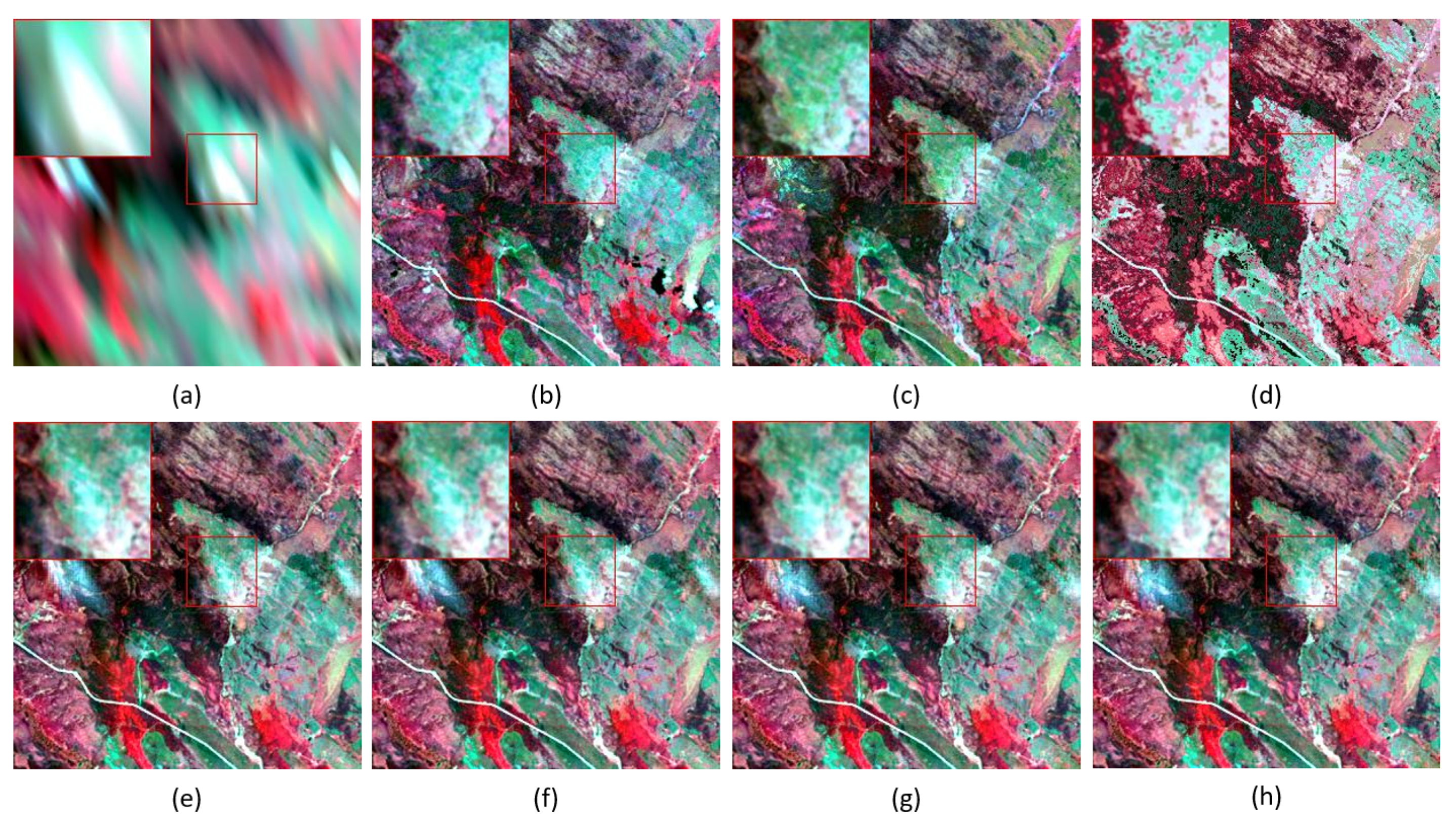
Figure 2 and Figure 3 compare the target (true) Landsat images with the images predicted by ESTARFM, CRSU, SPSTFM, EBSCDL, AMCFM and AMCFM-s. We use NIR-red-green band as the red-green-blue-band composite to show the images. These images are displayed with an ENVI 5.3 (Harris Geospatial Solutions, Broomfield, Colorado, United States) 2% linear enhancement.
All these fusion algorithms have the capability to reconstruct the main structure and details of the target image. It appears that the colors of the dictionary learning methods are visually more similar to the true Landsat image than the weighting method and unmixing-based method. The details captured by AMCFM are more prominent than those captured by SPSTFM and EBSCDL, which can be observed in the two-times enlarged red box in the images. Overall, our proposed method has the best performance in visualization.
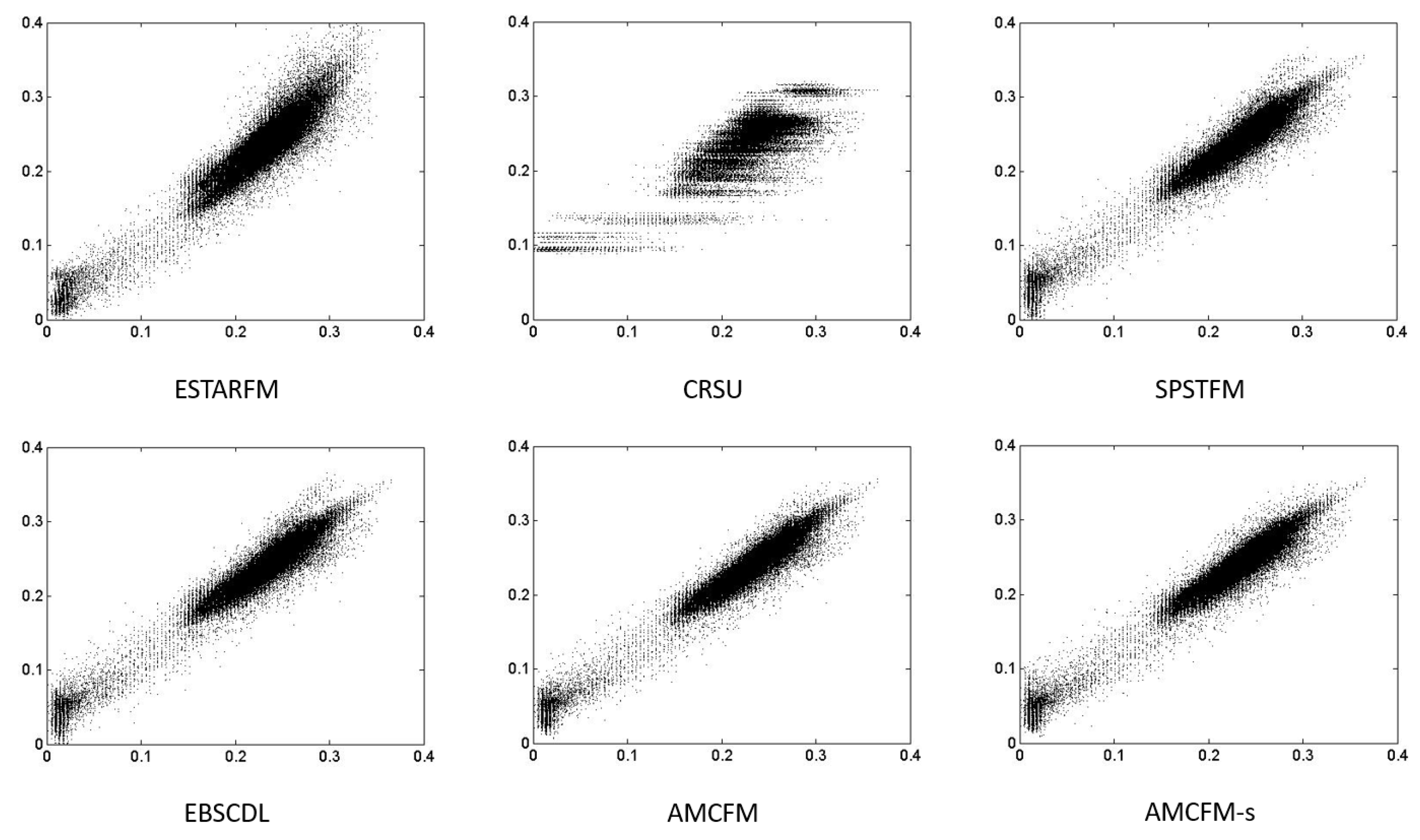
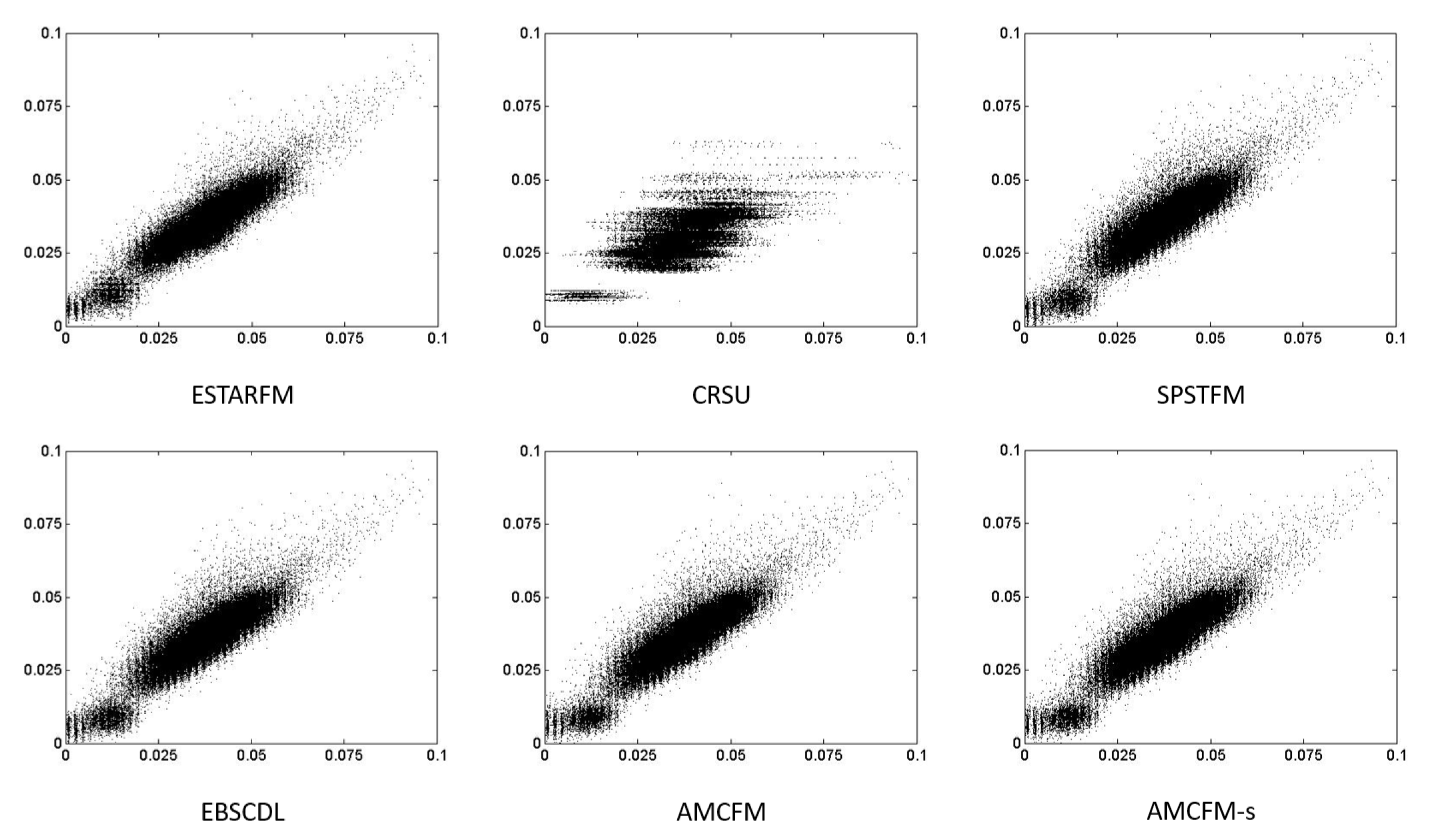
Figure 4, Figure 5 and Figure 6 display the 2D scatter plots of NIR, red and green band of image 1. ESTARFM performs slightly better than the other methods in the red band. This result is consistent with the statistics in Table 3. However, in the NIR and green band, it is obvious that dictionary learning methods outperform the weighting method and unmixing-based method because scatter plots of ESTARFM and CRSU are more dispersed. The scatter plots of our proposed methods, AMCFM and AMCFM-s, are closer to the 1-1 line than the other methods, indicating that using the edge information can actually improve fusion performance, especially in the NIR band. In general, Figure 4, Figure 5 and Figure 6 show that our proposed methods reconstruct images closest to the true Landsat image.
4. Discussion
Although the model performs well in the experiments, there still exists some questions to be discussed. Therefore, more experiments are performed to answer these questions.
4.1. Which Condition Is Better for AMCFM
Table 6, Table 7 and Table 8 show that image 1 best fits our model. This can be explained by the level of details in Table 9. We employ “” to represent the level of details of a target image as in [19]. It is clear that image 1 has the highest level of details in NIR band and the most similar levels of details in the three bands. Therefore, more structure similarity information can be captured to improve the fusion results. When there is a large divergence in a certain band, such as the red band in image 2, the results of the dictionary learning methods in this band are unsatisfactory. Under this situation, the ESTARFM performs better in red band.
4.2. Computational Cost
Computational cost is an important factor in practical application. Table 10 records the running time of all algorithms in image 1. It shows that SPSTFM has the fastest running speed. EBSCDL is time-consuming because the algorithm models the relationship between high and low resolution patches by a mapping function. AMCFM is a little slower than EBSCDL because of the complexity of the ADMM algorithm. However, for the improvement in results obtained, the slightly increased running time is acceptable. To accelerate the computation, an alternative approach can be designed to solve the reconstruction model efficiently, or the program can be coded with Graphics Processing Unit (GPU) support for parallel running in the future work.
4.3. Parameters
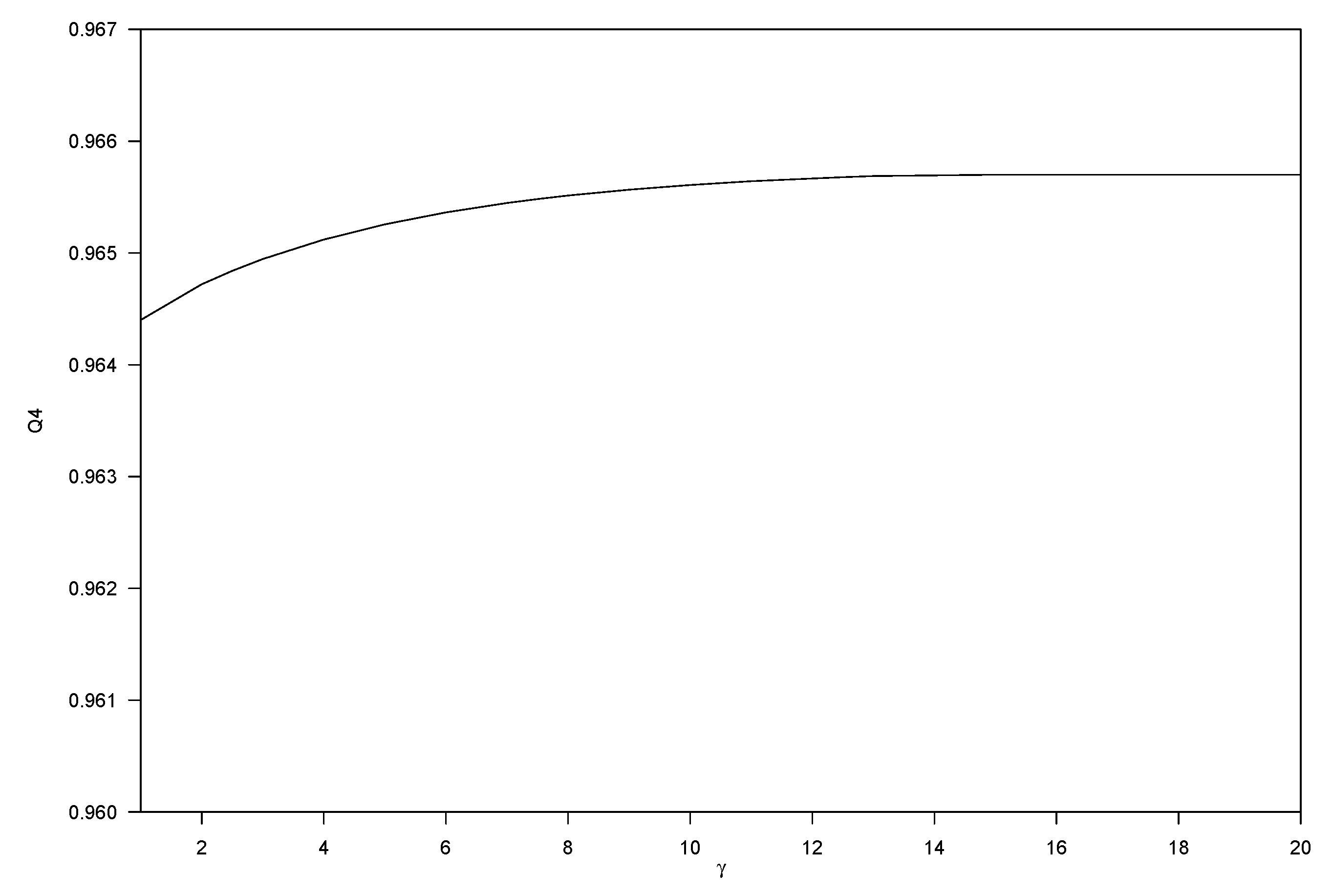
The parameters of the multi-band constraints determine the importance of the corresponding terms in the fusion model and the scalar affects the value of the parameter directly. In order to find a suitable , Figure 7 depicts how Q4 changes with respect to . Q4 is an index which encapsulates both spectral and radiometric measurements of the fusion result. Thus, we choose it to reflect the fusion results. A larger value of Q4 means a better fusion performance. When is smaller than 10, the performance of AMCFM evidently improves with the increase of . However, Q4 hardly increases when is larger than 10. Therefore, we set to 10.
5. Conclusions and Future Work
In this paper, we have proposed a novel dictionary learning fusion model, called AMCFM. This model considers the structure similarity between bands via adaptive multi-band constraints. These constraints essentially enforce the similarities of the edge information across bands in high resolution patches to improve the fusion performance. Moreover, different from existing dictionary learning models which only emphasize on sparsity, we use the nuclear norm as the regularization term to represent both sparsity and correlation. Therefore, our model can reduce the impact of inefficient dictionary pair and improve the representation ability of the dictionary pair. Comparing with four state-of-the-art fusion methods in metrics and visual effects, the experimental results support our proposed model in the improvements of image fusion. Although our model is slower than the other two dictionary learning methods in this empirical analysis because of the complexity of the optimization algorithm, the fusion results obtained from our model are improved indeed. One may wonder whether it is justifiable to achieve a slight improvement on the expense of an increase in computational time. Our argument is that, on a theoretical basis, our model is more reasonable and appealing than SPSTFM and EBSCDL because it capitalizes on the structure information and correlation of dictionaries for image fusion. Such advantages will be more evident when structure similarity increases.
However, there remains some room for improvement. Firstly, the norm loss term assumes that noise is an i.i.d. Gaussian. We can consider the use of other noise hypotheses, such as i.i.d. Gaussian mixture and non-i.i.d noise structure, to improve the fusion results. Secondly, the computation cost of the proposed method is high because of the complexity of the ADMM algorithm. To reduce the computation time, an alternative approach can be designed to solve the reconstruction model efficiently for practical applications. To analyze hyperspectral data efficiently, dimension reduction methods might need to be incorporated into the fusion process.
Author Contributions
H.Y., Y.L., F.C., T.F. and J.X. conceived the research and designed the experiments. H.Y., Y.L. and F.C. formulated the model and wrote the paper. H.Y. performed the experiments and interpreted the results with Y.L. and T.F. J.X. collected and processed the experimental data. All authors reviewed and approved the manuscript.
Funding
This research was funded by the earmarked grant CUHK 14653316 of the Hong Kong Research Grant Council.
Acknowledgments
The authors would like to thank the editor and reviewers for the valuable comments and suggestions on improving the manuscript.
Conflicts of Interest
The authors declare no conflict of interest.
References
- Townshend, J.; Justice, C.; Li, W.; Gurney, C.; McManus, J. Global land cover classification by remote sensing: Present capabilities and future possibilities. Remote Sens. Environ. 1991, 35, 243–255. [Google Scholar] [CrossRef]
- Loveland, T.R.; Shaw, D.M. Multiresolution land characterization: Building collaborative partnerships. In Gap Analysis: A Landscape Approach to Biodiversity Planning; Scott, J.M., Tear, T.H., Davis, F.W., Eds.; American Society for Photogrammetry and Remote Sensing: Bethesda, MD, USA, 1996; pp. 83–89. ISBN 978-5708303608. [Google Scholar]
- Vogelmann, J.E.; Howard, S.M.; Yang, L.; Larson, C.R.; Wylie, B.K.; Van Driel, N. Completion of the 1990s National Land Cover Data Set for the conterminous United States from Landsat Thematic Mapper data and ancillary data sources. Photogramm. Eng. Remote Sens. 2001, 67, 650–662. [Google Scholar]
- Pohl, C.; Van Genderen, J.L. Review article multisensor image fusion in remote sensing: Concepts, methods and applications. Int. J. Remote Sens. 1998, 19, 823–854. [Google Scholar] [CrossRef]
- Chen, B.; Huang, B.; Xu, B. Comparison of spatiotemporal fusion models: A review. Remote Sens. 2015, 7, 1798–1835. [Google Scholar] [CrossRef]
- Gao, F.; Masek, J.; Schwaller, M.; Hall, F. On the blending of the Landsat and MODIS surface reflectance: Predicting daily Landsat surface reflectance. IEEE Trans. Geosci. Remote Sens. 2006, 44, 2207–2218. [Google Scholar] [CrossRef]
- Zhu, X.; Chen, J.; Gao, F.; Chen, X.; Masek, J.G. An enhanced spatial and temporal adaptive reflectance fusion model for complex heterogeneous regions. Remote Sens. Environ. 2010, 114, 2610–2623. [Google Scholar] [CrossRef]
- Hilker, T.; Wulder, M.A.; Coops, N.C.; Linke, J.; McDermid, G.; Masek, J.G.; Gao, F.; White, J.C. A new data fusion model for high spatial-and temporal-resolution mapping of forest disturbance based on Landsat and MODIS. Remote Sens. Environ. 2009, 113, 1613–1627. [Google Scholar] [CrossRef]
- Li, H.; Manjunath, B.S.; Mitra, S.K. Multisensor image fusion using the wavelet transform. Graph. Models Image Process. 1995, 57, 235–245. [Google Scholar] [CrossRef]
- Nunez, J.; Otazu, X.; Fors, O.; Prades, A.; Pala, V.; Arbiol, R. Multiresolution-based image fusion with additive wavelet decomposition. IEEE Trans. Geosci. Remote Sens. 1999, 37, 1204–1211. [Google Scholar] [CrossRef] [Green Version]
- Miao, Q.G.; Shi, C.; Xu, P.F.; Yang, M.; Shi, Y.B. A novel algorithm of image fusion using shearlets. Opt. Commun. 2011, 284, 1540–1547. [Google Scholar] [CrossRef]
- Moigne, J.L.; Cromp, R.F. Wavelets for remote sensing image registration and fusion. In Wavelet Applications III; Szu, H.H., Ed.; SPIE-The International Society for Optical Engineering: Orlando, FL, USA, 1996; pp. 535–544. ISBN 978-0819421432. [Google Scholar]
- Czaja, W.; Doster, T.; Murphy, J.M. Wavelet packet mixing for image fusion and pan-sharpening. In Proceedings of the Algorithms and Technologies for Multispectral, Hyperspectral, and Ultraspectral Imagery XX, Baltimore, MD, USA, 5–9 May 2014; p. 908803. [Google Scholar]
- Deng, C.; Wang, S.; Chen, X. Remote sensing images fusion algorithm based on shearlet transform. In Proceedings of the 2009 International Conference on Environmental Science and Information Application Technology, Wuhan, China, 4–5 July 2009; pp. 451–454. [Google Scholar]
- Huang, B.; Song, H. Spatiotemporal reflectance fusion via sparse representation. IEEE Trans. Geosci. Remote Sens. 2012, 50, 3707–3716. [Google Scholar] [CrossRef]
- Wang, S.; Zhang, L.; Liang, Y.; Pan, Q. Semi-coupled dictionary learning with applications to image super-resolution and photo-sketch synthesis. In Proceeding of the 2012 IEEE Conference on Computer Vision and Pattern Recognition (CVPR), Providence, RI, USA, 16–21 June 2012; pp. 2216–2223. [Google Scholar]
- Wu, B.; Huang, B.; Zhang, L. An error-bound-regularized sparse coding for spatiotemporal reflectance fusion. IEEE Trans. Geosci. Remote Sens. 2015, 53, 6791–6803. [Google Scholar] [CrossRef]
- Wei, J.; Wang, L.; Liu, P.; Song, W. Spatiotemporal fusion of remote sensing images with structural sparsity and semi-coupled dictionary learning. Remote Sens. 2016, 9, 21. [Google Scholar] [CrossRef]
- Wei, J.; Wang, L.; Liu, P.; Chen, X.; Li, W.; Zomaya, A.Y. Spatiotemporal fusion of modis and landsat-7 reflectance images via compressed sensing. IEEE Trans. Geosci. Remote Sens. 2017, 55, 7126–7139. [Google Scholar] [CrossRef]
- Zurita-Milla, R.; Kaiser, G.; Clevers, J.G.P.W.; Schneider, W.; Schaepman, M.E. Downscaling time series of MERIS full resolution data to monitor vegetation seasonal dynamics. Remote Sens. Environ. 2009, 113, 1874–1885. [Google Scholar] [CrossRef]
- Wu, M.; Wu, C.; Huang, W.; Niu, Z.; Wang, C.; Li, W.; Hao, P. An improved high spatial and temporal data fusion approach for combining Landsat and MODIS data to generate daily synthetic Landsat imagery. Inf. Fusion 2016, 31, 14–25. [Google Scholar] [CrossRef]
- Amorós-López, J.; Gómez-Chova, L.; Alonso, L.; Guanter, L.; Zurita-Milla, R.; Moreno, J.; Camps-Valls, G. Multitemporal fusion of Landsat/TM and ENVISAT/MERIS for crop monitoring. Int. J. Appl. Earth Obs. Geoinf. 2013, 23, 132–141. [Google Scholar] [CrossRef]
- Doxani, G.; Mitraka, Z.; Gascon, F.; Goryl, P.; Bojkov, B.R. A spectral unmixing model for the integration of multi-sensor imagery: A tool to generate consistent time series data. Remote Sens. 2015, 7, 14000–14018. [Google Scholar] [CrossRef]
- Zhang, W.; Li, A.; Jin, H.; Bian, J.; Zhang, Z.; Lei, G.; Qin, Z.; Huang, C. An enhanced spatial and temporal data fusion model for fusing Landsat and MODIS surface reflectance to generate high temporal Landsat-like data. Remote Sens. 2013, 5, 5346–5368. [Google Scholar] [CrossRef]
- Xu, Y.; Huang, B.; Xu, Y.; Cao, K.; Guo, C.; Meng, D. Spatial and Temporal Image Fusion via Regularized Spatial Unmixing. IEEE Geosci. Remote Sens. Lett. 2015, 12, 1362–1366. [Google Scholar] [CrossRef]
- Xue, J.; Leung, Y.; Fung, T. A Bayesian data fusion approach to spatio-temporal fusion of remotely sensed images. Remote Sens. 2017, 9, 1310. [Google Scholar] [CrossRef]
- Shi, C.; Liu, F.; Li, L.; Jiao, L.; Duan, Y.; Wang, S. Learning interpolation via regional map for pan-sharpening. IEEE Trans. Geosci. Remote Sens. 2015, 53, 3417–3431. [Google Scholar] [CrossRef]
- Glasner, D.; Bagon, S.; Irani, M. Super-resolution from a single image. In Proceeding of the 12th IEEE International Conference on Computer Vision (ICCV), Kyoto, Japan, 29 September–2 October 2009; pp. 349–356. [Google Scholar]
- Khateri, M.; Ghassemian, H. A Self-Learning Approach for Pan-sharpening of Multispectral Images. In Proceedings of the IEEE International Conference on Signal and Image Processing Applications, Kuching, Malaysia, 12–14 September 2017; pp. 199–204. [Google Scholar]
- Zhu, Z.Q.; Yin, H.; Chai, Y.; Li, Y.; Qi, G.; Zhu, Z.Q. A novel multi-modality image fusion method based on image decomposition and sparse representation. Inf. Sci. 2017, 432, 516–529. [Google Scholar] [CrossRef]
- Mousavi, H.S.; Monga, V. Sparsity-based color image super resolution via exploiting cross channel constraints. IEEE Trans. Image Process. 2017, 26, 5094–5106. [Google Scholar] [CrossRef] [PubMed]
- Zhao, J.; Hu, H.; Cao, F. Image super-resolution via adaptive sparse representation. Knowl.-Based Syst. 2017, 124, 23–33. [Google Scholar] [CrossRef]
- Wang, J.; Lu, C.; Wang, M.; Li, P.; Yan, S.; Hu, X. Robust face recognition via adaptive sparse representation. IEEE Trans. Cybern. 2014, 44, 2368–2378. [Google Scholar] [CrossRef] [PubMed]
- Aharon, M.; Elad, M.; Bruckstein, A. K-SVD: An algorithm for designing overcomplete dictionaries for sparse representation. IEEE Trans. Signal Process. 2006, 54, 4311. [Google Scholar] [CrossRef]
- Obozinski, G.; Bach, F. Trace Lasso: A trace norm regularization for correlated designs. In Proceedings of the Advances in Neural Information Processing Systems 24 (NIPS 2011), Granada, Spain, 12–15 December 2011; pp. 2187–2195. [Google Scholar]
- Lin, Z.; Chen, M.; Ma, Y. The augmented lagrange multiplier method for exact recovery of corrupted low-rank matrices. arXiv, 2010; arXiv:1009.5055. [Google Scholar]
- Lin, Z.; Liu, R.; Su, Z. Linearized alternating direction method with adaptive penalty for low-rank representation. In Proceedings of the Advances in Neural Information Processing Systems 24 (NIPS 2011), Granada, Spain, 12–15 December 2011; pp. 612–620. [Google Scholar]
- Yang, J.; Yuan, X. Linearized augmented Lagrangian and alternating direction methods for nuclear norm minimization. Math. Comput. 2013, 82, 301–329. [Google Scholar] [CrossRef]
- Cai, J.F.; Candès, E.J.; Shen, Z. A singular value thresholding algorithm for matrix completion. SIAM J. Optim. 2010, 20, 1956–1982. [Google Scholar] [CrossRef]
- Ranchin, T.; Wald, L. Fusion of high spatial and spectral resolution images: The ARSIS concept and its implementation. Photogramm. Eng. Remote Sens. 2000, 66, 49–61. [Google Scholar] [CrossRef]
- Gevaert, C.M.; García-Haro, F.J. A comparison of STARFM and an unmixing-based algorithm for Landsat and MODIS data fusion. Remote Sens. Environ. 2015, 156, 34–44. [Google Scholar] [CrossRef]
- Alparone, L.; Baronti, S.; Garzelli, A.; Nencini, F. A global quality measurement of pan-sharpened multispectral imagery. IEEE Geosci. Remote Sens. Lett. 2004, 1, 313–317. [Google Scholar] [CrossRef]
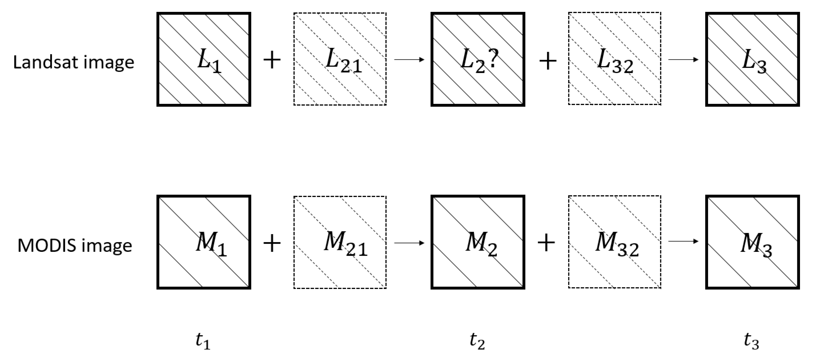
Figure 1.
Input images and the target image for spatiotemporal fusion (). Three low resolution images , and , and two high resolution images and are known. The high resolution image is the target image to be predicted.
Figure 1.
Input images and the target image for spatiotemporal fusion (). Three low resolution images , and , and two high resolution images and are known. The high resolution image is the target image to be predicted.

Figure 2.
Comparisons between the true image 1 and images reconstructed by different fusion methods. (a) MODIS (Moderate Resolution Imaging Spectroradiometer); (b) true Landsat image; (c) ESTARFM (Enhanced Spatial and Temporal Adaptive Reflectance Fusion Model); (d) CRSU (Class Regularized Spatial Unmixing); (e) SPSTFM (Sparse-representation-based Spatiotemporal Reflectance Fusion Model); (f) EBSCDL (Error-Bound-regularized Semi-Coupled Dictionary Learning); (g) AMCFM (adaptive multi-band constraints fusion model); (h) AMCFM-s.

Figure 3.
Comparisons between the true image 2 and images reconstructed by different fusion methods. (a) MODIS; (b) true Landsat image; (c) ESTARFM; (d) CRSU; (e) SPSTFM; (f) EBSCDL; (g) AMCFM; (h) AMCFM-s.
Figure 3.
Comparisons between the true image 2 and images reconstructed by different fusion methods. (a) MODIS; (b) true Landsat image; (c) ESTARFM; (d) CRSU; (e) SPSTFM; (f) EBSCDL; (g) AMCFM; (h) AMCFM-s.

Figure 4.
Scatter plots of NIR band of image 1. Abscissa is the true reflectance and ordinate is the predicted reflectance.
Figure 4.
Scatter plots of NIR band of image 1. Abscissa is the true reflectance and ordinate is the predicted reflectance.

Figure 5.
Scatter plots of red band of image 1. Abscissa is the true reflectance and ordinate is the predicted reflectance.
Figure 5.
Scatter plots of red band of image 1. Abscissa is the true reflectance and ordinate is the predicted reflectance.

Figure 6.
Scatter plots of green band of image 1. Abscissa is the true reflectance and ordinate is the predicted reflectance.
Figure 6.
Scatter plots of green band of image 1. Abscissa is the true reflectance and ordinate is the predicted reflectance.

Figure 7.
Relationship between Q4 and .


Table 1.
Mean and standard deviation in three bands of a multi-band image.
| Index | Image 1 | Image 2 | Image 3 | ||||||
|---|---|---|---|---|---|---|---|---|---|
| NIR | Red | Green | NIR | Red | Green | NIR | Red | Green | |
| Mean Value | 0.2212 | 0.0378 | 0.0483 | 0.2113 | 0.0345 | 0.0476 | 0.2320 | 0.0355 | 0.0487 |
| Standard Deviation | 0.0546 | 0.0105 | 0.0097 | 0.0383 | 0.0141 | 0.0121 | 0.0413 | 0.0108 | 0.0084 |
Table 2.
Bandwidth of Landsat and MODIS.
| Band Name | Landsat | MODIS | ||
|---|---|---|---|---|
| Band Number | Bandwidth (nm) | Band Number | Bandwidth (nm) | |
| Blue | 1 | 450–520 | 3 | 459–479 |
| Green | 2 | 530–610 | 4 | 545–565 |
| Red | 3 | 630–690 | 1 | 620–670 |
| Near-Infrared | 4 | 780–900 | 2 | 841–876 |
| Middle-Infrared | 5 | 1550–1750 | 6 | 1628–1652 |
| Middle-Infrared | 7 | 2090–2350 | 7 | 2105–2155 |
Table 3.
Band quality metrics in image 1.
| Approaches | RMSE | AAD | CC | ||||||
|---|---|---|---|---|---|---|---|---|---|
| NIR | Red | Green | NIR | Red | Green | NIR | Red | Green | |
| ESTARFM | 0.0177 | 0.0049 | 0.0043 | 0.0133 | 0.0039 | 0.0033 | 0.9553 | 0.9102 | 0.8951 |
| CRSU | 0.0286 | 0.0099 | 0.0071 | 0.0217 | 0.0084 | 0.0059 | 0.9050 | 0.7670 | 0.7975 |
| SPSTFM | 0.0157 | 0.0051 | 0.0040 | 0.0121 | 0.0040 | 0.0031 | 0.9717 | 0.8935 | 0.9148 |
| EBSCDL | 0.0157 | 0.0051 | 0.0040 | 0.0120 | 0.0040 | 0.0031 | 0.9721 | 0.8938 | 0.9152 |
| AMCFM | 0.0152 | 0.0050 | 0.0039 | 0.0118 | 0.0039 | 0.0030 | 0.9755 | 0.8979 | 0.9163 |
| AMCFM-s | 0.0154 | 0.0050 | 0.0039 | 0.0119 | 0.0039 | 0.0030 | 0.9743 | 0.8978 | 0.9158 |
RMSE, root mean square error; AAD, average absolute difference; CC, correlation coefficient.
Table 4.
Band quality metrics in image 2.
| Approaches | RMSE | AAD | CC | ||||||
|---|---|---|---|---|---|---|---|---|---|
| NIR | Red | Green | NIR | Red | Green | NIR | Red | Green | |
| ESTARFM | 0.0201 | 0.0109 | 0.0102 | 0.0133 | 0.0046 | 0.0045 | 0.8678 | 0.6488 | 0.5766 |
| CRSU | 0.0284 | 0.0120 | 0.0108 | 0.0215 | 0.0065 | 0.0054 | 0.7330 | 0.5436 | 0.4933 |
| SPSTFM | 0.0193 | 0.0110 | 0.0102 | 0.0125 | 0.0051 | 0.0044 | 0.8696 | 0.6508 | 0.5736 |
| EBSCDL | 0.0193 | 0.0110 | 0.0102 | 0.0125 | 0.0051 | 0.0044 | 0.8704 | 0.6515 | 0.5746 |
| AMCFM | 0.0189 | 0.0110 | 0.0102 | 0.0122 | 0.0051 | 0.0044 | 0.8756 | 0.6525 | 0.5730 |
| AMCFM-s | 0.0188 | 0.0110 | 0.0102 | 0.0121 | 0.0051 | 0.0044 | 0.8789 | 0.6509 | 0.5706 |
Table 5.
Band quality metrics in image 3.
| Approaches | RMSE | AAD | CC | ||||||
|---|---|---|---|---|---|---|---|---|---|
| NIR | Red | Green | NIR | Red | Green | NIR | Red | Green | |
| ESTARFM | 0.0194 | 0.0048 | 0.0049 | 0.0136 | 0.0036 | 0.0035 | 0.9136 | 0.8998 | 0.8366 |
| CRSU | 0.0285 | 0.0093 | 0.0064 | 0.0224 | 0.0073 | 0.0044 | 0.7965 | 0.6968 | 0.7251 |
| SPSTFM | 0.0165 | 0.0059 | 0.0040 | 0.0122 | 0.0044 | 0.0030 | 0.9276 | 0.8480 | 0.8859 |
| EBSCDL | 0.0164 | 0.0059 | 0.0040 | 0.0121 | 0.0044 | 0.0030 | 0.9280 | 0.8483 | 0.8861 |
| AMCFM | 0.0161 | 0.0057 | 0.0039 | 0.0120 | 0.0042 | 0.0029 | 0.9330 | 0.8583 | 0.8883 |
| AMCFM-s | 0.0162 | 0.0057 | 0.0040 | 0.0121 | 0.0042 | 0.0029 | 0.9324 | 0.8584 | 0.8878 |
Table 6.
Global quality metrics in image 1.
| Approaches | mRMSE | RASE | ERGAS | Q4 |
|---|---|---|---|---|
| ESTARFM | 0.0090 | 10.6579 | 0.6155 | 0.9515 |
| CRSU | 0.0152 | 17.5449 | 1.1343 | 0.8670 |
| SPSTFM | 0.0083 | 9.5958 | 0.6013 | 0.9628 |
| EBSCDL | 0.0083 | 9.5662 | 0.6002 | 0.9631 |
| AMCFM | 0.0080 | 9.2880 | 0.5866 | 0.9656 |
| AMCFM-s | 0.0081 | 9.4056 | 0.5884 | 0.9641 |
RASE, relative average spectral error; ERGAS, Erreur Relative Globale Adimensionnelle de Synthèse.
Table 7.
Global quality metrics in image 2.
| Approaches | mRMSE | RASE | ERGAS | Q4 |
|---|---|---|---|---|
| ESTARFM | 0.0137 | 14.7738 | 1.3645 | 0.8251 |
| CRSU | 0.0171 | 19.3090 | 1.5131 | 0.6519 |
| SPSTFM | 0.0135 | 14.4394 | 1.3702 | 0.8074 |
| EBSCDL | 0.0135 | 14.4177 | 1.3686 | 0.8080 |
| AMCFM | 0.0134 | 14.2524 | 1.3644 | 0.8113 |
| AMCFM-s | 0.0133 | 14.1951 | 1.3671 | 0.8116 |
Table 8.
Global quality metrics in image 3.
| Approaches | mRMSE | RASE | ERGAS | Q4 |
|---|---|---|---|---|
| ESTARFM | 0.0097 | 11.2841 | 0.6511 | 0.9025 |
| CRSU | 0.0147 | 16.8017 | 1.0984 | 0.7556 |
| SPSTFM | 0.0088 | 9.8227 | 0.6849 | 0.9117 |
| EBSCDL | 0.0088 | 9.8013 | 0.6840 | 0.9120 |
| AMCFM | 0.0086 | 9.5761 | 0.6652 | 0.9159 |
| AMCFM-s | 0.0086 | 9.6288 | 0.6658 | 0.9148 |
Table 9.
Level of details in a target image.
| Image 1 | Image 2 | Image 3 | |||||||
|---|---|---|---|---|---|---|---|---|---|
| NIR | Red | Green | NIR | Red | Green | NIR | Red | Green | |
| 0.2468 | 0.2777 | 0.2008 | 0.1812 | 0.4087 | 0.2542 | 0.1780 | 0.3042 | 0.1725 | |
Table 10.
Computational cost (in seconds).
| Time | ESTARFM | CRSU | SPSTFM | EBSCDL | AMCFM | AMCFM-s |
|---|---|---|---|---|---|---|
| training | - | - | 29 | 731 | 29 | 29 |
| predicting | 103 | 52 | 8 | 101 | 948 | 945 |
| total | 103 | 52 | 37 | 842 | 977 | 974 |
© 2018 by the authors. Licensee MDPI, Basel, Switzerland. This article is an open access article distributed under the terms and conditions of the Creative Commons Attribution (CC BY) license (http://creativecommons.org/licenses/by/4.0/).
Share and Cite
MDPI and ACS Style
Ying, H.; Leung, Y.; Cao, F.; Fung, T.; Xue, J. Sparsity-Based Spatiotemporal Fusion via Adaptive Multi-Band Constraints. Remote Sens. 2018, 10, 1646. https://0-doi-org.brum.beds.ac.uk/10.3390/rs10101646
AMA Style
Ying H, Leung Y, Cao F, Fung T, Xue J. Sparsity-Based Spatiotemporal Fusion via Adaptive Multi-Band Constraints. Remote Sensing. 2018; 10(10):1646. https://0-doi-org.brum.beds.ac.uk/10.3390/rs10101646
Chicago/Turabian StyleYing, Hanchi, Yee Leung, Feilong Cao, Tung Fung, and Jie Xue. 2018. "Sparsity-Based Spatiotemporal Fusion via Adaptive Multi-Band Constraints" Remote Sensing 10, no. 10: 1646. https://0-doi-org.brum.beds.ac.uk/10.3390/rs10101646
Note that from the first issue of 2016, this journal uses article numbers instead of page numbers. See further details here.