Global Fractional Vegetation Cover Estimation Algorithm for VIIRS Reflectance Data Based on Machine Learning Methods

Abstract

Fractional vegetation cover (FVC) is an essential input parameter for many environmental and ecological models. Recently, several global FVC products have been generated using remote sensing data. The Global LAnd Surface Satellite (GLASS) FVC product, which is generated from Moderate Resolution Imaging Spectroradiometer (MODIS) data, has attained acceptable performance. However, the original MODIS operation design lifespan has been exceeded. The Visible Infrared Imaging Radiometer Suite (VIIRS) onboard the Suomi National Polar-Orbiting Partnership (S-NPP) satellite was designed to be the MODIS successor. Therefore, developing an FVC estimation algorithm for VIIRS data is important for maintaining continuous FVC estimates in case of MODIS failure. In this study, a global FVC estimation algorithm for VIIRS surface reflectance data was proposed based on machine learning methods, which investigated the performances of back propagating neural networks (BPNNs), general regression networks (GRNNs), multivariate adaptive regression splines (MARS), and Gaussian process regression (GPR). The training samples were extracted from the GLASS FVC product and corresponding reconstructed VIIRS surface reflectance in 2013 over the global sampling locations. The VIIRS reflectances of red and near infrared (NIR) bands were the input variables for these machine learning methods. The theoretical performances and independent validation results indicated that the four machine learning methods could achieve similar and reliable FVC estimates. Regarding the FVC estimation accuracy, the GPR method achieved the best performance (R² = 0.9019, RMSE = 0.0887). The MARS method had the obvious advantage of computational efficiency. Furthermore, the FVC estimates achieved good spatial and temporal continuities. Therefore, the proposed FVC estimation algorithm for VIIRS data can potentially generate reliable global FVC data for related applications.

1. Introduction

Fractional vegetation cover (FVC), which is defined as the fraction of green vegetation seen from the nadir [1,2,3], is an important biophysical parameter for many environmental and ecological models. Large scale, long-term FVC data are critical for monitoring earth surface changes. Current global or regional FVC products are mainly derived from remote sensing data, such as the Polarization and Directionality of the Earth’s Reflectance (POLDER), Medium Resolution Imaging Spectrometer (MERIS), Spinning-Enhanced Visible and Infrared Imager (SEVIRI), Advanced Very High Resolution Radiometer (AVHRR), SPOT/VEGETATION and Moderate Resolution Imaging Spectroradiometer (MODIS) data [4,5,6,7]. However, it is well known that the MODIS sensor is aging, and the degradation and changes of onboard solar diffuser (SD) are also nonnegligible [8,9]. As a successor, the Visible Infrared Imaging Radiometer Suite (VIIRS) sensor onboard the Suomi National Polar-Orbiting Partnership (S-NPP) satellite was successfully launched in 2011 to collect visible and infrared imagery and radiometric measurements of the land, atmosphere, cryosphere, and oceans [10,11,12,13]. The VIIRS sensor, which is the second-generation of United States moderate-resolution imaging radiometer, extends and improves upon a series of measurements initiated by the MODIS sensor. For example, the VIIRS sensor has wider range of swath dimensions and better polarization performance than MODIS [8]. Also, the VIIRS sensor has fewer bands and different spectral coverage comparing with MODIS in the 0.4 to 1.0 μm spectral range [8]. The ground-test indicates that the radiometric performances of nadir Horizontal Sptial Resolution (HSR) and Noise Equivalent Temperature Difference (NEdT) between MODIS and VIIRS sensor are different when they are normalized to the same spatial scale and radiance level [8]. Since these changes and differences, the land surface parameter estimation algorithms or related methods for MODIS data should be reconsidered for VIIRS data. Therefore, several land surface parameter estimation algorithms were developed for VIIRS data, such as land surface albedo, leaf area index (LAI) and fraction of absorbed photosynthetically active radiation (FAPAR), to continue generating the corresponding datasets in case of MODIS failure [14,15]. However, no investigation has been conducted on global FVC estimation algorithm for VIIRS data until now. Thus, developing a global FVC estimation algorithm for VIIRS data to succeed the FVC estimation by MODIS data is significant and the main goal of this study.

The commonly used algorithms for FVC estimation from remote sensing data mainly include empirical methods, pixel unmixing models and machine learning methods [16,17,18]. Empirical methods are based on the relationship between FVC and vegetation indices or specific bands’ reflectances. Empirical methods require sufficiently representative and reliable training samples, and they can achieve a satisfactory performance on a regional scale. However, there may be increased uncertainties in FVC estimations using empirical methods when applied to large regions or different vegetation types [16], because the statistical relationships usually change with variations in ground surface conditions, such as different soil or vegetation types. Pixel unmixing models assume that each pixel is composed of several components, and the fraction of vegetation composition is considered to be the pixel FVC. The dimidiate pixel model, which is a popular pixel unmixing method, assumes that the pixel is only composed of vegetation and non-vegetation compositions [19,20,21,22]. The dimidiate pixel model is widely used in small regions with simple land surface conditions. However, the selection of representative endmembers for pixel unmixing methods might be difficult, especially when applied at large scales with complicated land surface conditions.

Recently, machine learning methods have also been widely used for FVC estimation and other vegetation parameter estimations on a large scale. Machine learning methods usually estimate vegetation parameters through training on samples composed of pre-processed reflectance and corresponding vegetation parameters, which are derived from the physical model simulations [23]. Machine learning methods are computationally efficient and robust against noisy data. In addition, machine learning methods can effectively fit the multivariate non-linear relationships, which make them popular choices for large scale FVC estimations [7,24]. Generally, it is difficult to apply empirical methods on large scale FVC estimation, because the relationship between FVC and remote sensing data could change with temporal and spatial conditions [23]. Also, for pixel unmixing models, the selection of representative endmembers and their spectral responses over large scale could be very difficult, as the land cover types and vegetation conditions are complicated [23]. As a result, machine learning methods are suitable candidates for global FVC estimation thanks to their robust performance and ability of nonlinear fitting [25,26]. Furthermore, most of the current global land surface parameter products are generated using machine learning methods and have achieved acceptable performances [7,11,23,27]. For example, back-propagation neural networks (BPNNs) were used to generate the Carbon Cycle and Change in Land Observational Products (CYCLOPES) and GEOV1 FVC products [7]; general regression neural networks (GRNNs) were used to estimate global FVC from MODIS surface reflectance [27]; multivariate adaptive regression splines (MARS) effectively achieved reliable FVC estimation accuracy for generating the Global LAnd Surface Satellite (GLASS) FVC product from MODIS data [23]; and Gaussian Process Regression (GPR) was employed to estimate chlorophyll concentration and achieved a satisfactory performance [28]. Thus, machine learning methods are good choices for the development of a global FVC estimation algorithm for VIIRS reflectance data.

The objective of this study is to develop a reliable global FVC estimation algorithm for VIIRS data based on machine learning methods. Because different machine learning methods may have different computational efficiencies and estimation accuracies, the performances of four commonly used machine learning methods were investigated in this study, which included BPNNs, GRNNs, MARS, and GPR. Firstly, the training samples were extracted from the reconstructed VIIRS surface reflectance data and the corresponding GLASS FVC data over the global sampling sites. Then, the training samples were refined and used to train the four machine learning methods with red and NIR band reflectances as input variables. After training process and theoretical performance analysis, temporal–spatial comparisons among these four methods were assessed as well. Furthermore, the accuracy performances of these four machine learning methods were evaluated with an independent validation case study in Heihe region, where the Advanced Spaceborne Thermal Emission and Reflection Radiometer (ASTER) and Compact Airborne Imaging Spectrometer (CASI) data were used to generate high spatial resolution FVC data based on field FVC measurements. Finally, the best method for estimating FVC from VIIRS data was determined.

2. Data and Preprocessing

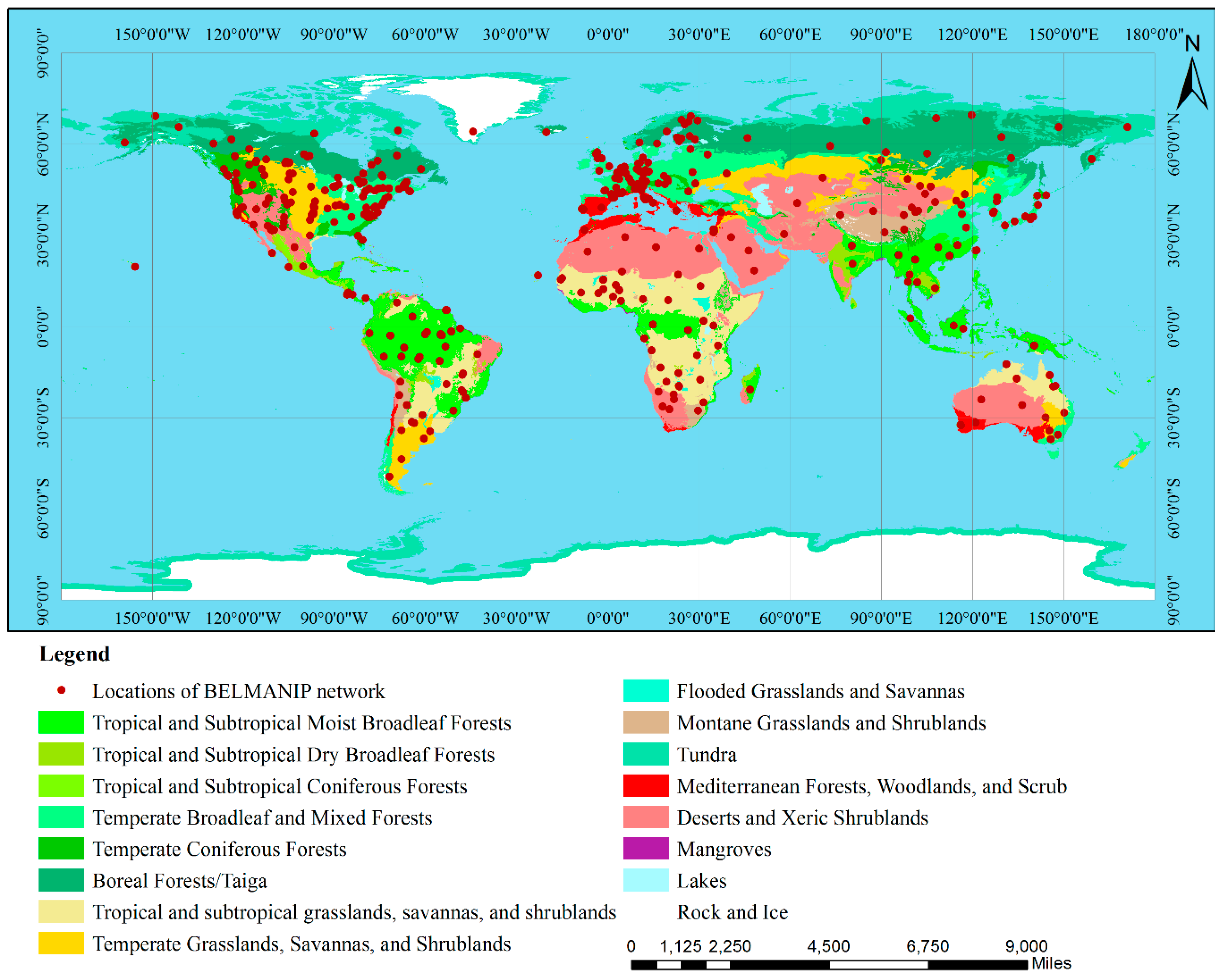
2.1. The BELMANIP Network

To develop the global FVC estimation algorithm for VIIRS data, representative training samples need to be generated firstly. Thus, choosing sampling locations with representativeness of different land cover types and vegetation conditions is essential for training sample generation. In this study, the Benchmark Land Multisite Analysis and Intercomparison of Products (BELMANIP) network was selected, because it had good spatial representativeness of biome types and conditions throughout the world [29]. The BELMANIP network had 402 sites, and their spatial distribution is presented in Figure 1, where all the sites distributed evenly over global terrestrial ecoregions (the statistic fractions of BELMANIP network sites with different surface components are provided by [29] and the map of terrestrial ecoregions is from [30]). The BELMANIP site locations were relatively flat and homogeneous with a kilometric resolution over 10 * 10 km² domains. Therefore, the BELMANIP sites were suitable for training sample generation and were used for developing the global FVC estimation algorithm for VIIRS data in this study.

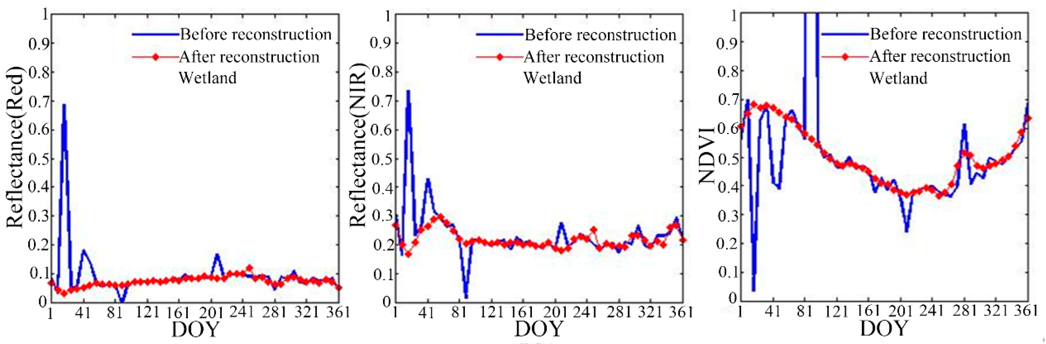
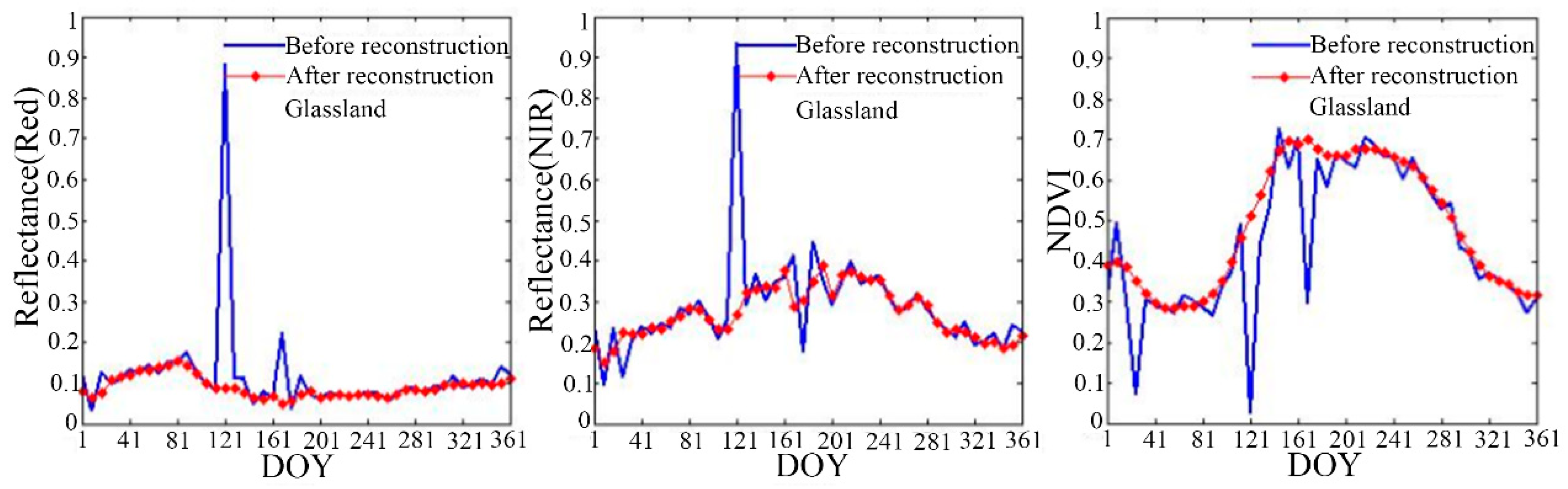
2.2. The VIIRS Surface Reflectance Data and Reconstruction

The VIIRS sensor onboard S-NPP satellite acquires Earth observation data for 22 spectral bands and wavelengths ranging from 0.3 to 14 μm, which includes ten visible and NIR reflective bands, eight short-wave infrared (SWIR) and mid-wave infrared (MWIR) bands, and four long-wave infrared (LWIR) bands [31]. For the spatial resolution of VIIRS data, there are 16 “Moderate” resolution (750 m) bands (M bands), five “Imagery” resolution (375 m) bands (I bands) and one low-light Day-Night-Band (750 m). The surface reflectance products are available in the “NPP Level 3 8-Day Tiled Products”, which contain three different spatial resolutions including 500 m, 1 km, and 5 km. In this study, integrated time series VIIRS surface reflectance data were needed to ensure that the training samples were representative of seasonal changes. Therefore, the 500 m spatial resolution reflectance products in 2013 were selected for VIIRS FVC estimation algorithm development. The temporal resolution of VIIRS data was 8-day, and there were 46 images for each tile per year. The dataset included three reflectance bands (red, NIR and SWIR) and a quality control band. The data were downloaded in “HDF” format from the website: https://ladsweb.modaps.eosdis.nasa.gov/search/.

The red and NIR band reflectances are the most sensitive variables for FVC estimation from remote sensing data. There is a strong relationship between the chlorophyll content and red band reflectance, which is one of the main chlorophyll absorption bands. The absorption of the red band will be strengthened when the chlorophyll content increases with the increasing FVC, which leads to a reflectance decrease in the red band. Meanwhile, the NIR band reflectance will increase when the FVC increases because this usually leads to a higher LAI and lower soil visibility. A higher LAI will cause higher reflectance, which is averse to that in the red band reflectance, but the transmittance obviously decreases along with the LAI [32]. Therefore, it is reasonable to estimate FVC using the red and NIR band reflectances, which are also selected to develop the global FVC estimation algorithm for VIIRS data in this study.

Though the VIIRS reflectance products have been atmospherically corrected, they may still contain abnormal values due to contaminations from residual clouds and undetected cloud shadows [33]. The anomalies of VIIRS reflectance data can bring large uncertainties to FVC estimation and cause an accuracy decrease in FVC estimation. Therefore, it is necessary to reprocess the VIIRS reflectance data to obtain high-quality reflectance data with fewer uncertainties. To remove the contaminated values and obtain high-quality VIIRS reflectance data, the method incorporating upper envelopes of time series Vegetation Indexes (VIs) as constraint conditions to Reconstruct time series of surface Reflectance (referred to VIRR), which was proposed for MODIS reflectance data reconstruction, was selected to reconstruct the time series VIIRS reflectance in this study [33]. First, the VIRR method is applied to calculate the normalized difference vegetation index (NDVI) (Formula (1)) using the NIR and red band reflectances. Then, the continuous upper envelopes of NDVI were calculated using the smoothing method developed by Garcia [34], which was a penalized least square regression method based on a three-dimensional discrete cosine transform (DCT-PLS). Cloud-contaminated reflectance values were detected using the time series NDVI and the upper envelopes of the time series NDVI. The surface reflectance data were then reconstructed using the cloud-free reflectance values by incorporating the continuous and smooth upper envelopes of time series NDVI as constraint conditions [33].

$$NDVI=\frac{R_{NIR}-R_{Red}}{R_{NIR}+R_{Red}}$$

(1)

where $R_{NIR}$ and $R_{Red}$ are the NIR and red band reflectances of the VIIRS data, respectively.

2.3. The GLASS FVC Data

The GLASS FVC product is a product extended from the GLASS product suite, which is generated from MODIS data under the support of China’s National High Technology Research and Development Program [27,35,36]. GLASS FVC was spatially and temporally compared with the GEOV1 FVC product, which was considered to have the best accuracy among all large scale FVC products by correcting the systematic error in the CYCLOPES FVC before the GLASS FVC was generated. The comparison results indicated that the GLASS FVC had comparable performances with the GEOV1 FVC product, and the temporal and spatial continuities of the GLASS FVC were much better than GEOV1 FVC [27]. The FVC estimation accuracies for GLASS and GEOV1 FVC were also directly compared using field measurement-based validation data from 44 Validation of Land European Remote Sensing Instruments (VALERI) sites. The direct validation results indicated that the GLASS FVC had comparable accuracy to the GEOV1 FVC [27]. Therefore, considering the direct validation performances of GLASS FVC and its better spatial and temporal continuities, the GLASS FVC data are believed to be suitable and reliable choices for generating time series training samples, which are used to develop the global FVC estimation algorithm for VIIRS data to succeed the MODIS data for FVC estimation. Furthermore, the GLASS FVC product has a 500 m spatial resolution, 8-day temporal resolution and sinusoidal grid projection, which are same as the VIIRS data. In this study, the GLASS FVC data from 2013, which correspond to the VIIRS surface reflectance, are selected as reference data for training sample generation.

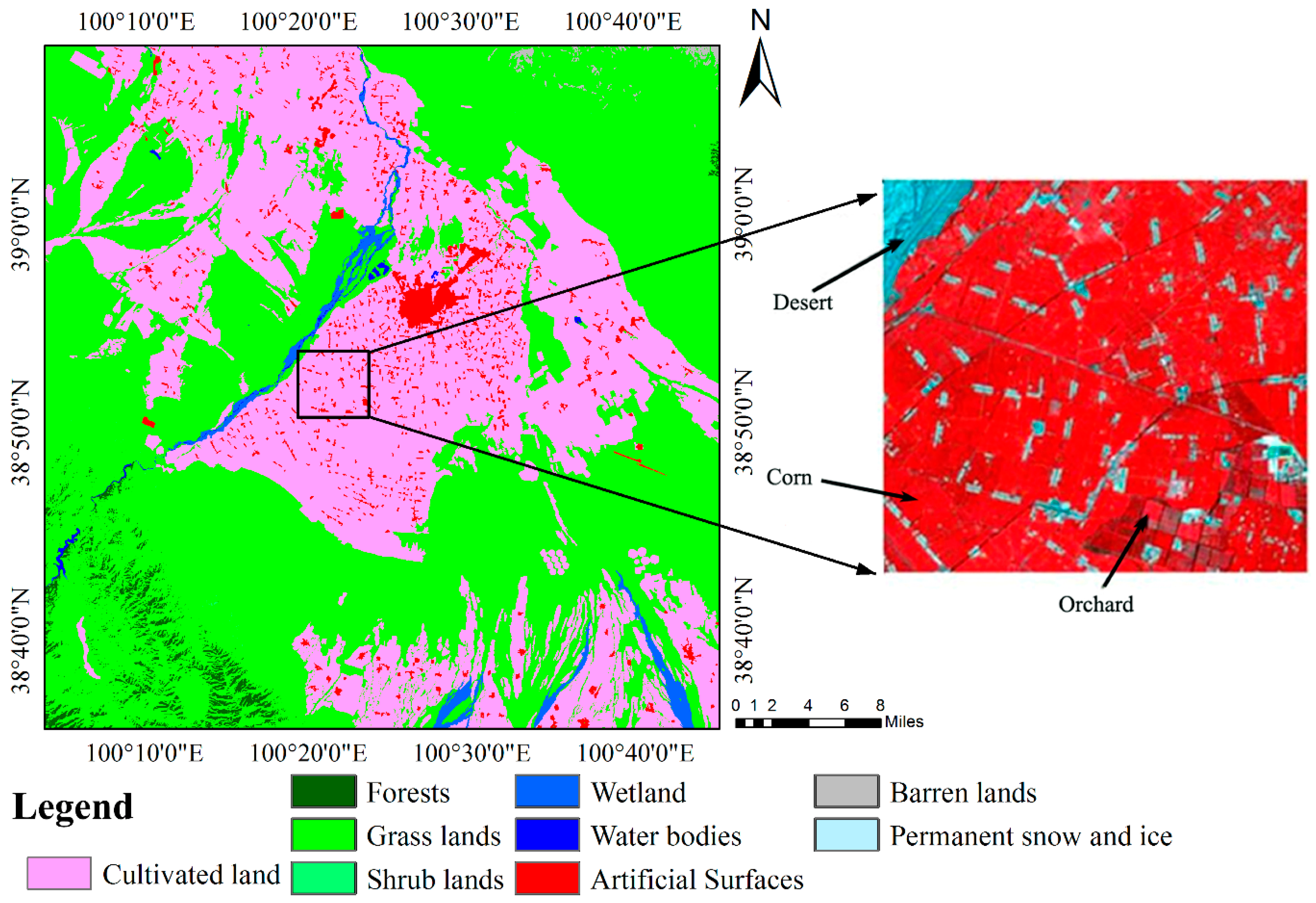
2.4. An Independent Validation Case in Heihe Region

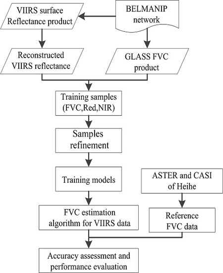
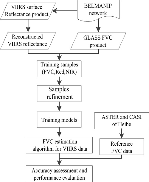
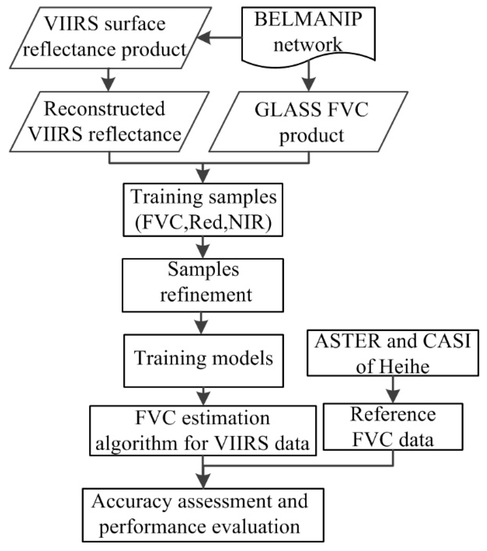
To evaluate the accuracy of FVC estimates from VIIRS data, an independent validation was conducted in Heihe region of China (Lat: 38°50′45″N to 38°53′30″N, Lon: 100°20′20″E to 100°24′0″E). The Heihe region is a relatively flat area and mainly covered with maize. Figure 2 shows the location and main land types of the study area. In this case study, high-spatial-resolution ASTER and CASI data (

Table 1. ASTER and Compact Airborne Imaging Spectrometer (CASI) data used in this study.

Data Type	Spatial Resolution	Acquisition Dates
ASTER	15 m	05/30, 06/15, 06/24, 07/10, 08/02, 08/11, 08/18, 08/27, 09/03
CASI	1 m	06/29, 07/07

) were used to upscale the ground FVC measurements. The field FVC measurements were conducted between May and September in 2012, which covered the whole maize growing season [37]. Twenty-two sampling sites with areas of approximately 10 m × 10 m each were selected throughout the region based on the land cover distribution, and sixteen of them were in maize fields. At each sampling site, nine digital photographs were taken along with two diagonals of the squared sampling site. Then the average of the FVC estimates from the nine photographs was considered to be the FVC value of the sampling site. The FVC of a photograph was defined as the percentage of vegetation pixels of the total number of pixels in the digital photograph. The FVC of each photograph was determined using a Gaussian simulation and segmentation method of the Commission Internationale de L’Eclairage (CIE) L∗a∗b∗ color space, which was an automatic, accurate and reliable method for FVC extraction from digital photographs with varying backgrounds and shadow conditions [38,39].

The empirical transfer functions (Formula (2)) between the field survey FVC data and NDVI calculated from the ASTER and CASI canopy reflectance data were generated and used to estimate high-spatial resolution FVC data, which were used as the independent validation FVC data for evaluating FVC estimates from VIIRS data [37,41].

$$FVC={\left(a\ast NDVI+b\right)}^k$$

(2)

where a, b and k were the coefficients determined by the NDVI of ASTER and CASI data and the corresponding field survey FVC data ([37] provides the detailed information about the field FVC measurement, as well as the ASTER/CASI FVC generation process and its accuracy). Finally, the FVC values of each VIIRS FVC pixel were directly compared with the averaged FVC values of pixels in the high spatial resolution FVC maps, which spatially matched that of the VIIRS FVC pixel.

3. Methods

The global FVC estimation algorithm flowchart for VIIRS surface reflectance data is shown in Figure 3. First, the VIRR method is used to reconstruct the time series VIIRS surface reflectance to obtain high-quality reflectance data. The BELMANIP network providing global sampling locations is used to extract FVC samples from the GLASS FVC data as well as the red and NIR band reflectances from the reconstructed VIIRS surface reflectance data. Then, the sample data are refined based on the approximate linear relationship between the FVC and VIIRS NDVI. Next, the four machine learning methods are trained with the training samples using red and NIR band reflectances as the input variables. Finally, the different machine learning method performances are evaluated.

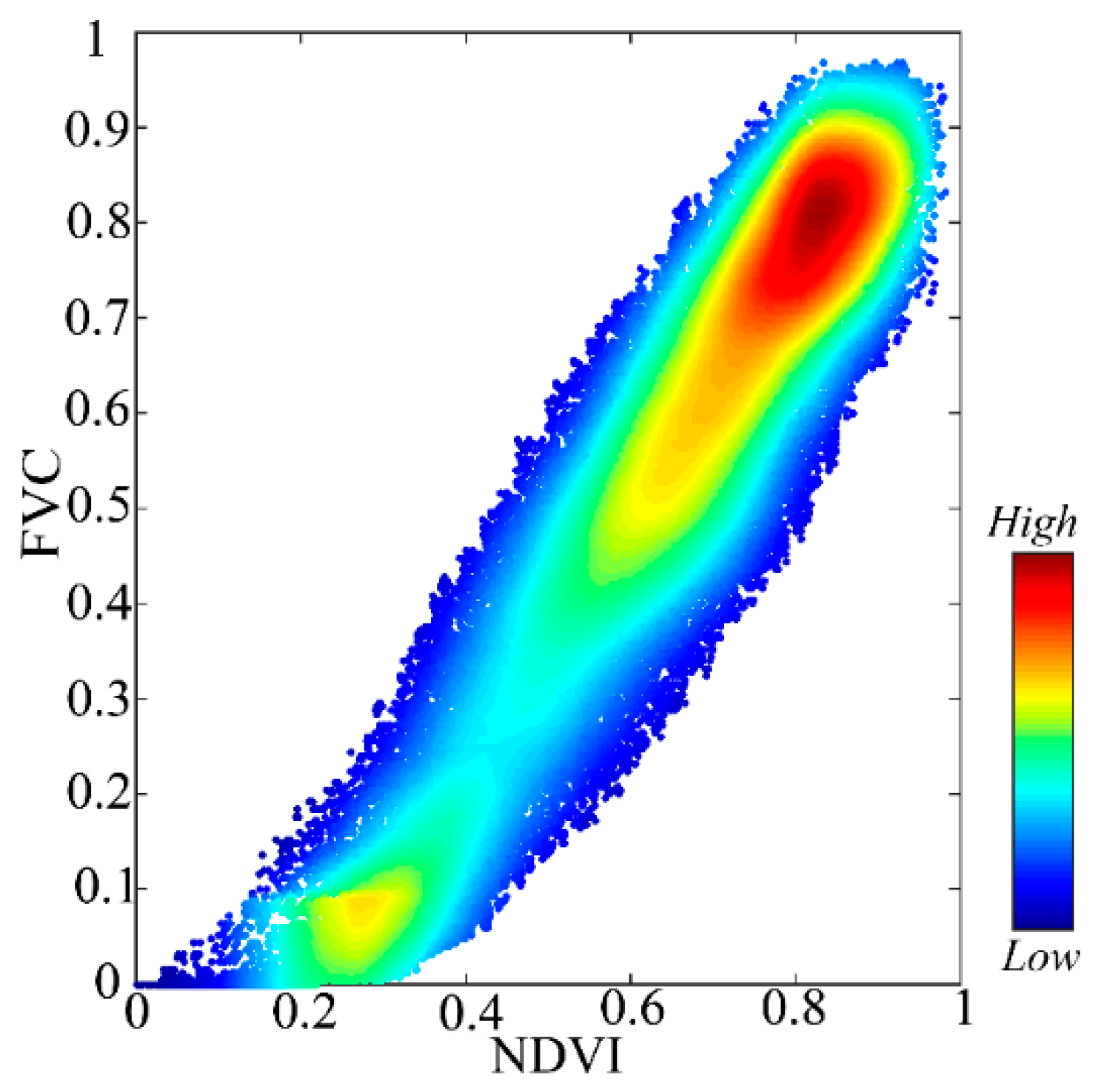
3.1. Training Samples Selection

The sample data contain the reconstructed VIIRS surface reflectance data and the corresponding FVC from the GLASS FVC product. The VIIRS reflectance data and GLASS FVC data have the same projections, as well as spatial and temporal resolutions. Therefore, the red and NIR band reflectances and corresponding FVC values can be easily extracted from the same pixel points in the VIIRS and GLASS FVC data. In this study, the samples were extracted from a 2 × 2 (1 km × 1 km) subset at each BELMANIP site of each tile, and there were 46 total tiles for the year 2013. The NDVI values of the same pixels corresponding to the GLASS FVC at the BELMANIP sites were also calculated from the reconstructed VIIRS surface reflectance.

The sample data were adequate but there might be uncertainties in the GLASS FVC or reconstructed VIIRS surface reflectances. Therefore, some abnormal FVC or surface reflectance values might exist in the sample data, which may increase uncertainties in machine learning method training and directly affect the accuracy of FVC estimates. Thus, sample data were further refined according to the approximately linear relationship between NDVI and FVC. In this study, the samples were divided into 100 classes, according to the VIIRS NDVI over a variation domain of [0, 1.0], and the GLASS FVC values lower than 15th percentile or higher than 85th percentile were removed from the sample datasets. Finally, 70% of the refined sample data were randomly selected as the training samples and the other 30% were used to validate the theoretical performances of the algorithm.

3.2. BPNNs

BPNNs is one type of artificial neural network that is widely adopted for estimating land surface vegetation parameters [7,18,42]. BPNNs contain three layers, which are the input, hidden and output layers. There are two procedures in the training of BPNNs, which include a forward propagation of information and a backward propagation of error [23]. First, the input values of training samples are fed into the input layer, and the estimated values are calculated through the forward propagation. Then, the weights in each successive layer would be adjusted based on the differences between the estimated and expected values to reduce the errors at each level. The information transmission procedure is a unidirectional transmission to the input layer, hidden layer, and transmission to the output layer [23]. Each layer’s status is only affected by the previous layer. In this study, the input variables for BPNNs were the reconstructed VIIRS surface reflectances of the red and NIR bands, while the output variable was the corresponding FVC. The BPNNs training was carried out using the MATLAB 2015b platform.

The numbers of the hidden layer and nodes in each hidden layer are the main parameters, which could directly affect the BPNNs accuracy. In this study, first, several experiential formulas (Formulas (3)–(5)) were used to obtain the primary ranges of the parameters and generate the BPNNs general structure [43]. Then, the optimal parameters were determined by adjusting the numbers of the hidden layer and nodes in each hidden layer based on the validation results. Furthermore, different activation functions, transfer functions and training functions were also evaluated to obtain the optional neural networks.

$$l<n-1$$

(3)

$$l<\sqrt{\left(m+n\right)}+a$$

(4)

$$l=lo{g}_{2}n$$

(5)

where $l$ is the number of nodes in the hidden layer, $n$ is the number of nodes in the input layer, which is 2 in this study, and $m$ is the number of nodes in the output layer, which is 1 in this study. $a$ is a constant between 0 and 10.

3.3. GRNNs

The GRNNs method is a generalization of the radial basis function and probabilistic neural networks, which was developed by Donald Specht [42,44]. There are pattern and summation layers in the GRNNs instead of hidden layer in the BPNNs. To train the GRNNs, the input data, which included the red and NIR band reflectances of the VIIRS data, were first put into the input layer and the number of neurons for the input layer was equal to the input data dimension. Then, the pattern layer calculated the distances between the observed reflectance data and known reflectance data from the training samples. The number of neurons for the pattern layer was dependent on the training sample quantity. The output data of the pattern layer were summated in the summation layer. Finally, the output layer computed the predicted FVC value by normalization. A Gaussian function was selected as the kernel function in the GRNNs, and its fundamental formulations were expressed as follows:

$$Y^{\prime }\left(X\right)=\frac{{\sum }_{i=1}^n{Y}^i\exp \left(-\frac{D_i^2}{2{\sigma }^2}\right)}{{\sum }_{i=1}^n\exp \left(-\frac{D_i^2}{2{\sigma }^2}\right)}$$

(6)

$$D_i^2={\left(X-X^i\right)}^T\left(X-X^i\right)$$

(7)

where $X$ represents the observed reflectance data, which were used to estimate the corresponding FVC value $Y^{\prime }\left(X\right)$, $X^i$ and $Y^i$ represent the ith known reflectance and corresponding FVC data from the training samples, $D_i^2$ represents the squared Euclidean distance between $X$ and $X^i$, n is the number of samples, and $\sigma$ is the smoothing parameter that controls the size of the receptive region. The weights and architecture would be adjusted automatically through the input value and the objective of training GRNNs was to obtain the optimized smoothing parameter σ [27]. In this study, the smoothing parameter was gradually changed by 0.001 from 0 to 1, and ten-fold cross-validation was used to find the optimal parameter.

3.4. MARS

MARS, developed by Jerome H. Friedman in 1991, is a regression analysis model, which could fit a piecewise linear function and address the nonlinear regression [45], particularly for high-dimensional data. The main process for training MARS is fitting a piecewise linear function to create a non-linearity model using the following form [45]:

$$f\left(x\right)={\displaystyle \sum }_{i=1}^k{c}_i{B}_i\left(x\right)$$

(8)

where $B_i\left(x\right)$ is the $i$th piecewise linear basis function, $c_i$ is the constant coefficient for the corresponding basis function. $x$ is the input vector data and $f\left(x\right)$ is the corresponding estimation. In this study, the input data included the red and NIR band reflectances and the corresponding FVC was the MARS model output. Every piecewise linear basis function in Formula (8) is created by taking the following form:

$$\max \left(0,x-c\right), x-c>0 \mathrm{or}\max \left(0,c-x\right), c-x>0$$

(9)

where $c$ is the knot parameter.

There are two steps to build the optimal MARS model. First, a group of basis functions are constructed to fit the relationship between the reflectances and FVC, which is based on the training samples. The selected data entered into the model can interact with each other or restricted to only be entered as assistive components. Second, basis functions are removed in the order of least contribution based on the generalized cross-validation (GCV) criterion [46]. When a variable was removed from the model, its contribution could be assessed through observing the decrease in calculated GCV. In this study, the MARS method was implemented using the ARESLab proposed by Jerome Friedman, which was a MATLAB toolbox for building a piecewise-linear and piecewise-cubic regression model using the MARS model (http://www.cs.rtu.lv/jekabsons/regression.html).

3.5. GPR

GPR is a probabilistic method, which is based on the GP learning framework and suitable for fitting a non-linear relationship [28,47]. The main target of GPR is to obtain the best estimates with the predictive distribution of sample data. GPR assumes that all variables conform to a Gaussian distribution (Formula (10)).

$$f~GP\left(m,k\right)$$

(10)

where $m$ and $k$ represent the mean function and covariance function respectively, and $f$ represents the distribution function. The relationship between the input and output data of GPR model is assumed as follows: $y=f\left(x\right)+\epsilon$, where the input data x and output data y are the VIIRS reflectance data and FVC values in this study, and $\epsilon$ is the Gaussian noise. Based on the GP learning framework, the output value $y$ is the sum of the distribution function $f$ and the noise component $\epsilon$. Thus, the prior distribution of known samples is modeled using Formula (11) [28]. To obtain the estimated values, the joint distribution of known samples and predicted data is necessary. Thanks to the assumption of the GP theory and marginalization property, the joint distribution is Gaussian and it can be expressed as Formula (12).

$$y~N\left(0,K\left(X,X\right)+{\sigma }_n^2{I}_n\right)$$

(11)

$$\left[\begin{array}{c}y\\ f_{\ast }\end{array}\right]~N\left(0,\left[\begin{array}{cc}K\left(X,X\right)+{\sigma }_n^2{I}_n& K\left(X,x_{\ast }\right)\\ K\left(x_{\ast },X\right)& k\left(x_{\ast },x_{\ast }\right)\end{array}\right]\right)$$

(12)

where $X$ and $y$ represent the known training sample data, which are the VIIRS red and NIR band reflectances as well as the corresponding FVC; $x_{\ast }$ represents the observed reflectance data, which were used to estimate the corresponding FVC value $f_{\ast }$; ${\sigma }_n^2$ represents the variance of noise; $K\left(X,X\right)$ is the auto-covariance matrix of known reflectance data $X$; $K\left(x_{\ast },X\right)$ and $K\left(X,x_{\ast }\right)$ are the covariance values of known reflectance data $X$ and observed reflectance data $x_{\ast }$; and $k\left(x_{\ast },x_{\ast }\right)$ is the auto-covariance matrix of the observed reflectance data $x_{\ast }$. According to the properties of Gaussian distribution, the predicted value and its variance is calculated as follows [28,47]:

$$f_{\ast }=K\left(x_{\ast },X\right){\left[K\left(X,X\right)+{\sigma }_n^2{I}_n\right]}^{-1}y$$

(13)

$$cov\left(f_{\ast }\right)=k\left(x_{\ast },x_{\ast }\right)-K\left(x_{\ast },X\right){\left[K\left(X,X\right)+{\sigma }_n^2{I}_n\right]}^{-1}K\left(X,x_{\ast }\right)$$

(14)

$f_{\ast }$ is the final estimated FVC and $cov\left(f_{\ast }\right)$ is the variance of the predicted value (see reference [47] for more details). The mean function and covariance function are the main parameters for the GPR method, which can directly affect the performance of this method. In this study, the initial mean function was set to zero to reduce the hyper-parameter. Different covariance functions from MATLAB 2015b were evaluated and the function with the minimum error was adopted.

4. Results

4.1. The VIIRS Reflectance Data Reconstruction

The VIIRS surface reflectance data were reconstructed using the VIRR method, and the reconstructed time series VIIRS surface reflectance data were evaluated at the BELMANIP sites. This method performed well on the time series VIIRS surface reflectance and NDVI reconstruction. Two sites were randomly selected from the 402 sampling sites to show the performance of the VIRR method (Figure 4 and Figure 5). Figure 4 and Figure 5 showed the time series profiles of the VIIRS surface reflectance in the red and NIR bands, as well as the NDVI values before and after reconstruction by VIRR method in 2013. The land cover types of the selected sites were wetland and grassland according to the MODIS land cover product (MCD12Q1).

The figures show evident abnormalities that change suddenly with time in the original VIIRS surface reflectance data as well as the NDVI profiles. These abnormalities may be caused by residual clouds, which do not conform to the vegetation growth rhythm. The reconstructed VIIRS surface reflectance effectively eliminated the abnormal values, and the VIRR algorithm performed well for reconstructing the time series VIIRS surface reflectance data. Therefore, the reflectance data reconstruction process could effectively improve the quality of VIIRS reflectance data, which was significant for improving FVC estimation accuracy.

4.2. Training Samples

The total number of final selected training samples was 52,368. Figure 6 shows the density scatter plots of the NDVI from the VIIRS data and the GLASS FVC values for the refined training samples. The approximate linear relationship between NDVI and FVC in Figure 6 indirectly indicated the training sample reliability. In addition, the relationship between GLASS FVC and VIIRS NDVI in Figure 6 was not strictly linear. The same NDVI may correspond to different FVC in a certain range, because the red and NIR band surface reflectances used to calculate the NDVI were usually different. Also, because of the spectral diversity, when the FVC value was the same, the spectral information varied from different green vegetation.

4.3. Theoretical Performances of Machine Learning Methods

The optimal model parameters of these machine learning methods were determined based on the training samples. For BPNNs, two hidden layers were determined and the optimal number of nodes for each hidden layer were 30 and 15, respectively. The optimal activation function of the hidden layer was “tansig”, the transfer function for output layer was “logsig”, and the training function was “traingdx”. For GRNNs, the optimal smoothing parameter was 0.005 in this study. The resulting optimal parameters for the MARS model in this study are shown in

Table 2. The optimal parameters for the multivariate adaptive regression splines (MARS) model.

Parameter	maxFuncs	C	Threshold
Value	201	3	1.0 × 10−4

“maxFuncs” represents the maximum number of basis functions. “C” is the penalty parameter and “threshold” is the threshold value.

. Regarding the GPR model, the optimal covariance function was “matern32”.

Four machine learning methods were trained using the 70 percent training samples, and their theoretical performances (

Table 3. The theoretical performances of the four machine learning methods (x and y represent the estimated FVC and GLASS FVC, respectively)

Models	RMSE	R2	Computational Time (s)	Statistical Formula
BPNNs	0.0909	0.8973	0.0172	y = 0.8853x + 0.0603
GRNNs	0.0893	0.9006	19.4393	y = 0.9013x + 0.0503
MARS	0.0891	0.9011	0.0089	y = 0.9972x − 0.0004
GPR	0.0887	0.9019	9.4425	y = 0.9041x + 0.0489

) were evaluated using R-square (R²), computational efficiency and root mean square error (RMSE), which were based on the same validation samples. These validation samples include all vegetation types on the land surface, thus the validation results have representativeness. The results indicated that the performances of the four machine learning methods were all satisfactory (RMSE < 0.1, R² > 0.85), especially for the GPR method, which achieved the best performance (RMSE = 0.0887, R² = 0.9019). The satisfactory results indicated that all the machine learning methods had potential for global FVC estimation using VIIRS data. The computational efficiency is another important factor for global FVC estimation using VIIRS data. Obviously, the computation efficiencies of BPNNs and MARS were superior to GRNNs and GPR. Therefore, these two methods were appropriate when the generation of huge FVC data was required.

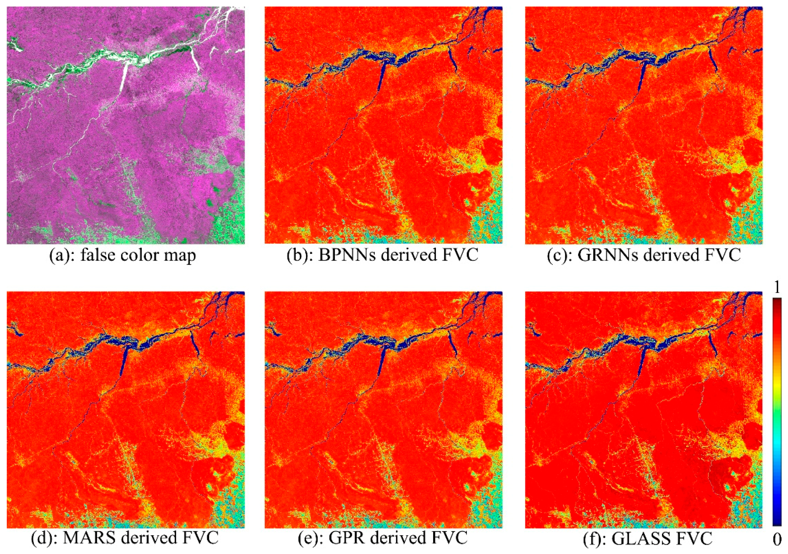
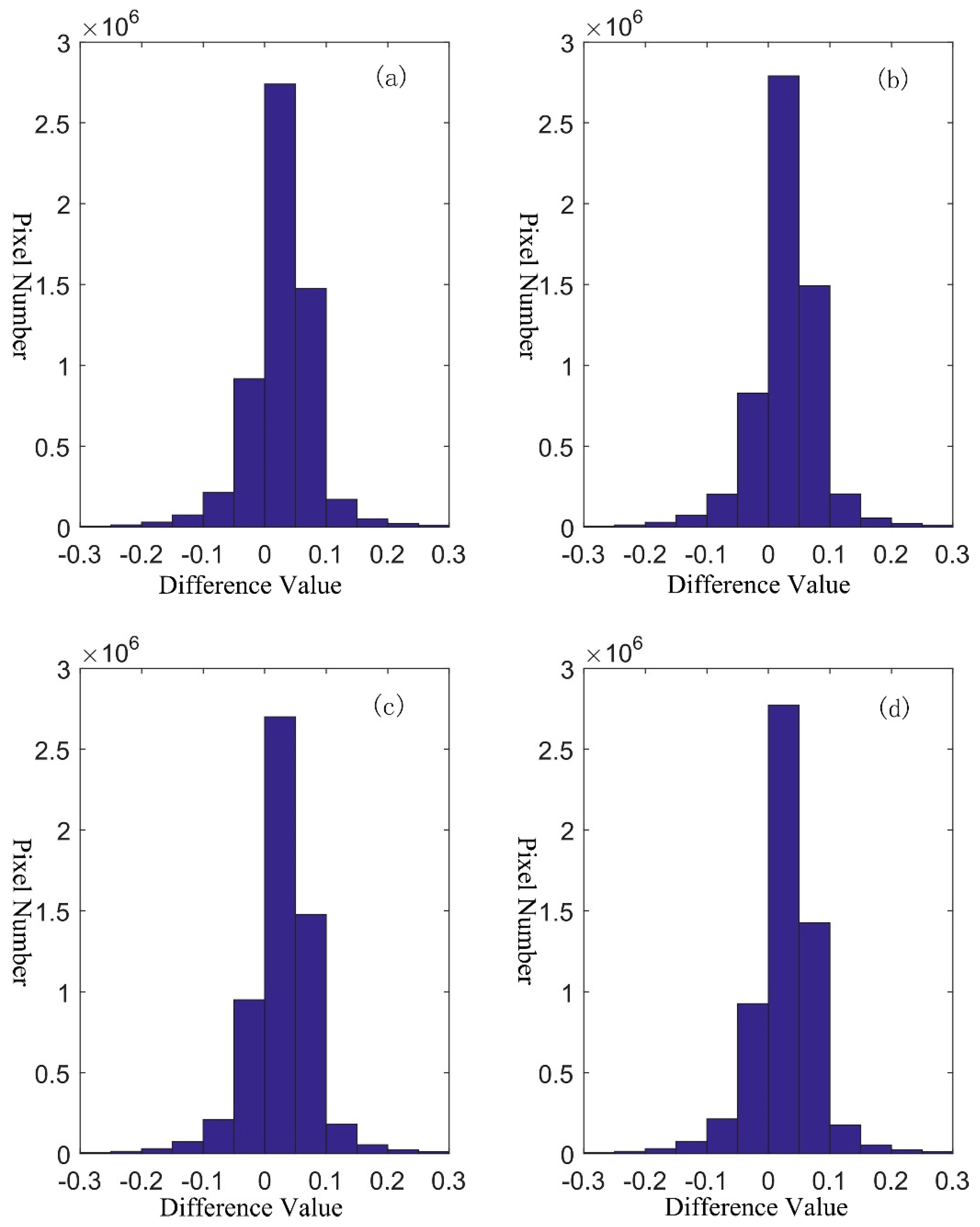
4.4. Temporal–Spatial Comparisons

To assess the spatial performances of these FVC estimation algorithms for VIIRS data, the regional FVC maps (tile H12V09, which was acquired on 29 July 2013) were generated using the four trained machine learning methods (Figure 7) and compared with the corresponding GLASS FVC product. This area is in the Amazon region, located in northern Brazil. The dominant vegetation type in this region is tropical rain forest. Visually, the results show that these estimated FVC maps derived from the four machine learning methods have good spatial agreements compared with the GLASS FVC. Because the FVC estimation algorithm for VIIRS data in this study was developed based on the GLASS FVC product, the spatial consistencies of these FVC maps indicate the reliability of these methods.

To quantify the differences between these FVC estimates and the GLASS FVC product, the GLASS FVC was subtracted by the FVC estimates, and the statistical histograms of the differences are shown in Figure 8. More than 90% of the differences were located between −0.1 and 0.1. The peak values of the statistical histograms were located on zero approximately. These results further indicated that the FVC estimates from the four machine learning methods and GLASS FVC product were consistent and confirmed the reliability of the proposed algorithm.

To analyze the temporal variations of the FVC estimates from the four machine learning methods, the FVC temporal profiles of the Heihe study area in 2012 were generated and compared with the reference FVC data. After spatial matching between the FVC estimated from VIIRS data and the reference FVC data from ASTER and CASI, 144 (12 * 12) pixel values were derived in this study area. The FVC estimates showed satisfactory temporal continuity and one sample pixel was randomly selected from the 144 spatially matched pixels to show the temporal profiles (Figure 9). The representative FVC temporal profiles were consistent with the growth rhythms of maize, which had a primary growing season from May to September. Furthermore, the FVC temporal profiles derived from different machine learning methods also showed good temporal consistencies, and the FVC estimates approached the ASTER/CASI FVC data, which is shown in Figure 9. Therefore, the temporal comparison further confirmed the reliability of the proposed FVC estimation algorithm for VIIRS data.

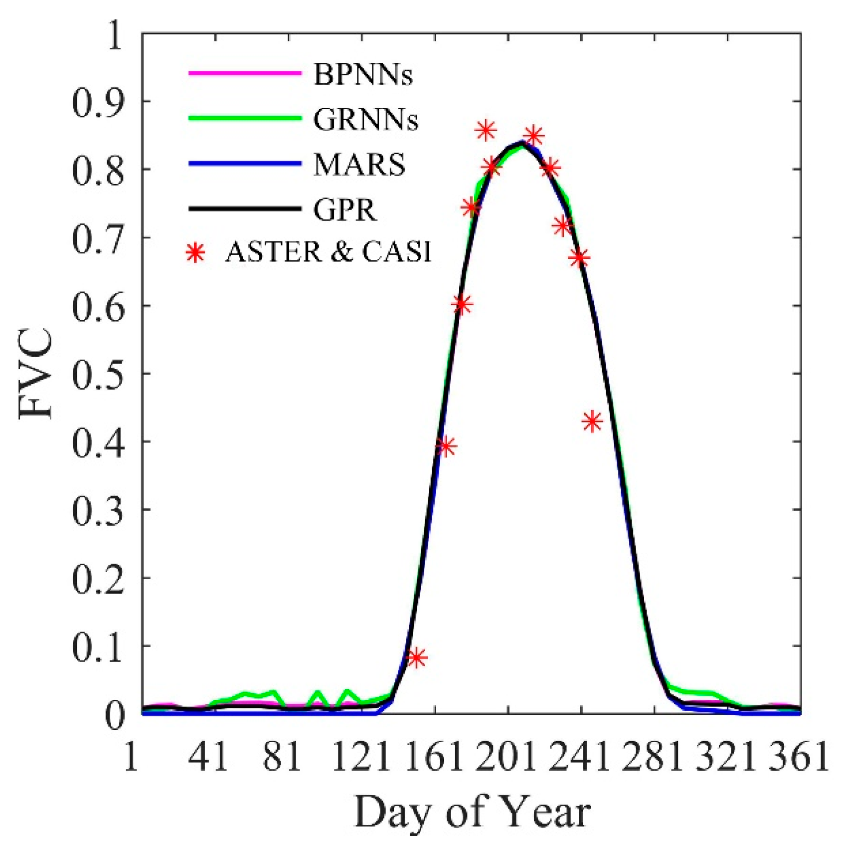
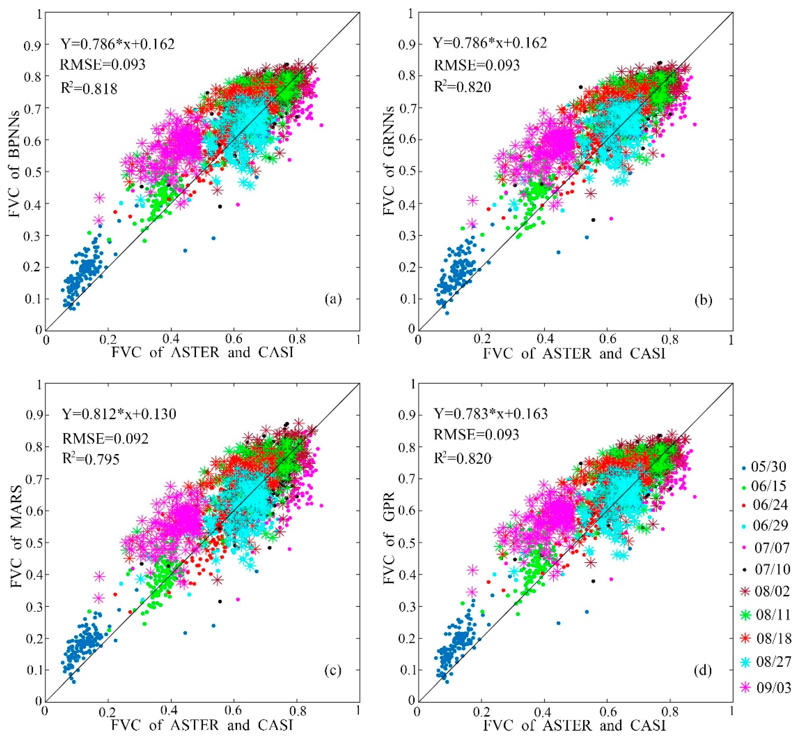
4.5. Direct Accuracy Validation in Heihe Region

The time series FVC estimates in Heihe study area were temporally interpolated using a bilinear interpolation method to obtain the same dates as the ASTER and CASI acquiring dates (Table 1) and the interpolated FVC estimates were compared with the reference FVC data to evaluate the accuracy of the FVC estimates. Scatterplots of the FVC estimates derived from these four machine learning methods and ASTER/CASI FVC data are shown in Figure 10. The results show that the FVC estimates from the four machine learning methods have good linear relationships with the ASTER/CASI FVC data, which approaches the 1:1 line. The overall RMSEs of the four FVC estimates were less than 0.1, and the R² values of the four FVC estimates were larger than 0.75. In addition, some scatter points with moderate FVC values were located above the reference line, which indicated the FVC estimates obtained using the proposed method were slightly higher than ASTER/CASI FVC data. These FVC values were mainly generated on 15 June and 3 September, which were during the maize growth periods with rapid FVC variations that could be seen from the temporal FVC profiles in Figure 9. The main reasons for the deviation might be the uncertainties in the bilinear interpolation of the VIIRS FVC during the rapid maize variation periods and the residual errors in the statistical model while transferring the field FVC measurements to the ASTER/CASI FVC maps. Considering these uncertainties, the slight deviation of the FVC estimated using the proposed method in the rapid FVC variation periods of maize was acceptable. Therefore, the results further indicate that the developed FVC estimation algorithm is robust and effective for FVC estimation based on VIIRS data.

5. Discussion

In this study, a robust global FVC estimation algorithm for VIIRS data was presented. The proposed FVC estimation algorithm for VIIRS data is automatically operated without any priori-knowledge or human interactions. In addition, this algorithm can overcome the difficulties of determining model parameters in empirical models and pixel unmixing models. The algorithm also has advantage in high-efficiency computations, which can be used to operationally estimate long term global FVC from VIIRS data.

Furthermore, the accuracy and representativeness of training samples are essential for the proposed method. The BELMANIP network, which was used in this study, ensured that the training samples contained the most vegetation types on the land surface. Meanwhile, the VIIRS reflectance data were reconstructed using the VIRR method to generate high-quality reflectance data, and the training samples were further refined. Also, the training samples were extracted from the entire year of 2013, which contained the growing seasons for most vegetation and the training sample quality was sufficient. With the high-quality and representative sample data, the algorithm proposed in this study had potential for global FVC estimation with both temporal and spatial continuities. Two test areas were used to evaluate the performances of the proposed algorithm, which indicated the proposed algorithm could generate FVC estimates with temporal–spatial continuities and reliable accuracy comparable with the GLASS FVC product.

In the prior studies, the MODIS data were widely used for FVC estimation [27,47]. However, the MODIS sensor has exceeded its design life and the VIIRS sensor as the successor will continue its earth observation mission. Thus, the proposed algorithm, global FVC estimation algorithm for VIIRS data, can solve the continuity of MODIS FVC estimations on the global scale. Meanwhile, the validation of coarse resolution FVC products is still an important issue, because reference data matching the coarse resolution pixels are still rare. Therefore, further study will focus on extensively validating the proposed algorithm on other typical regions, based on collecting more field survey FVC data with less measurement uncertainties.

6. Conclusions

In this study, a robust global FVC estimation algorithm for VIIRS surface reflectance data was proposed, which is based on machine learning methods (BPNNs, GRNNs, MARS and GPR). The validation results indicated that all four machine learning methods had similar and satisfactory performances. From this study, three main conclusions were drawn: (1) The GPR method achieved better FVC estimation accuracy (RMSE = 0.0887, R² = 0.9019) using VIIRS data than the other three machine learning methods. The GPR method could also generate the uncertainties of FVC estimation, which were useful for many data assimilation models using FVC data. (2) The MARS method had advantages for computational efficiency and similar FVC estimation accuracy with the GPR model. (3) The algorithm could generate FVC estimates with good temporal and spatial continuities, which were useful for various applications. Future work will focus on an extensive assessment of the proposed FVC estimation algorithm for VIIRS data using more ground measurements under different conditions.

References

1. Camacho, F.; Cernicharo, J.; Lacaze, R.; Baret, F.; Weiss, M. GEOV1: LAI, FAPAR essential climate variables and FCOVER global time series capitalizing over existing products. Part 2: Validation and intercomparison with reference products. Remote Sens. Environ. 2013, 137, 310–329. [Google Scholar] [CrossRef]
2. Zhang, X.; Liao, C.; Li, J.; Sun, Q. Fractional vegetation cover estimation in arid and semi-arid environments using HJ-1 satellite hyperspectral data. Int. J. Appl. Earth Observ. Geoinform. 2013, 21, 506–512. [Google Scholar] [CrossRef]
3. Jia, K.; Liang, S.; Gu, X.; Baret, F.; Wei, X.; Wang, X.; Yao, Y.; Yang, L.; Li, Y. Fractional vegetation cover estimation algorithm for Chinese GF-1 wide field view data. Remote Sens. Environ. 2016, 177, 184–191. [Google Scholar] [CrossRef]
4. Roujean, J.L.; Lacaze, R. Global mapping of vegetation parameters from POLDER multiangular measurements for studies of surface-atmosphere interactions: A pragmatic method and its validation. J. Geophys. Res. Atmos. 2002. [Google Scholar] [CrossRef]
5. Baret, F.; Pavageau, K.; Béal, D.; Weiss, M.; Barthelot, B.; Regner, P. Algorithm Theoretical Basis Document for MERIS Top of Atmosphere Land Products (TOAVEG); Report of ESA contract AO; The European Space Agency: Paris, France, 2006. [Google Scholar]
6. García-Haro, F.J.; Camacho-de Coca, F.; Miralles, J.M. Inter-comparison of SEVIRI/MSG and MERIS/ENVISAT biophysical products over Europe and Africa. In Proceedings of the 2nd MERIS/(A) ATSR User Workshop, Frascati, Italy, 22–26 September 2008; pp. 22–26. [Google Scholar]
7. Baret, F.; Weiss, M.; Lacaze, R.; Camacho, F.; Makhmara, H.; Pacholcyzk, P.; Smets, B. GEOV1: LAI and FAPAR essential climate variables and FCOVER global time series capitalizing over existing products. Part 1: Principles of development and production. Remote Sens. Environ. 2013, 137, 299–309. [Google Scholar] [CrossRef]
8. Guenther, B.; de Luccia, F.; McCarthy, J.; Moeller, C.; Xiong, X.; Murphy, R.E. Performance continuity of the A-Train MODIS observations: Welcome to the NPP VIIRS. Available online: https://www.star.nesdis.noaa.gov/jpss/documents/meetings/2011/AMS_Seattle_2011/Poster/A-TRAIN%20%20Perf%20Cont%20%20MODIS%20Observa%20-%20Guenther%20-%20WPNB.pdf (accessed on 25 May 2018 ).
9. Xiong, X.; Sun, J.; Barnes, W.; Salomonson, V.; Esposito, J.; Erives, H.; Guenther, B. Multiyear on-orbit calibration and performance of Terra MODIS reflective solar bands. IEEE Trans. Geosci. Remote Sens. 2007, 45, 879–889. [Google Scholar] [CrossRef]
10. Vermote, E.; Justice, C.; Csiszar, I. Early evaluation of the VIIRS calibration, cloud mask and surface reflectance Earth data records. Remote Sens. Environ. 2014, 148, 134–145. [Google Scholar] [CrossRef]
11. Jiao, Z.; Yan, G.; Zhao, J.; Wang, T.; Chen, L. Estimation of surface upward longwave radiation from MODIS and VIIRS clear-sky data in the Tibetan Plateau. Remote Sens. Environ. 2015, 162, 221–237. [Google Scholar] [CrossRef]
12. Meng, F.; Cao, C.; Shao, X. Spatio-temporal variability of Suomi-NPP VIIRS-derived aerosol optical thickness over China in 2013. Remote Sens. Environ. 2015, 163, 61–69. [Google Scholar] [CrossRef]
13. Shabanov, N.; Vargas, M.; Miura, T.; Sei, A.; Danial, A. Evaluation of the performance of Suomi NPP VIIRS top of canopy vegetation indices over AERONET sites. Remote Sens. Environ. 2015, 162, 29–44. [Google Scholar] [CrossRef]
14. Wang, D.; Liang, S.; He, T.; Yu, Y. Direct estimation of land surface albedo from VIIRS data: Algorithm improvement and preliminary validation. J. Geophys. Res. Atmos. 2013. [Google Scholar] [CrossRef]
15. Xiao, Z.; Liang, S.; Wang, T.; Jiang, B. Retrieval of leaf area index (LAI) and fraction of absorbed photosynthetically active radiation (FAPAR) from VIIRS time-series data. Remote Sens. 2016, 8, 351. [Google Scholar] [CrossRef]
16. Xiao, J.; Moody, A. A comparison of methods for estimating fractional green vegetation cover within a desert-to-upland transition zone in central New Mexico, USA. Remote Sens. Environ. 2005, 98, 237–250. [Google Scholar] [CrossRef]
17. Jiapaer, G.; Chen, X.; Bao, A. A comparison of methods for estimating fractional vegetation cover in arid regions. Agric. For. Meteorol. 2011, 151, 1698–1710. [Google Scholar] [CrossRef]
18. Bioucas-Dias, J.M.; Plaza, A.; Dobigeon, N.; Parente, M.; Du, Q.; Gader, P.; Chanussot, J. Hyperspectral unmixing overview: Geometrical, statistical, and sparse regression-based approaches. IEEE J. Sel. Top. Appl. Earth Observ. Remote Sens. 2012, 5, 354–379. [Google Scholar] [CrossRef]
19. Adams, J.B.; Smith, M.O.; Johnson, P.E. Spectral mixture modeling: A new analysis of rock and soil types at the Viking Lander 1 site. J. Geophys. Res. Solid Earth 1986, 91, 8098–8112. [Google Scholar] [CrossRef]
20. Price, J.C. Estimating leaf area index from satellite data. IEEE Trans. Geosci. Remote Sens. 1993, 31, 727–734. [Google Scholar] [CrossRef]
21. Gutman, G.; Ignatov, A. The derivation of the green vegetation fraction from NOAA/AVHRR data for use in numerical weather prediction models. Int. J. Remote Sens. 1998, 19, 1533–1543. [Google Scholar] [CrossRef]
22. Case, J.L.; LaFontaine, F.J.; Bell, J.R.; Jedlovec, G.J.; Kumar, S.V.; Peters-Lidard, C.D. A real-time MODIS vegetation product for land surface and numerical weather prediction models. IEEE Trans. Geosci. Remote Sens. 2014, 52, 1772–1786. [Google Scholar] [CrossRef]
23. Yang, L.; Jia, K.; Liang, S.; Liu, J.; Wang, X. Comparison of four machine learning methods for generating the GLASS fractional vegetation cover product from MODIS data. Remote Sens. 2016, 8, 682. [Google Scholar] [CrossRef]
24. Yang, L.; Jia, K.; Liang, S.; Wei, X.; Yao, Y.; Zhang, X. A Robust Algorithm for Estimating Surface Fractional Vegetation Cover from Landsat Data. Remote Sens. 2017, 9, 857. [Google Scholar] [CrossRef]
25. Verrelst, J.; Muñoz, J.; Alonso, L.; Delegido, J.; Rivera, J.P.; Camps-Valls, G.; Moreno, J. Machine learning regression algorithms for biophysical parameter retrieval: Opportunities for Sentinel-2 and-3. Remote Sens. Environ. 2012, 118, 127–139. [Google Scholar] [CrossRef]
26. Ahmad, S.; Kalra, A.; Stephen, H. Estimating soil moisture using remote sensing data: A machine learning approach. Adv. Water Resour. 2010, 33, 69–80. [Google Scholar] [CrossRef]
27. Jia, K.; Liang, S.; Liu, S.; Li, Y.; Xiao, Z.; Yao, Y.; Jiang, B.; Zhao, X.; Wang, X.; Xu, S.; et al. Global land surface fractional vegetation cover estimation using general regression neural networks from MODIS surface reflectance. IEEE Trans. Geosci. Remote Sens. 2015, 53, 4787–4796. [Google Scholar] [CrossRef]
28. Pasolli, L.; Melgani, F.; Blanzieri, E. Gaussian process regression for estimating chlorophyll concentration in subsurface waters from remote sensing data. IEEE Geosci. Remote Sens. Lett. 2010, 7, 464–468. [Google Scholar] [CrossRef]
29. Baret, F.; Morissette, J.T.; Fernandes, R.A.; Champeaux, J.L.; Myneni, R.B.; Chen, J.; Plummer, S.; Weiss, M.; Bacour, C.; Garrigues, S.; et al. Evaluation of the representativeness of networks of sites for the global validation and intercomparison of land biophysical products: Proposition of the CEOS-BELMANIP. IEEE Trans. Geosci. Remote Sens. 2006, 44, 1794–1803. [Google Scholar] [CrossRef]
30. Olson, D.M.; Dinerstein, E.; Wikramanayake, E.D.; Burgess, N.D.; Powell, G.V.; Underwood, E.C.; D’amico, J.A.; Itoua, I.; Strand, H.E.; Morrison, J.C.; et al. Terrestrial Ecoregions of the World: A New Map of Life on Earth: A new global map of terrestrial ecoregions provides an innovative tool for conserving biodiversity. BioScience 2001, 51, 933–938. [Google Scholar] [CrossRef]
31. Zhang, R.; Huang, C.; Zhan, X.; Dai, Q.; Song, K. Development and validation of the global surface type data product from S-NPP VIIRS. Remote Sens. Lett. 2016, 7, 51–60. [Google Scholar] [CrossRef]
32. Gitelson, A.A.; Kaufman, Y.J.; Stark, R.; Rundquist, D. Novel algorithms for remote estimation of vegetation fraction. Remote Sens.Environ. 2002, 80, 76–87. [Google Scholar] [CrossRef] [Green Version]
33. Xiao, Z.; Liang, S.; Wang, T.; Liu, Q. Reconstruction of satellite-retrieved land-surface reflectance based on temporally-continuous vegetation indices. Remote Sens. 2015, 7, 9844–9864. [Google Scholar] [CrossRef]
34. Garcia, D. Robust smoothing of gridded data in one and higher dimensions with missing values. Comput. Stat. Data Anal. 2010, 54, 1167–1178. [Google Scholar] [CrossRef] [PubMed] [Green Version]
35. Liang, S.; Zhang, X.; Xiao, Z.; Cheng, J.; Liu, Q.; Zhao, X. Global LAnd Surface Satellite (GLASS) Products: Algorithms, Validation and Analysis; Springer Science & Business Media: Berlin, Germany, 2013. [Google Scholar]
36. Liang, S.; Zhao, X.; Liu, S.; Yuan, W.; Cheng, X.; Xiao, Z.; Zhang, X.; Liu, Q.; Cheng, J.; Tang, H.; et al. A long-term Global LAnd Surface Satellite (GLASS) data-set for environmental studies. Int. J. Dig. Earth 2013, 6, 5–33. [Google Scholar] [CrossRef] [Green Version]
37. Mu, X.; Huang, S.; Ren, H.; Yan, G.; Song, W.; Ruan, G. Validating GEOV1 fractional vegetation cover derived from coarse-resolution remote sensing images over croplands. IEEE J. Sel. Top. Appl. Earth Observ. Remote Sens. 2015, 8, 439–446. [Google Scholar] [CrossRef]
38. Liu, Y.; Mu, X.; Wang, H.; Yan, G. A novel method for extracting green fractional vegetation cover from digital images. J. Veg. Sci. 2012, 23, 406–418. [Google Scholar] [CrossRef]
39. Song, W.; Mu, X.; Yan, G.; Huang, S. Extracting the green fractional vegetation cover from digital images using a shadow-resistant algorithm (SHAR-LABFVC). Remote Sens. 2015, 7, 10425–10443. [Google Scholar] [CrossRef]
40. Chen, J.; Liao, A.; Chen, J.; Peng, S.; Chen, L.; Zhang, H. 30-m Global Land cover data product-Globe Land30. Geomatics World 2017, 24, 1–8. (In Chinese) [Google Scholar] [CrossRef]
41. Wang, X.; Jia, K.; Liang, S.; Zhang, Y. Fractional Vegetation Cover Estimation Method Through Dynamic Bayesian Network Combining Radiative Transfer Model and Crop Growth Model. IEEE Trans. Geosci. Remote Sens. 2016, 54, 7442–7450. [Google Scholar] [CrossRef]
42. Baret, F.; Hagolle, O.; Geiger, B.; Bicheron, P.; Miras, B.; Huc, M.; Berthelot, B.; Niño, F.; Weiss, M.; Samain, O.; et al. LAI, fAPAR and fCover CYCLOPES global products derived from VEGETATION: Part 1: Principles of the algorithm. Remote Sens. Environ. 2007, 110, 275–286. [Google Scholar] [CrossRef] [Green Version]
43. Kavzoglu, T.; Mather, P.M. The use of backpropagating artificial neural networks in land cover classification. Int. J. Remote Sens. 2003, 24, 4907–4938. [Google Scholar] [CrossRef]
44. Specht, D.F. A general regression neural network. IEEE Trans. Neural Netw. 1991, 2, 568–576. [Google Scholar] [CrossRef] [PubMed]
45. Friedman, J.H. Multivariate adaptive regression splines. Ann. Stat. 1991, 19, 1–67. [Google Scholar] [CrossRef]
46. Lee, T.-S.; Chen, I.-F. A two-stage hybrid credit scoring model using artificial neural networks and multivariate adaptive regression splines. Expert Syst. Appl. 2005, 28, 743–752. [Google Scholar] [CrossRef]
47. Rasmussen, C.E.; Williams, C.K. Gaussian Processes for Machine Learning; MIT Press: Cambridge, MA, USA, 2006; Volume 1. [Google Scholar]
Figure 1. Global sample locations from the Benchmark Land Multisite Analysis and Intercomparison of Products (BELMANIP) network.
Remotesensing 10 01648 g001
Figure 2. The location and main land types of the study area (Left: 30-m resolution land cover distributions from the Global Land Cover Product [40]. Right: false color image of the Advanced Spaceborne Thermal Emission and Reflection Radiometer (ASTER) data on 30 May 2012 [37]).
Remotesensing 10 01648 g002
Figure 3. Global fractional vegetation cover (FVC) estimation algorithm flowchart for Visible Infrared Imaging Radiometer Suite (VIIRS) surface reflectance data.
Remotesensing 10 01648 g003
Figure 4. The VIIRS surface reflectances of the red and NIR bands as well as the NDVI before and after reconstructions at the Maun, Floodplain site (Lat: −19.66°, Lon: 23.35°) in 2013.
Remotesensing 10 01648 g004
Figure 5. The VIIRS surface reflectance of the red and NIR bands as well as NDVI before and after reconstructions at ARM/CART Shilder site (Lat: 36.93°, Lon: −96.86°) in 2013.
Remotesensing 10 01648 g005
Figure 6. Density scatter plots of the NDVI from VIIRS data and the Global LAnd Surface Satellite (GLASS) FVC values for the refined training samples.
Remotesensing 10 01648 g006
Figure 7. The false color map of the VIIRS data and FVC maps derived from the four machine learning methods, as well as GLASS FVC product: (a) False color map of VIIRS reflectance data (R, G and B channels with VIIRS reflectance of NIR, Red and short-wave infrared (SWIR) bands, respectively); (b) back propagating neural networks (BPNNs); (c) general regression networks (GRNNs); (d) MARS; (e) Gaussian process regression (GPR) and (f) GLASS FVC.
Remotesensing 10 01648 g007
Figure 8. Histograms of differences between the FVC estimated from the four machine learning methods and the GLASS FVC: (a) BPNNs; (b) GRNNs; (c) MARS; and (d) GPR.
Remotesensing 10 01648 g008
Figure 9. FVC temporal profiles derived from the VIIRS data using the four machine learning methods and the ASTER/CASI FVC data from Heihe in 2012.
Remotesensing 10 01648 g009
Figure 10. Scatterplots of comparison results of FVC estimates from the four methods and the ASTER/CASI FVC data: (a) BPNNs; (b) GRNNs; (c) MARS; (d) GPR.
Remotesensing 10 01648 g010