Guidelines for Underwater Image Enhancement Based on Benchmarking of Different Methods
by
 , , and
Marino Mangeruga
1,2 ,
,
Fabio Bruno
1,2,* ,
,
Marco Cozza
2,
Panagiotis Agrafiotis
3 and
Dimitrios Skarlatos
3 1
University of Calabria, Rende, 87036 Cosenza, Italy
2
3D Research s.r.l., Rende, 87036 Cosenza, Italy
3
Photogrammetric Vision Laboratory, Department of Civil Engineering and Geomatics, Cyprus University of Technology, 3036 Limassol, Cyprus
*
Author to whom correspondence should be addressed.
Remote Sens. 2018, 10(10), 1652; https://0-doi-org.brum.beds.ac.uk/10.3390/rs10101652
Submission received: 11 September 2018
/
Revised: 7 October 2018
/
Accepted: 12 October 2018
/
Published: 17 October 2018
(This article belongs to the Section Remote Sensing Image Processing)
Abstract
:Images obtained in an underwater environment are often affected by colour casting and suffer from poor visibility and lack of contrast. In the literature, there are many enhancement algorithms that improve different aspects of the underwater imagery. Each paper, when presenting a new algorithm or method, usually compares the proposed technique with some alternatives present in the current state of the art. There are no studies on the reliability of benchmarking methods, as the comparisons are based on various subjective and objective metrics. This paper would pave the way towards the definition of an effective methodology for the performance evaluation of the underwater image enhancement techniques. Moreover, this work could orientate the underwater community towards choosing which method can lead to the best results for a given task in different underwater conditions. In particular, we selected five well-known methods from the state of the art and used them to enhance a dataset of images produced in various underwater sites with different conditions of depth, turbidity, and lighting. These enhanced images were evaluated by means of three different approaches: objective metrics often adopted in the related literature, a panel of experts in the underwater field, and an evaluation based on the results of 3D reconstructions.

1. Introduction
The scattering and absorption of light causes the quality degradation of underwater images. These phenomena are caused by suspended particles in water and by the propagation of light through the water, which is attenuated differently according to its wavelength, water column depth, and the distance between the objects and the point of view. Consequently, as the water column increases, the various components of sunlight are differently absorbed by the medium, depending on their wavelengths. This leads to a dominance of blue/green colours in underwater imagery, which is known as colour cast. The employment of artificial light can increase the visibility and recover the colour, but an artificial light source does not illuminate the scene uniformly and can produce bright spots in the images due to the backscattering of light in the water medium.
The benchmark presented in this research is a part of the iMARECULTURE project [1,2,3], which aims to develop new tools and technologies to improve the public awareness of underwater cultural heritage. In particular, it includes the development of a Virtual Reality environment that reproduces faithfully the appearance of underwater sites, thus offering the possibility to visualize the archaeological remains as they would appear in air. This goal requires the benchmarking of different image enhancement methods to figure out which one performs better in different environmental and illumination conditions. We published another work [4] in which we selected five methods from the state of the art and used them to enhance a dataset of images produced in various underwater sites at heterogeneous conditions of depth, turbidity and lighting. These enhanced images were evaluated by means of some quantitative metrics. Presently, we will extend our previous work by introducing two more approaches meant for a more comprehensive benchmarking of the underwater image enhancement methods. The first of these additional approaches was conducted with a panel of experts in the field of underwater imagery, members of iMARECULTURE project, and the other one is based on the results of 3D reconstructions. Furthermore, since we modified some images in our dataset by adding some new ones, we also report the results of the quantitative metrics, as done in our previous work.
In highly detailed underwater surveys, the availability of radiometric information, along with 3D data regarding the surveyed objects, becomes crucial for many diagnostics and interpretation tasks [5]. To this end, different image enhancement and colour correction methods have been proposed and tested for their effectiveness in both clear and turbid waters [6]. Our purpose was to supply the researchers in the underwater community with more detailed information about the employment of a specific enhancement method in different underwater conditions. Moreover, we were interested in verifying whether different benchmarking approaches have produced consistent results.
The problem of underwater image enhancement is closely related to single image dehazing, in which images are degraded by weather conditions such as haze or fog. A variety of approaches have been proposed to solve image dehazing, and in the present paper we have reported their most effective examples. Furthermore, we also report methods that address the problem of non-uniform illumination in the images and those that focus on colour correction.
Single image dehazing methods assume that only one input image is available and rely on image priors to recover a dehazed scene. One of the most cited works on single image dehazing is the dark channel prior (DCP) [7]. It assumes that, within small image patches, there will be at least one pixel with a dark colour channel. It then uses this assumption to estimate the transmission and to recover the image. However, this prior was not designed to work underwater, and it does not take into account the different absorption rates of the three colour channels. In [8], an extension of DCP to deal with underwater image restoration is presented. Given that the red channel is often nearly dark in underwater images, this new prior called Underwater Dark Channel Prior (UDCP) considers just the green and the blue colour channels in order to estimate the transmission. An author mentioned many times in the field is Fattal, R and his two works [9,10]. In the first work [9], Fattal et al., taking into account surface shading and the transmission function, tried to resolve ambiguities in data by searching for a solution in which the resulting shading and transmission functions are statistically uncorrelated.
The second work [10] describes a new method based on a generic regularity in natural images, which is referred to as colour-lines. On this basis, Fattal et al. derived a local formation model that explains the colour-lines in the context of hazy scenes and used it to recover the image. Another work focused on lines of colour is presented in [11,12]. The authors describe a new prior for single image dehazing that is defined as a Non-Local prior, to underline that the pixels forming the lines of colour are spread across the entire image, thus capturing a global characteristic that is not limited to small image patches.
Some other works focus on the problem of non-uniform illumination that, in the case of underwater imagery, is often produced by an artificial light in deep water. The work proposed in [13] assumes that natural underwater images are Rayleigh distributed and uses maximum likelihood estimation of scale parameters to map distribution of image to Rayleigh distribution. Next, Morel et al. [14] presents a simple gradient domain method that acts as a high-pass filter, trying to correct the illumination without affecting the image details. A simple prior which estimates the depth map of the scene considering the difference in attenuation among the different colour channels is proposed in [15]. The scene radiance is recovered from a hazy image through an estimated depth map by modelling the true scene radiance as a Markov Random Field.
Bianco et al. presented, in [16], the first proposal for the colour correction of underwater images by using lαβ colour space. A white balancing is performed by moving the distributions of the chromatic components (α, β) around the white point and the image contrast is improved through a histogram cut-off and stretching of the luminance (l) component. More recently, in [17], a fast enhancement method for non-uniformly illuminated underwater images is presented. The method is based on a grey-world assumption applied in the Ruderman-lab opponent colour space. The colour correction is performed according to locally changing luminance and chrominance by using the summed-area table technique. Due to the low complexity cost, this method is suitable for real-time applications, ensuring realistic colours of the objects, more visible details and enhanced visual quality. Works [18,19] present a method of unsupervised colour correction for general purpose images. It employs a computational model that is inspired by some adaptation mechanisms of the human vision to realize a local filtering effect by taking into account the colour spatial distribution in the image.
Additionally, we report a method for contrast enhancement, since underwater images are often lacking in contrast. This is the Contrast Limited Adaptive Histogram Equalization (CLAHE) proposed in [20] and summarized in [21], which was originally developed for medical imaging and has proven to be successful for enhancing low-contrast images.
In [22], a fusion-based underwater image enhancement technique using contrast stretching and Auto White Balance is presented. In [23], a dehazing approach that builds on an original colour transfer strategy to align the colour statistics of a hazy input to the ones of a reference image, also captured underwater, but with neglectable water attenuation, is delivered. There, the colour-transferred input is restored by inverting a simplified version of the McGlamery underwater image formation model, using the conventional Dark Channel Prior (DCP) to estimate the transmission map and the backscattered light parameter involved in the model.
Work [24] proposes a Red Channel method in order to restore the colours of underwater images. The colours associated with short wavelengths are recovered, leading to a recovery of the lost contrast. According to the authors, this Red Channel method can be interpreted as a variant of the DCP method used for images degraded by the atmosphere when exposed to haze. Experimental results show that the proposed technique handles artificially illuminated areas gracefully, and achieves a natural colour correction and superior or equivalent visibility improvement when compared to other state-of-the-art methods. However, it is suitable either for shallow waters, where the red colour still exists, or for images with artificial illumination. The authors in [25] propose a modification to the well-known DCP method. Experiments on real-life data show that this method outperforms competing solutions based on the DCP. Another method that relies in part on the DCP method is presented in [26], where an underwater image restoration method is presented based on transferring an underwater style image into a recovered style using Multi-Scale Cycle Generative Adversarial Network System. There, a Structural Similarity Index Measure loss is used to improve underwater image quality. Then, the transmission map is fed into the network for multi-scale calculation on the images, which combine the DCP method and Cycle-Consistent Adversarial Networks. The work presented in [27] describes a restoration method that compensates for the colour loss due to the scene-to-camera distance of non-water regions without altering the colour of pixels representing water. This restoration is achieved without prior knowledge of the scene depth.
In [28], a deep learning approach is adopted; a Convolutional Neural Network-based image enhancement model is trained efficiently using a synthetic underwater image database. The model directly reconstructs the clear latent underwater image by leveraging on an automatic end-to-end and data-driven training mechanism. Experiments performed on synthetic and real-world images indicate a robust and effective performance of the proposed method.
In [29], exposure bracketing imaging is used to enhance the underwater image by fusing an image that includes sufficient spectral information of underwater scenes. The fused image allows authors to extract reliable grey information from scenes. Even though this method gives realistic results, it seems to be limited in no real-time applications due to the exposure bracketing process.
In the literature, very few attempts at underwater image enhancement methods evaluation through feature matching have been reported, while even fewer of them focus on evaluating the results of 3D reconstruction using the initial and enhanced imagery. Recently, a single underwater image restoration framework based on the depth estimation and the transmission compensation was presented [30]. The proposed scheme consists of five major phases: background light estimation, submerged dark channel prior, transmission refinement and radiance recovery, point spread function deconvolution and transmission and colour compensation. The authors used a wide variety of underwater images with various scenarios in order to assess the restoration performance of the proposed method. In addition, potential applications regarding autopilot and three-dimensional visualization were demonstrated.
Ancuti et al., in [31], as well as in [32], where an updated version of the method is presented, delivered a novel strategy to enhance underwater videos and images built on the fusion principles. There, the utility of the proposed enhancing technique is evaluated through matching by employing the SIFT [33] operator for an initial pair of underwater images, and also for the restored versions of the images. In [34,35], the authors investigated the problem of enhancing the radiometric quality of underwater images, especially in cases where this imagery is going to be used for automated photogrammetric and computer vision algorithms later. There, the initial and the enhanced imagery were used to produce point clouds, meshes and orthoimages, which in turn were compared and evaluated, revealing valuable results regarding the tested image enhancement methods. Finally, in [36], the major challenge of caustics is addressed by a new approach for caustics removal [37]. There, in order to investigate its performance and its effect on the SfM-MVS (Structure from Motion—Multi View Stereo) and 3D reconstruction results, a commercial software performing SfM-MVS was used, the Agisoft’s Photoscan [38] as well as other key point descriptors such as SIFT [33] and SURF [39]. In the tests performed using the Agisoft’s Photoscan, an image pair of the five different datasets was inserted and the alignment step was performed. Regarding the key point detection and matching, using the in-house implementations, a standard detection and matching procedure was followed, using the same image pairs and filtering the initial matches using the RANSAC [40] algorithm and the fundamental matrix. Subsequently, all datasets were used in order to create 3D point clouds. The resulting point clouds were evaluated in terms of total number of points and roughness, a metric that also indicates the noise on the point cloud.
2. A Software Tool for Enhancing Underwater Images
We developed software useful for automatically processing a dataset of underwater images with a set of image enhancement algorithms, and we employed it to simplify the benchmarking of these algorithms. This software implements five algorithms (ACE, CLAHE, LAB, NLD and SP) that perform well and employ different approaches for the resolution of the underwater image enhancement problem, such as image dehazing, non-uniform illumination correction and colour correction.
The decision to select certain algorithms among all the others is based on a brief preliminary evaluation of their enhancement performance. There are numerous methods of underwater image enhancement, and we considered the vast majority of them. Unfortunately, many authors do not release the implementation of their algorithms. An implementation that relies only on what authors described in their papers does not guarantee the accuracy of the enhancement process and can mislead the evaluation of an algorithm. Consequently, we selected those algorithms for which we could find a trustworthy implementation performed by the authors of the papers or by a reliable author. Within these algorithms, we conducted our preliminary evaluation, in order to select the ones that seemed to perform better in different underwater conditions.
The source codes of the five selected algorithms were adapted and merged in our software tool. We employed the OpenCV [41] library for tool development in order to exploit its functions for image managing and processing.
Selected Algorithms and Their Implementation
The selected algorithms are the same ones we used in [4]; consequently, please refer to the paper in question for detailed information. Here, we shall report only a brief description of those algorithms.
The first is the Automatic Colour Enhancement (ACE) algorithm, a very complex technique that we employed using a faster version described in [19]. Two parameters that can be adjusted to tune the algorithm behaviour are α and the weighting function ω(x,y). The α parameter specifies the strength of the enhancement: the larger this parameter, the stronger the enhancement. In our test, we used the standard values for these parameters, e.g., α = 5 and ω(x,y) = 1/‖x − y‖. For the implementation, we used the ANSI C source code with reference to [19], which we adapted in our enhancement tool.
The CLAHE [20,21] algorithm is an improved version of AHE, or Adaptive Histogram Equalization. Both are aimed at improving the standard histogram equalization. CLAHE was designed to prevent the over-amplification of noise that can be generated using the adaptive histogram equalization. We implemented this algorithm in our enhancement tool by employing the CLAHE function provided by the OpenCV library. Two parameters are provided in order to control the output of this algorithm: the tile size and the contrast limit. In our test, we set the tile size at 8 × 8 pixels and the contrast limit to 2.
Another method [16], which we refer to as LAB, is based on the assumptions of grey world and uniform illumination of the scene. The idea behind this method is to convert the input image from RGB to LAB space, correct colour casts of an image by adjusting the α and β components, increasing contrast by performing histogram cut-off and stretching and then convert the image back to the RGB space. The MATLAB implementation provided by the author was very time-consuming; therefore, we managed to port the code to C++ by employing OpenCV, among other libraries. This enabled us to include this algorithm in our enhancement tool, and to decrease the computing time by an order of magnitude.
Berman et al. elaborated a Non-Local Image Dehazing (NLD) method based on the assumption that colours of a haze-free image can be well approximated by a few hundred distinct colours. They conceived the concept of haze lines, by which the algorithm recovers both the distance map and the dehazed image. The algorithm takes linear time with respect to the number of pixels of the image. The authors have published the MATLAB source code that implements their method [11], and in order to include this algorithm in our enhancement tool, we conducted a porting to C++, employing different libraries, such as OpenCV, Eigen [42] for the operation on sparse matrices not supported by OpenCV, and FLANN [43] (Fast Library for Approximate Nearest Neighbours), to compute the colour cluster.
The last algorithm is the Screened Poisson Equation for Image Contrast Enhancement (SP). Its output is an image which is a result of applying the Screened Poisson equation [14] to each colour channel separately, together with the simplest colour balance [44] with a variable percentage of saturation as parameter(s). The ANSI C source code is provided by the authors in [14], and we adapted it in our enhancement tool. For the Fourier transform, this code relies on the library FFTw [45]. The algorithm output can be controlled with the trade-off parameter α and the level of saturation of the simplest colour balance s. In our evaluation, we used α = 0.0001 and s = 0.2 as parameters.
Table 1 shows the running times of these different algorithms on a sample image of 4000 × 3000 pixels. These times were estimated by the means of our software tool on a machine with an i7-920 @ 2.67 GHz processor.
3. Case Studies
We assembled a heterogeneous dataset of images that can represent the variability of environmental and illumination conditions that characterizes underwater imagery. We selected images taken with different cameras and with different resolutions, considering that—when applied in the real world—the underwater image enhancement methods have to deal with images produced by unspecific sources. In this section, we briefly describe the underwater sites and the dataset of images.
3.1. Underwater Sites
Four different sites were selected on which the images for the benchmarking of the underwater image enhancement algorithms were taken. The selected sites are representative of different states of environmental and geomorphologic conditions (i.e., water depth, water turbidity, etc.). Two of them are pilot sites of the iMARECULTURE project: the Underwater Archaeological Park of Baiae, and the Mazotos shipwreck. The other two are the Cala Cicala and Cala Minnola shipwrecks. For detailed information about these underwater sites, please refer to our preceding work [4].
The Underwater Archaeological Park of Baiae is usually characterized by very poor visibility caused by the water turbidity, which in turn is mainly due to the organic particles suspended in the medium. Consequently, the underwater images produced here are strongly affected by the haze effect [46].
The second site is the Mazotos shipwreck, which lies at a depth of 44 m. The visibility in this site is very good, but the red absorption at this depth is nearly total. In our previous work, the images for this site were taken only with artificial light. Now we are considering images taken both with natural light and with an artificial light for recovery of the colour.
The so-called Cala Cicala shipwreck lies at a depth of 5 m, within the Marine Protected Area of Capo Rizzuto (Province of Crotone, Italy). The visibility at this site is good.
Lastly, the underwater archaeological site of Cala Minnola preserves the wreck of a Roman cargo ship at a depth from the sea level ranging from 25 m to 30 m [47]. At this site, the visibility is good, but, due to the water depth, the images taken here suffer from serious colour cast because of the red channel absorption; therefore, they appear bluish.
3.2. Image Dataset
We selected three representative images for each underwater site described in the previous section, except for Mazotos for which we selected three images with natural light and three with artificial light, for a total of fifteen images. These images constitute the underwater dataset that we employed to complete our benchmarking of image enhancement methods.
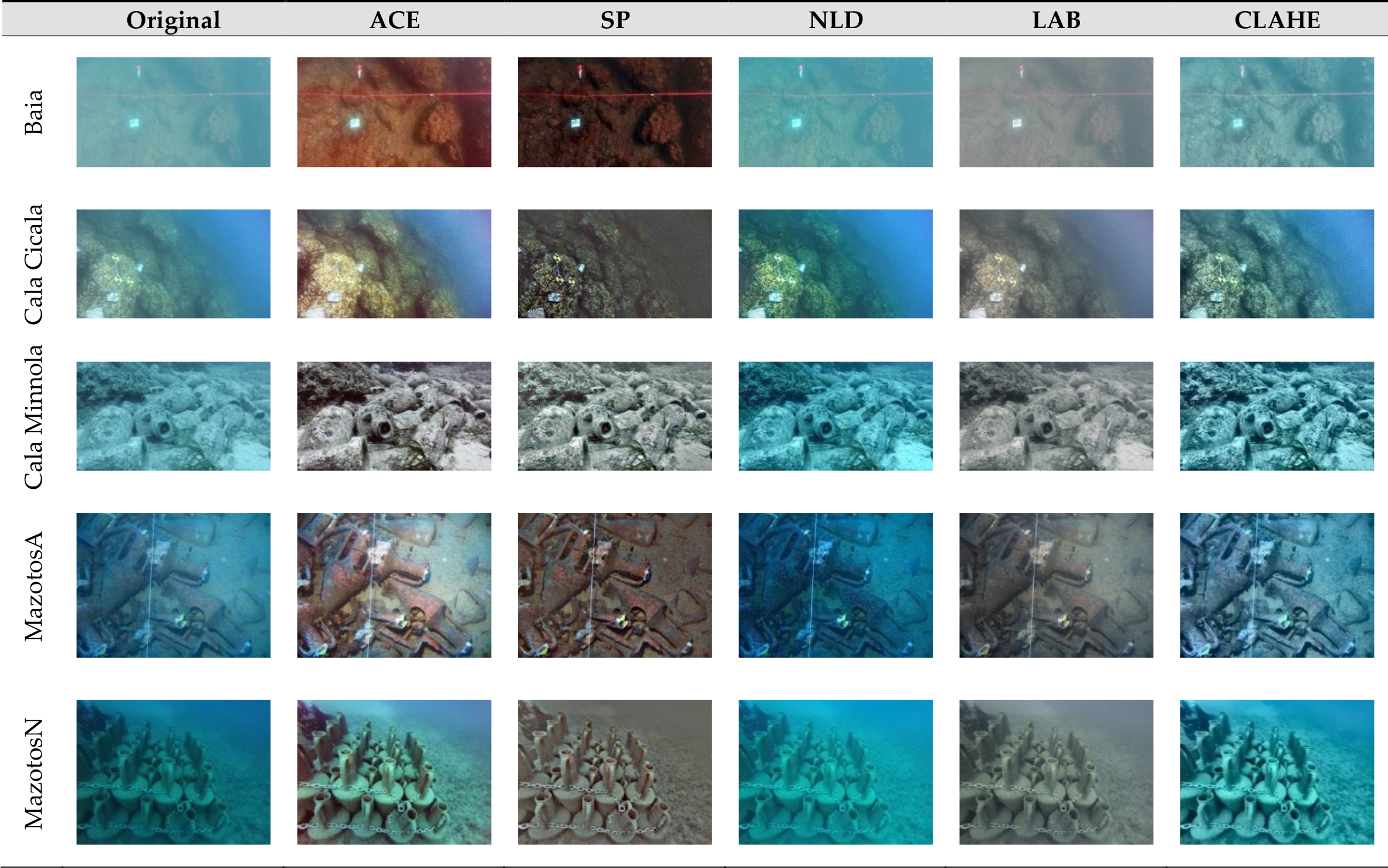
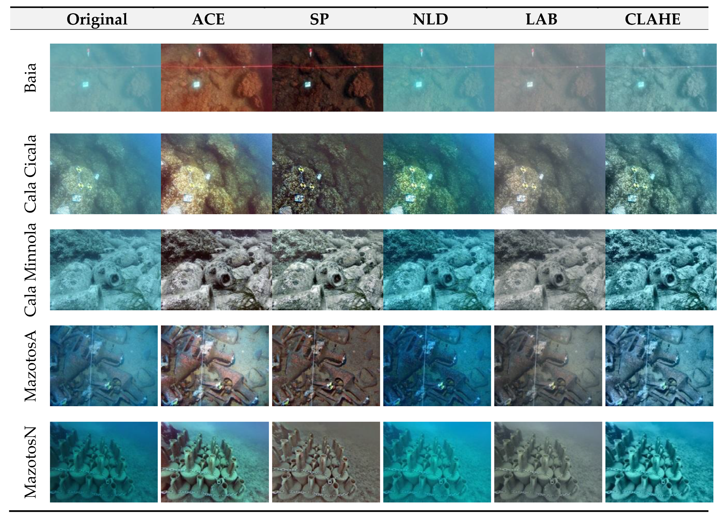
Each row of the Figure 1 represents an underwater site. The properties and modality of acquisition of the images vary depending on the underwater site. The first three rows (a–i) show, respectively, the images acquired in the Underwater Archaeological Park of Baiae, within the Cala Cicala shipwreck, and among the underwater site of Cala Minnola. For additional information about these images, please can refer to our previous work [4].
In the last two rows (j–o), we find the pictures of the amphorae at the Mazotos shipwreck. These images are different from those we employed in our previous work. Due to the considerable water depth, the first three images (j–l) were acquired with an artificial light, which produced a bright spot due to the backward scattering. The last three images were taken with natural light; therefore, they are affected by serious colour cast. Images (j,k) were acquired using a Nikon D90 with a resolution of 4288 × 2848 pixels, (l,n,o) were taken using a Canon EOS 7D with a resolution of 5184 × 3456 pixels, and image (m) was acquired with a Garmin VIRBXE, an action camera, with a resolution of 4000 × 3000 pixels.
The described dataset is composed by very heterogeneous images that address a wide range of potential underwater environmental conditions and problems, as the turbidity in the water that makes the underwater images hazy, the water depth that causes colour casting and the use of artificial light that can lead to bright spots. It makes sense to expect that each of the selected image enhancement methods should perform better on the images that represent the environmental conditions against which it was designed.
4. Benchmarking Based on Objective Metrics
4.1. Evaluation Methods
Each image included in the dataset described in the previous section was processed with each of the image enhancement algorithms previously introduced, taking advantage of the enhancement processing tool that we developed including all the selected algorithms in order to speed up the processing task. The authors suggested some standard parameters for their algorithms in order to obtain good enhancing results. Some of these parameters could be tuned differently in various underwater conditions in order to improve the result. We decided to let all the parameters have the standard values in order not to influence our evaluation with a tuning of the parameters that could have been more effective for one algorithm than for another.
We employed some quantitative metrics, representative of a wide range of metrics employed in the field of underwater image enhancement, to evaluate all the enhanced images. In particular, these metrics are employed in the evaluation of hazy images in [48]. Similar metrics are defined in [49] and employed in [13]. Consequently, the objective performance of the selected algorithms is evaluated in terms of the following metrics. The first one is obtained by calculating the mean value of image brightness (). When is smaller, the efficiency of image dehazing is better. The mean value on the three colour channels () is a simple arithmetic mean. Another metric is the information entropy () that represent the amount of information contained in the image. The bigger the entropy, the better the enhanced image. The mean value () on the three colour channels is defined as a root mean square. The third metric is the average gradient of the image (), which represents a local variance among the pixels of the image; therefore, a larger value indicates a better resolution of the image. The mean value on the three colour channels is a simple arithmetic mean. A more detailed description of these metrics can be found in [4].
4.2. Results
This section reports the results of the objective evaluation performed on all the images in the dataset, both for the original ones and for the ones enhanced with each of the previously described algorithms. The dataset consists of 15 images. Each image has been enhanced by means of the five algorithms; therefore, the total amount of images to be evaluated with the quantitative metrics is 90 (15 originals and 75 enhanced). For practical reasons, we will report here only a sample of our results, i.e., a mosaic composed of the original image named as “MazotosN4” and its five enhanced versions (Figure 2).
Table 2 presents the results of the benchmarking performed through the selected metrics on the images showed in Figure 2. The first column reports the metric values for the original images, and the following columns report the correspondent values for the images enhanced with the concerning algorithms. Each row, on the other hand, reports the value of each metric calculated for each colour channel and its mean value, as previously defined. The values marked in bold correspond to the best value for the metric defined by the corresponding row. By analysing the mean values of the metrics (), it can be deduced that the ACE algorithm performed better on enhancing the information entropy and the SP algorithm performed better on the average gradient.
Focusing on the value of the metric (), we can notice that all the algorithms failed to improve the mean brightness parameter. Looking further into the results and analysing the mean brightness of the single colour channels, we can recognise that its values are very low on the red channel. The validity of the mean brightness metric is based on the assumption that an underwater image is a hazy image and, consequently, a good dehazing leads to a reduced mean brightness. However, this assumption cannot hold in deep water, where the imagery is often non-hazy, but with a heavy red channel adsorption. Therefore, further brightness reducing of this channel in such a situation cannot be considered a valuable result. This is exactly the case of the “MazotosN4” image where the metric was misled, considering that the original image is better than the others. We decided to report this case in order to underline the inadequacy of the mean brightness metric for evaluating images taken in deep water with natural illumination.
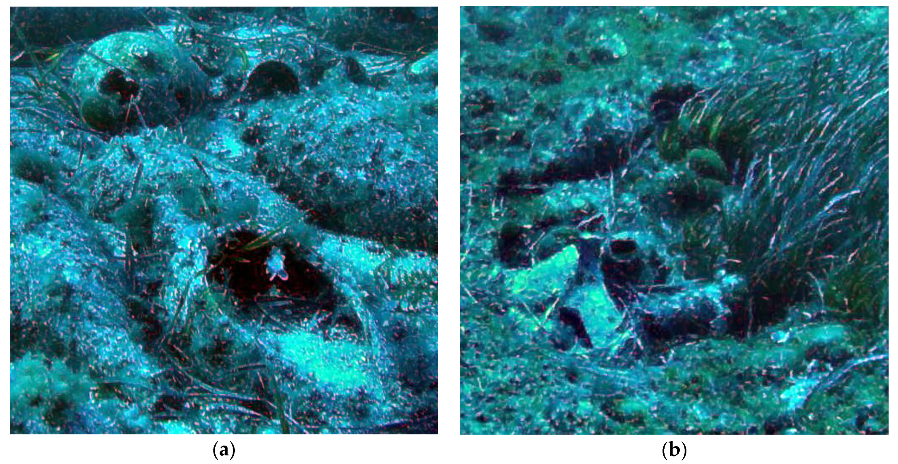
Along the same lines, we would like to report another particular case that is worth mentioning. Looking at Table 3 and Table 4, it is possible to conclude that the SP algorithm performed better than all the others according to all the three metrics in both cases of “CalaMinnola1” and “CalaMinnola2” (Figure 3).
In Figure 3 we can see a detail of “CalaMinnola1” and “CalaMinnola2” images enhanced with the SP algorithm. Looking at these images, it becomes quite clear that the SP algorithm in these cases have generated some ‘artefacts’, likely due to the oversaturation of some image details. This issue could probably be solved or attenuated by tuning the saturation parameter of the SP algorithm which we have fixed to a standard value, as we did for the parameters of the other algorithms, too. Anyway, the issue is that the metrics were misled by these ‘artefacts’, assigning a high value to the enhancement made by this algorithm.
Nonetheless, for each image in the dataset we have elaborated a table such as Table 2. Since it is neither practical nor useful to report all these tables here, we summarized them in a single one (Table 5).
Table 5 consists of five sections, one for each underwater site. Each of these sections reports the average values of the three metrics calculated for the related site. These average values are defined, within each site, as the arithmetic mean of the metrics calculated for the first, the second and the third sample image. Obviously, the calculation of these metrics was carried out for each algorithm on the three images enhanced using them. In fact, each column reports the metrics related to a given algorithm.
This table enables us to deduce more generalized considerations about the performances of the selected algorithms on our dataset of images. Focusing on the values in bold, we can deduce that the SP algorithm performed better at the sites of Baiae, Cala Cicala, Cala Minnola, and MazotosN, having the best total values in two out of three metrics (). Moreover, looking at the entropy (), i.e., the metric on which SP lost, we can recognize that the values calculated for this algorithm are not so far from the values calculated for the other algorithms. However, the ACE algorithm seems to be the one that performs best at enhancing the information entropy of the images. As regards the images taken on the underwater site of Mazotos with artificial light (MazotosA), the objective evaluation conducted with these metrics seems not to converge on any of the algorithms. Such an undefined result, along with the issues previously reported, are drawbacks caused by evaluating the underwater images relying only on quantitative metrics.
To sum up, even if the quantitative metrics can provide a useful indication about image quality, they do not seem reliable enough to be blindly employed for evaluating the performances of an underwater image enhancement algorithm. Hence, in the next section we shall describe an alternative methodology to evaluate the underwater image enhancement algorithms, based on a qualitative evaluation conducted with a panel of experts in the field of underwater imagery being members of iMARECULTURE project.
5. Benchmarking Based on Expert Panel
We designed an alternative methodology to evaluate the underwater image enhancement algorithms. A panel of experts in the field of underwater imagery (members of iMARECULTURE project) was assembled. This panel is composed of several professional figures from five different countries, such as underwater archaeologists, photogrammetry experts and computer graphics scientists with experience in underwater imagery. This panel expressed an evaluation on the quality of the enhancement conducted on the underwater images dataset through some selected algorithms.
5.1. Evaluation Methods
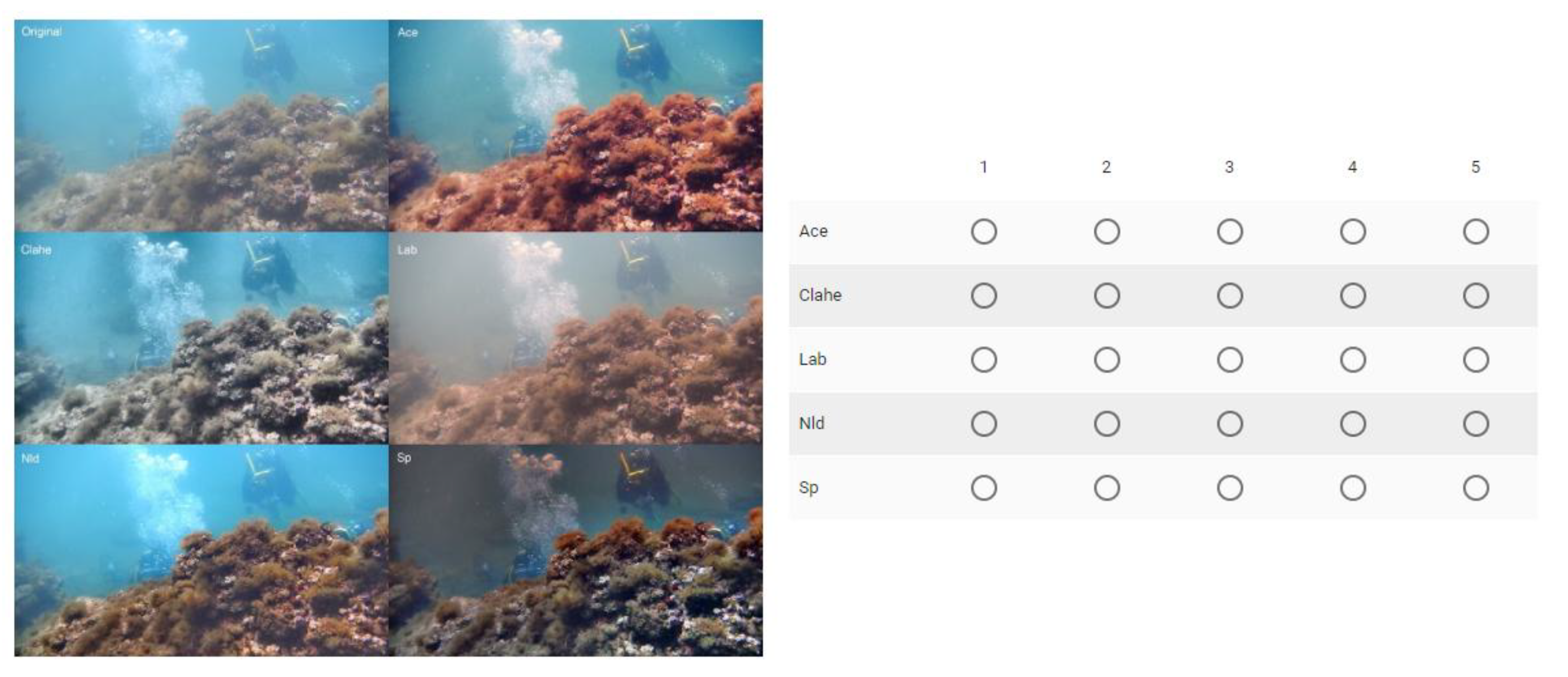
The dataset of images and the selected algorithms are the same ones that were employed and described in the previous section. A survey with all the original and enhanced images was created in order to be submitted to the expert panel. A questionnaire was set up for this purpose, a section of which is shown in Figure 4.
The questionnaire is composed of fifteen sections like the one shown in the picture; one for each of the fifteen images in the dataset. Each mosaic is composed of an original image and the same image enhanced with five different algorithms. Each of these underwater images are labelled with the acronym of the algorithm that produced them. Under the mosaic there is a multiple-choice table. Each row is labelled with the algorithm’s name and represents the image enhanced with the algorithm. For each of these images, the expert was to provide an evaluation expressed as a number from one to five, where “one” represents a very poor enhancement and “five” a very good one, considering both the effects of colour correction and contrast/sharpness enhancement. The hi-res images were provided separately to the experts in order to fulfil a better evaluation.
5.2. Results
All these evaluations, expressed by each expert on each enhanced image of our dataset, provide a lot of data that needs to be interpreted. A feasible way to aggregate all these data in order to extract some useful information is to calculate an average vote expressed by the experts on the images of a single site divided by algorithm. This average is calculated as a mean vote of the three images of the site.
The values in Table 6 show that ACE reached the higher average vote for the sites of Baiae, Cala Cicala and Cala Minnola and CLAHE has the higher average vote for Mazotos in both cases of artificial and natural light. It is worth noting that ACE gained a second place on Mazotos (both cases).
However, a simple comparison of these average values could be unsuitable from a statistical point of view. Consequently, we performed the ANOVA (ANalysis Of VAriance) on these data. The ANOVA is a statistical technique that compares different sources of variance within a dataset. The purpose of the comparison is to determine whether significant differences exist between two or more groups. In our specific case, the purpose is to determine whether the difference between the average vote of the algorithms is significant. Therefore, the groups for our ANOVA analysis are represented by each algorithm and the analysis is repeated for each site.
Table 7 shows the results of ANOVA test. A significance value below 0.05 entails that there is a significant difference between the means of our group.
The significance values for each site are reported in the last column and are all below the 0.05 threshold. This indicates that, for each site, there is a significant difference between the average value gained by each algorithm. However, this result is not enough, because it does not show which algorithms are effectively better than the others. Thus, we conducted a “post hoc” analysis, named Tukey’s HSD (Honest Significant Difference), which is a test that determines specifically which groups are significantly different. This test assumes that the variance within each group is similar; therefore, a test of homogeneity of variances is needed to establish whether this assumption can hold for our data.
Table 8 shows the results of the homogeneity test. The significance is reported in the last column and a value above 0.05 indicates that the variance between the algorithms is similar with regard to the related site. Cala Cicala and MazotosA have a significance value below 0.05, so for these two sites, the assumption of homogeneity of variances does not hold. We employed a different “post hoc” analysis for these two sites, i.e., Games-Howell, that does not require the assumption of equal variances.
The differences between the mean values, totalled for each algorithm at an underwater site, is significant at the level 0.05. Analysing the results reported in Table 6 and in Table 9, we produced this interpretation of the expert panel evaluation:
- Baiae: ACE and SP are better than LAB and NLD, whereas CLAHE does not show results significantly better or worse than the other algorithms.
- Cala Cicala: ACE is better than LAB and NLD. CLAHE is better than NLD.
- Cala Minnola: ACE is better than CLAHE, LAB and NLD. SP is significantly better than NLD but does not show significant differences with the other algorithms.
- MazotosA: ACE is better than NLD and SP. CLAHE is better than LAB, NLD and SP. There are no significant differences between ACE and CLAHE.
- MazotosN: CLAHE is better than LAB, NLD e SP. There are no significant differences between ACE and CLAHE.
In a nutshell, ACE works fine at all sites. CLAHE works as well as ACE at all sites except Cala Minnola. SP works fine too at the sites of Baiae, Cala Cicala and Cala Minnola.
Table 10 shows a simplified version of the analysis performed on the expert evaluation through ANOVA. The “Mean Vote” column reports the average vote expressed by all the experts on the three images related to the site and to the algorithm represented by the row. The rows are ordered by descending “Mean Vote” order within each site. The “Significance” column indicates if the related “Mean Vote” is significantly different from the higher “Mean Vote” at the related site. Consequently, the bold values indicate the algorithm with the higher “Mean Vote” for each site. The values highlighted in orange represent the algorithms with a “Mean Vote” not significantly different from the first one within the related site.
6. Benchmarking Based on the Results of 3D Reconstruction
Computer vision applications in underwater settings are particularly affected by the optical properties of the surrounding medium [50]. In the 3D underwater reconstruction process, the image enhancement is a necessary pre-processing step that is usually tackled with two different approaches. The first one focuses on the enhancement of the original underwater imagery before the 3D reconstruction in order to restore the underwater images and potentially improve the quality of the generated 3D point cloud. This approach in some cases of non-turbid water [34,35] proved to be unnecessary and time-consuming, while in high-turbidity water it seems to have been effective enough [46,51]. The second approach suggests that, in good visibility conditions, the colour correction of the produced textures or orthoimages is sufficient and time efficient [34,35]. This section presents the investigation as to whether and how the pre-processing of the underwater imagery using the five implemented image enhancement algorithms affects the 3D reconstruction using automated SfM-MVS software. Specifically, each one of the presented algorithms is evaluated according to its performance in improving the results of the 3D reconstruction using specific metrics over the reconstructed scenes of the five different datasets.
6.1. Evaluation Methods
To address the above research issues, five different datasets were selected to capture underwater imagery ensuring different environmental conditions (i.e., turbidity etc.), depth, and complexity. The five image enhancement methods already described were applied to these datasets. Subsequently, dense 3D point clouds (3Dpc) were generated for each dataset using a robust and reliable commercial SfM-MVS software. The produced 3D point clouds were then compared using Cloud Compare [52] open-source software and statistics were computed. The followed process is quite similar to the one presented in [34,35].
6.1.1. Test Datasets
The dataset used for the evaluations of the 3D reconstruction results was almost the same as the ones presented in Section 3.2. The only exception is that the MazotosN images used in this section were captured on an artificial reef constructed using 1-m-long amphorae, replicas from the Mazotos shipwreck [53]. Although the images of MazotosN were acquired in two different locations, all the images were captured by exactly the same camera under the same turbidity and illumination conditions. Moreover, both locations were at the same depth, thus resulting in the same loss of red colour in all of the images from both locations due to a strong absorption and scarce illumination typical of these depths. The images from the artificial reef present abrupt changes on the imaged object depth, thus causing a more challenging task for the 3D reconstruction
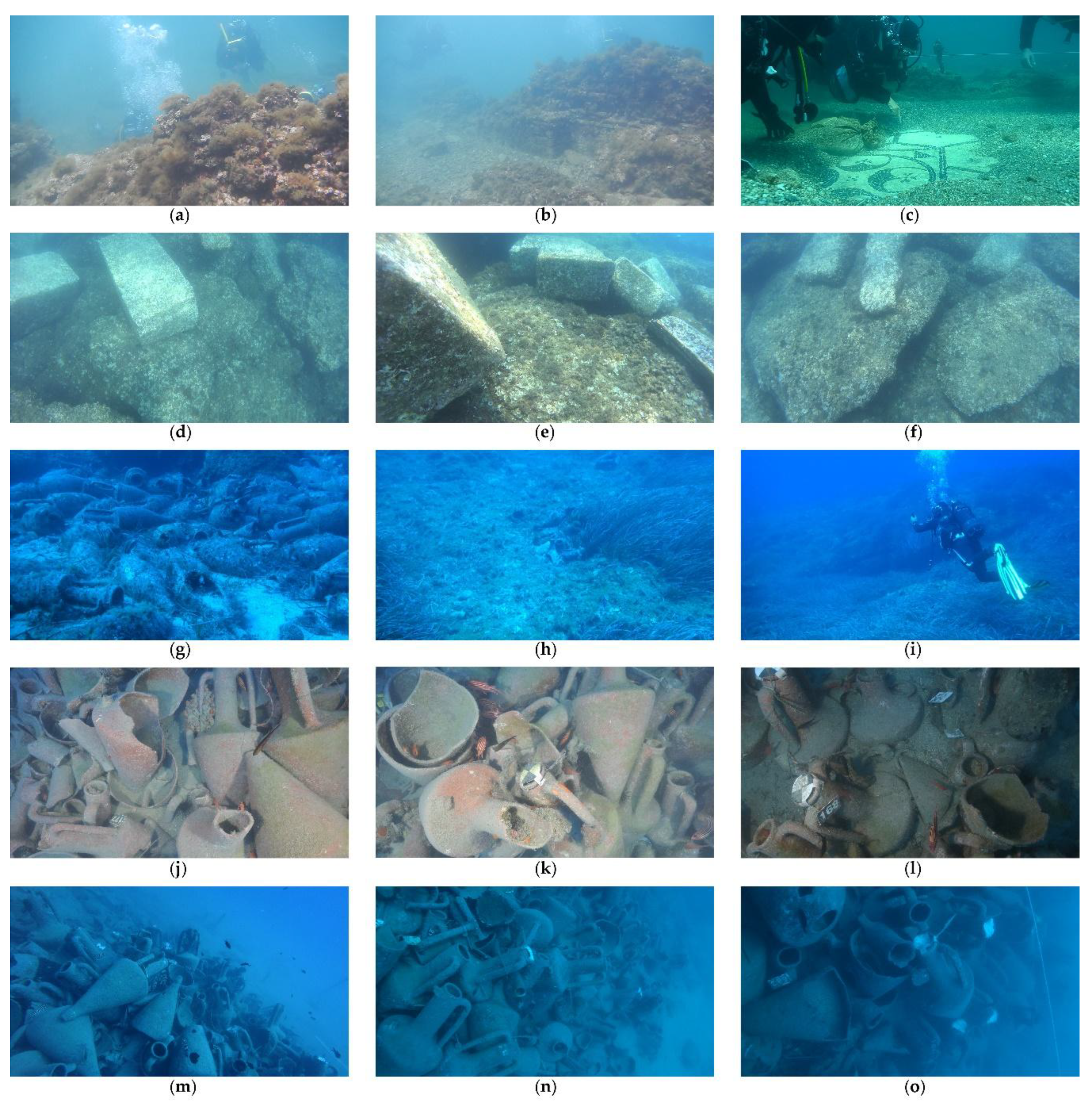
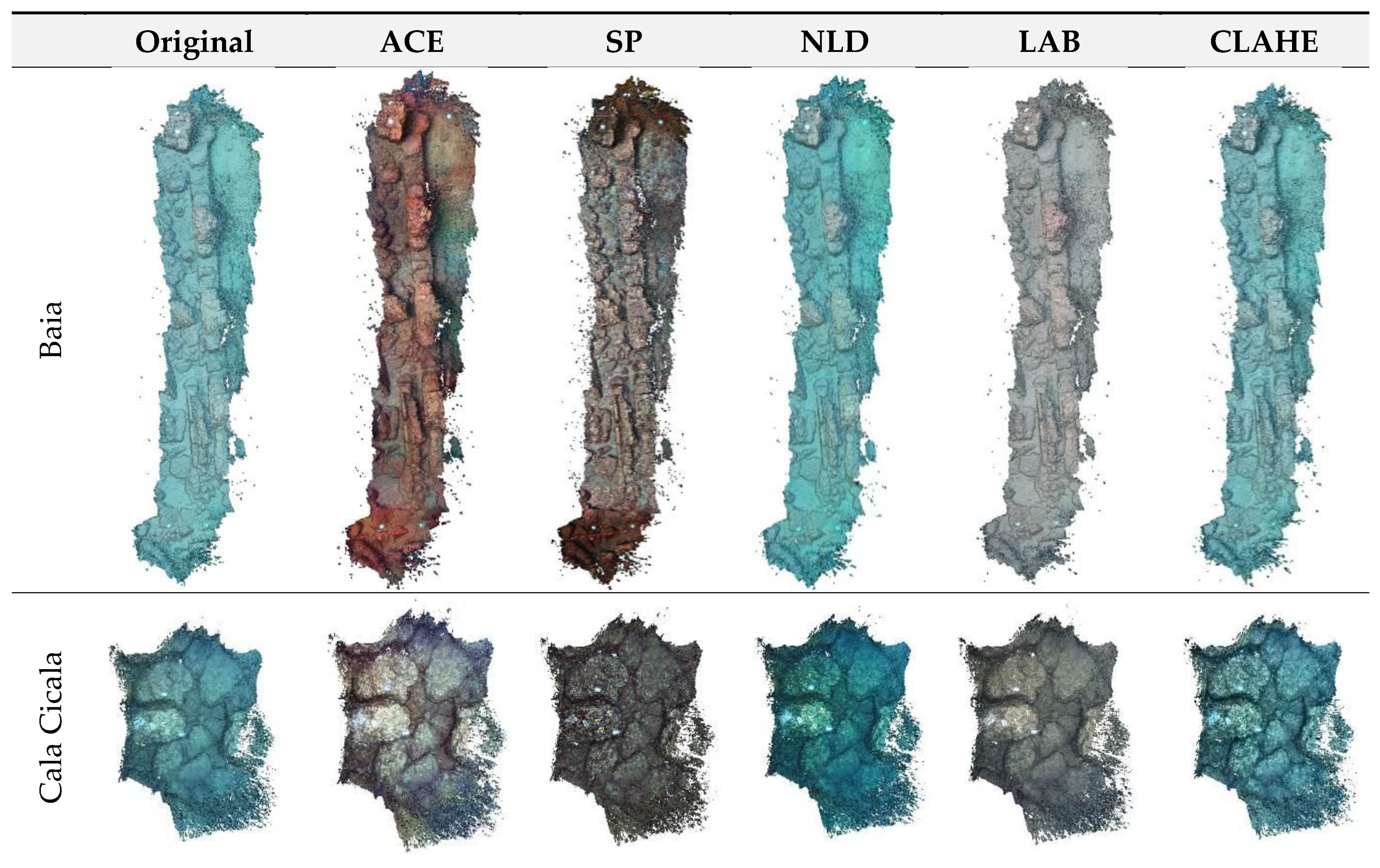
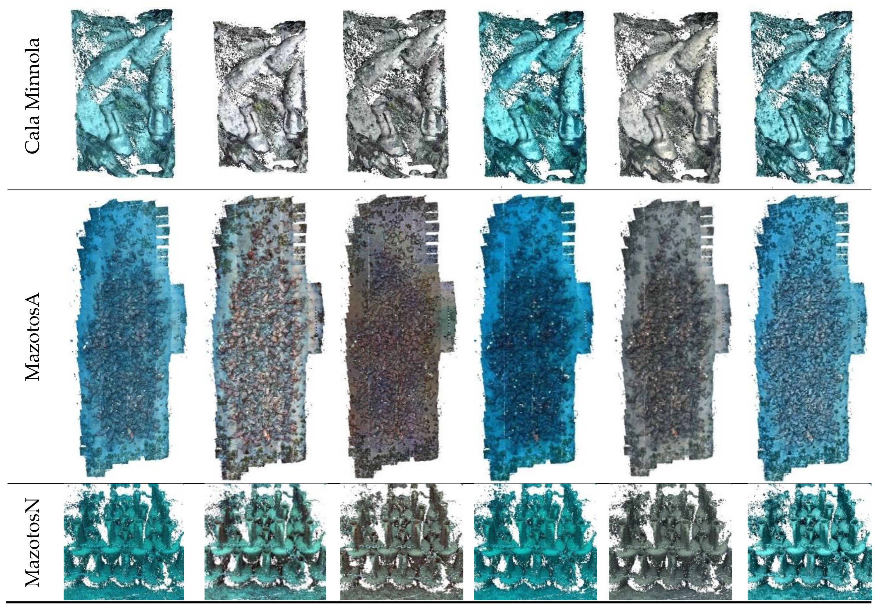
For evaluating the 3D reconstruction results, a large number of images of the datasets described above was used, having the required overlap as they were acquired for photogrammetric processing. Each row of Figure 5 represents a dataset, while in each column, the results of the five image enhancement algorithms, as well as the original image, are presented.
6.1.2. SfM-MVS Processing
Subsequently, enhanced imagery was processed using SfM-MVS with Agisoft’s Photoscan commercial software [38]. The main reason for using this specific software for the performed tests, instead of other commercial SfM-MVS software or SIFT [33] and SURF [39] detection and matching schemes, is that according to our experience in underwater archaeological 3D mapping projects, it proves to be one of the most robust and maybe the most commonly used among the underwater archaeological 3D mapping community [5]. For each site, six different 3Dpcs were created, one with each colour-corrected dataset (Figure 6): (i) One with the original uncorrected imagery, which is considered the initial solution, (ii) a second one using ACE, (iii) a third one using the imagery that resulted implementing SP the colour correction algorithm, (iv) a fourth one using NLD enhanced imagery, (v) a fifth one using LAB enhanced imagery, and (vi) a sixth one using CLAHE enhanced imagery. All three RGB channels of the images were used for these processes.
For the processing of each test site, the alignment and calibration parameters of the original (uncorrected) dataset were adopted. This ensured that the alignment parameters will not affect the dense image matching step and the comparisons between the generated point clouds can be realized. To scale the 3D dense point clouds, predefined Ground Control Points (GCPs) were used for calculating the alignment parameters of the original imagery to be also used for the enhanced imagery. The above procedure was adopted in order to ensure a common ground for the comparison of the 3D point clouds, since the data were of real-life applications and targeting control points for each dataset would introduce additional errors to the process (targeting errors, etc.). Subsequently, 3D dense point clouds of medium quality and density were created for each dataset. No filtering during this process was performed in order to obtain the total number of dense point clouds, as well as to evaluate the resulting noise. It should be noted that medium-quality dense point clouds mean that the initial images’ resolutions were reduced by a factor of 4 (2 times by each side) in order to be processed by the SfM-MVS software [38].
6.1.3. Metrics for Evaluating the Results of the 3D Reconstructions
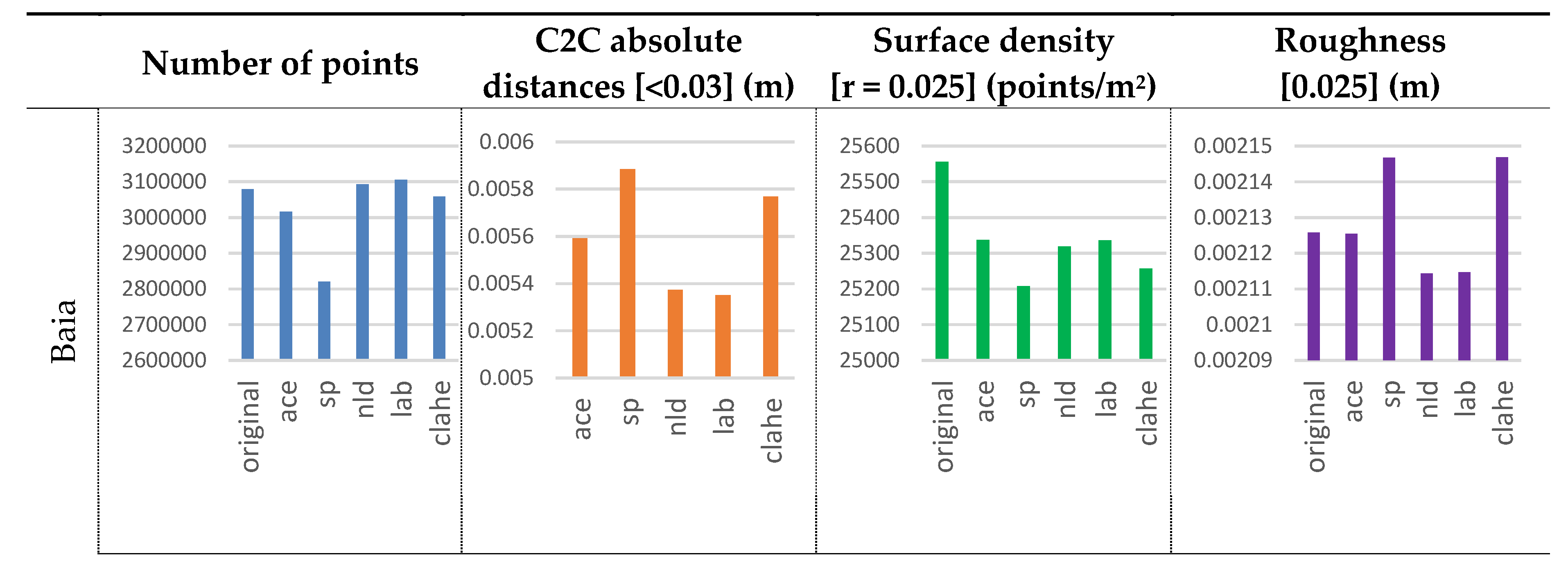
All the dense point clouds presented above (Figure 6) were imported into Cloud Compare freeware [52] for further investigation. In particular, the following parameters and statistics, used also in [54,55], were computed for each point cloud:
- Total number of points. All the 3D points of the point cloud were considered for this metric, including any outliers and noise [52]. For our purposes, the total number of 3D points reveal the effect of an algorithm on the matchable pixels between the images. The more corresponding pixels are found in the Dense Image Matching (DIM) step on the images, the more points are generated. Higher values of total number of points are considered better in these cases; however, this should be crosschecked with the point density metric, since it might be an indication of noise on the point cloud.
- Cloud to cloud distances. Cloud to cloud distances are computed by selecting two-point clouds. The default way to compute this kind of distance is the ‘nearest neighbour distance’: for each point of the compared cloud, Cloud Compare searches the nearest point in the reference cloud and computes the Euclidean distance between them [52]. This search was performed within a maximum distance of 0.03 m, since this is a reasonable accuracy for real-world underwater photogrammetric networks [56]. All points farther than this distance will not have their true distance computed—the threshold value will be used instead. For the performed tests, this metric is used to investigate the deviation of the “enhanced” point cloud, generated using the enhanced imagery, from the original one. However, since there are no reference point clouds for these real-world datasets, this metric is not used for the final evaluation. Nevertheless, this metric can be used as an indication of how much an algorithm affects the final 3D reconstruction. Small RMSE (Root Mean Square Error) means small changes; hence the algorithm is not that intrusive, nor effective.
- Surface Density. The density is estimated by counting the number of neighbours N (inside a sphere of radius R) for each point [52]. The surface density used for this evaluation is defined as , i.e., the number of neighbours divided by the neighbourhood surface. Cloud Compare estimates the surface density for all the points of the cloud and then it calculates the average value for an area of 1 m2 in a proportional way. Surface density is considered to be a positive metric, since it defines the number of the points on a potential generated surface, excluding the noise being present as points out of this surface. This is also the reason of using the surface density metric instead of the volume density metric.
- Roughness. For each point, the ‘roughness’ value is equal to the distance between this point and the best fitting plane computed on its nearest neighbours [52], which are the points within a sphere centred on the point. The radius of that sphere was set to 0.025 m for all datasets. This value was chosen as the maximum distance between two points in the less dense point cloud. Roughness is considered to be a negative metric since it is an indication of noise on the point cloud, assuming an overall smooth surface.
6.2. Results
The values of the computed metrics for the five different datasets and the five different image enhancement algorithms are presented in Figure 7. The following considerations can be deduced regarding each metric:
- Total number of points. SP algorithm produced the less 3D points in the 60% of the test cases while LAB produced more points than all the others, including the original datasets in the 80% of the test cases. In fact, only for the Cala Minnola dataset, the LAB points were noticeably less than the original points. Additionally, NLD images produced more points than the CLAHE-corrected imagery in 80% of the tests, and more points than the ACE-corrected imagery in 80% of the cases. ACE-corrected imagery always produced less points than the original imagery, except in the case of the Cala Minnola dataset.
- Cloud to cloud distances. The SP- and CLAHE-corrected imagery presented the greatest distances in 100% of the cases, while the NLD- and LAB-corrected imagery presented the smallest cloud to cloud distances in 100% of the cases. However, these deviations were less than 0.001 m in all the cases.
- Surface Density. In most of the cases, surface density was linear to the total number of points. However, this was not observed in the Baia dataset test, where LAB- and NLD-corrected imagery produced more points in the dense point cloud, although their surface density was less than the density of the point cloud of the original imagery. This is an indication of outlier points and noise in the dense point cloud. Volume density of the point clouds was also computed; however, it is not presented here, since it is linear to the surface density.
- Roughness. SP-corrected imagery produced the roughest point cloud in the 60% of the cases, while for MazotosA dataset the roughest was the original point cloud. LAB and NLD corrected imagery seemed to produce almost equal or less noise than the original imagery in most of the cases.
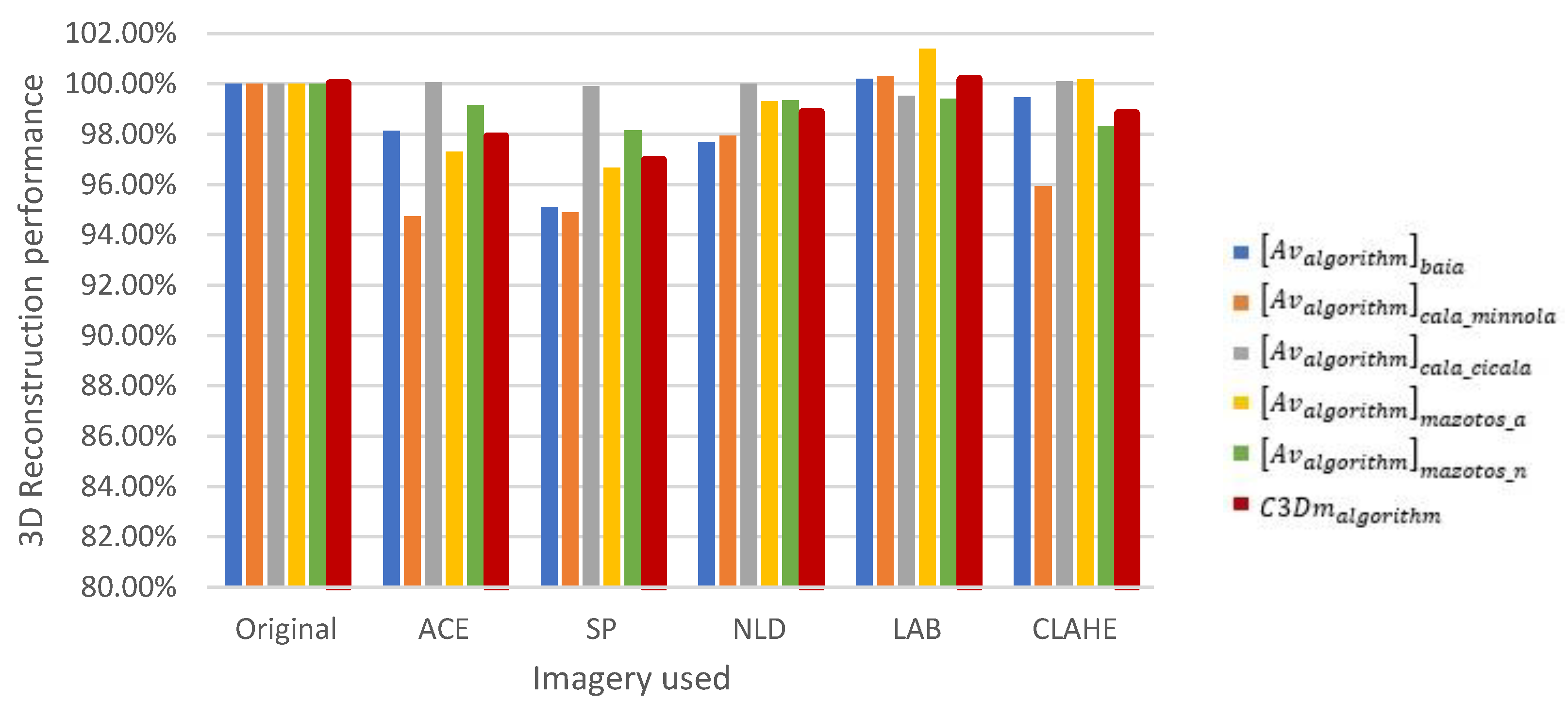
To facilitate an overall comparison of the tested algorithms in terms of 3D reconstruction performance and evaluate the numerous results presented above, the surface density D and roughness R metrics were normalized and combined into one overall metric, named as the Combined 3D metric (C3Dm). To achieve that, the score of every image enhancement algorithm on D and R was normalized to the score of the 3D reconstruction computed using the original images. Hence, the 100% score is referred to the original 3D reconstruction. If an image enhancement algorithm has a negative impact on the 3D reconstruction, then the score should be less than 100% and if it has a positive impact, the score should be more than 100%. For both surface density D and roughness R, the same weight was used.
The score totalled for each algorithm was computed independently for each dataset as the average value () of the normalized metrics (Equation (2)). The same computation was performed to calculate the score () of each original reconstruction for each original dataset (Equation (1)). The C3Dm was computed for each algorithm summing up the scores totalized by the algorithm on each dataset and normalizing it to the score totalized by the original images (Equation (3)).
The total number of points and the Cloud to cloud distances metrics were not used for the computation of the C3Dm. The reason for this is that the first one is highly correlated with the surface density metric, while the second one is not based on reference data that could have been used as ground truth. However, these two metrics were used individually to deduce some valuable considerations in the performance of the tested algorithms.
Figure 8 shows the for each algorithm and each dataset, and the for each dataset. The results, that are also presented in Table 11, suggest that the LAB algorithm improves the 3D reconstruction in most of the cases, while the other tested algorithms do not, and they do have a negative effect on it. However, the final is not significantly different from the one of the other algorithms. Consequently, LAB performs better than the others, while CLAHE follows up with almost 1.4% difference.
ACE and SP seem to produce the least valuable results, in terms of 3D reconstruction, and this was expected, since the enhanced imagery resulted by these algorithms in some cases has generated some ‘artefacts,’ likely due to the oversaturation of some image details. However, the differences on the performance are less than 4%.
In conclusion, the most remarkable consideration that arises from Table 11 is that four out of five algorithms worsen the results of the 3D reconstruction process and only the LAB slightly improves the results.
7. Comparison of the Three Benchmarks Results
According to the objective metrics results reported in Section 4, the SP algorithm seemed to perform better than the others in all the underwater sites, except for the case MazotosA. For these images, taken on Mazotos with artificial light, each metric assigned a higher value to a different algorithm, preventing us from deciding which algorithm performed better on this dataset. It is also worth to remember that the ACE algorithm seems to be the one that performs better in enhancing the information entropy of the images. However, objective metrics do not seem consistent nor significantly different enough to allow the best algorithm nomination. On the other hand, the opinion of experts seems to be that the ACE algorithm is the one that performs better on all sites, and CLAHE and SP perform as fine as ACE at some sites. Additionally, the 3D reconstruction quality seems to be decreased by all the algorithms, except LAB that slightly improves it.
Table 12 shows a comparison between average objective metrics, average vote of experts and C3Dm divided by site. The best score for each evaluation is marked in bold. Let us recall that the values highlighted in orange in the expert evaluation rows (Exp) are not significantly different from each other within the related site. It is worth noting that the objective metric that seems to get closest to the expert opinion is , i.e., information entropy. Indeed, is consistent with the expert opinion, regarding the nomination of the best algorithm within the related site, in all the five sites. and are consistent with each other on 4/5 sites and with the expert opinion on 3/5 sites.
To recap, the concise result of the objective and expert evaluation seems to be that LAB and NLD do not perform as well as the other algorithms. ACE could be employed in different environmental condition with good results. CLAHE and SP can produce a good enhancement in some environmental conditions.
On the other hand, according to the evaluation based on the results of 3D reconstruction, the LAB algorithm seems to have the best performance, producing more 3D points, insignificant cloud to cloud distances, high surface density and low roughness 3D point clouds.
8. Conclusions
We have selected five well-known state-of-the-art methods of the enhancement of images taken on various underwater sites with five different environmental and illumination conditions. We have produced a benchmark for these methods based on three different evaluation techniques:
- an objective evaluation based on metrics selected among those already adopted in the field of underwater image enhancement;
- a subjective evaluation based on a survey conducted with a panel of experts in the field of underwater imagery;
- an evaluation based on the improvement that these methods may bring to 3D reconstructions.
Our purpose was twofold. First of all, we tried to establish which methods perform better than the others and whether or not there existed an image enhancement method, among the selected ones, that could be employed seamlessly in different environmental conditions in order to accomplish different tasks such as visual enhancement, colour correction and 3D reconstruction improvement.
The second aspect was the comparison of the three above mentioned evaluation techniques in order to understand if they provide consistent results. Starting from the second aspect, we can state that the 3D reconstructions are not significantly improved by discussed methods, probably the minor improvement obtainable with the LAB could not justify the effort to pre-process hundreds or thousands of images required for larger models. On the other hand, the subjective metrics and the expert panel appear to be quietly consistent and, in particular, the identifies the same best methods of the expert panel on all the dataset. Consequently, an important conclusion that can be drawn from this analysis is that should be adopted in order to have an objective evaluation that provides results consistent with the judgement of qualitative evaluations performed by experts in image enhancement. This is an interesting point, because it is not so easy to organize an expert panel for such kind of benchmark.
On the basis of these considerations, we can compare the five selected methods by means of the objective metrics (in particular ) and the expert panel. It is quite apparent from Table 12 that ACE, in almost all the environmental conditions, is the one that improves the underwater images more than the others. In some cases, SP and CLAHE can lead to similar good results.
Moreover, thanks to the tool described in Section 2 and provided in Supplementary Materials, the community working in underwater imaging would be able to quickly generate a dataset of enhanced images processed with five state of the art methods and use them in their works or to compare new methods. For instance, in case of an underwater 3D reconstruction, our tool can be employed to try different combinations of methods and quickly verify if the reconstruction process can be improved somehow. A possible strategy could be to pre-process the images with the LAB method trying to produce a more accurate 3D model and, afterwards, to enhance the original images with another method such as ACE to achieve a textured model more faithful to the reality (Figure 9). Employing our tool for the enhancement of the underwater images ensures to minimize the pre-processing effort and enables the underwater community to quickly verify the performance of the different methods on their own datasets.
Finally, Table 13 summarizes our conclusions and provides the community with some more categorical guidelines regarding which method should be used according to different underwater conditions and tasks. In this table, the visual enhancement row refers to the improvement of the sharpness, contrast and colour of the images. The 3D Reconstruction row refers to the improvement of the 3D model, apart from the texture. As previously described, the texture of the model should be enhanced with a different method, according to the environmental conditions and, therefore, to the previous “visual enhancement” guidelines. Furthermore, as far as the evaluation of other methods that have not debated here is concerned, our guideline is to evaluate them with the metric, as pursuant to our results, it is the metric that is closest to the expert panel evaluation.
In the end, let us underline, though, that we are fully aware of the fact that there are several other methods for underwater image enhancement and manifold metrics for the evaluation of these methods. It was not possible to debate them all in a single paper. Our effort has been to guide the community towards the definition of a more effective and objective methodology for the evaluation of the underwater image enhancement methods.
Supplementary Materials
The “Software Tool for Enhancing Underwater Images” is available online at http://www.imareculture.eu/project-tools.html.
Author Contributions
Funding
The work presented here is in the context of iMareCulture project (Advanced VR, iMmersive Serious Games and Augmented REality as Tools to Raise Awareness and Access to European Underwater CULTURal heritagE, Digital Heritage) that has received funding from the European Union’s Horizon 2020 research and innovation programme under grant agreement No. 727153.
Acknowledgments
The authors would like to thank the Department of Fisheries and Marine Research of Cyprus for the creation and permission to use the artificial amphorae reef (MazotosN).
Conflicts of Interest
The authors declare no conflict of interest.
References
- MareCulture. Available online: http://www.imareculture.eu/ (accessed on 8 January 2018).
- Bruno, F.; Lagudi, A.; Ritacco, G.; Čejka, J.; Kouřil, P.; Liarokapis, F.; Agrafiotis, P.; Skarlatos, D.; Philpin-Briscoe, O.; Poullis, C. Development and integration of digital technologies addressed to raise awareness and access to European underwater cultural heritage: An overview of the H2020 i-MARECULTURE project. In Proceedings of the OCEANS 2017, Aberdeen, UK, 19–22 June 2017. [Google Scholar]
- Skarlatos, D.; Agrafiotis, P.; Balogh, T.; Bruno, F.; Castro, F.; Petriaggi, B.D.; Demesticha, S.; Doulamis, A.; Drap, P.; Georgopoulos, A.; et al. Project iMARECULTURE: Advanced VR, iMmersive Serious Games and Augmented REality as Tools to Raise Awareness and Access to European Underwater CULTURal heritagE. In Digital Heritage: Progress in Cultural Heritage: Documentation, Preservation, and Protection; Ioannides, M., Fink, E., Moropoulou, A., Hagedorn-Saupe, M., Fresa, A., Liestøl, G., Rajcic, V., Grussenmeyer, P., Eds.; Lecture Notes in Computer Science; Springer: New York, NY, USA, 2016; pp. 805–813. [Google Scholar]
- Mangeruga, M.; Cozza, M.; Bruno, F. Evaluation of Underwater Image Enhancement Algorithms under Different Environmental Conditions. J. Mar. Sci. Eng. 2018, 6, 10. [Google Scholar] [CrossRef]
- Menna, F.; Agrafiotis, P.; Georgopoulos, A. State of the art and applications in archaeological underwater 3D recording and mapping. J. Cult. Herit. 2018, 33, 231–248. [Google Scholar] [CrossRef]
- Han, M.; Lyu, Z.; Qiu, T.; Xu, M. A Review on Intelligence Dehazing and Color Restoration for Underwater Images. IEEE Trans. Syst. Man Cybern. Syst. 2018. [Google Scholar] [CrossRef]
- He, K.; Sun, J.; Tang, X. Single Image Haze Removal Using Dark Channel Prior. IEEE Trans. Pattern Anal. Mach. Intell. 2011, 33, 2341–2353. [Google Scholar] [CrossRef] [PubMed] [Green Version]
- Drews, P.; Nascimento, E.; Moraes, F.; Botelho, S.; Campos, M. Transmission Estimation in Underwater Single Images. In Proceedings of the IEEE International Conference on Computer Vision Workshops, Sydney, Australia, 1–8 December 2013; pp. 825–830. [Google Scholar]
- Fattal, R. Single image dehazing. ACM Trans. Graph. (TOG) 2008, 27, 72. [Google Scholar] [CrossRef]
- Fattal, R. Dehazing using color-lines. ACM Trans. Graph. (TOG) 2014, 34, 13. [Google Scholar] [CrossRef]
- Berman, D.; Avidan, S. Non-local image dehazing. In Proceedings of the IEEE Conference on Computer Vision and Pattern Recognition, Las Vegas, NV, USA, 26 June–1 July 2016; pp. 1674–1682. [Google Scholar]
- Berman, D.; Treibitz, T.; Avidan, S. Air-light estimation using haze-lines. In Proceedings of the 2017 IEEE International Conference on Computational Photography (ICCP), Stanford, CA, USA, 12–14 May 2017; pp. 1–9. [Google Scholar]
- Sankpal, S.S.; Deshpande, S.S. Nonuniform Illumination Correction Algorithm for Underwater Images Using Maximum Likelihood Estimation Method. J. Eng. 2016, 2016. [Google Scholar] [CrossRef]
- Morel, J.-M.; Petro, A.-B.; Sbert, C. Screened Poisson Equation for Image Contrast Enhancement. Image Process. On Line 2014, 4, 16–29. [Google Scholar] [CrossRef] [Green Version]
- Carlevaris-Bianco, N.; Mohan, A.; Eustice, R.M. Initial results in underwater single image dehazing. In Proceedings of the OCEANS 2010, Seattle, WA, USA, 20–23 September 2010; pp. 1–8. [Google Scholar]
- Bianco, G.; Muzzupappa, M.; Bruno, F.; Garcia, R.; Neumann, L. A new color correction method for underwater imaging. Int. Arch. Photogramm. Remote Sens. Spat. Inf. Sci. 2015, 40, 25. [Google Scholar] [CrossRef]
- Bianco, G.; Neumann, L. A fast enhancing method for non-uniformly illuminated underwater images. In Proceedings of the OCEANS 2017, Anchorage, AL, USA, 18–22 September 2017; pp. 1–6. [Google Scholar]
- Gatta, C.; Rizzi, A.; Marini, D. Ace: An automatic color equalization algorithm. In Proceedings of the Conference on Colour in Graphics, Imaging, and Vision, Poitiers, France, 2–5 April 2002; Volume 2002, pp. 316–320. [Google Scholar]
- Getreuer, P. Automatic Color Enhancement (ACE) and its Fast Implementation. Image Process. On Line 2012, 2, 266–277. [Google Scholar] [CrossRef] [Green Version]
- Pizer, S.M.; Amburn, E.P.; Austin, J.D.; Cromartie, R.; Geselowitz, A.; Greer, T.; ter Haar Romeny, B.; Zimmerman, J.B.; Zuiderveld, K. Adaptive histogram equalization and its variations. Comput. Vis. Graph. Image Process. 1987, 39, 355–368. [Google Scholar] [CrossRef]
- Zuiderveld, K. Contrast limited adaptive histogram equalization. In Graphics Gems IV; Academic Press Professional, Inc.: Cambridge, MA, USA, 1994; pp. 474–485. [Google Scholar]
- Singh, R.; Biswas, M. Contrast and color improvement based haze removal of underwater images using fusion technique. In Proceedings of the 2017 4th International Conference on Signal Processing, Computing and Control (ISPCC), Solan, India, 21–23 September 2017; pp. 138–143. [Google Scholar]
- Ancuti, C.O.; Ancuti, C.; Vleeschouwer, C.D.; Neumann, L.; Garcia, R. Color transfer for underwater dehazing and depth estimation. In Proceedings of the 2017 IEEE International Conference on Image Processing (ICIP), Beijing, China, 17–20 September 2017; pp. 695–699. [Google Scholar]
- Galdran, A.; Pardo, D.; Picón, A.; Alvarez-Gila, A. Automatic Red-Channel underwater image restoration. J. Vis. Commun. Image Represent. 2015, 26, 132–145. [Google Scholar] [CrossRef] [Green Version]
- Łuczyński, T.; Birk, A. Underwater Image Haze Removal and Color Correction with an Underwater-ready Dark Channel Prior. arXiv 2018, arXiv:1807.04169. [Google Scholar]
- Lu, J.; Li, N.; Zhang, S.; Yu, Z.; Zheng, H.; Zheng, B. Multi-scale adversarial network for underwater image restoration. Opt. Laser Technol. 2018. [Google Scholar] [CrossRef]
- Li, C.Y.; Cavallaro, A. Background Light Estimation for Depth-Dependent Underwater Image Restoration. In Proceedings of the 2018 25th IEEE International Conference on Image Processing (ICIP), Athens, Greece, 7–10 October 2018; pp. 1528–1532. [Google Scholar]
- Anwar, S.; Li, C.; Porikli, F. Deep Underwater Image Enhancement. arXiv 2018, arXiv:1807.03528. [Google Scholar]
- Nomura, K.; Sugimura, D.; Hamamoto, T. Underwater Image Color Correction using Exposure-Bracketing Imaging. IEEE Signal Process. Lett. 2018, 25, 893–897. [Google Scholar] [CrossRef]
- Chang, H.; Cheng, C.; Sung, C. Single Underwater Image Restoration Based on Depth Estimation and Transmission Compensation. IEEE J. Ocean. Eng. 2018. [Google Scholar] [CrossRef]
- Ancuti, C.; Ancuti, C.O.; Haber, T.; Bekaert, P. Enhancing underwater images and videos by fusion. In Proceedings of the 2012 IEEE Conference on Computer Vision and Pattern Recognition, Providence, RI, USA, 16–21 June 2012; pp. 81–88. [Google Scholar]
- Ancuti, C.O.; Ancuti, C.; Vleeschouwer, C.D.; Bekaert, P. Color Balance and Fusion for Underwater Image Enhancement. IEEE Trans. Image Process. 2018, 27, 379–393. [Google Scholar] [CrossRef] [PubMed]
- Lowe, D.G. Object recognition from local scale-invariant features. In Proceedings of the Seventh IEEE International Conference on Computer Vision, Kerkyra, Greece, 20–27 September 1999; Volume 2, pp. 1150–1157. [Google Scholar]
- Agrafiotis, P.; Drakonakis, G.I.; Georgopoulos, A.; Skarlatos, D. The Effect of Underwater Imagery Radiometry on 3d Reconstruction and Orthoimagery. ISPRS-Int. Arch. Photogramm. Remote Sens. Spat. Inf. Sci. 2017. [Google Scholar] [CrossRef]
- Agrafiotis, P.; Drakonakis, G.I.; Skarlatos, D.; Georgopoulos, A. Underwater Image Enhancement before Three-Dimensional (3D) Reconstruction and Orthoimage Production Steps: Is It Worth? In Latest Developments in Reality-Based 3D Surveying and Modelling; Remondino, F., Georgopoulos, A., González-Aguilera, D., Agrafiotis, P., Eds.; MDPI: Basel, Switzerland, 2018; ISBN 978-3-03842-685-1. [Google Scholar]
- Agrafiotis, P.; Skarlatos, D.; Forbes, T.; Poullis, C.; Skamantzari, M.; Georgopoulos, A. Underwater photogrammetry in very shallow waters: Main challenges and caustics effect removal. Int. Arch. Photogramm. Remote Sens. Spat. Inf. Sci. 2018, 42. [Google Scholar] [CrossRef]
- Forbes, T.; Goldsmith, M.; Mudur, S.; Poullis, C. DeepCaustics: Classification and Removal of Caustics From Underwater Imagery. IEEE J. Ocean. Eng. 2018. [Google Scholar] [CrossRef]
- Agisoft, L.L.C. Agisoft PhotoScan User Manual: Professional Edition; Agisoft LLC: St. Petersburg, Russia, 2017. [Google Scholar]
- Bay, H.; Tuytelaars, T.; Van Gool, L. SURF: Speeded Up Robust Features. In European Conference on Computer Vision, Proceedings of the 9th European Conference on Computer Vision, Graz, Austria, 7–13 May 2006; Leonardis, A., Bischof, H., Pinz, A., Eds.; Lecture Notes in Computer Science; Springer: Berlin/Heidelberg, Germany, 2006; pp. 404–417. [Google Scholar]
- Fischler, M.A.; Bolles, R.C. Random Sample Consensus: A Paradigm for Model Fitting with Applications to Image Analysis and Automated Cartography. Commun. ACM 1981, 24, 381–395. [Google Scholar] [CrossRef]
- OpenCV Library. Available online: https://opencv.org/ (accessed on 4 December 2017).
- Eigen. Available online: http://eigen.tuxfamily.org/index.php (accessed on 4 December 2017).
- FLANN-Fast Library for Approximate Nearest Neighbors: FLANN-FLANN Browse. Available online: https://www.cs.ubc.ca/research/flann/ (accessed on 4 December 2017).
- Limare, N.; Lisani, J.-L.; Morel, J.-M.; Petro, A.B.; Sbert, C. Simplest Color Balance. Image Process. On Line 2011, 1, 297–315. [Google Scholar] [CrossRef]
- FFTW Home Page. Available online: http://www.fftw.org/ (accessed on 4 December 2017).
- Bruno, F.; Lagudi, A.; Gallo, A.; Muzzupappa, M.; Davidde Petriaggi, B.; Passaro, S. 3D Documentation of Archeological Remains in the Underwater Park of Baiae. Int. Arch. Photogramm. Remote Sens. Spat. Inf. Sci. 2015. [Google Scholar] [CrossRef]
- Bruno, F.; Barbieri, L.; Lagudi, A.; Medaglia, S.; Miriello, D.; Muzzupappa, M.; Taliano Grasso, A. Survey and documentation of the “Cala Cicala” shipwreck. In Proceedings of the IMEKO International Conference on Metrology for Archaeology and Cultural Heritage, Lecce, Italy, 23–25 October 2017. [Google Scholar]
- Qing, C.; Yu, F.; Xu, X.; Huang, W.; Jin, J. Underwater video dehazing based on spatial–temporal information fusion. Multidimens. Syst. Signal Process. 2016, 27, 909–924. [Google Scholar] [CrossRef]
- Xie, Z.-X.; Wang, Z.-F. Color image quality assessment based on image quality parameters perceived by human vision system. In Proceedings of the 2010 IEEE International Conference on Multimedia Technology (ICMT), Ningbo, China, 29–31 October 2010; pp. 1–4. [Google Scholar]
- von Lukas, U.F. Underwater visual computing: The grand challenge just around the corner. IEEE Comput. Graph. Appl. 2016, 36, 10–15. [Google Scholar] [CrossRef] [PubMed]
- Mahiddine, A.; Seinturier, J.; Boï, D.P.J.; Drap, P.; Merad, D.; Long, L. Underwater image preprocessing for automated photogrammetry in high turbidity water: An application on the Arles-Rhone XIII roman wreck in the Rhodano river, France. In Proceedings of the 2012 18th International Conference on Virtual Systems and Multimedia, Milan, Italy, 2–5 September 2012; pp. 189–194. [Google Scholar]
- CloudCompare (Version 2.10 alpha) [GPL Software]. 2016. Available online: http://www.cloudcompare.org/ (accessed on 20 July 2018).
- Demesticha, S. The 4th-Century-BC Mazotos Shipwreck, Cyprus: A preliminary report. Int. J. Naut. Archaeol. 2011, 40, 39–59. [Google Scholar] [CrossRef]
- Remondino, F.; Nocerino, E.; Toschi, I.; Menna, F. A Critical Review of Automated Photogrammetric Processing of Large Datasets. Int. Arch. Photogramm. Remote Sens. Spat. Inf. Sci. 2017, 42. [Google Scholar] [CrossRef]
- Tefera, Y.; Poiesi, F.; Morabito, D.; Remondino, F.; Nocerino, E.; Chippendale, P. 3DNOW: Image-based 3D reconstruction and modeling via WEB. Int. Arch. Photogramm. Remote Sens. Spat. Inf. Sci. ISPRS Arch. 2018, 42, 1097–1103. [Google Scholar] [CrossRef]
- Skarlatos, D.; Agrafiotis, P.; Menna, F.; Nocerino, E.; Remondino, F. Ground control networks for underwater photogrammetry in archaeological excavations. In Proceedings of the 3rd IMEKO International Conference on Metrology for Archaeology and Cultural Heritage, Lecce, Italy, 23–25 October 2017; pp. 23–25. [Google Scholar]
Figure 1.
Underwater images dataset. (a–c) Images acquired at Underwater Archaeological Park of Baiae, named respectively Baia1, Baia2, Baia3. Credits: MiBACT-ISCR; (d–f) Images acquired at Cala Cicala shipwreck, named respectively CalaCicala1, CalaCicala2, CalaCicala3. Credits: Soprintendenza Belle Arti e Paesaggio per le province di CS, CZ, KR and University of Calabria; (g–i) Images acquired at Cala Minnola, named CalaMinnola1, CalaMinnola2, CalaMinnola3, respectively. Credits: Soprintendenza del Mare and University of Calabria; (j–l) Images acquired at Mazotos with artificial light, named respectively MazotosA1, MazotosA2, MazotosA3. Credits: MARELab, University of Cyprus; (m–o) Images acquired at Mazotos with natural light, named respectively MazotosN4, MazotosN5, MazotosN6. Credits: MARELab, University of Cyprus.

Figure 2.
The image “MazotosN4” enhanced with all five algorithms. (a) Original image; (b) Enhanced with ACE; (c) Enhanced with CLAHE; (d) Enhanced with LAB; (e) Enhanced with NLD; (f) Enhanced with SP.
Figure 2.
The image “MazotosN4” enhanced with all five algorithms. (a) Original image; (b) Enhanced with ACE; (c) Enhanced with CLAHE; (d) Enhanced with LAB; (e) Enhanced with NLD; (f) Enhanced with SP.


Figure 3.
Artefacts in the sample images “CalaMinnola1” (a) and “CalaMinnola2” (b) enhanced with SP algorithm.
Figure 3.
Artefacts in the sample images “CalaMinnola1” (a) and “CalaMinnola2” (b) enhanced with SP algorithm.

Figure 4.
A sample section of the survey submitted to the expert panel.

Figure 5.
Examples of original and corrected images of the 5 different datasets. Credits: MiBACT-ISCR (Baiae images); Soprintendenza Belle Arti e Paesaggio per le province di CS, CZ, KR and University of Calabria (Cala Cicala images); Soprintendenza del Mare and University of Calabria (Cala Minnola images); MARELab, University of Cyprus (MazotosA images); Department of Fisheries and Marine Research of Cyprus (MazotosN images).

Figure 6.
The dense point clouds for all the datasets and for all the available imagery.


Figure 7.
The results of the computed parameters for the five different datasets.


Figure 8.
The Combined 3D metric (C3Dm), representing an overall evaluation of 3D reconstruction performance of the five tested image enhancing methods on the five datasets.
Figure 8.
The Combined 3D metric (C3Dm), representing an overall evaluation of 3D reconstruction performance of the five tested image enhancing methods on the five datasets.

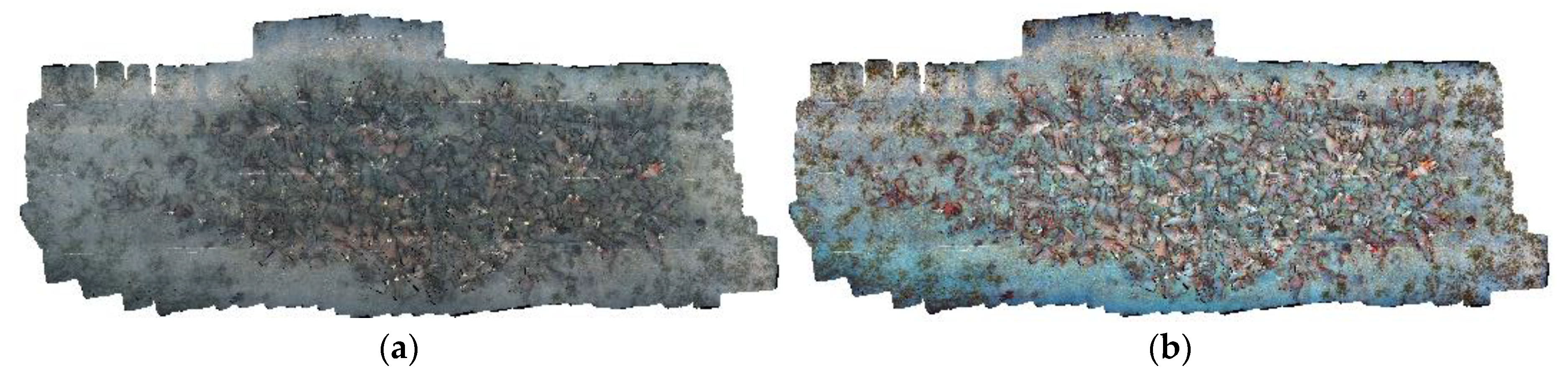
Figure 9.
Textured 3D models based on MazotosA dataset and created with two different strategies. (a) 3D model created by means of only LAB enhanced imagery both for the 3D reconstruction and texture. (b) 3D model created following the methodology suggested above: the 3D reconstruction was performed using the LAB enhanced imagery and the texturing using the more faithful to the reality ACE imagery.


Table 1.
Running times (seconds) of different algorithms on a sample image of 4000 × 3000 pixels.
| ACE | SP | NLD | LAB | CLAHE |
|---|---|---|---|---|
| 30.6 | 21.2 | 283 | 9.8 | 1.7 |
Table 2.
Results of benchmarking performed on “MazotosN4” image with the objective metrics.
| Metric | Original | ACE | SP | NLD | LAB | CLAHE | |
|---|---|---|---|---|---|---|---|
| 1 | 13.6907 | 61.6437 | 102.6797 | 10.9816 | 83.6466 | 39.8337 | |
| 105.3915 | 119.5308 | 118.5068 | 110.1816 | 98.1805 | 119.2274 | ||
| 170.9673 | 126.7339 | 115.2361 | 181.4046 | 109.9632 | 185.5852 | ||
| 96.6832 | 102.6361 | 112.1409 | 100.8559 | 97.2635 | 114.8821 | ||
| 2 | 4.6703 | 6.3567 | 6.7489 | 3.7595 | 6.6936 | 6.4829 | |
| 6.6719 | 7.4500 | 7.1769 | 6.6726 | 6.8375 | 7.2753 | ||
| 7.1811 | 7.5279 | 7.1045 | 7.2187 | 6.9055 | 7.3364 | ||
| 6.2688 | 7.1316 | 7.0126 | 6.0764 | 6.8128 | 7.0423 | ||
| 3 | 0.9600 | 2.6480 | 6.1200 | 1.0462 | 1.0752 | 2.4432 | |
| 1.0069 | 2.4210 | 3.9631 | 1.0958 | 1.0870 | 2.4754 | ||
| 1.1018 | 2.4332 | 4.2334 | 1.1566 | 1.1235 | 2.4776 | ||
| 1.0229 | 2.5007 | 4.7722 | 1.0995 | 1.0952 | 2.4654 | ||
1 Mean brightness (less is better). 2 Information entropy (more is better). 3 Average gradient (more is better).
Table 3.
Average metrics for the sample image “CalaMinnola1” enhanced with all algorithms.
| Metric | Original | ACE | SP | NLD | LAB | CLAHE |
|---|---|---|---|---|---|---|
| 1 | 96.0213 | 87.4779 | 86.9252 | 106.3991 | 98.8248 | 107.8050 |
| 2 | 5.8980 | 6.9930 | 7.1923 | 6.0930 | 6.9573 | 6.7880 |
| 3 | 1.5630 | 3.8668 | 5.6263 | 1.6227 | 2.0122 | 3.2843 |
1 Mean brightness (less is better). 2 Information entropy (more is better). 3 Average gradient (more is better).
Table 4.
Average metrics for the sample image “CalaMinnola2” enhanced with all algorithms.
| Metric | Original | ACE | SP | NLD | LAB | CLAHE |
|---|---|---|---|---|---|---|
| 1 | 115.8251 | 92.5778 | 84.1991 | 126.4759 | 127.1310 | 117.1927 |
| 2 | 5.5796 | 6.8707 | 7.0316 | 5.7615 | 6.6333 | 6.3996 |
| 3 | 1.4500 | 4.0349 | 6.1327 | 1.4994 | 1.9238 | 3.4717 |
1 Mean brightness (less is better). 2 Information entropy (more is better). 3 Average gradient (more is better).
Table 5.
Summary table of the average metrics calculated for each site.
| Site | Metric | ACE | SP | NLD | LAB | CLAHE |
|---|---|---|---|---|---|---|
| Baiae | 115.8122 | 91.3817 | 121.1528 | 126.8077 | 123.2329 | |
| 7.4660 | 6.9379 | 6.8857 | 7.1174 | 7.0356 | ||
| 3.1745 | 3.4887 | 2.2086 | 1.9550 | 3.3090 | ||
| Cala Cicala | 124.1400 | 82.5998 | 106.5964 | 121.3140 | 114.0906 | |
| 7.5672 | 7.1274 | 6.9552 | 7.0156 | 7.3381 | ||
| 4.1485 | 5.5009 | 3.4608 | 2.4708 | 4.5598 | ||
| Cala Minnola | 89.7644 | 78.1474 | 117.3263 | 112.0117 | 113.3513 | |
| 6.8249 | 6.6617 | 5.6996 | 6.5882 | 6.4641 | ||
| 3.4027 | 4.4859 | 1.3137 | 1.6508 | 2.9892 | ||
| MazotosA | 122.0792 | 110.1639 | 68.7037 | 93.5767 | 118.1187 | |
| 7.6048 | 7.1057 | 6.6954 | 6.8260 | 7.4534 | ||
| 2.5653 | 2.8744 | 2.3156 | 1.4604 | 2.7938 | ||
| MazotosN | 90.0566 | 79.5346 | 94.3764 | 85.4173 | 103.1706 | |
| 6.5203 | 6.3511 | 5.9011 | 6.6790 | 6.8990 | ||
| 1.8498 | 3.3325 | 0.8368 | 1.1378 | 2.3457 |
Table 6.
Average vote divided by site and algorithm.
| Site | ACE | SP | NLD | LAB | CLAHE |
|---|---|---|---|---|---|
| Baiae | 3.64 | 3.55 | 2.58 | 2.48 | 2.97 |
| Cala Cicala | 3.64 | 2.94 | 2.21 | 2.70 | 3.06 |
| Cala Minnola | 3.48 | 2.91 | 1.91 | 2.61 | 2.55 |
| Mazotos (artificial light) | 3.55 | 2.45 | 2.33 | 3.24 | 3.97 |
| Mazotos (natural light) | 2.88 | 2.21 | 2.15 | 2.39 | 3.30 |
Table 7.
ANOVA test results.
| Underwater Site | Sum of Squares | df | Mean Square | F | Sig. | |
|---|---|---|---|---|---|---|
| Baiae | Between Groups | 37.612 | 4 | 9.403 | 6.995 | 0.000 |
| Within Groups | 215.091 | 160 | 1.344 | |||
| Total | 252.703 | 164 | ||||
| Cala Cicala | Between Groups | 35.758 | 4 | 8.939 | 7.085 | 0.000 |
| Within Groups | 201.879 | 160 | 1.262 | |||
| Total | 237.636 | 164 | ||||
| Cala Minnola | Between Groups | 43.479 | 4 | 10.870 | 7.704 | 0.000 |
| Within Groups | 225.758 | 160 | 1.411 | |||
| Total | 269.236 | 164 | ||||
| MazotosA | Between Groups | 65.309 | 4 | 16.327 | 14.142 | 0.000 |
| Within Groups | 184.727 | 160 | 1.155 | |||
| Total | 250.036 | 164 | ||||
| MazotosN | Between Groups | 31.855 | 4 | 7.964 | 5.135 | 0.001 |
| Within Groups | 248.121 | 160 | 1.551 | |||
| Total | 279.976 | 164 | ||||
Table 8.
Test of homogeneity of variances.
| Underwater Site | Levene Statistic | df1 | df2 | Significance |
|---|---|---|---|---|
| Baiae | 1.748 | 4 | 160 | 0.142 |
| Cala Cicala | 3.418 | 4 | 160 | 0.010 |
| Cala Minnola | 1.689 | 4 | 160 | 0.155 |
| MazotosA | 2.762 | 4 | 160 | 0.030 |
| MazotosN | 1.980 | 4 | 160 | 0.100 |
Table 9.
“Post hoc” analysis performed on all sites. In parentheses, the “post hoc” test employed on each site is specified.
Table 9.
“Post hoc” analysis performed on all sites. In parentheses, the “post hoc” test employed on each site is specified.
| Algorithm Name | Algorithm Name | Significance | ||||
|---|---|---|---|---|---|---|
| Baiae (Tukey) | Cala Cicala (Games-Howell) | Cala Minnola (Tukey) | MazotosA (Games-Howell) | MazotosN (Tukey) | ||
| Ace | Clahe | 0.139 | 0.112 | 0.014 | 0.421 | 0.639 |
| Lab | 0.001 | 0.005 | 0.025 | 0.735 | 0.511 | |
| Nld | 0.003 | 0.000 | 0.000 | 0.002 | 0.128 | |
| Sp | 0.998 | 0.185 | 0.286 | 0.001 | 0.195 | |
| Sp | Ace | 0.998 | 0.185 | 0.286 | 0.001 | 0.195 |
| Clahe | 0.263 | 0.994 | 0.726 | 0.000 | 0.004 | |
| Lab | 0.003 | 0.936 | 0.838 | 0.016 | 0.976 | |
| Nld | 0.008 | 0.172 | 0.007 | 0.994 | 1.000 | |
| Nld | Ace | 0.003 | 0.000 | 0.000 | 0.002 | 0.128 |
| Clahe | 0.641 | 0.009 | 0.194 | 0.000 | 0.002 | |
| Lab | 0.998 | 0.382 | 0.125 | 0.019 | 0.933 | |
| Sp | 0.008 | 0.172 | 0.007 | 0.994 | 1.000 | |
| Lab | Ace | 0.001 | 0.005 | 0.025 | 0.735 | 0.511 |
| Clahe | 0.438 | 0.524 | 1.000 | 0.013 | 0.028 | |
| Nld | 0.998 | 0.382 | 0.125 | 0.019 | 0.933 | |
| Sp | 0.003 | 0.936 | 0.838 | 0.016 | 0.976 | |
| Clahe | Ace | 0.139 | 0.112 | 0.014 | 0.421 | 0.639 |
| Lab | 0.438 | 0.524 | 1.000 | 0.013 | 0.028 | |
| Nld | 0.641 | 0.009 | 0.194 | 0.000 | 0.002 | |
| Sp | 0.263 | 0.994 | 0.726 | 0.000 | 0.004 | |
Table 10.
Summary table of ANOVA analysis.
| Site | Algorithm | Mean Vote | Significance |
|---|---|---|---|
| Baiae | Ace | 3.64 | - |
| Sp | 3.55 | 0.998 | |
| Clahe | 2.97 | 0.139 | |
| Nld | 2.58 | 0.003 | |
| Lab | 2.48 | 0.001 | |
| Cala Cicala | Ace | 3.64 | - |
| Clahe | 3.06 | 0.112 | |
| Sp | 2.94 | 0.185 | |
| Lab | 2.7 | 0.005 | |
| Nld | 2.21 | 0 | |
| Cala Minnola | Ace | 3.48 | - |
| Sp | 2.91 | 0.286 | |
| Lab | 2.61 | 0.025 | |
| Clahe | 2.55 | 0.014 | |
| Nld | 1.91 | 0 | |
| MazotosA | Clahe | 3.97 | - |
| Ace | 3.55 | 0.639 | |
| Lab | 3.24 | 0.028 | |
| Sp | 2.45 | 0.004 | |
| Nld | 2.33 | 0.002 | |
| MazotosN | Clahe | 3.3 | - |
| Ace | 2.88 | 0.421 | |
| Lab | 2.39 | 0.013 | |
| Sp | 2.21 | 0 | |
| Nld | 2.15 | 0 |
Table 11.
Average metrics and average expert vote calculated for each site.
| Site | Metric | Original | ACE | SP | NLD | LAB | CLAHE |
|---|---|---|---|---|---|---|---|
| All | (C3Dm) | 100% | 97.9% | 97.0% | 98.9% | 100.2% | 98.8% |
Table 12.
Average metrics and average expert votes calculated for each site.
| Site | Metric | ACE | SP | NLD | LAB | CLAHE |
|---|---|---|---|---|---|---|
| Baiae | 115.8122 | 91.3817 | 121.1528 | 126.8077 | 123.2329 | |
| 7.4660 | 6.9379 | 6.8857 | 7.1174 | 7.0356 | ||
| 3.1745 | 3.4887 | 2.2086 | 1.9550 | 3.3090 | ||
| Exp | 3.64 | 3.55 | 2.58 | 2.48 | 2.97 | |
| C3Dm | 0.9814 | 0.9511 | 0.9767 | 1.0019 | 0.9947 | |
| Cala Cicala | 124.1400 | 82.5998 | 106.5964 | 121.3140 | 114.0906 | |
| 7.5672 | 7.1274 | 6.9552 | 7.0156 | 7.3381 | ||
| 4.1485 | 5.5009 | 3.4608 | 2.4708 | 4.5598 | ||
| Exp | 3.64 | 2.94 | 2.21 | 2.70 | 3.06 | |
| C3Dm | 0.9473 | 0.9490 | 0.9793 | 1.0032 | 0.9594 | |
| Cala Minnola | 89.7644 | 78.1474 | 117.3263 | 112.0117 | 113.3513 | |
| 6.8249 | 6.6617 | 5.6996 | 6.5882 | 6.4641 | ||
| 3.4027 | 4.4859 | 1.3137 | 1.6508 | 2.9892 | ||
| Exp | 3.48 | 2.91 | 1.91 | 2.61 | 2.55 | |
| C3Dm | 1.0007 | 0.9992 | 1.0001 | 0.9953 | 1.0011 | |
| MazotosA | 122.0792 | 110.1639 | 68.7037 | 93.5767 | 118.1187 | |
| 7.6048 | 7.1057 | 6.6954 | 6.8260 | 7.4534 | ||
| 2.5653 | 2.8744 | 2.3156 | 1.4604 | 2.7938 | ||
| Exp | 3.55 | 2.45 | 2.33 | 3.24 | 3.97 | |
| C3Dm | 0.9731 | 0.9668 | 0.9932 | 1.0140 | 1.0018 | |
| MazotosN | 90.0566 | 79.5346 | 94.3764 | 85.4173 | 103.1706 | |
| 6.5203 | 6.3511 | 5.9011 | 6.6790 | 6.8990 | ||
| 1.8498 | 3.3325 | 0.8368 | 1.1378 | 2.3457 | ||
| Exp | 2.88 | 2.21 | 2.15 | 2.39 | 3.30 | |
| C3Dm | 0.9915 | 0.9815 | 0.9935 | 0.9940 | 0.9834 |
Table 13.
Suggested methods according to different underwater conditions and tasks.
| Task | Underwater Conditions | Suggested Methods |
|---|---|---|
| Visual enhancement | Shallow water | ACE, SP |
| Deep water (natural illumination) | ACE, CLAHE, SP | |
| Deep water (artificial illumination) | ACE, CLAHE | |
| 3D Reconstruction (model) | Every condition | LAB |
© 2018 by the authors. Licensee MDPI, Basel, Switzerland. This article is an open access article distributed under the terms and conditions of the Creative Commons Attribution (CC BY) license (http://creativecommons.org/licenses/by/4.0/).
Share and Cite
MDPI and ACS Style
Mangeruga, M.; Bruno, F.; Cozza, M.; Agrafiotis, P.; Skarlatos, D. Guidelines for Underwater Image Enhancement Based on Benchmarking of Different Methods. Remote Sens. 2018, 10, 1652. https://0-doi-org.brum.beds.ac.uk/10.3390/rs10101652
AMA Style
Mangeruga M, Bruno F, Cozza M, Agrafiotis P, Skarlatos D. Guidelines for Underwater Image Enhancement Based on Benchmarking of Different Methods. Remote Sensing. 2018; 10(10):1652. https://0-doi-org.brum.beds.ac.uk/10.3390/rs10101652
Chicago/Turabian StyleMangeruga, Marino, Fabio Bruno, Marco Cozza, Panagiotis Agrafiotis, and Dimitrios Skarlatos. 2018. "Guidelines for Underwater Image Enhancement Based on Benchmarking of Different Methods" Remote Sensing 10, no. 10: 1652. https://0-doi-org.brum.beds.ac.uk/10.3390/rs10101652
Note that from the first issue of 2016, this journal uses article numbers instead of page numbers. See further details here.