Near Real-Time Extracting Wildfire Spread Rate from Himawari-8 Satellite Data

 , ,
, ,
Abstract
:1. Introduction
2. Study Area and Data
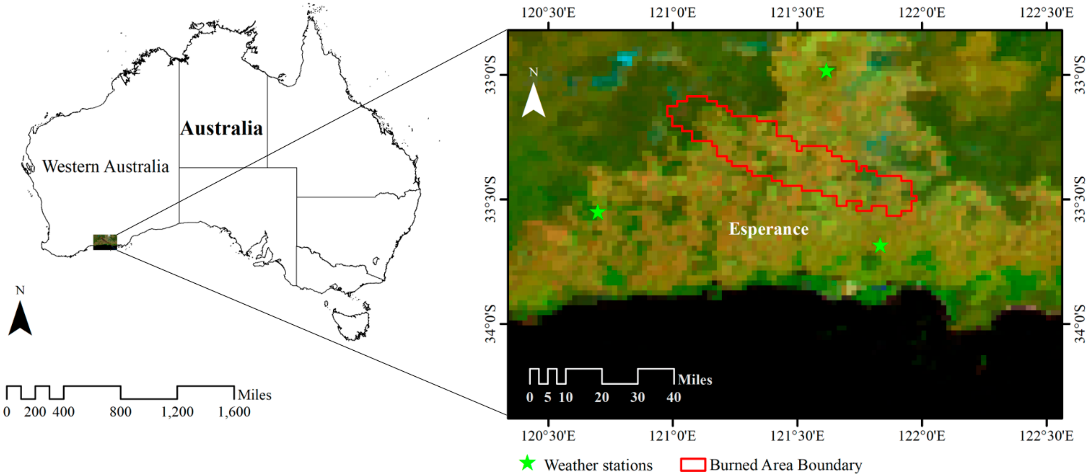
2.1. Study Area
2.2. Himawari-8 Data
2.3. Meteorological Data
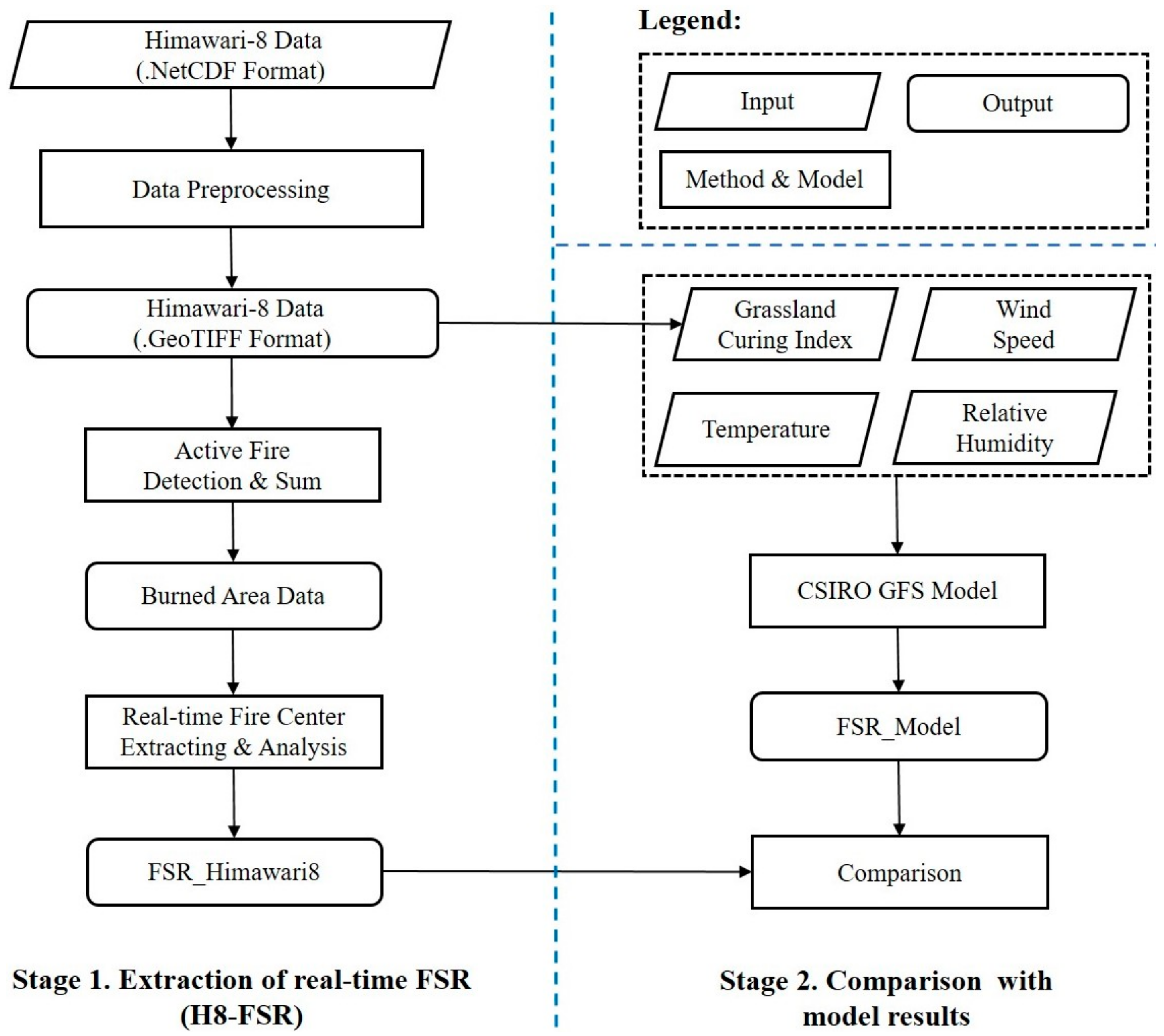
3. Methodology
3.1. Data Preprocessing
3.2. Near Real-Time Burned Area Detection
3.3. Near Real-Time Fire Center Extraction
3.4. Near Real-Time FSR Calculation
3.5. Comparison of Results with the CSIRO GFS Model
4. Results
4.1. Burned Area Variation
4.2. Near Real-Time FSR
5. Discussion
6. Conclusions
Author Contributions
Funding
Acknowledgments
Conflicts of Interest
References
- Ruokolainen, L.; Salo, K. The effect of fire intensity on vegetation succession on a sub-xeric heath during ten years after wildfire. Ann. Bot. Fenn. 2009, 46, 30–42. [Google Scholar] [CrossRef]
- Bowman, D.M.; Balch, J.K.; Artaxo, P.; Bond, W.J.; Carlson, J.M.; Cochrane, M.A.; D’Antonio, C.M.; Defries, R.S.; Doyle, J.C.; Harrison, S.P.; et al. Fire in the earth system. Science 2009, 324, 481–484. [Google Scholar] [CrossRef] [PubMed]
- Chu, T.; Guo, X. Remote sensing techniques in monitoring post-fire effects and patterns of forest recovery in boreal forest regions: A review. Remote Sens. 2013, 6, 470–520. [Google Scholar] [CrossRef]
- Boerner, R.E.J.; Huang, J.; Hart, S.C. Impacts of fire and fire surrogate treatments on forest soil properties: A meta-analytical approach. Ecol. Appl. 2009, 19, 338–358. [Google Scholar] [CrossRef] [PubMed]
- Kilgore, B.M. The ecological role of fire in sierran conifer forests: Its application to national park management. Quat. Res. 1973, 3, 496–513. [Google Scholar] [CrossRef]
- Van der Werf, G.R.; Morton, D.C.; DeFries, R.S.; Olivier, J.G.J.; Kasibhatla, P.S.; Jackson, R.B.; Collatz, G.J.; Randerson, J.T. CO2 emissions from forest loss. Nat. Geosci. 2009, 2, 737–738. [Google Scholar] [CrossRef]
- Van der Werf, G.R.; Randerson, J.T.; Giglio, L.; Collatz, G.J.; Kasibhatla, P.S.; Arellano, A.F. Interannual variability in global biomass burning emissions from 1997 to 2004. Atmos. Chem. Phys. 2006, 6, 3423–3441. [Google Scholar] [CrossRef] [Green Version]
- Kochi, I.; Donovan, G.H.; Champ, P.A.; Loomis, J.B. The economic cost of adverse health effectsfrom wildfire-smoke exposure: A review. Int. J. Wildland Fire 2010, 19, 803–817. [Google Scholar] [CrossRef]
- Hesseln, H.; Loomis, J.B.; Gonzalez-Caban, A.; Alexander, S. Wildfire effects on hiking and biking demand in new mexico: A travel cost study. J. Environ. Manag. 2003, 69, 359–368. [Google Scholar] [CrossRef] [PubMed]
- Richardson, L.A.; Champ, P.A.; Loomis, J.B. The hidden cost of wildfires: Economic valuation of health effects of wildfire smoke exposure in southern california. J. For. Econ. 2012, 18, 14–35. [Google Scholar] [CrossRef]
- Doerr, S.H.; Santin, C. Global trends in wildfire and its impacts: Perceptions versus realities in a changing world. Philos. Trans. R. Soc. Biol. Sci. 2016, 371. [Google Scholar] [CrossRef] [PubMed]
- Johnston, F.H.; Henderson, S.B.; Chen, Y.; Randerson, J.T.; Marlier, M.; Defries, R.S.; Kinney, P.; Bowman, D.M.; Brauer, M. Estimated global mortality attributable to smoke from landscape fires. Environ. Health Perspect. 2012, 120, 695–701. [Google Scholar] [CrossRef] [PubMed]
- Cruz, M.G.; Gould, J.S.; Alexander, M.E.; Sullivan, A.L.; McCaw, W.L.; Matthews, S. Empirical-based models for predicting head-fire rate of spread in australian fuel types. Aust. For. 2015, 78, 118–158. [Google Scholar] [CrossRef]
- Rossa, C.G.; Fernandes, P.M. Fuel-related fire-behaviour relationships for mixed live and dead fuels burned in the laboratory. Can. J. For. Res. 2017, 47, 883–889. [Google Scholar] [CrossRef] [Green Version]
- Cruz, M.G.; Alexander, M.E.; Sullivan, A.L.; Gould, J.S.; Kilinc, M. Assessing improvements in models used to operationally predict wildland fire rate of spread. Environ. Model. Softw. 2018, 105, 54–63. [Google Scholar] [CrossRef]
- Cheney, N.P.; Gould, J.S.; McCaw, W.L.; Anderson, W.R. Predicting fire behaviour in dry eucalypt forest in southern Australia. For. Ecol. Manag. 2012, 280, 120–131. [Google Scholar] [CrossRef]
- Jenkins, M.J.; Page, W.G.; Hebertson, E.G.; Alexander, M.E. Fuels and fire behavior dynamics in bark beetle-attacked forests in western north america and implications for fire management. For. Ecol. Manag. 2012, 275, 23–34. [Google Scholar] [CrossRef]
- Cruz, M.G.; Alexander, M.E. Modelling the rate of fire spread and uncertainty associated with the onset and propagation of crown fires in conifer forest stands. Int. J. Wildland Fire 2017, 26, 413–426. [Google Scholar]
- Benali, A.A.; Pereira, J.M.C. Monitoring and extracting relevant parameters of wild fire spread using remote sensing data. In Proceedings of the Anais XVI Simpósio Brasileiro de Sensoriamento Remoto-SBSR, Foz do Iguaçu, PR, Brasil, 13–18 April 2013. [Google Scholar]
- Gould, J.S.; Sullivan, A.L.; Hurley, R.; Koul, V. Comparison of three methods to quantify the fire spread rate in laboratory experiments. Int. J. Wildland Fire 2017, 26, 877. [Google Scholar] [CrossRef]
- Sullivan, A.L. Wildland surface fire spread modelling, 1990–2007. 1: Physical and quasi-physical models. Int. J. Wildland Fire 2009, 18, 349–368. [Google Scholar] [CrossRef]
- Sullivan, A.L. Wildland surface fire spread modelling, 1990–2007. 2: Empirical and quasi-empirical models. Int. J. Wildland Fire 2009, 18, 369–386. [Google Scholar] [CrossRef]
- Plucinski, M.P.; Sullivan, A.L.; Rucinski, C.J.; Prakash, M. Improving the reliability and utility of operational bushfire behaviour predictions in australian vegetation. Environ. Model. Softw. 2017, 91, 1–12. [Google Scholar] [CrossRef]
- Rothermel, R.C. A Mathematical Model for Predicting Fire Spread in Wildland Fuels; USDA Forest Service Research Paper INT-115; U.S. Department of Agriculture, Forest Service, Intermountain Forest and Range Experiment Station: Ogden, UT, USA, 1972. [Google Scholar]
- Lawson, B.D.; Stocks, B.J.; Alexander, M.E.; Van Wagner, C.E. A system for predicting fire behavior in canadian forests. In Proceedings of the 8th Conference on Fire and Forest Meteorology, Detroit, MI, USA, 29 April–2 May 1985. [Google Scholar]
- McArthur, A.G. Fire Behavior in Eucalypt Forests; Department of National Development, Forestry and Timber Bureau Leaflet: Canberra, Australia, 1967. [Google Scholar]
- Cheney, N.P.; Gould, J.S.; Catchpole, W.R. Prediction of fire spread in grasslands. Int. J. Wildland Fire 1998, 8, 1–13. [Google Scholar] [CrossRef]
- Cruz, M.G.; Alexander, M.E. Uncertainty associated with model predictions of surface and crown fire rates of spread. Environ. Model. Softw. 2013, 47, 16–28. [Google Scholar] [CrossRef]
- Linn, R.; Reisner, J.; Colman, J.J.; Winterkamp, J. Studying wildfire behavior using firetec. Int. J. Wildland Fire 2002, 11, 233. [Google Scholar] [CrossRef]
- Lymberopoulos, N.; Tryfonopoulos, T.; Lockwood, F. The study of small and meso-scale wind field-forest fire interaction and buoyancy effects using the aiolos-f simulator. In Proceedings of the III International Conference on Forest Fire Research, 14th Conference on Fire and Forest Meteorology, Luso, Portugal, 16–20 November 1998. [Google Scholar]
- Morvan, D.; Larini, M. Modeling of one dimensional fire spread in pine needles with opposing air flow. Combust. Sci. Technol. 2001, 164, 37–64. [Google Scholar] [CrossRef]
- Mell, W.; Jenkins, M.A.; Gould, J.; Cheney, P. A physics-based approach to modelling grassland fires. Int. J. Wildland Fire 2007, 16, 1–22. [Google Scholar] [CrossRef]
- Cruz, M.G.; Kidnie, S.; Matthews, S.; Hurley, R.J.; Slijepcevic, A.; Nichols, D.; Gould, J.S. Evaluation of the predictive capacity of dead fuel moisture models for eastern australia grasslands. Int. J. Wildland Fire 2016, 25, 995–1001. [Google Scholar] [CrossRef]
- Stow, D.A.; Riggan, P.J.; Storey, E.J.; Coulter, L.L. Measuring fire spread rates from repeat pass airborne thermal infrared imagery. Remote Sens. Lett. 2014, 5, 803–812. [Google Scholar] [CrossRef]
- Loboda, T.V.; Csiszar, I.A. Reconstruction of fire spread within wildland fire events in northern eurasia from the modis active fire product. Glob. Planet. Chang. 2007, 56, 258–273. [Google Scholar] [CrossRef]
- Sifakis, N.I.; Iossifidis, C.; Kontoes, C.; Keramitsoglou, I. Wildfire detection and tracking over greece using msg-seviri satellite data. Remote Sens. 2011, 3, 524–538. [Google Scholar] [CrossRef]
- Hally, B.; Wallace, L.; Reinke, K.; Jones, S. Assessment of the utility of the advanced himawari imager to detect active fire over Australia. In Proceedings of the XXIII ISPRS Congress, Prague, Czech Republic, 12–19 July 2016. [Google Scholar]
- Zhang, X.; Kondragunta, S.; Ram, J.; Schmidt, C.; Huang, H.-C. Near-real-time global biomass burning emissions product from geostationary satellite constellation. J. Geophys. Res. Atmos. 2012, 117, 1–18. [Google Scholar] [CrossRef]
- Zhang, X.; Kondragunta, S. Temporal and spatial variability in biomass burned areas across the USA derived from the goes fire product. Remote Sens. Environ. 2008, 112, 2886–2897. [Google Scholar] [CrossRef]
- Calle, A.; Casanova, J.L.; Romo, A. Fire detection and monitoring using msg spinning enhanced visible and infrared imager (seviri) data. J.Geophys. Res. Biogeosci. 2006, 111. [Google Scholar] [CrossRef]
- Laneve, G.; Castronuovo, M.M.; Cadau, E.G. Continuous monitoring of forest fires in the mediterranean area using msg. IEEE Trans. Geosci. Remote Sens. 2006, 44, 2761–2768. [Google Scholar] [CrossRef]
- Kim, G.; Kim, D.-S.; Park, K.-W.; Cho, J.; Han, K.-S.; Lee, Y.-W. Detecting wildfires with the korean geostationary meteorological satellite. Remote Sens. Lett. 2014, 5, 19–26. [Google Scholar] [CrossRef]
- Da, C. Preliminary assessment of the advanced himawari imager (ahi) measurement onboard himawari-8 geostationary satellite. Remote Sens. Lett. 2015, 6, 637–646. [Google Scholar] [CrossRef]
- Fatkhuroyan; Wati, T.; Panjaitan, A. Forest fires detection in indonesia using satellite himawari-8 (case study: Sumatera and kalimantan on august-october 2015). IOP Conf. Ser. Earth Environ. Sci. 2017, 54. [Google Scholar] [CrossRef]
- Sataid Software. Available online: https://www.data.jma.go.jp/mscweb/en/VRL/sataid/program.html (accessed on 16 October 2018).
- Xu, G.; Zhong, X. Real-time wildfire detection and tracking in australia using geostationary satellite: Himawari-8. Remote Sens. Lett. 2017, 8, 1052–1061. [Google Scholar] [CrossRef]
- Xu, W.; Wooster, M.J.; Kaneko, T.; He, J.; Zhang, T.; Fisher, D. Major advances in geostationary fire radiative power (frp) retrieval over asia and australia stemming from use of himarawi-8 ahi. Remote Sens. Environ. 2017, 193, 138–149. [Google Scholar] [CrossRef]
- Wickramasinghe, C.; Jones, S.; Reinke, K.; Wallace, L. Development of a multi-spatial resolution approach to the surveillance of active fire lines using himawari-8. Remote Sens. 2016, 8, 932. [Google Scholar] [CrossRef]
- Bessho, K.; Date, K.; Hayashi, M.; Ikeda, A.; Imai, T.; Inoue, H.; Kumagai, Y.; Miyakawa, T.; Murata, H.; Ohno, T.; et al. An introduction to himawari-8/9-japan’s new-generation geostationary meteorological satellites. J. Meteorol. Soc. Jpn. 2016, 94, 151–183. [Google Scholar] [CrossRef]
- JAXA Website. Available online: http://www.eorc.jaxa.jp/ptree/ (accessed on 16 October 2018).
- Australian Bureau of Meteorology Website. Available online: http://reg.bom.gov.au (accessed on 16 October 2018).
- Giglio, L.; Schroeder, W.; Justice, C.O. The collection 6 modis active fire detection algorithm and fire products. Remote Sens. Environ. 2016, 178, 31–41. [Google Scholar] [CrossRef] [PubMed]
- Rocchini, D.; Cateni, C. On the measure of spatial centroid in geography. Asian J. Inf. Technol. 2006, 5, 729–731. [Google Scholar]
- Bourke, P. Calculating the Area and Centroid of a Polygon. Available online: https://www.seas.upenn.edu/~sys502/extra_materials/Polygon%20Area%20and%20Centroid.pdf (accessed on 16 October 2018).
- Deakin, R.E.; Bird, S.C.; Grenfell, R.I. The centroid? Where would you like it to be be? Cartography 2002, 31, 153–167. [Google Scholar] [CrossRef]
- De Smith, M.J.; Goodchild, M.F.; Longley, P. Geospatial Analysis: A Comprehensive Guide to Principles, Techniques and Software Tools; Troubador Publishing Ltd.: Leicester, UK, 2007. [Google Scholar]
- Richards, G.D. A general mathematical framework for modeling two-dimensional wildland fire spread. Int. J. Wildland Fire 1995, 5, 63–72. [Google Scholar] [CrossRef]
- Rios, O.; Jahn, W.; Rein, G. Forecasting wind-driven wildfires using an inverse modelling approach. Nat. Hazards Earth Syst. Sci. 2014, 14, 1491–1503. [Google Scholar] [CrossRef] [Green Version]
- R software v3.4.1. Available online: https://cran.r-project.org/bin/windows/base/old/3.4.1/ (accessed on 16 October 2018).
- Glasa, J.; Halada, L. On elliptical model for forest fire spread modeling and simulation. Math. Comput. Simul. 2008, 78, 76–88. [Google Scholar] [CrossRef]
- Anderson, D.H.; Catchpole, E.A.; De Mestre, N.J.; Parkes, T. Modelling the spread of grass fires. J. Aust. Math. Soc. Ser. B Appl. Math. 1982, 23, 451–466. [Google Scholar] [CrossRef]
- Richards, G.D. An elliptical growth model of forest fire fronts and its numerical solution. Int. J. Numer. Methods Eng. 1990, 30, 1163–1179. [Google Scholar] [CrossRef]
- Richards, G.D. The properties of elliptical wildfire growth for time dependent fuel and meteorological conditions. Combust. Sci. Technol. 1993, 95, 357–383. [Google Scholar] [CrossRef]
- R software v3.4.1. Available online: https://www7.ncdc.noaa.gov/climvis/help_wind.html (accessed on 16 October 2018).
- Cruz, M.G.; Gould, J.S.; Alexander, M.E.; Sullivan, A.L.; McCaw, W.L.; Matthews, S. A Guide to Rate of Fire Spread Models for Australian Vegetation; Australasian Fire and Emergency Service Authorities Council Limited and Commonwealth Scientific and Industrial Research Organisation: Cabberra, ACT, Australia, 2015. [Google Scholar]
- Cruz, M.G.; Gould, J.S.; Kidnie, S.; Bessell, R.; Nichols, D.; Slijepcevic, A. Effects of curing on grassfires: Ii. Effect of grass senescence on the rate of fire spread. Int. J. Wildland Fire 2015, 24, 838–848. [Google Scholar] [CrossRef]
- Martin, D.; Chen, T.; Nichols, D.; Bessell, R.; Kidnie, S.; Alexander, J. Integrating ground and satellite-based observations to determine the degree of grassland curing. Int. J. Wildland Fire 2015, 24, 329–339. [Google Scholar] [CrossRef]
- Newnham, G.J.; Grant, I.F.; Martin, D.N.; Anderson, S.A. Improved Methods for Assessment and Prediction of Grassland Curing. Available online: http://www.bushfirecrc.com/publications/citation/bf-2555 (accessed on 16 October 2018).
- Willmott, C.J. Some comments on the evaluation of model performance. Bull. Am. Meteorol. Soc. 1982, 63, 1309–1313. [Google Scholar] [CrossRef]
- Sullivan, A.L. Grassland fire management in future climate. Adv. Agron. 2010, 106, 173–208. [Google Scholar]
- Pyne, S.J.; Andrews, P.L.; Laven, R.D. Introduction to Wildland Fire; John Wiley and Sons: New York, NY, USA, 1996. [Google Scholar]
- Rossa, C.G. The effect of fuel moisture content on the spread rate of forest fires in the absence of wind or slope. Int. J. Wildland Fire 2017, 26, 24–31. [Google Scholar] [CrossRef]
- Rossa, C.G.; Fernandes, P.M. Short communication: On the effect of live fuel moisture content on fire-spread rate. For. Syst. 2018, 26, eSC08. [Google Scholar] [CrossRef]
- Dasgupta, S.; Qu, J.; Hao, X.; Bhoi, S. Evaluating remotely sensed live fuel moisture estimations for fire behavior predictions in georgia, USA. Remote Sens. Environ. 2007, 108, 138–150. [Google Scholar] [CrossRef]
- Quan, X.; He, B.; Yebra, M.; Yin, C.; Liao, Z.; Li, X. Retrieval of forest fuel moisture content using a coupled radiative transfer model. Environ. Model. Softw. 2017, 95, 290–302. [Google Scholar] [CrossRef]
- Quan, X.W.; He, B.B.; Li, X.; Tang, Z. Estimation of grassland live fuel moisture content from ratio of canopy water content and foliage dry biomass. IEEE Geosci. Remote Sens. Lett. 2015, 12, 1903–1907. [Google Scholar] [CrossRef]
- Yebra, M.; Quan, X.; Riaño, D.; Rozas Larraondo, P.; van Dijk, A.I.J.M.; Cary, G.J. A fuel moisture content and flammability monitoring methodology for continental australia based on optical remote sensing. Remote Sens. Environ. 2018, 212, 260–272. [Google Scholar] [CrossRef]
- Yebra, M.; Dennison, P.E.; Chuvieco, E.; Riaño, D.; Zylstra, P.; Hunt, E.R.; Danson, F.M.; Qi, Y.; Jurdao, S. A global review of remote sensing of live fuel moisture content for fire danger assessment: Moving towards operational products. Remote Sens. Environ. 2013, 136, 455–468. [Google Scholar] [CrossRef]
- Quan, X.; He, B.; Yebra, M.; Yin, C.; Liao, Z.; Zhang, X.; Li, X. A radiative transfer model-based method for the estimation of grassland aboveground biomass. Int. J. Appl. Earth Obs. Geoinf. 2017, 54, 159–168. [Google Scholar] [CrossRef]
- Jiménez, P.A.; Dudhia, J. On the ability of the wrf model to reproduce the surface wind direction over complex terrain. J. Appl. Meteorol. Climatol. 2013, 52, 1610–1617. [Google Scholar] [CrossRef]
- Mahrt, L. Surface wind direction variability. J. Appl. Meteorol. Climatol. 2011, 50, 144–152. [Google Scholar] [CrossRef]


| Difference | △(°) | ||||
|---|---|---|---|---|---|
| 0–5 | 5–10 | 10–15 | 15–22.5 | >22.5 | |
| Number of time periods | 13 | 7 | 6 | 4 | 6 |
| % of Total | 36.11 | 19.44 | 16.67 | 11.16 | 16.67 |
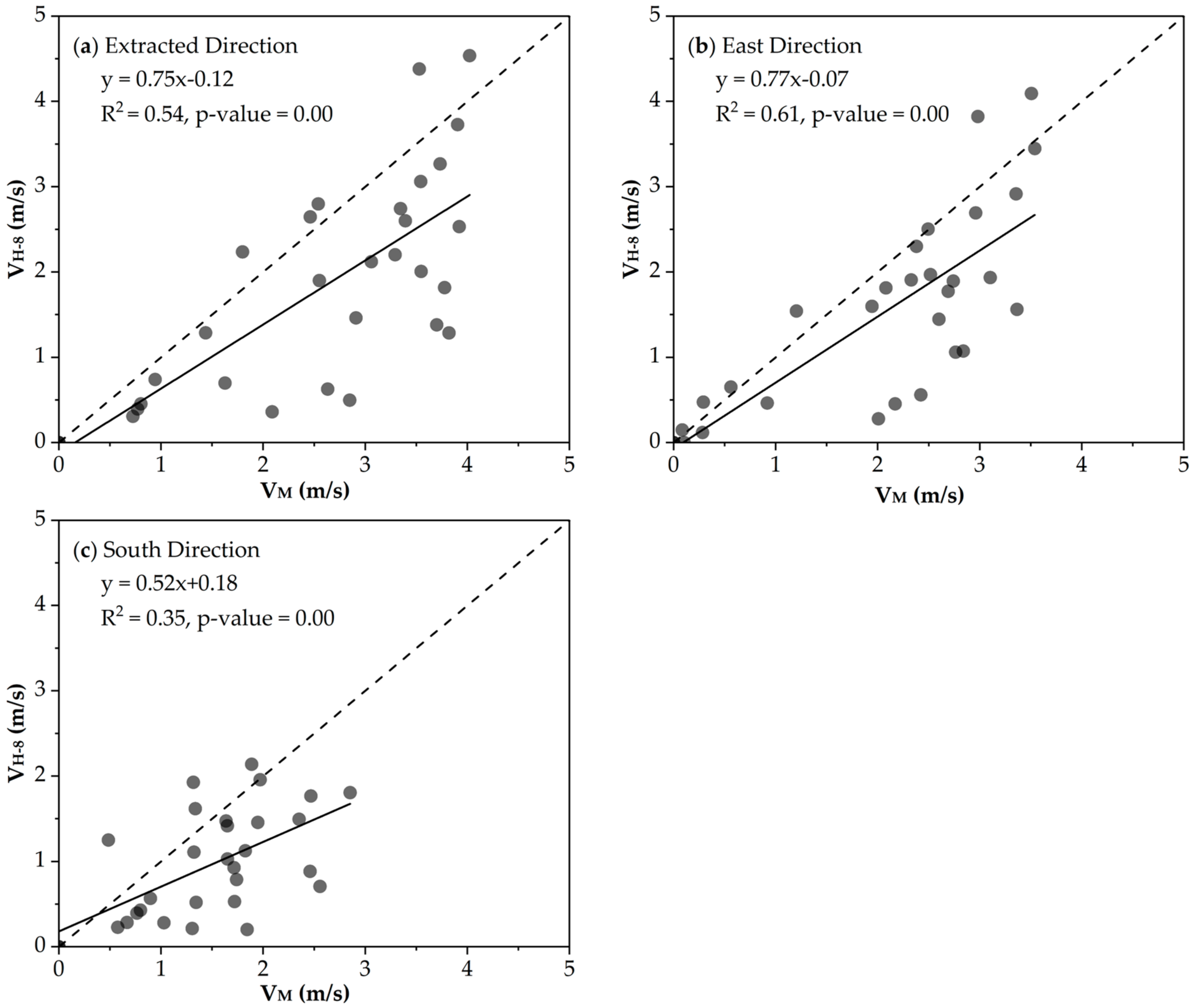
| Extracted Direction | East Direction | South Direction | |
|---|---|---|---|
| MBE (m/s) | −0.75 | −0.52 | −0.52 |
| MAPE (%) | 33.20 | 35.53 | 43.33 |
| RMSE (m/s) | 1.17 | 0.92 | 0.80 |
| R2 | 0.54 *** | 0.61 *** | 0.35 *** |
© 2018 by the authors. Licensee MDPI, Basel, Switzerland. This article is an open access article distributed under the terms and conditions of the Creative Commons Attribution (CC BY) license (http://creativecommons.org/licenses/by/4.0/).
Share and Cite
Liu, X.; He, B.; Quan, X.; Yebra, M.; Qiu, S.; Yin, C.; Liao, Z.; Zhang, H. Near Real-Time Extracting Wildfire Spread Rate from Himawari-8 Satellite Data. Remote Sens. 2018, 10, 1654. https://0-doi-org.brum.beds.ac.uk/10.3390/rs10101654
Liu X, He B, Quan X, Yebra M, Qiu S, Yin C, Liao Z, Zhang H. Near Real-Time Extracting Wildfire Spread Rate from Himawari-8 Satellite Data. Remote Sensing. 2018; 10(10):1654. https://0-doi-org.brum.beds.ac.uk/10.3390/rs10101654
Chicago/Turabian StyleLiu, Xiangzhuo, Binbin He, Xingwen Quan, Marta Yebra, Shi Qiu, Changming Yin, Zhanmang Liao, and Hongguo Zhang. 2018. "Near Real-Time Extracting Wildfire Spread Rate from Himawari-8 Satellite Data" Remote Sensing 10, no. 10: 1654. https://0-doi-org.brum.beds.ac.uk/10.3390/rs10101654