Article

Mapping Crop Residue and Tillage Intensity Using WorldView-3 Satellite Shortwave Infrared Residue Indices

1
U.S. Geological Survey, Lower Mississippi-Gulf Water Science Center, Beltsville, MD 20705, USA
2
Department of Earth and Atmospheric Sciences, The City College of New York, City University of New York, New York, NY 10031, USA
3
U.S. Department of Agriculture, Agricultural Research Service, Hydrology and Remote Sensing Laboratory, Beltsville, MD 20705, USA
4
U.S. Geological Survey, Eastern Geographic Science Center; Reston, VA 20192, USA
5
School of Agricultural Engineering, Dept. Agricultural Production, CEIGRAM, Universidad Politécnica de Madrid, 28040 Madrid, Spain
*
Author to whom correspondence should be addressed.
Current address: In-Q-Tel, CosmiQ Works, Arlington, VA 22003, USA.
Remote Sens. 2018, 10(10), 1657; https://0-doi-org.brum.beds.ac.uk/10.3390/rs10101657
Submission received: 23 August 2018 / Revised: 20 September 2018 / Accepted: 9 October 2018 / Published: 18 October 2018
(This article belongs to the Special Issue Quantitative Remote Sensing of Land Surface Variables)

Abstract

:
Crop residues serve many important functions in agricultural conservation including preserving soil moisture, building soil organic carbon, and preventing erosion. Percent crop residue cover on a field surface reflects the outcome of tillage intensity and crop management practices. Previous studies using proximal hyperspectral remote sensing have demonstrated accurate measurement of percent residue cover using residue indices that characterize cellulose and lignin absorption features found between 2100 nm and 2300 nm in the shortwave infrared (SWIR) region of the electromagnetic spectrum. The 2014 launch of the WorldView-3 (WV3) satellite has now provided a space-borne platform for the collection of narrow band SWIR reflectance imagery capable of measuring these cellulose and lignin absorption features. In this study, WorldView-3 SWIR imagery (14 May 2015) was acquired over farmland on the Eastern Shore of Chesapeake Bay (Maryland, USA), was converted to surface reflectance, and eight different SWIR reflectance indices were calculated. On-farm photographic sampling was used to measure percent residue cover at a total of 174 locations in 10 agricultural fields, ranging from plow-till to continuous no-till management, and these in situ measurements were used to develop percent residue cover prediction models from the SWIR indices using both polynomial and linear least squares regressions. Analysis was limited to agricultural fields with minimal green vegetation (Normalized Difference Vegetation Index < 0.3) due to expected interference of vegetation with the SWIR indices. In the resulting residue prediction models, spectrally narrow residue indices including the Shortwave Infrared Normalized Difference Residue Index (SINDRI) and the Lignin Cellulose Absorption Index (LCA) were determined to be more accurate than spectrally broad Landsat-compatible indices such as the Normalized Difference Tillage Index (NDTI), as determined by respective R2 values of 0.94, 0.92, and 0.84 and respective residual mean squared errors (RMSE) of 7.15, 8.40, and 12.00. Additionally, SINDRI and LCA were more resistant to interference from low levels of green vegetation. The model with the highest correlation (2nd order polynomial SINDRI, R2 = 0.94) was used to convert the SWIR imagery into a map of crop residue cover for non-vegetated agricultural fields throughout the imagery extent, describing the distribution of tillage intensity within the farm landscape. WorldView-3 satellite imagery provides spectrally narrow SWIR reflectance measurements that show utility for a robust mapping of crop residue cover.

Graphical Abstract

1. Introduction

1.1. Crop Residue and Conservation Tillage

Crop residue is plant litter (non-photosynthetic vegetation) that accumulates on the surface of agricultural fields, generally after harvest has occurred and crops have senesced. The residues cover the soil surface with a mulch layer that plays an important role in soil conservation by reducing both water-based and wind-based erosion [1]. Additionally, crop residue can preserve soil moisture, reduce evaporation, inhibit the germination of weeds, increase soil organic carbon, and support healthy soil ecosystems [2,3]. The amount of crop residue cover is directly linked to crop system management, responding to tillage practices, crop rotations, and harvest methods.
Reducing tillage intensity, with corresponding increases in crop residue cover, can increase soil water retention and help to control soil erosion, mitigating nutrient losses in runoff [4]. The diversity of tillage practices employed by farmers (e.g., plow-till, chisel plow, disking, zone till, vertical till, no-till) reflects the continuing evolution of agricultural mechanization, and results in a broad spectrum of crop residue cover outcomes [5]. High-residue crop management practices are key components of conservation agriculture, and are crucial to promote sustainable cropping systems, complementing additional practices such as reduced chemical usage, improved nutrient management, and diversified crop rotations [1,6].

1.2. Chesapeake Bay Setting

Prevention of erosion and runoff, and retention of agricultural nutrients on farmland, are of great importance in the Chesapeake Bay watershed, which has been subject to extensive anthropogenic ecological stressors, including significant impacts from farming [7]. Elevated nutrient and sediment levels have plagued the Chesapeake Bay for several decades, reducing the extent of submerged aquatic vegetation and creating algal blooms and hypoxic zones in the estuary [8]. Conservation management practices, including the use of conservation tillage and winter cover crops, have played pivotal roles in reducing nutrient inputs to the estuary [9]. Therefore, management practices that maintain crop residue on the field surface are promoted by Chesapeake Bay restoration efforts. To verify and promote the implementation of effective conservation tillage practices, there is a need to map and identify the amount and distribution of crop residue in the working farm landscape.
The Chesapeake Bay Program Partnership has defined four categories of tillage intensity for use in their watershed model [10]: conventional tillage (<15% cover); low residue tillage (15–30% cover); conservation tillage (30–60% cover); and high residue tillage (>60% cover). These classes are similar to those used nationally by the Conservation Technology Information Center (CTIC: https://www.ctic.org/resourcedisplay/322/), with the addition of the high residue tillage category. The classes with lower percent cover are associated with a higher risk of erosion and sediment transport, due to increased dislodgement of soil particles by rainfall and wind. Greater than 30% residue cover is expected to control roughly 65% of soil erosion, depending on soil type, slope, and local conditions, while >60% cover is expected to control >90% of erosion [11,12]. Residue cover outcomes resulting from agronomic management depend on many factors, such as crop residue type (species, size, durability, lignification), climate (moisture and temperature), and tillage intensity.

1.3. Ground-Based Measurement of Crop Residue Cover

Soil tillage intensity is typically characterized by the fraction of soil covered by crop residues in the late spring, shortly after tillage is complete and summer crops have been planted (https://www.ctic.org/resourcedisplay/255/). At that time there is a brief window of opportunity for the measurement of crop residue cover before crop vegetation covers the soil surface. Various ground-based methods exist for assessing the amount of residue cover on agricultural fields [13,14], including roadside surveys, in-field photography, and line-point transects. Each of these methods has its own merits, but the challenges associated with assessing crop residue cover in many fields in a timely manner have been highlighted by various researchers [15,16,17,18,19].
Roadside surveys of crop residue cover are made by driving a route through an agricultural area, stopping at intervals, and visually estimating the amount of crop residue cover in fields. The CTIC compiles annual county-level assessments of soil tillage intensity using roadside survey methods (https://www.ctic.org/resourcedisplay/255/). Roadside surveys are time-effective but are often hampered by only observing field edges near the road, which may not be representative of the whole field, and by the oblique viewing angle. The roadside surveys are therefore somewhat subjective and sometimes tend to overestimate crop residue cover in fields with <30% residue cover and underestimate cover for fields with >30% residue cover [16,19].
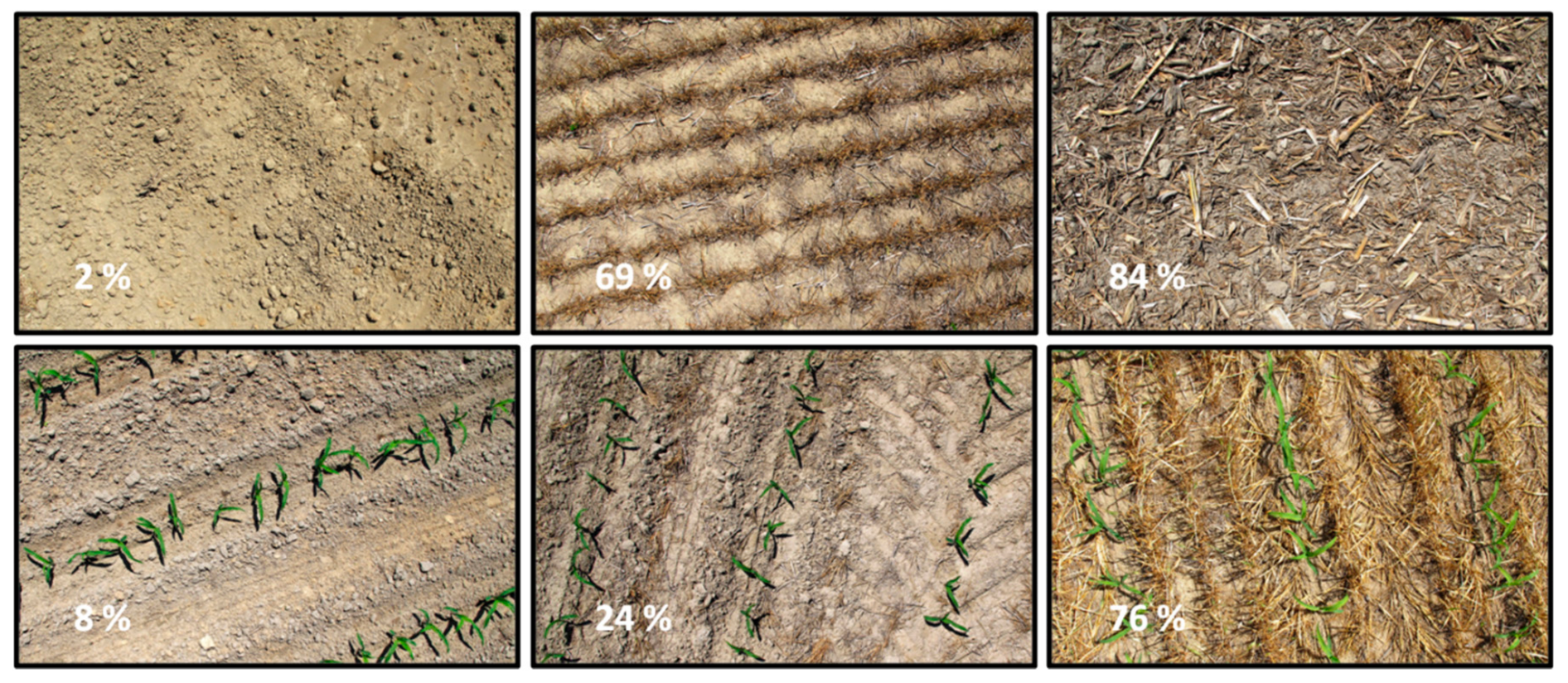
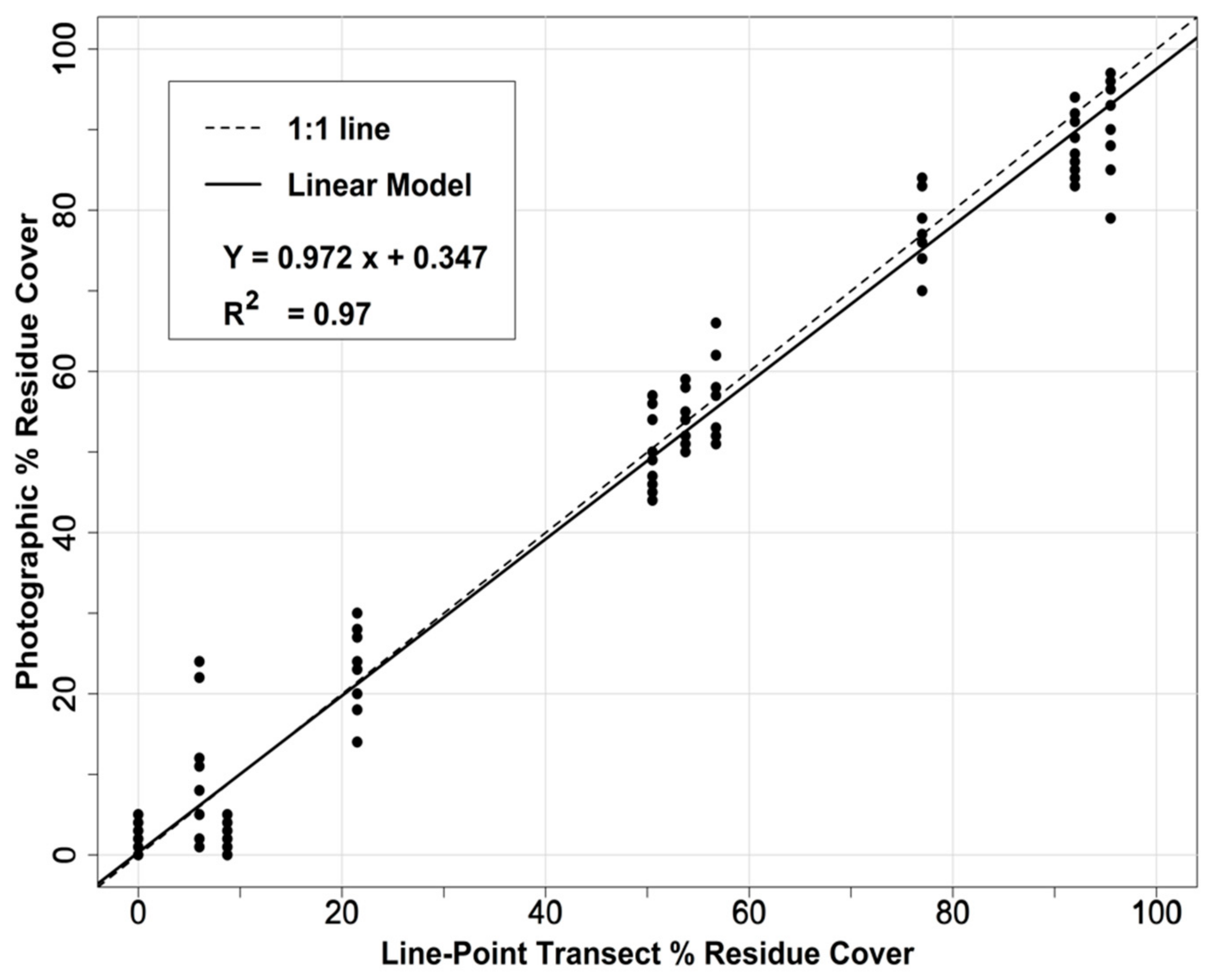
Photographic methods consist of acquiring proximal vertical photographs or digital images of the field surface and estimating the fraction of the soil surface covered by crop residue. Methods include using software (e.g., SamplePoint [20]) to overlay a digital grid of crosshairs on each image and visually determining the number of crosshairs that intersect green vegetation, crop residue, or soil. Accuracy depends on the spatial resolution of the images, the contrast between the soil and the crop residue in each image, the number of crosshairs used, and the skill of the observer. In-field photography can be acquired in a time-effective and accurate manner, but requires access to the fields, and the post-processing to determine percent ground cover can be labor intensive.
The line-point transect method uses a string with small equally spaced markers extended over the field surface, and the observer counts the number of markers that intercept crop residue, green vegetation, or soil. Accuracy depends on the length of the line, the number of markers, and the skill of the observer. The line-point transect method used by the U.S. Department of Agriculture (USDA) Natural Resources Conservation Service (NRCS) typically has 100 1-cm markers evenly spaced along a 15-m string [21]. In-field line-point transect surveys have been demonstrated as being very accurate but are also time consuming to conduct, and do not work well with standing residue.
In contrast to these ground-based methods for measuring crop residue cover, remote sensing from airborne or satellite-based platforms has the potential to offer a rapid and accurate assessment of crop residue cover over large areas in a timely and cost-effective manner, if current limitations can be overcome [22]. Remote sensing, under optimal circumstances, can provide synoptic observations of field residue conditions that are unparalleled by ground-based surveys in terms of both spatial extent and detail of observations.

1.4. Remote Sensing of Crop Residue

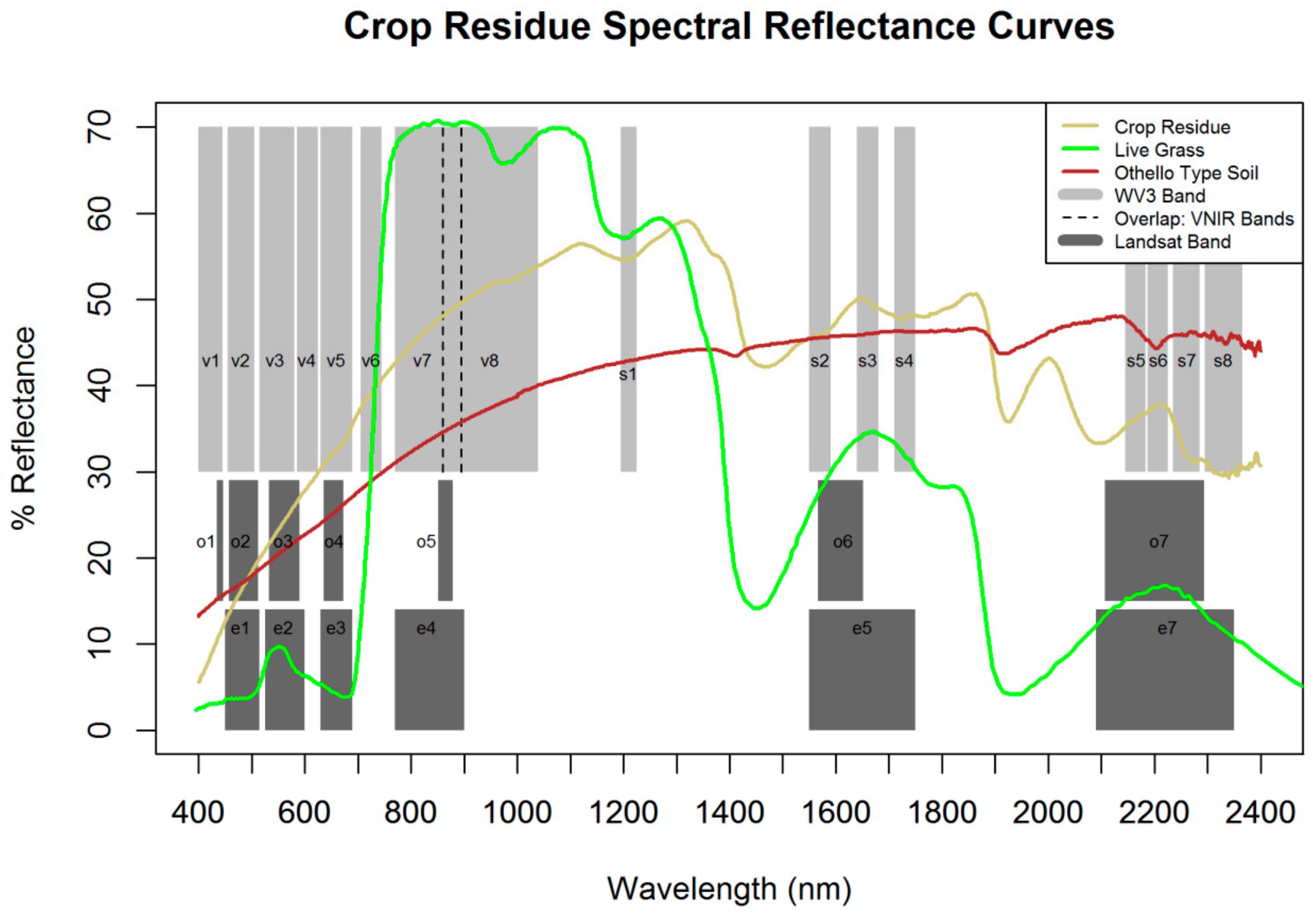
Crop residues have unique spectral absorption features that allow them to be discriminated from soils and vegetation based on their reflectance spectra. They are largely composed of cellulose and lignin, which exhibit absorption features near 2100 nm and 2300 nm [23,24,25,26]. Additionally, crop residues tend to have a general decrease in spectral reflectance from 1600 nm to 2300 nm, in contrast to soils for which spectral reflectance remains relatively constant from 1600 to 2300 nm. These differences in spectral reflectance can be used to generate spectral indices that distinguish soil from crop residue [27,28].
Daughtry et al. [24,29] showed that the Cellulose Absorption Index (CAI), which measures the 2100 nm cellulose absorption feature, was very accurate in determining percent residue cover and for distinguishing crop residue from other types of ground cover. However, this index relies on changes in reflectance within relatively narrow spectral bands (<100 nm) that can only be computed using reflectance data from hyperspectral instruments. The Hyperion sensor aboard the Earth Observing−1 satellite provided space-borne hyperspectral imagery that was used by Bannari et al. [30] to map crop residue, but that instrument was deactivated in 2017 and hyperspectral imagery is currently only available on airborne or proximal platforms. While space-borne hyperspectral sensors are limited in availability and operation, various indices have been developed for mapping crop residue using multispectral satellite imagery [22,27,31], relying on advanced multispectral imagers (i.e., Advanced Spaceborne Thermal Emission and Reflection Radiometer (ASTER), WorldView-3 [32]) as well as broadband multispectral imagers (i.e., Landsat family, Sentinel-2)
The broadband multispectral satellites provide global coverage, and previous studies have shown success using indices relying on a few relatively broad spectral bands for mapping residue cover at regional scales [18,19,33,34,35,
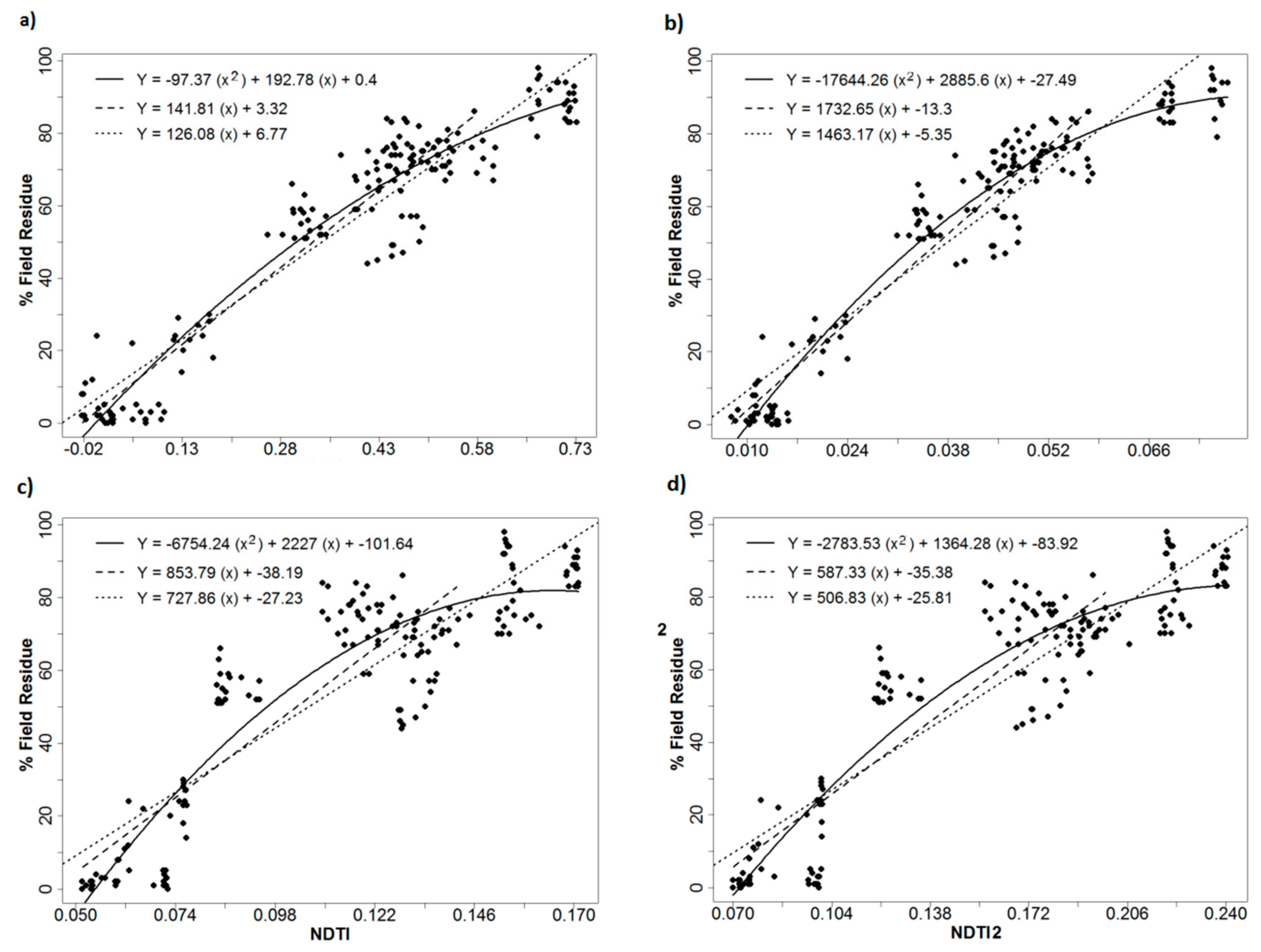
36]. In most cases, the Normalized Difference Tillage Index (NDTI) [34] was demonstrated to be the best of the Landsat-based tillage indices for estimating residue cover, exploiting the difference in reflectance between the two Landsat shortwave infra-red (SWIR) bands centered near 1600 nm and 2300 nm. However, the Landsat-compatible crop residue indices are dependent on spectrally broad contrasts, which can be strongly influenced by crop residue age and condition, moisture content, soil brightness, and the presence of green vegetation [22,37], which limits their effectiveness.
The WorldView-3 (WV3) satellite, launched on August 2014, is now providing advanced multispectral imagery in 16 bands ranging from 400–2500 nm [38]. This includes eight comparatively narrow SWIR bands, and eight bands in the visible near infrared (VNIR). Four of the SWIR bands are spectrally similar to the SWIR bands employed by the ASTER satellite (
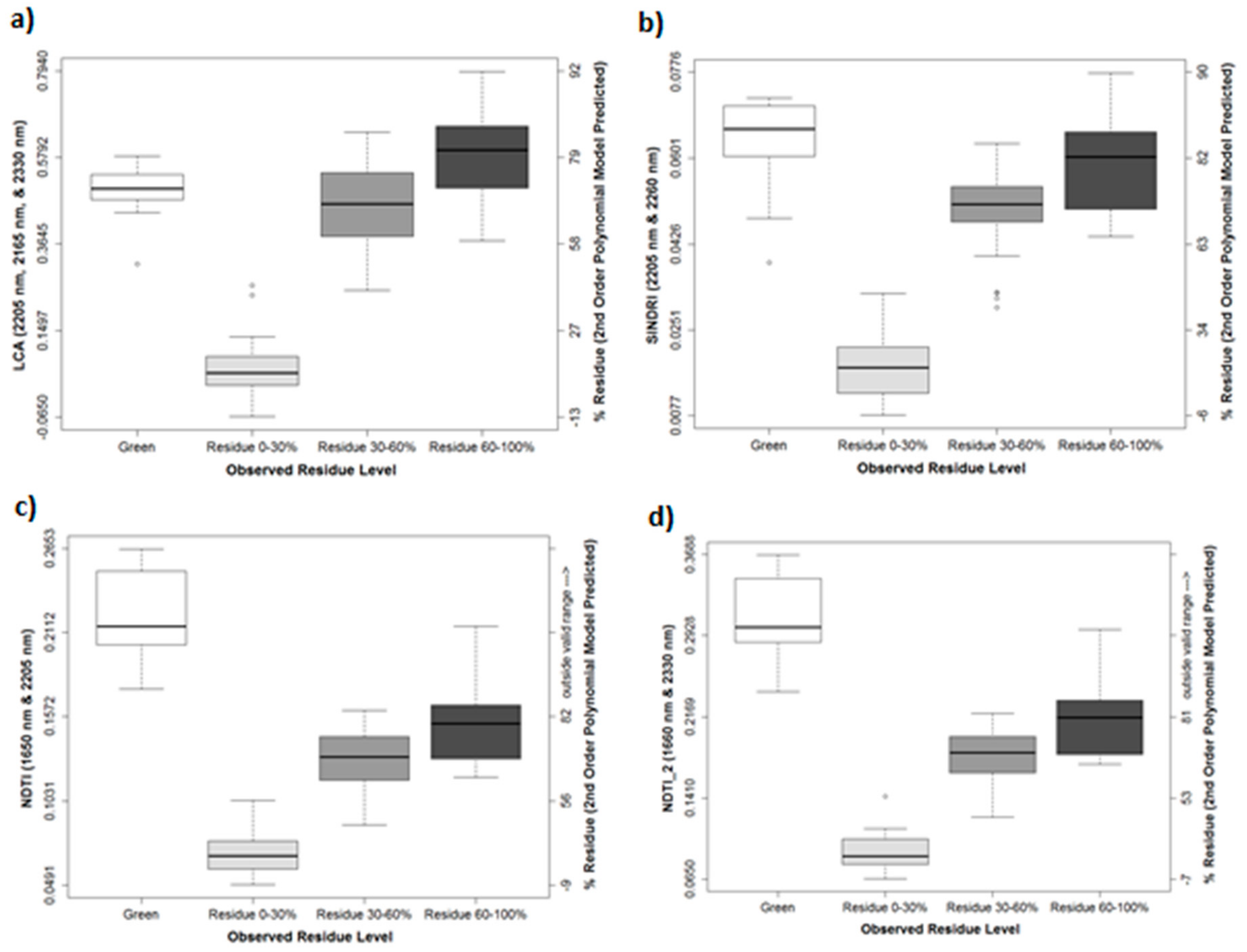
https://asterweb.jpl.nasa.gov/data.asp). The ASTER bands have been used with success to compute advanced multispectral residue indices such as the Lignin Cellulose Absorption Index (LCA) and the Shortwave Infrared Normalized Difference Residue Index (SINDRI) [39,40]. These indices, calculated from the spectrally narrow SWIR bands of ASTER/WV3, have been shown to be more effective at measuring residue cover than indices derived from the spectrally broad SWIR bands employed by Landsat or Sentinel-2 due to the more precise measurement of cellulose and lignin absorption features [37,41]. Although the SWIR instrument of ASTER failed in 2008, WV3 has built upon the ASTER heritage by including additional SWIR bands and higher spatial resolution imagery, enabling the calculation of additional SWIR-based indices suitable for the detection of crop residue cover. The WV3 satellite shows the potential of advanced multispectral imagers to overcome current limitations of remote sensing of crop residue cover and tillage intensity, and to achieve reliable residue cover assessment at the landscape scale [22,42].
Residue decomposition stage, water content, and the presence of green vegetation can impact the accuracy of crop residue characterization using spectral indices. Soil and residue water content can have a strong impact on residue cover estimation [37,43,44]. Increasing moisture content reduces reflectance from the visible to the shortwave infrared and attenuates reflectance features, sometimes resulting in the overestimation of residue cover by spectral residue indices [44]. All residue indices are sensitive to variable moisture conditions, but SINDRI proved more robust than NDTI when no correction for moisture was applied [37]. Similarly, residue decomposition was shown to affect all SWIR residue indices [45], but the narrow band SWIR indices (SINDRI, LCA) were less affected than the broadband indices (NDTI). The presence of green vegetation can physically obscure crop residues, and can also attenuate residue absorption features due to the high water content of green vegetation [22]. Previous studies have dealt with this issue by limiting residue measurement to areas with minimal green vegetation, as indicated by Normalized Difference Vegetation Index (NDVI) values <0.3 [24,40].
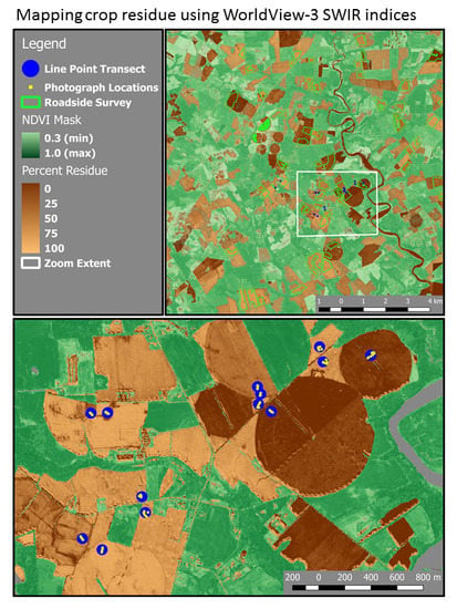
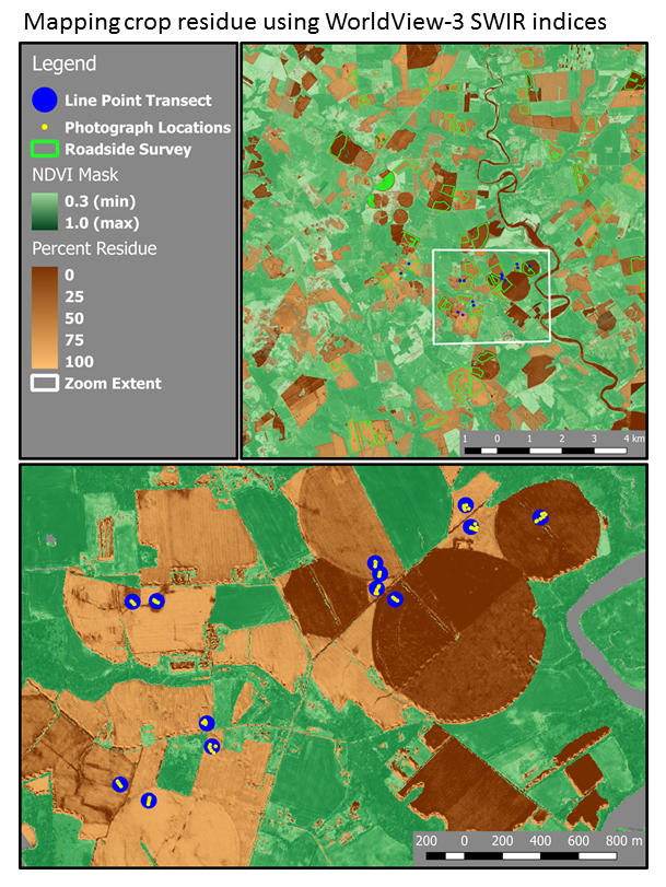
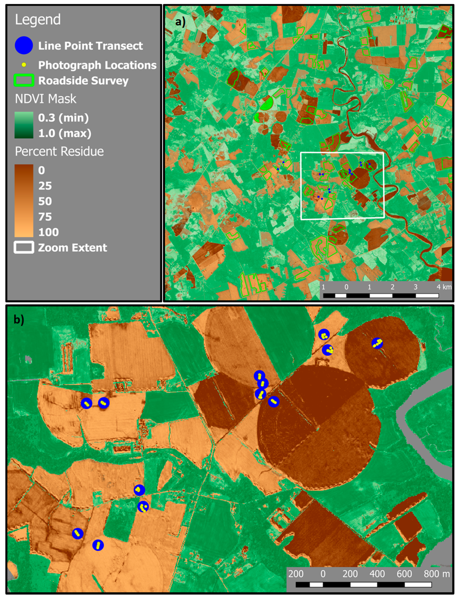
Our objective was to estimate crop residue cover and classify soil tillage intensity using remotely sensed data from the recently launched advanced multispectral satellite, WorldView-3. Various SWIR spectral indices were compared with in situ measurements of crop residue cover, and maps of residue cover on non-vegetated agricultural fields were produced, with a focus on evaluating the potential for using satellite remote sensing technology to quantify the extent and distribution of crop residue cover on agricultural fields of eastern Maryland, USA.

2. Materials and Methods

2.1. Site Location

This study was conducted on a farm located within the Choptank River watershed, on the Eastern Shore of the Chesapeake Bay, Maryland, USA (Figure 1). The farm grows a variety of grain, legume, and vegetable crops, including maize (Zea mays L.), soybean (Glycine max L.), wheat (Triticum aestivum L.), barley (Hordeum vulgare L.), peas (Pisum sativum L.), and cucumbers (Cucumis sativus L.). The fields are managed with a variety of tillage implements ranging from no-till to moldboard plow, resulting in a large range of crop residue cover in the spring season. The majority soil type on the farm is Hambrook silt loam (well-drained, fine-loamy, siliceous, semiactive, mesic, Typic Hapludult (https://soilseries.sc.egov.usda.gov/OSD_Docs/H/HAMBROOK.html)). The regional average annual temperature is 15.4 °C (59.7 °F), with an average annual precipitation of 88.4 cm (35 in).

2.2. Satellite Imagery Acquisition

WorldView-3 satellite imagery was acquired on 14 May 2015 (11.8 km × 19.4 km footprint) using the U.S. Geological Survey (USGS) Commercial Remote Sensing Space Policy Imagery-Derived Requirements Tool (https://cidr.cr.usgs.gov), and was delivered via Earth Explorer (https://earthexplorer.usgs.gov) as eight bands of VNIR and eight bands of SWIR (Table 1, Figure 2). Figure 2 depicts the 16 WV3 bands, along with six Landsat Enhanced Thematic Mapper (ETM) bands, and for comparison also shows typical hyperspectral reflectance spectra for live vegetation (green grass), crop residue (seven-week old maize residue), and an Othello silt-loam soil collected with a ViewSpecPro spectrophotometer (Analytical Spectral Devices, Boulder, Colorado, USA) under laboratory conditions, as described in Serbin et al. [25].
The WV3 imagery (14 May 2015, 11:06 AM EST, 27° westward off-nadir view angle) was downloaded in digital number (DN) format and converted to top of atmosphere radiance (TOA) using band-specific gain and offset values contained in image metadata using the ‘Raster’ package in R [46]. MODTRAN software (Spectral Sciences Inc., Burlington, MA, USA) was then used to perform atmospheric correction of the imagery, deriving transformation equations and associated coefficients for converting TOA radiance imagery to surface reflectance imagery for the WV3 pointable sensor. These equations were then applied to the TOA imagery using R. The VNIR and SWIR surface reflectance imagery were processed separately and were then mosaicked and layer stacked using ENVI (Exelis Visual Information Solutions, Boulder, CO, USA). In the process, the 2-m VNIR imagery was re-sampled to match the 4.16 m resolution of the SWIR imagery, using nearest neighbor interpolation. The VNIR and SWIR imagery was subsequently smoothed using a 9-pixel kernel. The result was a 4.16 m resolution stack of 16 bands of surface reflectance imagery.

2.3. Calculation of Crop Residue and Vegetation Indices

WorldView-3 surface reflectance imagery was used to compute eight crop residue indices using the SWIR bands described in Table 1, as follows:
The Lignin Cellulose Absorption index (LCA) from Daughtry et al. [24] was calculated as:
LCA = (2 × SWIR6)/(SWIR5 + SWIR8)
Variations of the Shortwave Infrared Normalized Difference Residue Index (SINDRI) from [47] were calculated as:
SINDRI = (SWIR6 − SWIR7)/(SWIR6 + SWIR7)
SINDRI2 = (SWIR6 − [SWIR7 + SWIR5] × 0.5)/(SWIR6 + [SWIR7 + SWIR5] × 0.5)
SINDRI3 = (SWIR6 − [SWIR7 + SWIR8] × 0.5)/(SWIR6 + [SWIR7 + SWIR8] × 0.5)
SINDRI4 = (SWIR6 − SWIR5)/(SWIR6 + SWIR5)
SINDRI5 = (SWIR6 − SWIR8)/(SWIR6 + SWIR8)
The Normalized Difference Tillage Index (NDTI) was developed [34] for Landsat ETM bands 5 and 7. We estimated ETM5 as the mean of SWIR 2, SWIR3, and SWIR4, and estimated ETM7 as the mean of SWIR5, SWIR6, SWIR7, and SWIR8, and calculated NDTI as:
NDTI = (ETM5 − ETM7)/(ETM5 + ETM7)
A narrow-band equivalent of the NDTI, named NDTI2, was calculated as:
NDTI2 = (SWIR3 − SWIR8)/(SWIR3 + SWIR8)
Hence, LCA and SINDRI variants provided six indices for measuring absorption features in close spectral proximity to the cellulose absorption features found at 2100 nm and 2300 nm [26,43,45], while NDTI and NDTI2 provided SWIR indices based on the ratio of reflectance bands near 2300 and 1660 nm, similar to those are available from Landsat sensors.
Additionally, the Normalized Difference Vegetation Index (NDVI) [48] was calculated from the WV3 reflectance bands described in Table 1 as:
NDVI = (NIR1 − Red)/(NIR1 + Red)

2.4. Field Sampling

On 15 May 2015, the day after satellite imagery acquisition, on-site measurements were collected on 10 agricultural fields (Figure 1), with management ranging from plow tillage to long-term no-till. At the time of sampling little to no rainfall (<0.25 cm) had occurred in the preceding week, and soil moisture conditions remained consistently dry, at 7.6–7.9% moisture. Conditions at the time of field sampling were similar to the conditions during imagery acquisition the day before. Two relatively homogeneous locations per field were selected that were >30 m from field edges and >50 m apart. At each location we measured crop residue cover with the line-point transect method and acquired vertical digital photographs.

2.4.1. Line-Point Transect

At each sampling location, a 15-m line-point transect with 100 evenly spaced 1 cm markers was stretched diagonally across the rows and the ground cover type beneath each marker was counted [13,21]. For a second measurement, the line was rotated ~180° and the ground cover type beneath each marker was recounted. A Trimble GeoXH global positioning system (GPS) receiver was used to record the central location of the pair of line-point transects. Oblique digital photos and notes about previous and current crops, tillage practices, row spacing, and crop development were recorded. Fields with terminated winter cover crops were also noted.

2.4.2. Vertical Digital Photographs

Along each line point transect location, 8–10 vertical downward-looking (nadir) photographs were acquired with a digital camera (Canon G-16) mounted on a pole at a height of 2.1 m (sampling approximately 4 m2 of field surface). A Holux GPS receiver mounted with the camera on the pole recorded the location of each photograph. Fractional cover for crop residue, soil, and green vegetation was determined by categorizing 196 random cross-hair locations per photograph using SamplePoint software [20].

2.5. Roadside Survey

A roadside survey was conducted on 15 May 2015, and residue cover was classified for fields along a driving route within the imagery extent (Figure 1). Using visual observation from the road, fields were classified as falling within 0–30%, 30–60%, and 60–100% crop residue. Because green vegetation was expected to interfere with the detection of residue cover, the roadside survey was limited to fields with minimal or low vegetation. Fields that were excluded due to excessive (>20%) green vegetation included fields with winter cereal crops, non-terminated winter cover crops, high populations of weeds, and maize greater than ~15 cm in height. Residue was classified for 63 non-vegetated fields within the imagery extent. Additionally, 14 fields were later identified from the WV3 imagery to represent medium vegetation (0.3 < NDVI < 0.5) for comparison with index values derived for surveyed fields with minimal vegetation. Statistical comparisons of residue index values among the roadside survey residue classes were achieved using boxplot analysis, analysis of variance (ANOVA), and Tukey’s honest significant difference (HSD) test using the R statistical package [46].

2.6. Calibration and Map Production

For each in-field photo sampling location (n = 174), the GPS location was georegistered with the WV3 surface reflectance imagery and corresponding residue index values were extracted. Crop residue cover was then plotted as a function of each of the crop residue indices, and correlation equations were developed using (a) simple linear regression, (b) second degree polynomial regression, and c) segmented linear regression using two linear segments to identify the threshold associated with index saturation, with a linear fit calculated below the change-point threshold value. For method c, the transition between the two segments was identified by iteration to minimize root mean squared error (RMSE), constrained between the 50th and 75th percentile of index values. Best-fit equations were chosen among these three variations, using goodness of fit (R2) and RMSE.
Following the choice of best-fit calibration equation for each of the residue indices, the WV3 surface reflectance imagery was masked to areas with NDVI < 0.3, to limit analysis to areas without significant green vegetative ground cover, and was also masked to agricultural crop fields using the USDA National Agricultural Statistics Service (NASS) National Cropland Data Layer [49]. The best-fit calibration equations were then applied to the imagery, which was first converted to single-band index values, to map residue cover at the landscape scale.

3. Results and Discussion

3.1. Results of In-Field Sampling

Percent residue cover on the sampled fields ranged from 0 to 98% and included residue from maize, soybean, and terminated cover crops (Figure 3 and Figure 4). Although planted maize crops had emerged on many of the fields (Figure 3), and crop growth stage ranged from pre-emergent to two fully expanded maize leaves, green vegetation cover was <5% in all cases.
Measurements of crop residue cover using a line-point transect and using photo analysis were linearly related with a high R2, low RMSE, and a slope that was near a 1:1 ratio (Figure 4). The slope and intercept of the linear fit were not significantly different from 1.0 and 0.0, respectively, at a 95% confidence interval. The scatter observed in the photo analysis is likely associated with local spatial variability in crop residue cover (each photo represented the mean crop residue cover for 4 m2, while the line-point transect values represented the mean crop residue cover for 72 m2). The photo analysis results were subsequently used for statistical analysis and correlation with satellite data due to the greater number of sampling locations, each corresponding to a distinct pixel within the satellite imagery.

3.2. Index Performance

Photo-derived crop residue cover values were plotted against imagery-derived index values for each SWIR residue index (Figure 5). Each of the indices appeared to plateau/saturate at approximately 80% residue cover (change point threshold in segmented linear fit occurred at 81.2 to 87.4%, Table 2). When linear, segmented linear, and second-order polynomial regression models were fitted to the data, the second-order polynomials consistently exhibited the highest R2 and lowest RMSE (Table 2), and the curvature in the second-order polynomials adequately represented index saturation at higher values. Additional non-linear models (power, exponential, log) were also assessed, but none produced a fit that was superior to that of the second-order polynomial. Higher order polynomials were also tested, but did not substantially improve the coefficient of determination and were subsequently rejected to avoid issues with over-fitting. Overall, the second-order polynomial was deemed to provide the best-fit regression describing the relationship between residue indices and percent crop residue cover.
All eight indices were well-correlated with percent residue cover, with R2 ranging from 0.84 to 0.94 and RMSE ranging from 12.00 to 7.15, for the second-order polynomial fits (Table 2). The SWIR indices centered on the 2100 nm to 2300 nm cellulose and lignin absorption features (SINDRIs, LCA) clearly outperformed the Landsat-compatible indices (NDTI, NDTI2) in terms of both coefficient of determination and residual error (Table 2). In order of performance, the indices ranked as follows: SINDRI > SINDRI3 > SINDRI2 > LCA > SINDRI5 > SINDRI4 > NDTI2 > NDTI. Index values associated with conservation tillage critical thresholds (30% and 60% residue cover) are listed in Table 2.
As an additional test of model performance, the dataset of 174 photo sampling locations was randomly split into 80% calibration (n = 139) and 20% validation (n = 35), and full range linear and second-degree polynomial regression fits were developed for the calibration data and applied to the validation data. Goodness of fit metrics (R2, RMSE) for the validation data were calculated based on observed-minus-predicted values. These calculations were performed six times, with a new randomized separation of calibration and validation datasets applied each time. The results, presented in Table 3, did not substantially deviate from those derived for the full data range: the second-degree polynomial fit for SINDRI resulted in the highest R2 (0.948 calibration, 0.914 validation) and lowest RMSE (6.87 calibration, 8.21 validation) and, in order of performance, the indices ranked as follows: SINDRI > SINDRI3 > SINDRI2 > LCA > SINDRI5 > SINDRI4 > NDTI2 > NDTI.

3.3. Roadside Survey and Effect of Vegetation on Residue Indices

The separation of tillage classes based upon the roadside survey classification (Table 4, Figure 6) was statistically significant (p-value < 0.0001) for all indices, with a clear separation between conventional plow tillage (0–30% crop residue cover) and conservation tillage (>30% crop residue cover). The higher residue classes, 30–60% and 60–100%, were less clearly distinguished from each other. When the mean index value for each roadside survey class was used to calculate percent residue cover using the second-order equations (Table 4), the results were in good agreement with expected values for the 0–30% class (10.8 to 20.3% calculated cover) and the 60–100% class (79.2 to 81.5% calculated cover), but were higher than expected for the 30–60% class (67.3 to 73.4% calculated cover). Similarly, a classification matrix (Table 5) showed a high accuracy in identifying 0–30% residue and 60–100% residue based on index values, while the indices scored the majority of fields with roadside values of 30–60% as >60% residue. In practice, visual identification of the moderate residue class based on edge-of-field assessment is difficult, due to oblique view angles and proximity to headland turn rows. This result implies that the roadside survey may have underestimated residue cover in fields falling within the 30–60% residue class, as has sometimes been found to occur with roadside surveys relative to more accurate measurement methods such as line-point transects [16,19]. Classification based upon reflectance indices could provide a more accurate method than roadside surveys for distinguishing between moderate conservation tillage (30–60% residue cover) and high residue tillage management (>60% residue cover).
The results from the roadside survey depict an important issue that plagues many of the residue indices, that vegetation can significantly diminish residue prediction accuracy. For 14 green vegetated fields within the WV3 imagery, mean NDTI and NDTI2 (Figure 6, Table 4) were well beyond the range of index values associated with residue measurement of non-vegetated fields, indicating a high degree of susceptibility to influence by green vegetation. The NDTI indices appear to be sensitive to the baseline shift in reflectance at 1660 nm associated with green vegetation reflectance (Figure 2). With these two Landsat-compatible indices even minimal vegetation is likely to produce a positively biased error in residue prediction. These findings show agreement with the results of Gelder et al. [18], who demonstrated a relationship (R2 = 0.65) between the vegetation index NDVI and the residual error of linear models of NDTI, even with NDVI values below 0.35; of Thoma et al. [19], who noted issues with green vegetation in the generation of Landsat-based residue indices; and of Serbin et al. [41], who depicted similarly large values of NDTI for vegetation relative to lower values for residue and soil. In order to mitigate the effects of vegetation, Daughtry [24] only performed crop residue estimations in fields with NDVI < 0.3, representative of minimally vegetated conditions on soils regional to the Chesapeake Bay watershed.
For 14 green vegetated fields within the WV3 imagery, mean LCA and SINDRI (Figure 6, Table 4) were more closely matched with the range of index values associated with high percent residue cover under non-vegetated conditions (Table 4), indicating that those indices are therefore more resistant to green vegetation, but still remain somewhat affected, SINDRI more so than LCA. Serbin et al. [25,40,41] noted that LCA and SINDRI-based residue estimates were somewhat biased by the presence of green vegetation, relative to the hyperspectral cellulose absorption index (CAI) which showed negligible biasing from the presence of vegetation. Here, our results show that LCA appears to be the most robust of the narrow band multispectral SWIR indices used for residue cover prediction when moderate levels of vegetation are present, performing similarly to the accuracy documented in Serbin et al. [41]. This is likely due to a more stable baseline reflectance in SWIR bands 5 and 8 compared to SWIR bands 6 and 7 in the presence of moderate amounts of vegetation (Figure 2).

3.4. Additional Factors Influencing SWIR Indices

The moisture content of soils and crop residues can affect the reflectance spectra and impact the accuracy of residue cover determination, particularly under excessively wet conditions. Narrow band SWIR indices (e.g., SINDRI, LCA) have been shown to be more resistant to the effects of soil moisture than the broad Landsat-compatible indices (e.g., NDTI) [37]. Quemada et al. [44] compared recently irrigated and non-irrigated fields within the May 14 WV3 imagery, and derived a moisture correction algorithm to compensate for variations in soil moisture. A similar moisture correction was tested on the reflectance dataset used in this study, but due to the low variability in soil moisture content observed within the in situ field sampling dataset (all samples collected from non-irrigated fields) it did not significantly improve the calibration results relative to the second-degree polynomial fit, and therefore was not utilized.
The type and decomposition stage of crop residue also affects residue reflectance, impacting the broader Landsat-compatible indices (NDTI) more than the narrow-band indices [45]. The SINDRI and LCA measure cellulose and lignin absorption features found near 2100 nm and 2300 nm [23,26,37,45,49], with LCA being a closer match with lignin and SINDRI a closer match with cellulose. Because lignin does not degrade as easily as cellulose, LCA may outperform SINDRI when residue decomposition has progressed beyond a certain point.
The effect of variable reflectance of background soils was not investigated in this study, and it should be noted that in some cases soils contain minerals such as carbonates and kaolinite that exhibit absorption features near 2200 nm that may interfere with the detection of cellulose and lignin absorption peaks [25,40,41,47].

3.5. Mapping Crop Residue Cover in the Landscape

To classify residue cover throughout the agricultural landscape we first masked out all areas with NDVI > 0.3, to limit interference from vegetation, and masked agricultural fields using the USDA-NASS Cropland Data Layer. We then used the second-order SINDRI calibration equation (Table 2; R2 = 0.94, RMSE = 7.15) to predict percent residue cover for all non-masked pixels. This produced a map of calculated percent residue cover for all non-vegetated fields falling within the extent of the WV3 SWIR imagery (Figure 7).
Within the 19.4 × 11.75 km imagery footprint, there were 14,860 ha of agricultural land, 7098 ha of which was non-vegetated (NDVI < 0.3). Of that land, 16.1% was classified as high impact tillage (<30% residue cover), 17.6% as conservation tillage (30 to 60% residue cover), and 61.3% as high residue management (>60% residue cover). Less than 5% of the non-vegetated agricultural land had percent residue predictions falling outside of the valid range of 0–100%, indicating that the residue prediction equations derived within the study region were effectively applied to the landscape. Although based on a comparatively small imagery extent, the observed distribution of tillage classes was similar to the statistics for conservation tillage occurrence on the Eastern Shore (21.5% high impact tillage, 18.1% conservation tillage, 60.4% high residue management) that were reported by Maryland to the Chesapeake Bay Program Partnership in 2015 (Chesapeake Assessment Scenario Tool: http://cast.chesapeakebay.net/).

4. Conclusions

Mapping crop residue cover using SWIR indices derived from WorldView-3 satellite imagery was successful, with narrow band indices specific to cellulose and lignin absorption features near 2100–2300 nm (SINDRI, LCA) proving most accurate. While the SINDRI index provided the highest accuracy (R2 = 0.94) and lowest residual error (RMSE = 7.15), the LCA provided a similar accuracy (R2 = 0.92, RMSE = 8.40), and appeared to be somewhat more resistant to the influence of green vegetation. Landsat-compatible indices that used broadband SWIR reflectance (NDTI, NDTI2) were less accurate (R2 = 0.84 to 0.86, RMSE = 11.10 to 12.00), and were particularly susceptible to overestimation when green vegetation was present. While the NDTI index, when well-calibrated, can provide a reasonably accurate measurement of residue cover, especially when soil color and moisture conditions provide a strong contrast between residue and soil, the narrow band SWIR indices SINDRI and LCA are more accurate, and are more likely to provide a robust measurement of residue cover under late springtime conditions when summer crops have emerged and begun to provide green groundcover.
By applying the SINDRI second degree polynomial calibration equation to the WV3 SWIR surface reflectance imagery, a map was produced depicting percent crop residue on fields with minimal green vegetation cover (NDVI < 0.3) throughout the agricultural landscape. This type of map will be useful to conservation stakeholders for monitoring temporal trends and spatial variability in conservation tillage implementation. Currently, narrow band SWIR analysis is limited to the small footprint of the WV3 imagery (12 km swath width), because no other publicly accessible satellite provides multiple narrow reflectance bands near the 2100–2300 nm cellulose absorption features. However, we are exploring using estimates of crop residue cover derived from WV3 imagery to train algorithms applied to larger scale Landsat and Sentinel imagery, thus improving our capability for mapping crop residue at a regional scale. Future work should also examine the stability of SWIR index values across imagery dates and relative to background soil and residue moisture content.

Author Contributions

Conceptualization, W.D.H., C.S.T.D., and G.W.M.; Methodology, W.D.H., C.S.T.D., B.T.L., and M.Q.; Software, W.D.H., B.T.L., and J.S.; Validation, W.D.H., C.S.T.D., G.W.M., and J.S.; Formal Analysis, W.D.H., C.S.T.D., B.T.L., and M.Q.; Investigation, W.D.H., C.S.T.D., B.T.L., and G.W.M.; Resources, W.D.H., C.S.T.D., and G.W.M.; Data Curation, W.D.H. and B.T.L.; Writing—Original Draft Preparation, W.D.H. and B.T.L.; Writing—Review & Editing, C.S.T.D., G.W.M., J.S., and M.Q.; Visualization, W.D.H., B.T.L., and J.S.; Supervision, W.D.H.; Project Administration, W.D.H.; Funding Acquisition, W.D.H. and G.W.M.

Funding and Disclaimer

This project was supported by the U.S. Geological Survey, Climate and Land Use and Ecosystems Mission Areas, the U.S. Department of Agriculture, Conservation Effectiveness Assessment Project, and by the Maryland Department of Agriculture. Any use of trade, firm, or product names is for descriptive purposes only and does not imply endorsement by the U.S. Government.

Acknowledgments

The authors are grateful to Andy Russ (USDA-ARS) and Alan Stern (USDA-ARS) for assistance with field data collection, and to Alan Stern and Kusuma Prabhakara (University of Maryland) for assistance in developing MODTRAN applications for pointable sensors such as WorldView-3.

Conflicts of Interest

The authors declare no conflict of interest.

Data Availability

The data used to support the findings presented in this manuscript are available as a U.S. Geological Survey data release [50].

Selected Abbreviations

ANOVAAnalysis of Variance statistical test
LCALignin Cellulose Absorption Index
ASTERAdvanced Spaceborne Thermal Emission and Reflection Radiometer
CAIHyperspectral Cellulose Absorption Index
CTICConservation Technology Information Center
DNDigital Number
LCALignin Cellulose Absorption Index
NDTINormalized Difference Tillage Index
NDVINormalized Difference Vegetation Index
SINDRIShortwave Infrared Normalized Difference Residue Index
SWIRShortwave infrared wavelengths (1100–2500 nm)
TOATop of Atmosphere radiance
USDA-ARSU.S. Department of Agriculture, Agricultural Research Service
USDA-NASSUSDA-NRCSU.S. Department of Agriculture, National Agricultural Statistics ServiceU.S. Department of Agriculture, Natural Resources Conservation Service
USGSU.S. Geological Survey
VNIRVisible through near infrared wavelengths (380–1100 nm)
WV3WorldView-3 satellite

References

  1. Delgado, J.A. Crop residue is a key for sustaining maximum food production and for conservation of our biosphere. J. Soil Water Conserv. 2010, 65, 111A–116A. [Google Scholar] [CrossRef]
  2. Magdoff, F.; Weil, R. Soil Organic Matter Management Strategies. In Soil Organic Matter in Sustainable Agriculture; CRC Press: Boca Raton, FL, USA, 2004. [Google Scholar]
  3. Palm, C.; Blanco-Canqui, H.; DeClerck, F.; Gatere, L.; Grace, P. Conservation agriculture and ecosystem services: An overview. Agric. Ecosyst. Environ. 2014, 187, 87–105. [Google Scholar] [CrossRef] [Green Version]
  4. Mulkey, A.S.; Coale, F.J.; Vadas, P.A.; Shenk, G.W.; Bhatt, G.X. Revised Method and Outcomes for Estimating Soil Phosphorus Losses from Agricultural Land in the Chesapeake Bay Watershed Model. J. Environ. Qual. 2017, 46, 1388–1394. [Google Scholar] [CrossRef] [PubMed]
  5. FAO (Food and Agriculture Organization of the United Nations). Conservation Agriculture. Available online: http://www.fao.org/conservation-agriculture/en/ (accessed on 10 October 2018).
  6. Hobbs, P.R.; Sayre, K.; Gupta, R. The role of conservation agriculture in sustainable agriculture. Philos. Trans. R. Soc. B Biol. Sci. 2008, 363, 543–555. [Google Scholar] [CrossRef] [PubMed] [Green Version]
  7. Kemp, W.M.; Boynton, W.R.; Adolf, J.E.; Boesch, D.F.; Boicourt, W.C.; Brush, G.; Cornwell, J.C.; Fisher, T.R.; Glibert, P.M.; Hagy, J.D.; et al. Eutrophication of Chesapeake Bay: Historical trends and ecological interactions. Mar. Ecol. Prog. Ser. 2005, 303, 1–29. [Google Scholar] [CrossRef]
  8. Hagy, J.D.; Bonton, W.R.; Keefe, C.W.; Wood, K.V. Hypoxia in Chesapeake Bay, 1950–2001: Long-term change in relation to nutrient loading and river flow. Estuaries 2004, 27, 634–658. [Google Scholar] [CrossRef]
  9. Jordan, T.E.; Correll, D.L.; Weller, D.E. Effects of agriculture on discharges of nutrients from coastal plain watersheds of Chesapeake Bay. J. Am. Water Resour. Assoc. 1997, 33, 631–645. [Google Scholar] [CrossRef]
  10. Chesapeake Bay Program. Conservation Tillage Practices for Use in Phase 6.0 of the Chesapeake Bay Program Watershed Model; Chesapeake Bay Program: Annapolis, MD, USA, 2016. [Google Scholar]
  11. Papendick, R.I.; Parr, J.F.; Meyer, R.E. Managing Crop Residues to Optimize Crop/Livestock Production Systems for Dryland Agriculture. In Dryland Agriculture Strategies for Sustainability; Springer: New York, NY, USA, 1990; pp. 253–272. [Google Scholar]
  12. Godwin, R.J. Agricultural Engineering in Development: Tillage for Crop Production in Areas of Low Rainfall; FAO: Rome, Italy, 1990; Volume 83, p. 129. [Google Scholar]
  13. Bonham, C.D. Measurements for Terrestrial Vegetation; John Wiley & Sons: New York, NY, USA, 1989; ISBN 0471048801. [Google Scholar]
  14. Barnes, E.M.; Sudduth, K.A.; Hummel, J.W.; Lesch, S.M.; Corwin, D.L.; Yang, C.; Daughtry, C.S.T.; Bausch, W.C. Remote- and Ground-Based Sensor Techniques to Map Soil Properties. Photogramm. Eng. Remote Sens. 2003, 69, 619–630. [Google Scholar] [CrossRef]
  15. Bannari, A.; Pacheco, A.; Staenz, K.; McNairn, H.; Omari, K. Estimating and mapping crop residues cover on agricultural lands using hyperspectral and IKONOS data. Remote Sens. Environ. 2006, 104, 447–459. [Google Scholar] [CrossRef]
  16. Beeson, P.C.; Daughtry, C.S.T.; Hunt, E.R.; Akhmedov, B.; Sadeghi, A.M.; Karlen, D.L.; Tomer, M.D. Multispectral satellite mapping of crop residue cover and tillage intensity in Iowa. J. Soil Water Conserv. 2016, 71, 385–395. [Google Scholar] [CrossRef] [Green Version]
  17. Corak, S.J.; Kaspar, T.C.; Meek, D.W. Evaluating methods for measuring residue cover. J. Soil Water Conserv. 1993, 48, 70–74. [Google Scholar]
  18. Gelder, B.K.; Kaleita, A.L.; Cruse, R.M. Estimating mean field residue cover on midwestern soils using satellite imagery. Agron. J. 2009, 101, 635–643. [Google Scholar] [CrossRef]
  19. Thoma, D.P.; Gupta, S.C.; Bauer, M.E. Evaluation of optical remote sensing models for crop residue cover assessment. J. Soil Water Conserv. 2004, 59, 224–233. [Google Scholar]
  20. Booth, D.T.; Cox, S.E.; Berryman, R.D. Point sampling digital imagery with “Samplepoint”. Environ. Monit. Assess. 2006, 123, 97–108. [Google Scholar] [CrossRef] [PubMed]
  21. Morrison, J.E., Jr.; Huang, C.; Lightle, D.T.; Daughtry, C.S.T. Residue Cover Measurement Techniques. J. Soil Water Conserv. 1993, 48, 478–483. [Google Scholar]
  22. Zheng, B.; Campbell, J.B.; Serbin, G.; Galbraith, J.M. Remote sensing of crop residue and tillage practices: Present capabilities and future prospects. Soil Tillage Res. 2014, 138, 26–34. [Google Scholar] [CrossRef]
  23. Daughtry, C.S.T. Agroclimatology: Discriminating crop residues from soil by shortwave infrared reflectance. Agron. J. 2001, 93, 125–131. [Google Scholar] [CrossRef]
  24. Daughtry, C.S.T.; Hunt, E.R.; McMurtrey, J.E. Assessing crop residue cover using shortwave infrared reflectance. Remote Sens. Environ. 2004, 90, 126–134. [Google Scholar] [CrossRef]
  25. Serbin, G.; Daughtry, C.S.T.; Hunt, E.R.; Reeves, J.B.; Brown, D.J. Effects of soil composition and mineralogy on remote sensing of crop residue cover. Remote Sens. Environ. 2009, 113, 224–238. [Google Scholar] [CrossRef]
  26. Workman, J.J.; Weyer, L. Practical Guide to Interpretive Near-Infrared Spectroscopy; CRC Press: Boco Raton, FL, USA, 2008; ISBN 1-57444-784-X. [Google Scholar]
  27. Bégué, A.; Arvor, D.; Bellon, B.; Betbeder, J.; de Abelleyra, D.; Ferraz, R.P.D.; Lebourgeois, V.; Lelong, C.; Simões, M.; Verón, S.R. Remote sensing and cropping practices: A review. Remote Sens. 2018, 10, 99. [Google Scholar] [CrossRef]
  28. Gausman, H.W.; Leamer, R.W.; Noriega, J.R.; Rodriguez, R.R.; Wiegand, C.L. Field-Measured Spectroradiometric Reflectances of Disked and Non-Disked Soil with and without Wheat Straw. Soil Sci. Soc. Am. J. 1977, 41, 793–796. [Google Scholar] [CrossRef]
  29. Daughtry, C.S.T.; Doraiswamy, P.C.; Hunt, E.R.; Stern, A.J.; McMurtrey, J.E.; Prueger, J.H. Remote sensing of crop residue cover and soil tillage intensity. Soil Tillage Res. 2006, 91, 101–108. [Google Scholar] [CrossRef]
  30. Bannari, A.; Staenz, K.; Champagne, C.; Khurshid, K.S. Spatial variability mapping of crop residue using hyperion (EO-1) hyperspectral data. Remote Sens. 2015, 7, 8107–8127. [Google Scholar] [CrossRef]
  31. Sonmez, N.K.; Slater, B. Measuring intensity of tillage and plant residue cover using remote sensing. Eur. J. Remote Sens. 2016, 49, 121–135. [Google Scholar] [CrossRef]
  32. Digital Globe. Worldview-3 Fact Sheet. Available online: http://content.satimagingcorp.com.s3.amazonaws.com/media/pdf/WorldView-3-PDF-Download.pdf (accessed on 10 October 2018).
  33. Biard, F.; Baret, F. Crop residue estimation using multiband reflectance. Remote Sens. Environ. 1997, 59, 530–536. [Google Scholar] [CrossRef]
  34. Van Deventer, P.; Ward, D.; Gowda, P.H.M.; Lyon, J.G. Using thematic mapper data to identify contrasting soil plains and tillage practices. Photogramm. Eng. Remote Sens. 1997, 63, 87–93. [Google Scholar]
  35. Sullivan, D.G.; Strickland, T.C.; Masters, M.H. Satellite mapping of conservation tillage adoption in the Little River experimental watershed, Georgia. J. Soil Water Conserv. 2008, 63, 112–119. [Google Scholar] [CrossRef]
  36. Zheng, B.; Campbell, J.B.; de Beurs, K.M. Remote sensing of crop residue cover using multi-temporal Landsat imagery. Remote Sens. Environ. 2012, 117, 177–183. [Google Scholar] [CrossRef]
  37. Quemada, M.; Daughtry, C.S.T. Spectral indices to improve crop residue cover estimation under varying moisture conditions. Remote Sens. 2016, 8, 660. [Google Scholar] [CrossRef]
  38. Satellite Imaging Corporation. WorldView-3 Satellite Sensor. Available online: http://www.satimagingcorp.com/satellite-sensors/worldview-3/ (accessed on 8 August 2018).
  39. Galloza, M.S.; Crawford, M.M.; Heathman, G.C. Crop residue modeling and mapping using Landsat, ALI, Hyperion, airborne remote sensing data. IEEE J. Sel. Top. Appl. Earth Obs. Remote Sens. 2013, 6, 446–456. [Google Scholar] [CrossRef]
  40. Serbin, G.; Hunt, E.R.; Daughtry, C.S.T.; McCarty, G.W.; Doraiswamy, P.C. An improved ASTER index for remote sensing of crop residue. Remote Sens. 2009, 1, 971–991. [Google Scholar] [CrossRef]
  41. Serbin, G.; Daughtry, C.S.T.; Hunt, E.R.; Brown, D.J.; McCarty, G.W. Effect of Soil Spectral Properties on Remote Sensing of Crop Residue Cover. Soil Sci. Soc. Am. J. 2009, 73, 1545–1558. [Google Scholar] [CrossRef]
  42. De Paul, O.V. Review Article: Remote Sensing, Surface Residue Cover and Tillage Practice. J. Environ. Prot. 2012, 3, 211–217. [Google Scholar] [CrossRef]
  43. Daughtry, C.S.T.; Hunt, E.R. Mitigating the effects of soil and residue water contents on remotely sensed estimates of crop residue cover. Remote Sens. Environ. 2008, 112, 1647–1657. [Google Scholar] [CrossRef]
  44. Quemada, M.; Hively, W.D.; Daughtry, C.S.T.; Lamb, B.T.; Shermeyer, J. Improved crop residue cover estimates obtained by coupling spectral indices for residue and moisture. Remote Sens. Environ. 2018, 206, 33–44. [Google Scholar] [CrossRef]
  45. Daughtry, C.S.T.; Serbin, G.; Reeves, J.B.; Doraiswamy, P.C.; Hunt, E.R. Spectral reflectance of wheat residue during decomposition and remotely sensed estimates of residue cover. Remote Sens. 2010, 2, 416–431. [Google Scholar] [CrossRef]
  46. R-CoreTeam. R: A Language and Environment for Statistical Computing; R Foundation for Statistical Computing: Vienna, Austria; Available online: http://www.r-project.org/ (accessed on 10 October 2018).
  47. Serbin, G.; Raymond Hunt, E.; Daughtry, C.S.T.; McCarty, G.W. Assessment of spectral indices for cover estimation of senescent vegetation. Remote Sens. Lett. 2013, 4, 552–560. [Google Scholar] [CrossRef]
  48. Rouse, J.W.; Haas, R.W.; Schell, J.A.; Deering, D.W.; Harlan, J.C. Monitoring the Vernal Advancement and Retrogradation (Greenwave Effect) of Natural Vegetation; NASA/GSFC Type-III Final Report; National Aeronautics and Space Administration: Greenbelt, MD, USA, 1974; 164p. [Google Scholar]
  49. U.S. Department of Agriculture. National Cropland Data Layer. Available online: https://nassgeodata.gmu.edu/CropScape/ (accessed on 10 October 2018).
  50. Hively, W.D.; Lamb, B.T.; Daughtry, C.S.T.; Shermeyer, J.; McCarty, G.M.; Quemada, M. WorldView-3 Satellite Imagery and Crop Residue Field Data Collection. Talbot County, MD, May 2015. U.S. Geological Survey data release. 2018. Available online: https://0-doi-org.brum.beds.ac.uk/10.5066/F7930SDB (accessed on 10 October 2018).
Figure 1. Map of the study site showing (a) the location of WorldView-3 (WV3) shortwave infrared (SWIR) imagery acquisition within the Choptank River watershed on the Eastern Shore of Chesapeake Bay, Maryland, USA, (b) the extent of WV3 imagery acquisition, and (c) the extent of on-farm sampling. Legend identifies line-point transect locations (blue dots), digital photograph sampling locations (yellow points), and roadside survey field boundaries (green polygons).
Remotesensing 10 01657 g001
Figure 2. Hyperspectral reflectance curves for maize residue (tan line), live grass (green line), and an Othello silt-loam soil (red line) collected with an Analytic Spectral Devices (ASD) FieldSpec PRO spectroradiometer. The light grey bars represent WorldView-3 spectral band widths (v# and s# labels on bars indicate wavebands listed in Table 1), and the dark grey bars represent Landsat spectral band widths (o# and e# labels for Landsat 8 Operational Land Imager (OLI) and Landsat 7 ETM band numbers, respectively). Note that the WorldView-3 SWIR bands 5–8 capture spectral variability in maize residue reflectance that is obscured (convolved) into a single Landsat band 7.
Remotesensing 10 01657 g002
Figure 3. Nadir photographs of field surface depicting soil, residue, and vegetation conditions typical of sampled fields. Numbers indicate percent (%) residue cover determined through photographic analysis.
Remotesensing 10 01657 g003
Figure 4. Percent crop residue cover (%) measured with a line-point transect versus measured with photographic analysis using SamplePoint software [20].
Remotesensing 10 01657 g004
Figure 5. Relationship between four WorldView-3 surface reflectance indices: (a) LCA, (b) SNDIR, (c) NDTI, (d) NDTI2 and percent residue cover, described using full range linear fits (dotted line), linear fits before a saturation change point threshold (dashed line), and second degree polynomial fits (solid line). See text for index definitions.
Remotesensing 10 01657 g005
Figure 6. Box plots depicting range of index values: (a) LCA, (b) SINDRI, (c) NDTI, and (d) NDTI2 for 63 non-vegetated fields, categorized according to roadside survey percent residue cover classes, along with range of index values for 14 ‘green’ fields with moderate vegetative cover (dark line = median, boxes = 25% quartiles, whiskers = 10% and 90% limits, points = outliers). See text for index definitions.
Remotesensing 10 01657 g006
Figure 7. Map of calculated percent residue cover on non-vegetated fields within (a) the WorldView-3 (WV3) shortwave infrared (SWIR) imagery extent and (b) the extent of on-farm sampling. Green shading represents levels of vegetation measured by the Normalized Difference Vegetation Index (NDVI), and tan shading represents mapped levels of crop residue on non-vegetated fields. Legend identifies line-point transect locations (blue dots), photo sampling locations (yellow points), and roadside survey boundaries (green polygons).
Remotesensing 10 01657 g007
Table 1. Reflectance band wavelength ranges (Full Width Half Maximum) for WorldView-3 visible near infrared (VNIR) and shortwave infrared (SWIR) imagery (Digital Globe, 2014).
SensorBandNameRange (nm)
VNIRv1Coastal400–450
VNIRv2Blue448–510
VNIRv3Green510–580
VNIRv4Yellow585–625
VNIRv5Red630–690
VNIRv6Red Edge705–745
VNIRv7NIR1770–895
VNIRv8NIR2860–1040
SWIRs1SWIR11195–1225
SWIRs2SWIR21550–1590
SWIRs3SWIR31640–1680
SWIRs4SWIR41710–1750
SWIRs5SWIR52145–2185
SWIRs6SWIR62185–2225
SWIRs7SWIR72235–2285
SWIRs8SWIR82295–2365
Table 2. Goodness of fit (R2) and root mean squared error (RMSE) for WorldView-3 surface reflectance indices, along with index values for critical thresholds. See text for index definitions. Bold italic text represents best index performance.
Index
LCASINDRISINDRI2SINDRI3SINDRI4SINDRI5NDTINDTI2
R2: 2nd order polynomial0.920.940.920.930.870.900.840.86
R2: 1st order linear fit below threshold0.900.900.880.890.820.870.760.80
R2: 1st order full range linear fit0.900.890.880.900.810.870.770.81
RMSE: 2nd order polynomial8.407.158.177.8110.619.2712.0011.10
RMSE: 1st order linear fit below threshold9.148.459.418.7812.7910.2514.7613.21
RMSE: 1st order full range linear fit9.649.9710.399.6513.0710.6214.2512.92
Saturation threshold index value0.5750.0580.0260.0730.0000.0900.1420.199
Saturation threshold percent residue84.987.485.082.687.381.382.981.2
Index value 30% residue (2nd order)0.1880.0250.0230.036-0.0190.0480.0800.111
Index value 60% residue (2nd order)0.4000.0420.0360.057-0.0090.0720.1150.162
Table 3. Goodness of fit (R2) and root mean squared error (RMSE) for WorldView-3 surface reflectance indices following randomized separation of the 174-sample photographic dataset into 80% calibration (n = 139) and 20% validation (n = 35). The calculations were performed six times, with a new randomized separation of calibration and validation datasets applied each time. Results show the average, minimum (Min), and maximum (Max) statistics for the six iterations. See text for index definitions. Bold italic text represents best index performance.
Index
StatisticCal/ValRegression TypeLCASINDRISINDRI2SINDRI3SINDRI4SINDRI5NDTINDTI2
Goodness of fit (R2)
AverageCalibration1st order linear fit0.9020.8950.8860.9000.8180.8770.7810.818
Min Calibration1st order linear fit0.8950.8890.8790.8940.8100.8700.7630.806
Max Calibration1st order linear fit0.9090.9060.8940.9100.8260.8870.7910.827
AverageCalibration2nd order polynomial0.9270.9480.9330.9360.8840.9070.8470.868
Min Calibration2nd order polynomial0.9210.9450.9280.9320.8770.9030.8410.863
Max Calibration2nd order polynomial0.9350.9520.9360.9430.8900.9160.8530.875
AverageValidation1st order linear fit0.8670.8610.8430.8730.7560.8550.7230.780
Min Validation1st order linear fit0.8160.8150.7990.8230.6870.7920.6760.730
Max Validation1st order linear fit0.8960.8900.8810.8970.8050.8840.8010.830
AverageValidation2nd order polynomial0.8930.9140.8870.9100.8180.8860.7880.827
Min Validation2nd order polynomial0.8610.8950.8580.8790.7510.8430.7500.792
Max Validation2nd order polynomial0.9250.9320.9120.9370.8590.9200.8240.863
Residual mean squared error (RMSE)
AverageCalibration1st order linear fit9.499.7910.209.5512.9010.6214.1612.90
Min Calibration1st order linear fit9.179.4910.059.2412.7010.2213.6812.46
Max Calibration1st order linear fit9.7710.0610.429.9013.2510.9814.3813.22
AverageCalibration2nd order polynomial8.186.877.857.6410.289.2211.8210.99
Min Calibration2nd order polynomial7.656.557.647.159.918.6611.4610.58
MaxCalibration2nd order polynomial8.547.158.197.9510.709.5212.0911.33
AverageValidation1st order linear fit10.2810.7511.2210.0613.8310.6314.6313.01
MinValidation1st order linear fit9.139.6210.278.6012.379.0913.7411.68
MaxValidation1st order linear fit11.3512.1211.9811.3814.6612.1416.3514.68
AverageValidation2nd order polynomial9.258.219.378.4511.879.4912.7111.53
MinValidation2nd order polynomial7.907.208.137.2710.308.3211.7710.27
MaxValidation2nd order polynomial11.039.2410.0610.0913.1211.5014.0113.03
Table 4. Roadside survey results including: WorldView-3 residue index mean values for 63 fields falling within each roadside survey residue class as well as 14 ‘green’ fields with moderate vegetative cover; predicted residue cover calculated from the index mean values; and Tukeys’s HSD test results (p-value) describing strength of separation between roadside survey residue classes. See text for index definitions.
Index
LCASINDRISINDRI2SINDRI3SINDRI4SINDRI5NDTINDTI2
0–30% mean index value0.06570.0178−0.00360.0263−0.02410.0350.06930.0922
0–30% mean, calculated % residue12.618.215.315.610.814.720.318.2
p-value 0–30% vs. 30–60%<0.0001<0.0001<0.0001<0.0001<0.0001<0.0001<0.0001<0.0001
30–60% mean index value0.45550.04870.02020.0636−0.0070.07880.12920.1801
30–60% mean, calculated % residue68.071.270.269.069.367.373.471.5
p-value 30–60% vs. 60–100%<0.00010.0017<0.00010.0006<0.00010.0005 0.00580.0027
60–100% mean index value0.57640.05930.02840.0768−0.00060.0950.15280.2163
60–100% mean, calculated % residue79.281.581.180.279.978.981.080.9
Green mean index value0.49570.06320.03270.09110.00410.12060.22070.309
Green mean, calculated % residue72.084.485.087.783.788.7**
p-value Green-0–30%<0.0001<0.0001<0.0001<0.0001<0.0001<0.0001<0.0001<0.0001
p-value Green-30–60%0.5935<0.0001<0.0001<0.0001<0.0001<0.0001<0.0001<0.0001
p-value Green-60–100%0.07840.60950.23640.00170.0277<0.0001<0.0001<0.0001
* outside valid range
Table 5. Classification matrices showing number of fields falling within each roadside survey category (Roadside survey) and within each class of percent residue cover as calculated from residue indices (Spectral index prediction) for a) SINDRI, b) LCA, c) NDTI, and d) NDTI2 (see text for index definitions). Underlined values represent the number of fields for which the roadside survey and residue classification were in agreement. ‘%’ represents percent overall correct categorization for each class.
a) SINDRI b) LCA
RoadsideSpectral Index Prediction RoadsideSpectral Index Prediction
survey0–3030–6060–100%survey0–3030–6060–100%
0–3014210.820–3014030.82
30–6005240.1730–6019190.31
60–10000221.0060–10001210.95
%1.000.710.470.600.930.900.490.65
c) NDTI d) NDTI2
RoadsideSpectral Index PredictionRoadsideSpectral Index Prediction
survey0–3030–6060–100%survey0–3030–6060–100%
0–3014210.820–3014210.82
30–6004250.1430–6005240.17
60–10000221.0060–10000221.00
%1.000.670.460.59%1.000.710.470.60

