Prior Season Crop Type Masks for Winter Wheat Yield Forecasting: A US Case Study

Abstract

Monitoring and forecasting crop yields is a critical component of understanding and better addressing global food security challenges. Detailed spatial information on crop-type distribution is fundamental for in-season crop condition monitoring and yields forecasting over large agricultural areas, as it enables the extraction of crop-specific signals. Yet, the availability of such data within the growing season is often limited. Within this context, this study seeks to develop a practical approach to extract a crop-specific signal for yield forecasting in cases where crop rotations are prevalent, and detailed in-season information on crop type distribution is not available. We investigated the possibility of accurately forecasting winter wheat yields by using a counter-intuitive approach, which coarsens the spatial resolution of out-of-date detailed winter wheat masks and uses them in combination with easily accessibly coarse spatial resolution remotely sensed time series data. The main idea is to explore an optimal spatial resolution at which crop type changes will be negligible due to crop rotation (so a previous seasons’ mask, which is more readily available can be used) and an informative signal can be extracted, so it can be correlated to crop yields. The study was carried out in the United States of America (USA) and utilized multiple years of NASA Moderate Resolution Imaging Spectroradiometer (MODIS) data, US Department of Agriculture (USDA) National Agricultural Statistics Service (NASS) detailed wheat masks, and a regression-based winter wheat yield model. The results indicate that, in places where crop rotations were prevalent, coarsening the spatial scale of a crop type mask from the previous season resulted in a constant per-pixel wheat proportion over multiple seasons. This enables the consistent extraction of a crop-specific vegetation index time series that can be used for in-season monitoring and yield estimation over multiple years using a single mask. In the case of the USA, using a moderate resolution crop type mask from a previous season aggregated to 5 km resolution, resulted in a 0.7% tradeoff in accuracy relative to the control case where annually-updated detailed crop-type masks were available. These findings suggest that when detailed in-season data is not available, winter wheat yield can be accurately forecasted (within 10%) prior to harvest using a single, prior season crop mask and coarse resolution Normalized Difference Vegetation Index (NDVI) time series data.

1. Introduction

In recent years, there has been a dramatic increase in the demand for up-to-date, reliable global agricultural information [1,2,3,4,5]. The issue of food security has rapidly risen to the top of government agendas around the world following the food price spikes in August 2007 and November 2010. Consequently, there is a growing recognition that more timely and accurate information on global crop production is indispensable for combating the growing stress on the world’s crop production, stabilizing food prices, developing effective agricultural policies, and coordinating responses to regional food shortages [6].

Remotely sensed data from space offers a practical means for generating such information, as they provide consistent, global, timely, cost-effective, and synoptic information on crop condition and distribution. Their utility for crop yield forecasting has long been recognized and demonstrated across a wide range of scales and geographic regions [7,8,9,10,11] Nevertheless, it is widely acknowledged that remotely sensed data could be better utilized within current operational monitoring systems, so there is a critical need for research focused on developing practical robust methods for agricultural monitoring and specifically for crop production forecasting using available and accessible data [1,12,13].

Stratifying a region into different crop types—a process commonly termed as crop masking—is an important step in developing Earth Observations (EO)-based yield forecasting models [14,15]. Such masks enable the isolation of the remotely sensed (RS) crop-specific signal throughout the growing season, reducing the noise on the signal from other land cover or crop types. A variety of crop masking methods used for isolating overall cropland signals as well as crop-specific signals for the purpose of yield forecasting. Atzberger [16] provides an extensive review of existing remote-sensing-based agriculture monitoring systems. However, one of the difficulties in monitoring and forecasting crop yields using RS imagery is the availability of timely seasonal detailed crop type masks that can be used to identify the crop of interest prior to the end of the growing season. Often, a general cropland mask is used to distinguish cropped areas from other land use types, rather than a crop-specific mask [17,18,19]. For example, Maselli et al. [20] used Normalized Difference Vegetation Index (NDVI) thresholds to isolate the cropland pixels of interest in the Sahelian region. Genovese et al. [18] showed that using the crop class from a medium resolution land cover classification improved coarse resolution yield forecasting accuracies. The authors of [21] used a general cropland mask to extract Moderate Resolution Imaging Spectroradiometer (MODIS) NDVI values for areas with annual crops in the Canadian prairies to forecast barley, canola peas, and spring wheat. Lopez-Lozano et al. [22] used a static coarse resolution percent-cultivated land mask over the EU to extract a crop fAPAR time series for exploring the correlation with official yield statistics. Kowalik et al. [23], using as a reference the arable land fraction from the static Corine Land Cover (CLC, [18]), developed an empirical model to forecast wheat yield over Europe. A general cropland mask can be used to isolate a general cropland signal but does not provide a crop-specific signal, which is preferable for yield forecasting in areas with a diversity of crops.

Due to the widespread practice of crop rotation, the use of a crop-specific mask requires that a season-specific mask be produced to develop the statistical relationship needed for the yield forecast model. For example, Rojas [24] for a study on corn yield in Kenya developed and used crop-specific masks to improve the accuracies of their yield forecasts. Funk and Budde [25] for a study on NDVI-based crop production anomaly estimates in Zimbabwe use cropland mask and NDVI agro-phenological filtering to isolate maize signal and estimate production. Moreover, in order to forecast yields during the growing season, the required crop-specific masks can present a significant logistical challenge [14]. In the USA, Bolton et al. [26] compared the effectiveness of a detailed crop type mask versus a general cropland mask within a study on forecasting corn and soybean yields. Johnson [27] assessed correlations between yields of major US grown crops and a variety of crop-specific time-series of MODIS products including Leaf Area Index, NDVI, and Land Surface Temperature (LST) that were extracted using the USDA NASS Cropland Data Layer (CDL). Guan et al. [28] worked directly at the county scale and used county-level crop yield and area statistics from NASS to select the high-crop counties with >40 total crop area and to derive county crop-yield-based NPP for assessing the US Corn Belt crop yields using a range of satellite data using a partial least squares regression approach. Becker-Reshef et al. [29] developed an empirical but generalized crop yield model based on a single year USDA CDL (2007) crop-specific mask in the US and applied the same approach with a constant crop-specific mask developed for Ukraine. The model was calibrated in Kansas and applied at 0.05° spatial resolution in both Ukraine and the USA. It is based on the relationship between the NDVI value at the peak of the season and the final yield value, corrected for the average purity or the percentage of crop of the 5% purest pixels within the area studied. Later, Franch et al. [30] improved the temporal aspect of the model by including Growing Degree Days (GDD) information. The model was applied satisfactorily (errors lower than 10%) to forecast wheat yield at the national level over the US, Ukraine, and China. It also showed good performance when applied to the AVHRR Long Term Data Record (LTDR) [31].

Even in the case of the USA where the USDA National Agricultural Statistics Service (NASS), a world leader in operational crop type mapping and monitoring, produces annual crop type maps, [32] this information is only publically released after the end of the growing season. Though some promising progress has recently been made in producing early season crop type maps utilizing moderate- and high-resolution data [33,34,35,36], the quality of such maps is usually predicated on the availability of accurate reference (ground truth) data and/or knowledge on crop calendar and phenology, which is often not readily available, especially within a global context. The creation of a single classification model for crop type mapping applicable to multiple years remains a challenge [37] and is an active area of research.

Within this context, this study focused on developing a practical approach to winter wheat yield forecasting applicable at national/sub-national scales in the absence of up-to-date (i.e., within the current growing season) detailed crop-type information. Give the robustness of Becker-Reshef et al. [29] and Franch et al. [30] yield model and our experience with it, we chose to use this approach in this study in order to evaluate the impact of utilizing a single out-of-season crop mask, for yield forecasting. The approach developed was based on spatially aggregating a single, moderate resolution, crop-specific mask from a recent (within 8 years) preceding year, making the assumption that the total area of winter wheat planted varies little (i.e., less than 10%) between successive years. This provides a considerable advantage, as, in general, preceding year masks are more likely to be available than in-season crop-type masks. This is largely due to the fact that detailed crop-type masks are easier to produce once the growing season is complete, as crop phenology (i.e., crop temporal profiles) can be used to differentiate crop types [14,38,39,40,41]. The underlying assumption in this study was that coarsening the scale of the winter wheat mask would result in a constant per-pixel wheat proportion over multiple years, enabling a coherent and comparable extraction of crop-specific vegetation indices for yield estimation over large areas. The approach proposed can have significant implications for operational monitoring at national scales where crop area does not change significantly from one year to the next, as a single, recent, crop-specific mask from a preceding season can be used in combination with coarse spatial resolution NDVI time series for yield forecasting over multiple years.

2. Data and Study Area

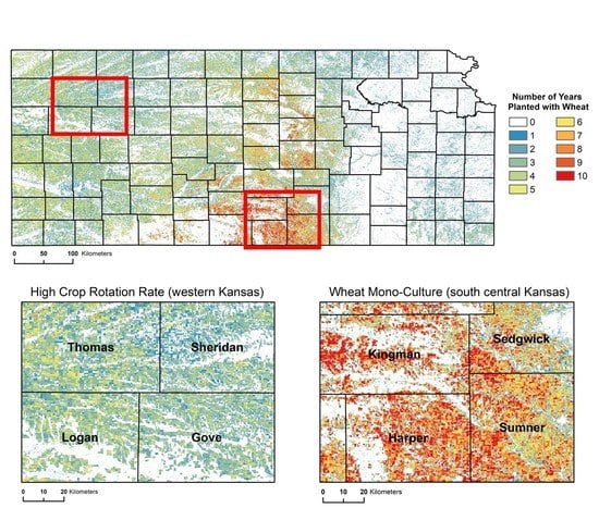
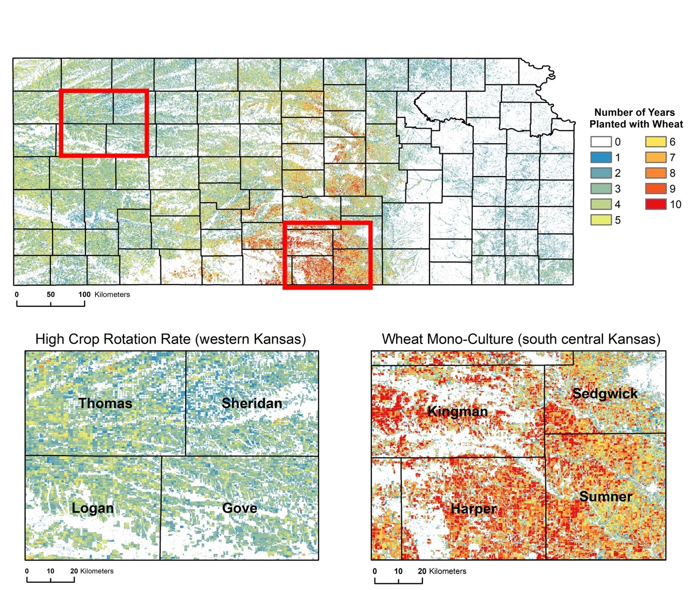
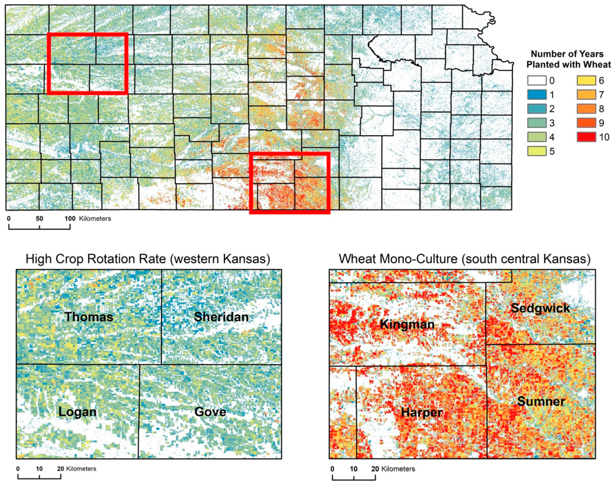
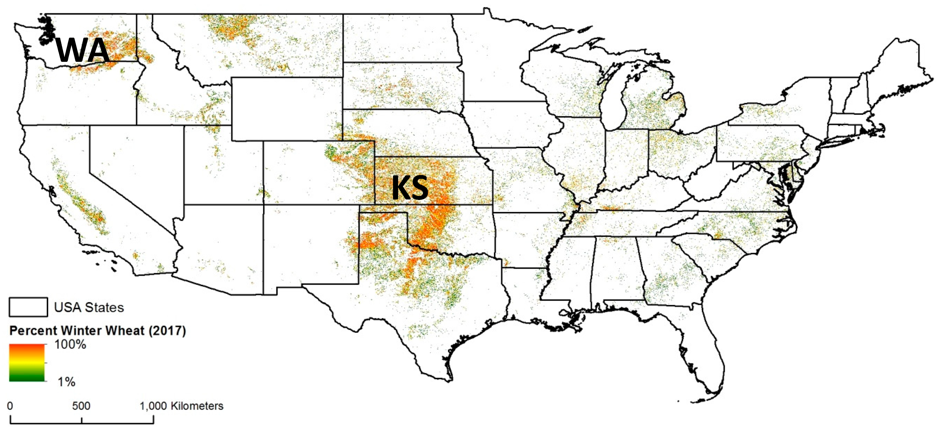
2.1. Study Area

The USA was chosen as the study area for this research, as it is one of the main producers and exporters of wheat globally, and because reliable annual winter wheat classifications are available from the USDA NASS Cropland Data Layer (CDL), which can be used to reliably evaluate our approach.

Amongst field crops in the US, wheat ranks third in terms of planted area behind corn and soy. Wheat is produced in almost every state in the United States and winter wheat varieties dominate US production, representing between 70 and 80% of the total. The main class is Hard Red Winter Wheat, which is grown primarily in the Great Plains, with Kansas being the largest producing state. A study by Yan and Roy on field sizes in the USA [42] found that approximately 85% of wheat fields are smaller than 1 km² and that wheat fields are generally larger than the other crop types for sizes equivalent to between 0.5 × 0.5 mile (0.646 km²) and 0.5 × 1 mile (1.295 km²), which are both common US field sizes.

Due to the widespread practice of crop rotations in many parts of the country, the location of planted wheat fields alternates from one year to the next within the majority of counties. Figure 1 shows an example of crop rotation practices in the particular case of Kansas. Though it should be noted that the total planted area remains relatively constant (Figure 2). According to the USDA NASS statistics, the standard deviation of wheat planted area in the US between 2008 and 2017 was 10% [43].

This study relied on two types of available data: (i) Crop type maps from the USDA NASS Cropland Data Layer (CDL) for eight years, 2008 through 2017, and (ii) NASA MODIS 250 m daily NDVI [44,45]. These datasets are summarized below.

2.2. The USDA NASS Cropland Data Layer (CDL)

The CDL is a crop-specific, rasterized, geo-referenced land-cover map produced by NASS [32,46,47]. NASS is the agency responsible for administering the USDA’s U.S. program, collecting and publishing agricultural statistics at the national, state, and county levels. The CDL is produced annually for the whole United States since 2008 (previous years are also available but just cover the main agricultural states) and is released to the public domain after the growing season and release of official county crop estimates. The CDL layers used in this study were produced by NASS using moderate resolution (30–56 m) imagery from the Indian Advanced Wide Field Sensor (AWiFS), Landsat 5, Landsat 7, the NASS June Agricultural Survey (JAS), and Farm Service Agency (FSA) Common Land Unit for ground truth and training data. The major crop types, including winter wheat, within the CDL generally have a classification accuracy “ranging from mid-80% to mid-90%” [48]. In this study, CDL winter wheat binary masks for 2008 through 2017 were extracted and aggregated to a range of increasingly coarser spatial resolutions in order to investigate the relationship between crop rotation and spatial scale, and the feasibility of using spatially aggregated crop masks to forecast yields.

2.3. Vegetation Index Time Series Data

Vegetation indices (VI) such as NDVI have long been recognized for their value for monitoring vegetation changes as inputs to crop yield and production forecasting models, as well as for tracking crop growth and development [8,25,49,50,51,52,53]. In particular, it has been shown that yield-forecasting models are significantly improved when crop masks are used in conjunction with the VI data, as the crop masks isolate the signal of the crop under investigation [14,54]. In this study, the CDL-derived binary winter wheat masks were scaled up to a range of coarser spatial resolutions as percent wheat masks and used to extract NDVI time-series for winter wheat pixels. These time series were used to estimate winter wheat yields using the GLAM Wheat model, refs. [29,30] to evaluate the utility of coarsening resolution for yield forecasting using a single season wheat mask.

Crops grow and develop rapidly during the growing season. Winter wheat is generally planted in autumn and crop emergence and stand establishment typically occurs in late autumn prior to winter. During winter, vegetative growth slows or ceases and the crop’s resistance to cold weather is increased. In the spring, winter wheat resumes rapid vegetative growth followed by reproductive development and reaches maturity in early to mid-summer. As such, frequent observations are critical for effectively monitoring the crop’s rapid development and state, which currently is only achieved by coarse spatial resolution sensors such as MODIS.

Daily surface reflectance at 250 m resolution from MODIS Collection 6 product (M{O,Y}D09GQ) time-series [44] were obtained for the 2008 through 2017 growing seasons. The surface reflectance product is produced by NASA MODIS Advanced Processing System (MODAPS) [55]. Based on the VJB method [56,57], we derived the nadir Bidirectional reflectance distribution function (BRDF)-corrected surface reflectance, which was used to compute the NDVI using the Red (MODIS band 1, 620 nm–670 nm) and near infrared (MODIS band 2, 841 nm–876 nm) bands [58]:

$$\mathrm{NDVI}=\left(\mathrm{NIR}‒\mathrm{RED}\right)/\left(\mathrm{NIR}+\mathrm{RED}\right).$$

(1)

We used daily surface reflectance observations (M{O,Y}D09GQ) with BRDF corrections rather than the standard MODIS 250 m NDVI product (M{O,Y}D13Q1) for two reasons. Primarily, the MODIS NDVI product is only available as a 16-day or monthly composite while the surface reflectance product corrected for BRDF effects provides daily NDVI at a 250 m resolution. The latter therefore improves the likelihood of capturing the maximum NDVI value. Secondly, the MODIS NDVI product is not BRDF corrected; rather, it is based on a series of criteria that selects the cleanest (i.e., least cloud and aerosol contamination) pixel in the compositing window with the best viewing and illumination geometries. The BRDF correction method normalizes the effects of viewing and illumination geometries, providing a more consistent and comparable value between dates.

3. Methods

This study was carried out in four main steps: (1) spatial aggregation of the 2008–2017 winter wheat masks to increasingly coarser spatial resolution percent-wheat masks; (2) analysis of inter-annual percent wheat variability over eight years at a series of spatial resolutions; (3) extraction of winter wheat-specific NDVI temporal profiles; (4) yield estimation under two scenarios for crop mask availability.

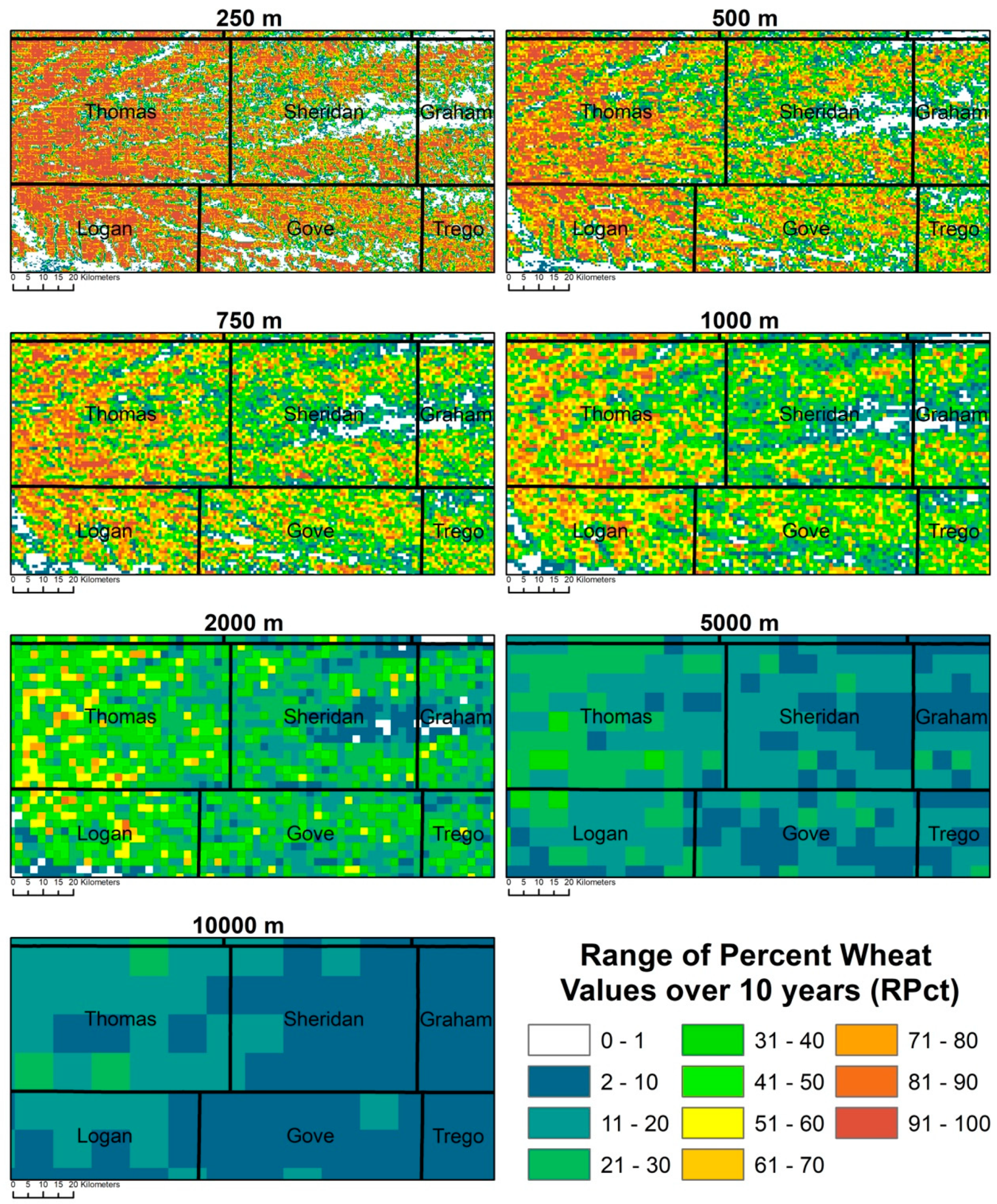
3.1. Spatial Aggregation of Winter Wheat Masks

The US CDLs (2008–2017) were used to create eight binary winter wheat masks at the CDL’s native spatial resolution. The native spatial resolution of the CDL for 2008 and 2009 was limited to 56 m due to the use of AWiFS imagery as input. Subsequent versions of the CDL are available at 30m spatial resolution. At the native resolution wheat pixels were assumed to be pure pixels and therefore assigned a value of 100% and non-wheat pixels were set to 0%. Figure 3 shows an example of the 2017 growing season winter wheat mask at 250 m spatial resolution. These masks were then re-projected to match the MODIS NDVI data sinusoidal projection.

Each of the eight annual winter wheat masks was scaled up to a series of seven, increasingly coarser resolution percent wheat masks for a total of 70 masks, where pixel values represent the proportion of wheat within each pixel. This translates into seven masks for each year between 2008 and 2017 at the following spatial resolutions: 250 m, 500 m, 750 m, 1 km, 2 km, 5 km, and 10 km. At each resolution, the per-pixel wheat percent was calculated by averaging the value of the original resolution binary masks (wheat—100, not wheat—0) within the coarser resolution pixel (Equation (2)). This approach is similar to the spatial aggregation approach commonly described in the literature [59,60,61].

For pixel x at coarse resolution r:

$$Pct{W}_{x,r}=\frac{nCDLWheat}{N}\times 100$$

(2)

where $Pct{W}_{x,r}$ is the scaled-up percent-wheat value for a given pixel x, at coarse resolution r; N is the number of 56 m pixels within pixel x; nCDLWheat is the number of wheat pixels derived from the CDL winter wheat mask within pixel x.

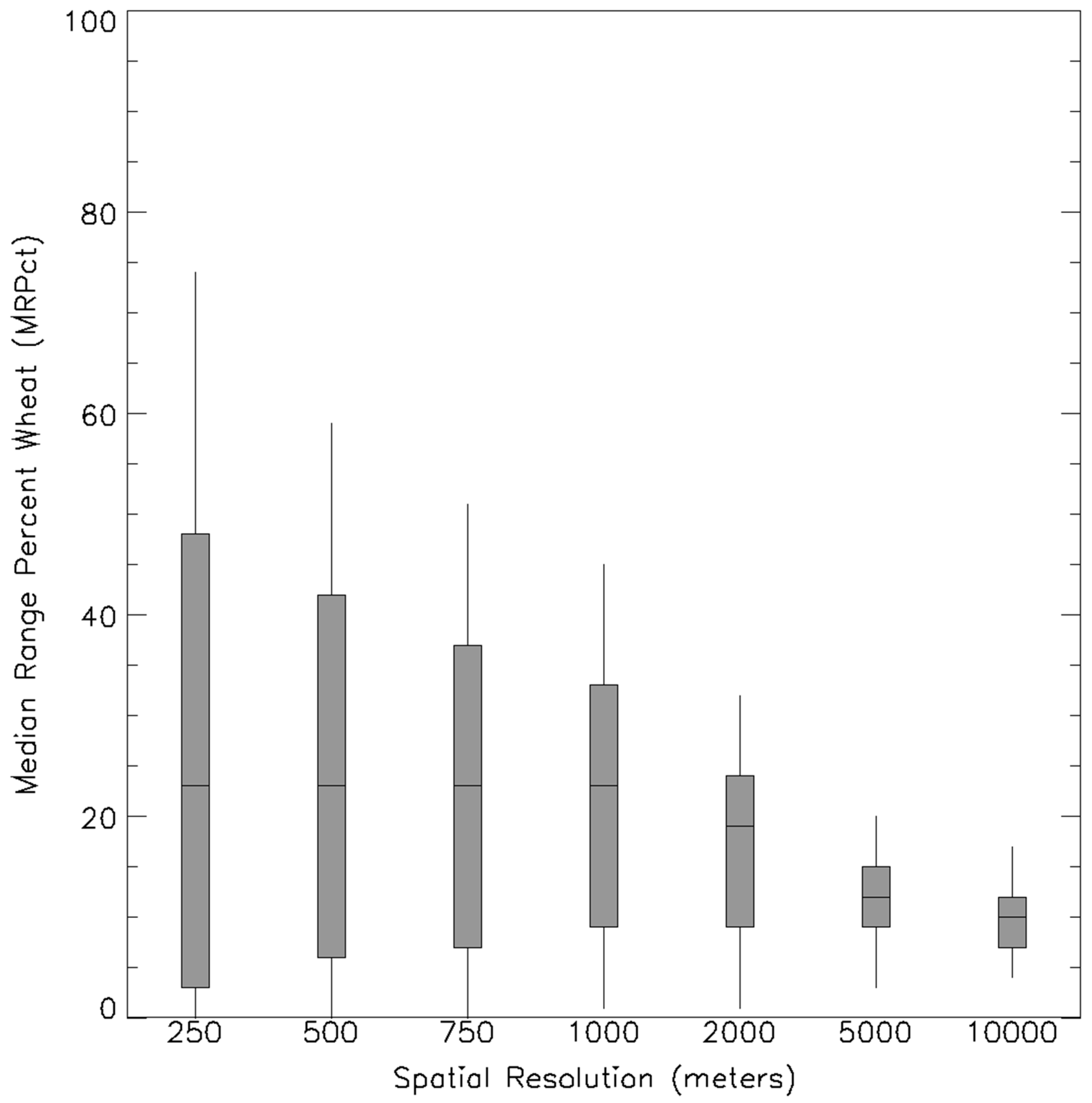
3.2. Analysis of Inter-Annual Percent Wheat Variability

At the basis of the developed approach is the assumption that, at a certain spatial resolution, the percent of wheat within a given pixel remains stable from one year to the next (within a limited number of recent years) despite the practice of crop rotations. Implied is that the overall planted area within the region of interest is relatively constant over the specified time frame. In the case of the US, the winter wheat planted area varied by 10% between 2008 and 2017. Maselli et al. [62] made a similar assumption in a study on wheat production estimation in Tuscany, where they assumed wheat covers a constant fraction of winter crop pixels in all provinces and years used in the study. To assess this assumption in the US and determine the spatial resolution at which the per-pixel wheat purity remains constant over a period of 10 growing seasons, the range of the percent wheat values (RPct) for every pixel (x) at all 7 resolutions (r) was computed (Equation (3)).

$$RPct{W}_{x,r}=Max\left(Pct{W}_{x,r}\right)-Min\left(Pct{W}_{x,r}\right)$$

(3)

where $Max(Pct{W}_{x,r})\mathrm{and}Min(Pct{W}_{x,r})$ are respectively the maximum and the minimum percent wheat value for pixel x at resolution r over 10 years.

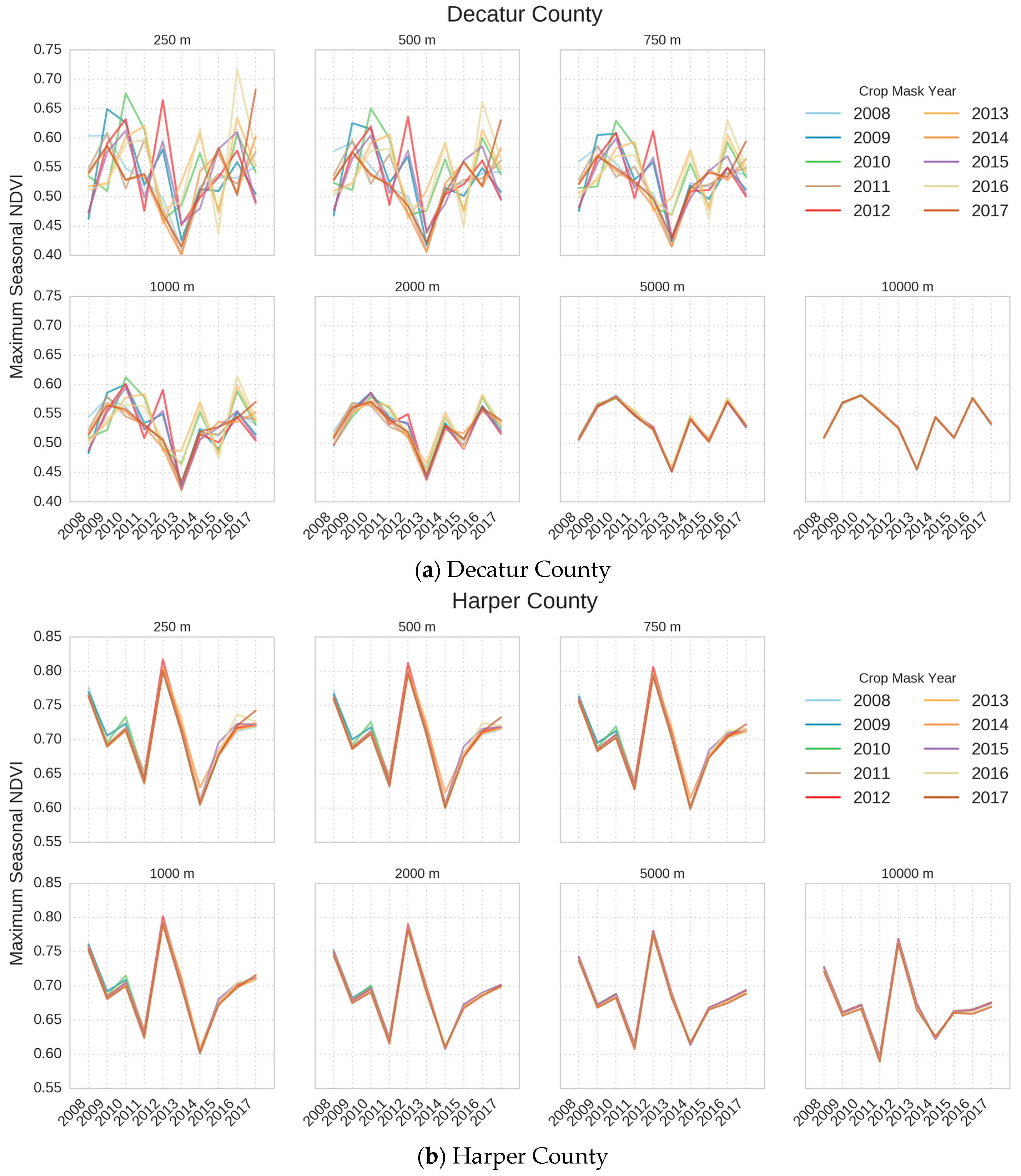
3.3. Winter Wheat-Specific NDVI Time Series

The next step was to evaluate the effect of using a single season percent winter wheat mask for extracting NDVI temporal profiles over multiple years (2008–2017) for the range of spatial resolutions. Following [29], the average NDVI of the 5% purest pixels (VI_wheat) was adjusted for background noise by subtracting the 5% minimum mean NDVI signal through the time series (VI_background) to create a time series for each county (Equation (4)).

$$\begin{array}{c}ANDVI\left(day,county\right)\\ =NDV{I}_{wheat}\left(day,county\right)\\ -{\displaystyle {\displaystyle \sum }_{year=2008}^{2017}}NDV{I}_{background}\left(year,county\right).\end{array}$$

(4)

In order to select the optimal level of spatial aggregation for yield forecasting in the US (accounting for the dampened signal effect as the resolution was coarsened), the GLAM wheat yield model (fully described in [29,30] was run under 2 scenarios of winter wheat mask availability for the full range of pixel spatial resolutions using the extracted MA_NDVI and percent wheat mask as inputs. The wheat mask availability scenarios are described further in Section 3.5.

3.4. GLAM Wheat Yield Model

The GLAM Wheat model, fully described in [29] and [30] is an empirical, generalized regression model based on the assumption that the yield is positively and linearly correlated to the seasonal maximum ANDVI (ANDVI_peak,year) at the county level and to the purity of the wheat signal. The ANDVI_peak,year is estimated averaging the 1% maximum ANDVI values for each year and county. Following [29], the average of the percent wheat values of the purest 5% winter wheat pixels for each county (Mcpt) is used to derive the percent wheat dependent slopes using Equation (5).

$$S_{Mpct}=9.61+\left(-0.05Mpct\right).$$

(5)

We then applied this slope uniformly to the entire US to obtain winter wheat yields in tons/ha for each county by multiplying the ANDVI_peak,year value by the corresponding slope derived (Equation (6)).

$$ForecastYield=ANDV{I}_{peak,year}{S}_{Mpct.}$$

(6)

In this way, the seasonal maximum ANDVI is weighted by the maximum purity that can be observed in each county. The forecast production was finally obtained by multiplying the yield forecast by the official county area harvested statistics.

$$TotalForecastProduction={\displaystyle \sum }_{AU}ForecastYield\times AreaHarvested.$$

(7)

The model was developed in the state of Kansas (USA) and then tested over Ukraine. Franch et al. [30] enhanced the Becker-Reshef et al. [29] model in order to get an improvement on the timeliness of the production forecast by including the information of the accumulated Growing Degree Days (GDD). The model was applied satisfactorily to MODIS and NCEP/NCAR data over the US, Ukraine, and China, and was proven to be applicable to other sensors i.e., VIIRS [63] and Landsat [35]. Most recently, the yield model was applied to AVHRR historical data from 1982 to 2017, over the U.S. [31]. In all these cases, it was able to estimate winter wheat yields within 10% of official statistics, up to two and a half months prior to harvest. The enhanced winter wheat yield model [29,30] is used in this study to estimate yield in this study.

3.5. Yield Estimation under Two Crop Mask Availability Cases

Ideally, detailed and annually updated winter wheat maps would be available during the growing season at an adequate spatial resolution to extract NDVI time series profiles of the target crop. At this time, in-season crop-specific masks are rarely available for the majority of agricultural regions [26,64]. However, a single or a series of crop type maps are often available or can be more easily generated for the previous season, after the growing season is complete.

This study therefore sought to assess the feasibility of using a previous season’s spatially aggregated mask for yield forecasting and to assess the tradeoff between the “optimal” situation where season-specific winter wheat masks are available during the growing season (Case 1—control case) and the most likely situation where only a single mask from the previous season is available (Case 2).

To accomplish this task, the GLAM wheat yield model was run for the two cases at all spatial resolutions. Case 1 was treated as the “control” case representing “optimal” data availability. As such, Case 2 results were assessed relative to the control case. The estimated yields were also assessed against the official NASS reported yields and the root mean square error (RMSE Equation (8)) and corresponding percent error were computed for each case and at each spatial resolution. At the time of this study the NASS winter wheat masks for the whole US were available for 2008 through 2017 so Case 1 was evaluated on these years.

$$RMSE=\sqrt{\frac{{{\displaystyle \sum }}_{i=1}^n{\left(Yiel{d}_f-Yiel{d}_o\right)}^2}{n}}$$

(8)

where n is number of years, Yield_f is the forecast yield, and Yield_O is the observed yield.

In Case 2 (which represents instances when only the previous’ season winter wheat mask is available), the previous season’s mask was used to extract the NDVI signal. In other words, the 2008 mask was used to extract the 2009 growing season NDVI signal and so on. As for Case 1, the RMSE was computed for all Case 2 model runs.

4. Results

4.1. Analysis of Inter-Annual Percent Wheat Variability

A total of 70 percent-wheat masks were created, 7 masks for each year between 2008 and 2017 at the following spatial resolutions: 250 m, 750 m, 500 m, 1 km, 2 km, 5 km, and 10 km. These masks were then used to assess the variability of the per pixel percent wheat at each spatial resolution.

Figure 4 presents a series of images focusing on Western Kansas depicting the RPctW values over 10 years in an area with high crop rotation rates. At finer resolutions (i.e., 250 m), RPctW values were close to 100, indicating that in some years no winter wheat was planted in that location and in other years the pixel was purely winter wheat (Figure 4 shown in red-orange). As pixel size was increased, the variability of percent wheat within a given pixel decreased and stabilized.

To quantify and characterize this percent-wheat “stabilization” effect over the entire country, the median RPctW (MRPct) was computed for all considered counties (Equation (9)) at each of the spatial resolutions and is presented in Figure 5. These results indicate that the percent wheat inter-annual variability drops below 10% after data are aggregated to 5 km for the majority of counties in the US.

$$MRPc{t}_{c,r}=Median\left(RPct{W}_{x,r}\right)|x\in c$$

(9)

where $MRPc{t}_{c,r}$ is the Median Range Percent Wheat for county c at resolution r.

4.2. Winter Wheat-Specific NDVI Time Series

Figure 6a,b shows the results of extracting winter wheat-specific NDVI time series for two contrasting types of counties. Figure 6a for Decatur County, Kansas, where crop rotation is common, and Figure 6b for Harper County, Kansas, where winter wheat monoculture is widespread. Each time-series graph depicts the MA_NDVI signal from 2008 to 2017 extracted using the 10 annual crop masks produced in this step, at all spatial resolutions. In the case of Decatur County, it is evident that a single, season-specific crop mask cannot be used to extract the MA_NDVI at the higher resolutions due to the effect of crop rotations. However, as the resolution is coarsened the extracted signal from each of the crop masks converges, indicating that at coarser resolutions a single mask can be used over multiple years to extract a consistent signal. On the other hand, in Harper County almost all the masks, even at the finer resolutions, can be used to extract a consistent signal since winter wheat fields are not heavily rotated between years.

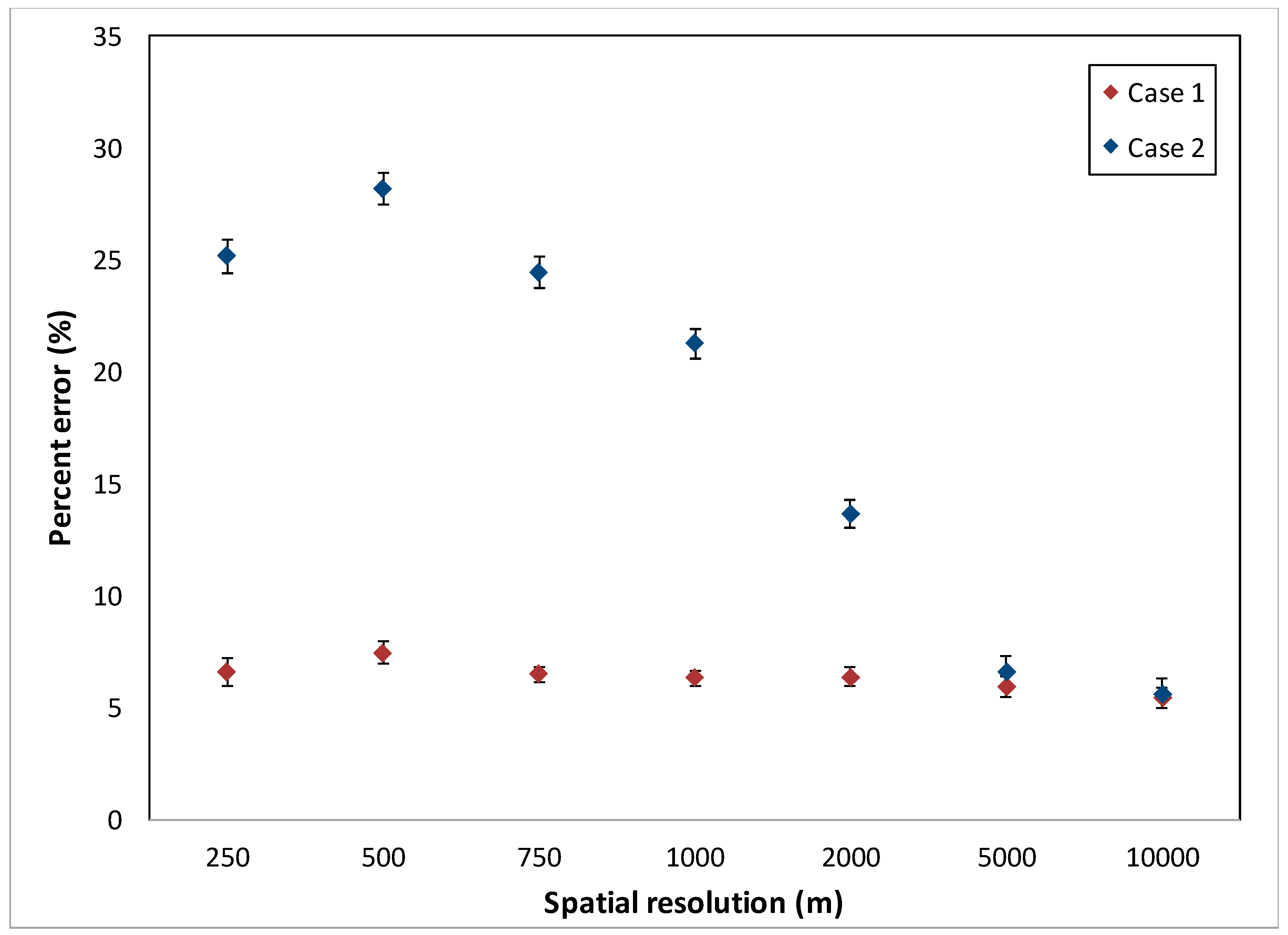
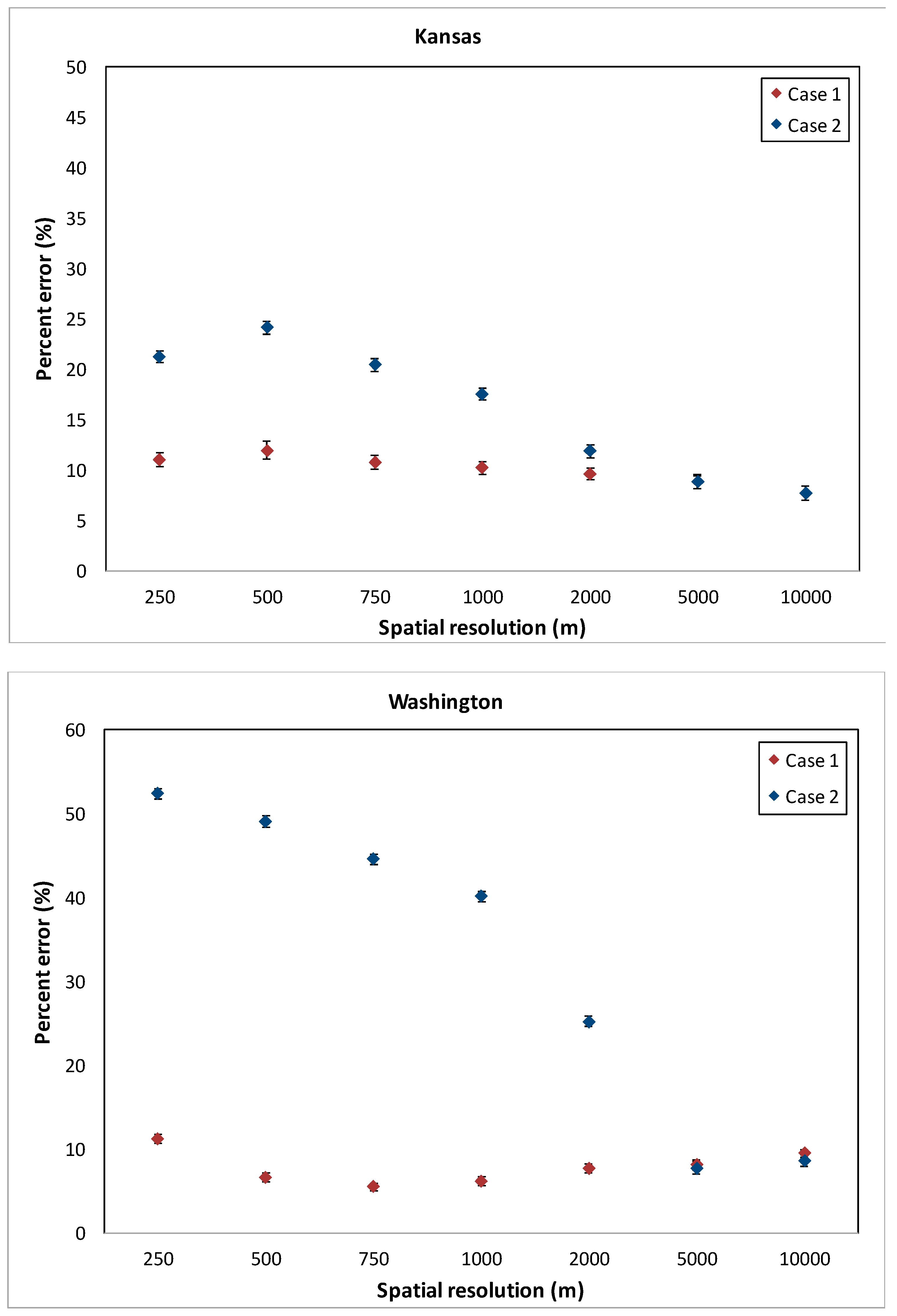
4.3. Yield Estimation under Two Crop Mask Availability Cases

The regression-based winter wheat yield model was run for the cases described. The results for Cases 1 and 2 for the US are presented in Figure 7. Case 1 (red in Figure 7), as expected, had the overall lowest errors (5–6%) with a stable model error across all resolutions given the statistical significance of the results represented by the error bars shown in Figure 7. Case 2 performed poorly relative to Case 1 at the finer resolutions due to the effect of crop rotations, though performed remarkably well as the spatial resolution was coarsened. The error was highest (25–30%) at the finest resolutions, and rapidly declined with coarser spatial resolution with errors equivalent to Case 1 at the 5 and 10 km resolutions.

Figure 8 shows an example of the percent error evolution analogously to Figure 7 but for two contrasting states Kansas and Washington. Kansas shows a lower difference between Case 1 and Case 2 while Washington state shows a larger difference between both cases that can increase up to 50% for the finest spatial resolutions. The reason for such difference in Washington (compared to Kansas) can be explained by the higher overall rate of crop rotation in this state. In both cases, the results provide the same conclusion that the national level plot, with errors from Case 1 and Case 2 equivalent at coarser spatial resolutions.

These results are quite promising as they indicate that, in the absence of a timely seasonal crop-type mask, a single percent wheat mask, derived from a recent season’s crop-type mask, can be used in combination with coarse resolution NDVI to forecast yields prior to harvest. The tradeoff of using a single mask in terms of percent error relative to the Case 1 minimum error (5.4–5.9%) is 0.2–0.7% in Case 2.

5. Discussion and Conclusions

Crop yield forecasting is hampered due to limited availability of detailed crop type masks prior to the end of the growing season. The objective of this study was to develop and evaluate a practical approach to winter wheat yield forecasting that utilizes readily accessible data to forecast yields at sub-national and national scales with minimized tradeoff in accuracy in cases where availability of crop type masks are limited.

To this end, an approach utilizing a single static crop-type mask derived for a preceding season/s, with freely available coarse resolution NDVI time series was evaluated in the US. The approach is based on spatially aggregating moderate resolution (30–56 m) winter wheat masks, to a spatial resolution at which the per-pixel percent wheat remains constant between years enabling extracting a coherent crop-specific NDVI signal from pixels covered with varying proportions of winter wheat. These data were used to run a yield model that utilizes winter wheat percent and maximum seasonal NDVI to forecast yields.

This study found that the best yield estimates were attained when moderate resolution winter wheat masks were available for every season analyzed. However, the tradeoff between using a coarse-resolution, static mask derived from a single preceding season was surprisingly low (0.2–0.7% for 10 and 5 km resolutions, respectively) when compared to the (more optimal) mask representing the current growing season. These results from the US suggest that, in the absence of within-season, detailed crop-specific masks, yield can be forecast at the national level with a small tradeoff in accuracy, using readily available coarse resolution data and a preceding season’s percent wheat mask.

It should be noted that the model provides errors lower than 6% for most spatial resolutions and using in-season crop masks. However, the accuracy of the model decreases for high spatial resolutions, reaching maximum error at 500 m. This is likely due to several factors including the accuracy of the crop masks, artifacts of 250 m gridding such as pixel growth, shift, and distortion (i.e., it has been shown that at the 250 m resolution there can be up to a 0.5 pixel shift [64,65,66,67]). In addition, the simple aggregation approach implemented in this study does not account for the MODIS spatial response, whereby off-nadir sensor acquisitions, i.e., those at increasingly higher view angles, will have a ground sample size greater than acquisitions at the nadir viewing angle (the so-called “bow tie effect”). As pointed out by Duveiller et al. [68], this can impact the percent winter wheat characterization in the aggregated crop type masks. Thus, this topic should be further explored.

While one would assume that, for agricultural remote sensing, it is best to work at the finest spatial resolution so that individual fields can be resolved, this study provides a counter-intuitive result. The results suggest that coarse spatial resolution data with high temporal frequency, combined with lower temporal resolution moderate spatial resolution data, can offer a viable alternative in the absence of finer spatial data and up-to-date crop-specific masks, with a small tradeoff in accuracy in this case. The noise in the crop signal introduced by year-to-year variability due to crop rotations is reduced by monitoring crops at a coarser resolution. This is in keeping with results presented by Markham and Townshend [69], Malingreau and Belward [70], Nelson et al. [61], and more recently Leroux et al. [71], albeit at finer spatial resolutions and for different land cover types.

This study presents a viable and efficient method for isolating a coherent, crop-specific signal over multiple growing seasons using a static, fine resolution crop mask aggregated to a coarse resolution. A fundamental condition for this approach is that there are no major shifts in planted area between years due to such pressures as biofuel demand or market incentives. Nevertheless, according to USDA national level statistics, this condition seems to hold true, at least at the national level, for many of the main wheat exporting countries where the variation in planted area over the past 10 years is below 10% [72]. In the case of the US, where 10 annual national winter wheat masks were available from the USDA NASS, the analysis suggests that over a period of at least 10 years this assumption holds true and that per-pixel percent wheat variability in the US stabilized (below 10%) at approximately 5 km pixel resolution.

The main advantage of the results presented for crop monitoring and specifically for yield forecasting models that rely on remotely sensed inputs is that a single, coarse resolution percent wheat mask is sufficient to extract a consistent winter wheat temporal profile over multiple years. Therefore, a single mask from a previous year would likely suffice. Second, this method helps to mitigate the challenge of generating a timely and accurate crop type mask prior to the end of the growing season in order to forecast yields.

We highlight that the focus of this approach is for forecasting yield over large regions (i.e., at the state or national levels) rather than for precision agriculture purposes or for seasonal crop area estimates. The approach of scaling up a representative seasonal crop-specific mask or a temporally aggregated mask as a percent crop mask is primarily advantageous in regions where crop rotations are common practice. In regions where crop monocultures are prevalent, a single year, moderate resolution crop mask would be as effective. As a coarse resolution crop type mask results in mixed pixels with various crop percentages, a yield model using this approach must explicitly account for the crop percentage as demonstrated in [8] or in Rasmussen et al. [73] as a way of isolating the crop-specific signal. Furthermore, this study only explored such an approach for winter wheat, which has the advantage of greening up prior to summer and spring crops, so further research is needed in order to assess its applicability to other major crop types.

The recent advances in the readily available moderate resolution (20–30 m) data every 3–5 days globally (owing to Sentinels and Landsat), alongside the proliferation in high performance computing and cloud systems, and advances in big data analytics will undoubtedly move the agricultural monitoring community forward, including towards the goal of openly available in-season, moderate-resolution crop type masks. The development of operational capabilities for producing such timely crop type masks, is a high priority for the agricultural monitoring community, as highlighted by the G20 GEOGLAM initiative priorities. At the moment, although significant progress has been made in this direction particularly for the major production regions of the world, (i.e., the Sen2Agri project [74]), these capabilities are still mostly in the applied R&D stages. As such, until such masks are reliably available, the proposed solution in this research seems promising in many of the major production regions (as well as food-insecure ones).

Due to the limited number of seasonal wheat masks that were available to carry out the analysis, it is recognized that the results may be inconclusive and that further assessment should therefore be carried out prior to drawing decisive conclusions. Nevertheless, these results are encouraging and could have promising implications for developing practical, operationally viable methods for crop forecasting at national levels using EO in cases where year-to-year variability of crop area is limited.

References

1. Foley, J.A.; Ramankutty, N.; Brauman, K.A.; Cassidy, E.S.; Gerber, J.S.; Johnston, M.; Mueller, N.D.; O’Connell, C.; Ray, D.K.; West, P.C.; et al. Solutions for a cultivated planet. Nature 2011, 478, 337. [Google Scholar] [CrossRef] [PubMed]
2. Zaks, D.P.M.; Kucharik, C.J. Data and monitoring needs for a more ecological agriculture. Environ. Res. Lett. 2011, 6, 014017. [Google Scholar] [CrossRef]
3. FAO. UN FAO Report on The State of Food Insecurity in the World 2011; UN FAO: Rome, Italy, 2011. [Google Scholar]
4. G20-Agriculture-Ministers. Ministerial Declaration: Action Plan on Food Price Volatility and Agriculture, Meeting of G20 Agriculture Ministers; G20-Agriculture-Ministers: Paris, France, 2011. [Google Scholar]
5. G20-Agricultural-Ministers. G20 Agriculture Ministers’ Declaration 2017: Towards Food and Water Security: Fostering Sustainability, Advancing Innovation; G20-Agriculture-Ministers: Paris, France, 2017. [Google Scholar]
6. Delince, J. Recent Practices and Advances for AMIS Crop Yield Forecasting at Farm/Parcel Level: A Review; FAO: Rome, Italy, 2017. [Google Scholar]
7. Johnson, D.M. An assessment of pre- and within-season remotely sensed variables for forecasting corn and soybean yields in the United States. Remote Sens. Environ. 2014, 141, 116–128. [Google Scholar] [CrossRef]
8. Tucker, C.J.; Holben, B.N.; Elgin, J.H.; McMurtrey, J.E. Relationships of spectral data to grain yield variation. Photogramm. Eng. Remote Sens. 1980, 46, 657–666. [Google Scholar]
9. Lobell, D.B.; Thau, D.; Seifert, C.; Engle, E.; Little, B. A scalable satellite-based crop yield mapper. Remote Sens. Environ. 2015, 164, 324–333. [Google Scholar] [CrossRef]
10. Fritz, S.; See, L.; Bayas, J.C.L.; Waldner, F.; Jacques, D.; Becker-Reshef, I.; Whitcraft, A.; Baruth, B.; Bonifacio, R.; Crutchfield, J.; et al. A comparison of global agricultural monitoring systems and current gaps. Agric. Syst. 2018. [Google Scholar] [CrossRef]
11. Van der Velde, M.; Nisini, L. Performance of the MARS-crop yield forecasting system for the European Union: Assessing accuracy, in-season, and year-to-year improvements from 1993 to 2015. Agric. Syst. 2018. [Google Scholar] [CrossRef]
12. GEO-Agriculture. GEOGLAM: The G-20 GEO Global Agricultural Monitoring Initiative submitted to the G-20 Agriculture Ministers March 23, 2012; GEO: Geneva, Switzerland, 2012. [Google Scholar]
13. FAO. Final Report of the Extraordinary Joint Intersessional Meeting of The Intergovernmental Group (IGG) On Grains and the Intergovernmental Group on Rice, 24, September, 2010; FAO: Rome, Italy, 2010. [Google Scholar]
14. Kastens, J.H.; Kastens, T.L.; Kastens, D.L.A.; Price, K.P.; Martinko, E.A.; Lee, R.-Y. Image masking for crop yield forecasting using AVHRR NDVI time series imagery. Remote Sens. Environ. 2005, 99, 341–356. [Google Scholar] [CrossRef]
15. Azzari, G.; Jain, M.; Lobell, D.B. Towards fine resolution global maps of crop yields: Testing multiple methods and satellites in three countries. Remote Sens. Environ. 2017. [Google Scholar] [CrossRef]
16. Atzberger, C. Advances in Remote Sensing of Agriculture: Context Description, Existing Operational Monitoring Systems and Major Information Needs. Remote Sens. 2013, 5, 949–981. [Google Scholar] [CrossRef] [Green Version]
17. Rasmussen, M.S. Operational yield forecast using AVHRR NDVI data: Reduction of environmental and inter-annual variability. Int. J. Remote Sens. 1997, 18, 1059–1077. [Google Scholar] [CrossRef]
18. Genovese, G.; Vignolles, C.; Negre, T.; Passera, G. A methodology for a combined use of normalised difference vegetation index and CORINE land cover data for crop yield monitoring and forecasting. A case study on Spain. Agronomie 2001, 21, 91–111. [Google Scholar] [CrossRef]
19. Kogan, F.; Guo, W.; Yang, W.; Shannon, H. Space-based vegetation health for wheat yield modeling and prediction in Australia. J. Appl. Remote Sens. 2018, 12, 026002. [Google Scholar]
20. Maselli, F.; Romanelli, S.; Bottai, L.; Maracchi, G. Processing of GAC NDVI data for yield forecasting in the Sahelian region. Int. J. Remote Sens. 2000, 21, 3509–3523. [Google Scholar] [CrossRef]
21. Mkhabela, M.S.; Bullock, P.; Raj, S.; Wang, S.; Yang, Y. Crop yield forecasting on the Canadian Prairies using MODIS NDVI data. Agric. For. Meteorol. 2011, 151, 385–393. [Google Scholar] [CrossRef]
22. López-Lozano, R.; Duveiller, G.; Seguini, L.; Meroni, M.; García-Condado, S.; Hooker, J.; Leo, O.; Baruth, B. Towards regional grain yield forecasting with 1km-resolution EO biophysical products: Strengths and limitations at pan-European level. Agric. For. Meteorol. 2015, 206, 12–32. [Google Scholar] [CrossRef] [Green Version]
23. Kowalik, W.; Dabrowska-Zielinska, K.; Meroni, M.; Raczka, T.U.; de Wit, A. Yield estimation using SPOT-VEGETATION products: A case study of wheat in European countries. Int. J. Appl. Earth Obs. 2014, 32, 228–239. [Google Scholar] [CrossRef]
24. Rojas, O. Operational maize yield model development and validation based on remote sensing and agro-meteorological data in Kenya. Int. J. Remote Sens. 2007, 28, 3775–3793. [Google Scholar] [CrossRef]
25. Funk, C.; Budde, M.E. Phenologically-tuned MODIS NDVI-based production anomaly estimates for Zimbabwe. Remote Sens. Environ. 2009, 113, 115–125. [Google Scholar] [CrossRef]
26. Bolton, D.K.; Friedl, M.A. Forecasting crop yield using remotely sensed vegetation indices and crop phenology metrics. Agric. For. Meteorol. 2013, 173, 74–84. [Google Scholar] [CrossRef]
27. Johnson, D.M. A comprehensive assessment of the correlations between field crop yields and commonly used MODIS products. Int. J. Appl. Earth Obs. 2016, 52, 65–81. [Google Scholar] [CrossRef] [Green Version]
28. Guan, K.; Wu, J.; Kimball, J.S.; Anderson, M.C.; Frolking, S.; Li, B.; Hain, C.R.; Lobell, D.B. The shared and unique values of optical, fluorescence, thermal and microwave satellite data for estimating large-scale crop yields. Remote Sens. Environ. 2017, 199, 333–349. [Google Scholar] [CrossRef]
29. Becker-Reshef, I.; Vermote, E.; Lindeman, M.; Justice, C. A generalized regression-based model for forecasting winter wheat yields in Kansas and Ukraine using MODIS data. Remote Sens. Environ. 2010, 114, 1312–1323. [Google Scholar] [CrossRef]
30. Franch, B.; Vermote, E.; Becker-Reshef, I.; Claverie, M.; Huang, J.; Zhang, J.; Justice, C.; Sobrino, J. Improving the timeliness of winter wheat production forecast in the United States of America, Ukraine and China using MODIS data and NCAR Growing Degree Day information. Remote Sens. Environ. 2015, 161, 131–148. [Google Scholar] [CrossRef]
31. Franch, B.; Vermote, E.; Roger, J.-C.; Murphy, E.; Becker-Reshef, I.; Justice, C.; Claverie, M.; Nagol, J.; Csiszar, I.; Meyer, D.; et al. A 30+ Year AVHRR Land Surface Reflectance Climate Data Record and Its Application to Wheat Yield Monitoring. Remote Sens. 2017, 9, 296. [Google Scholar] [CrossRef]
32. Boryan, C.; Yang, Z.; Mueller, R.; Craig, M. Monitoring US agriculture: The US Department of Agriculture, National Agricultural Statistics Service, Cropland Data Layer Program. Geocarto Int. 2011, 26, 341–358. [Google Scholar] [CrossRef]
33. McNairn, H.; Kross, A.; Lapen, D.; Caves, R.; Shang, J. Early season monitoring of corn and soybeans with TerraSAR-X and RADARSAT-2. Int. J. Appl. Earth Obs. 2014, 28, 252–259. [Google Scholar] [CrossRef]
34. Vaudour, E.; Noirot-Cosson, P.E.; Membrive, O. Early-season mapping of crops and cultural operations using very high spatial resolution Pléiades images. Int. J. Appl. Earth Obs. Geoinf. 2015, 42, 128–141. [Google Scholar] [CrossRef]
35. Skakun, S.; Vermote, E.; Roger, J.-C.; Franch, B. Combination of Landsat-8 and Sentinel-2a for Winter Wheat Yield Assessment at Regional Level; NASA: Washington, DC, USA, 2017.
36. Villa, P.; Stroppiana, D.; Fontanelli, G.; Azar, R.; Brivio, P. In-Season Mapping of Crop Type with Optical and X-Band SAR Data: A Classification Tree Approach Using Synoptic Seasonal Features. Remote Sens. 2015, 7, 12859. [Google Scholar] [CrossRef]
37. Waldner, F.; De Abelleyra, D.; Verón, S.R.; Zhang, M.; Wu, B.; Plotnikov, D.; Bartalev, S.; Lavreniuk, M.; Skakun, S.; Kussul, N.; et al. Towards a set of agrosystem-specific cropland mapping methods to address the global cropland diversity. Int. J. Remote Sens. 2016, 37, 3196–3231. [Google Scholar] [CrossRef] [Green Version]
38. Hao, P.; Zhan, Y.; Wang, L.; Niu, Z.; Shakir, M. Feature Selection of Time Series MODIS Data for Early Crop Classification Using Random Forest: A Case Study in Kansas, USA. Remote Sens. 2015, 7, 5347. [Google Scholar] [CrossRef]
39. Kussul, N.; Lavreniuk, M.; Skakun, S.; Shelestov, A. Deep Learning Classification of Land Cover and Crop Types Using Remote Sensing Data. IEEE Geosci. Remote. Sens. 2017, 14, 778–782. [Google Scholar] [CrossRef]
40. Skakun, S.; Franch, B.; Vermote, E.; Roger, J.-C.; Becker-Reshef, I.; Justice, C.; Kussul, N. Early season large-area winter crop mapping using MODIS NDVI data, growing degree days information and a Gaussian mixture model. Remote Sens. Environ. 2017, 195, 244–258. [Google Scholar] [CrossRef]
41. Wardlow, B.; Egbert, S. Large-area crop mapping using time-series MODIS 250 m NDVI data: An assessment for the U.S. Central Great Plains. Remote Sens. Environ. 2008, 112, 1096–1116. [Google Scholar] [CrossRef]
42. Yan, L.; Roy, D.P. Conterminous United States crop field size quantification from multi-temporal Landsat data. Remote Sens. Environ. 2016, 172, 67–86. [Google Scholar] [CrossRef]
43. NASS. NASS Quick Stats; USDA National Agricultural Statistics Service (NASS): Washington, DC, USA, 2012.
44. Vermote, E.F.; Kotchenova, S. Atmospheric correction for the monitoring of land surfaces. J. Geophys. Res. Atmos. 2008, 113. [Google Scholar] [CrossRef] [Green Version]
45. Vermote, E.; Roger, J.-C.; Ray, J.P. MODIS Surface Reflectance User’s Guide Collection 6; NASA Goddard Space Flight Center: Greenbelt, MD, USA, 2015.
46. Mueller, R.; Boryan, C.; Seffrin, R. Data partnership synergy: The Cropland Data Layer. In Proceedings of the 2009 17th International Conference on Geoinformatics, Fairfax, VA, USA, 12–14 August 2009; pp. 1–6. [Google Scholar]
47. NASS. CropScape-Cropland Data Layer. Available online: http://nassgeodata.gmu.edu/CropScape/ (accessed on 18 September 2018).
48. NASS. CropScape and Cropland Data Layers FAQs. Available online: https://www.nass.usda.gov/Research_and_Science/Cropland/sarsfaqs2.php#Section3_18.0 (accessed on 18 September 2018).
49. Pinter, P.J.; Jackson, R.D.; Idso, S.B.; Reginato, R.J. Multidate spectral reflectances as predictors of yield in water stressed wheat and barley. Int. J. Remote Sens. 1981, 2, 43–48. [Google Scholar] [CrossRef]
50. Hatfield, J.L. Remote sensing estimators of potential and actual crop yield. Remote Sens. Environ. 1983, 13, 301–311. [Google Scholar] [CrossRef]
51. Maselli, F.; Conese, C.; Petkov, L.; Gilabert, M.A. Environmental Monitoring and Crop Forecasting in the Sahel through the Use of Noaa Ndvi Data—A Case-Study—Niger 1986–89. Int. J. Remote Sens. 1993, 14, 3471–3487. [Google Scholar] [CrossRef]
52. Rasmussen, M.S. Assessment of Millet Yields and Production in Northern Burkina-Faso Using Integrated NDVI from the Avhrr. Int. J. Remote Sens. 1992, 13, 3431–3442. [Google Scholar] [CrossRef]
53. Quarmby, N.A.; Milnes, M.; Hindle, T.L.; Silleos, N. The Use of Multitemporal NDVI Measurements from AVHRR Data for Crop Yield Estimation and Prediction. Int. J. Remote Sens. 1993, 14, 199–210. [Google Scholar] [CrossRef]
54. Doraiswamy, P.C.; Hatfield, J.L.; Jackson, T.J.; Akhmedov, B.; Prueger, J.; Stern, A. Crop condition and yield simulations using Landsat and MODIS. Remote Sens. Environ. 2004, 92, 548–559. [Google Scholar] [CrossRef]
55. Masuoka, E.; Roy, D.; Wolfe, R.; Morisette, J.; Sinno, S.; Teague, M.; Saleous, N.; Devadiga, S.; Justice, C.O.; Nickeson, J. MODIS land data products: Generation, quality assurance and validation. In Land Remote Sensing and Global Environmental Change: NASA’s Earth Observing System and the Science of ASTER and MODIS; Ramachandran, B., Justice, C.O., Abrams, M.J., Eds.; Springer: Berlin, Germany, 2011; Volume 11, p. 873. [Google Scholar]
56. Vermote, E.; Justice, C.O.; Breon, F.M. Towards a Generalized Approach for Correction of the BRDF Effect in MODIS Directional Reflectances. IEEE Trans. Geosci. Remote Sens. 2009, 47, 898–908. [Google Scholar] [CrossRef]
57. Franch, B.; Vermote, E.F.; Sobrino, J.A.; Julien, Y. Retrieval of Surface Albedo on a Daily Basis: Application to MODIS Data. IEEE Trans. Geosci. Remote Sens. 2014, 52, 7549–7558. [Google Scholar] [CrossRef]
58. Tucker, C.J. Red and photographic infrared linear combination for monitoring vegetation. Remote Sens. Environ. 1979, 8, 127–150. [Google Scholar] [CrossRef]
59. Woodcock, C.E.; Strahler, A.H. The Factor of Scale in Rmeote Sensing. Remote Sens. Environ. 1987, 21, 311–332. [Google Scholar] [CrossRef]
60. Morisette, J.T.; Nickeson, J.E.; Davis, P.; Wang, Y.J.; Tian, Y.H.; Woodcock, C.E.; Shabanov, N.; Hansen, M.; Cohen, W.B.; Oetter, D.R.; et al. High spatial resolution satellite observations for validation of MODIS land products: IKONOS observations acquired under the NASA Scientific Data Purchase. Remote Sens. Environ. 2003, 88, 100–110. [Google Scholar] [CrossRef] [Green Version]
61. Nelson, M.D.; McRoberts, R.E.; Holden, G.R.; Bauer, M.E. Effects of satellite image spatial aggregation and resolution on estimates of forest land area. Int. J. Remote Sens. 2009, 30, 1913–1940. [Google Scholar] [CrossRef]
62. Maselli, F.; Moriondo, M.; Angeli, L.; Fibbi, L.; Bindi, M. Estimation of wheat production by the integration of MODIS and ground data. Int. J. Remote Sens. 2011, 32, 1105–1123. [Google Scholar] [CrossRef]
63. Justice, C.O.; Vermote, E.; Bandaru, V.; Becker-Reshef, I.; Franch, B.; Sullivan, M. Transitioning from MODIS to S-NPP VIIRS data for Agricultural Monitoring. In Proceedings of the American Geophysical Union, Fall General Assembly, San Francisco, CA, USA, 12–16 December 2016. [Google Scholar]
64. Duveiller, G.; Baret, F.; Defourny, P. Remotely sensed green area index for winter wheat crop monitoring: 10-Year assessment at regional scale over a fragmented landscape. Agric. For. Meteorol. 2012, 166, 156–168. [Google Scholar] [CrossRef]
65. Bréon, F.M.; Vermote, E.; Murphy, E.F.; Franch, B. Measuring the Directional Variations of Land Surface Reflectance From MODIS. IEEE Trans. Geosci. Remote Sens. 2015, 53, 4638–4649. [Google Scholar] [CrossRef]
66. Tan, B.; Woodcock, C.E.; Hu, J.; Zhang, P.; Ozdogan, M.; Huang, D.; Yang, W.; Knyazikhin, Y.; Myneni, R.B. The impact of gridding artifacts on the local spatial properties of MODIS data: Implications for validation, compositing, and band-to-band registration across resolutions. Remote Sens. Environ. 2006, 105, 98–114. [Google Scholar] [CrossRef]
67. Wolfe, R.E.; Roy, D.P.; Vermote, E. MODIS land data storage, gridding, and compositing methodology: Level 2 grid. IEEE Trans. Geosci. Remote Sens. 1998, 36, 1324–1338. [Google Scholar] [CrossRef]
68. Duveiller, G.; Baret, F.; Defourny, P. Crop specific green area index retrieval from MODIS data at regional scale by controlling pixel-target adequacy. Remote Sens. Environ. 2011, 115, 2686–2701. [Google Scholar] [CrossRef]
69. Markham, B.; Townshend, J.R.G. Land cover classification accuracy as a function of sensor spatial resolution. In Proceedings of the 15th International Symposium on Remote Sensing of Environment, Ann Arbor, MI, USA, 11–15 May 1981; pp. 1839–1852. [Google Scholar]
70. Malingreau, J.P.; Belward, A.S. Scale considerations in vegetation monitoring using AVHRR data. Int. J. Remote Sens. 1992, 13, 2289–2307. [Google Scholar] [CrossRef]
71. Leroux, L.; Baron, C.; Zoungrana, B.; Traoré, S.B.; Seen, D.L.; Bégué, A. Crop Monitoring Using Vegetation and Thermal Indices for Yield Estimates: Case Study of a Rainfed Cereal in Semi-Arid West Africa. IEEE J. Stars 2016, 9, 347–362. [Google Scholar] [CrossRef]
72. USDA. Production Supply Distribution Online. 2018; USDA. Available online: http://www.fas.usda.gov/psdonline/ (accessed on 24 September 2018).
73. Rasmussen, M.S. Developing simple, operational, consistent NDVI-vegetation models by applying environmental and climatic information. Part II: Crop yield assessment. Int. J. Remote Sens. 1998, 19, 119–139. [Google Scholar] [CrossRef]
74. Bontemps, S.; Arias, M.; Cara, C.; Dedieu, G.; Guzzonato, E.; Hagolle, O.; Inglada, J.; Matton, N.; Morin, D.; Popescu, R.; et al. Building a data set over 12 globally distributed sites to support the development of agriclutre monitoring applications with sentinel-2. Remote Sens. 2015, 7, 16062–16090. [Google Scholar] [CrossRef]
Figure 1. Crop rotation rates in Kansas over 10 years: 2008–2017. Low rotation rates are in red (i.e., no rotation where 10 out of 10 years were planted with wheat) and high rotation rates are in green-blue. Top panel shows the entire state and the lower panels highlight two contrasting areas. Left panel is an area where crop rotation is widespread, and the right panel is an area with a wheat mono-culture.
Remotesensing 10 01659 g001
Figure 2. Evolution of the US winter wheat harvested area.
Remotesensing 10 01659 g002
Figure 3. USA percent winter wheat mask of the 2017 growing season at 250 m.
Remotesensing 10 01659 g003
Figure 4. Example of RPct values computed from 10 annual winter wheat masks for increasingly coarser resolutions over Western Kansas where crop rotation is common practice. The upper left corner shows a 250 m resolution; the lower left corner shows a 10,000 m resolution. Red indicates high variability in per pixel percent wheat; blue indicates near constant percent wheat across years.
Remotesensing 10 01659 g004
Figure 5. Boxplot of median range percent winter wheat (MRPct) for all counties considered in the US, computed for each spatial resolution using the 2008–2017 wheat masks.
Remotesensing 10 01659 g005
Figure 6. (a,b) Maximum Seasonal NDVI extracted for 2008 through 2017 using eight seasonal winter wheat masks (2008–2017). Line colors are presented according to the year of the wheat mask. Data were extracted at increasingly coarser resolutions. Upper left: 250 m; lower right: 10 km. (a) Data from Decatur County where wheat fields are commonly rotated. (b) Data from Harper County where wheat monoculture is the dominant practice.
Remotesensing 10 01659 g006
Figure 7. Model percent error in the US for each case evaluated. Case 1: season-specific wheat masks are available during the growing season (control case). Case 2: a single detailed crop type mask is available from a previous recent season. The error bars represent the standard deviation of all possible RMSEs leaving one year out from the analysis for the 10 years considered (2008–2017).
Remotesensing 10 01659 g007
Figure 8. Model percent error in Kansas and Washington states for each case evaluated analogously to Figure 7. The error bars represent the standard deviation of all possible RMSEs leaving one year out from the analysis for the 10 years considered (2008–2017).
Remotesensing 10 01659 g008