Airborne Laser Scanning Cartography of On-Site Carbon Stocks as a Basis for the Silviculture of Pinus Halepensis Plantations

Abstract

Forest managers are interested in forest-monitoring strategies using low density Airborne Laser Scanning (ALS). However, little research has used ALS to estimate soil organic carbon (SOC) as a criterion for operational thinning. Our objective was to compare three different thinning intensities in terms of the on-site C stock after 13 years (2004–2017) and to develop models of biomass (Wt, Mg ha⁻¹) and SOC (Mg ha⁻¹) in Pinus halepensis forest, based on low density ALS in southern Spain. ALS was performed for the area and stand metrics were measured within 83 plots. Non-parametric kNN models were developed to estimate W_t and SOC. The overall C stock was significantly higher in plots subjected to heavy or moderate thinning (101.17 Mg ha⁻¹ and 100.94 Mg ha⁻¹, respectively) than in the control plots (91.83 Mg ha⁻¹). The best W_t and SOC models provided R² values of 0.82 (W_t, MSNPP) and 0.82 (SOC-S₁₀, RAW). The study area will be able to stock 134,850 Mg of C under a non-intervention scenario and 157,958 Mg of C under the heavy thinning scenario. High-resolution cartography of the predicted C stock is useful for silvicultural planning and may be used for proper management to increase C sequestration in dry P. halepensis forests.

1. Introduction

Climate change is one of the major environmental concerns [1]. It has been related to the emission of greenhouse gases (GHG) by human activities, of which carbon dioxide (CO₂) represents 40% [2]. The assimilation of atmospheric CO₂ by forest ecosystems though photosynthesis is a key process in net primary production and in the mitigation of climate change. Annually, forest ecosystems present a positive balance of CO₂ exchange with the atmosphere; thus, they are considered as carbon sinks [3,4]

Carbon (C) is stored in forest ecosystems not only in tree biomass but also in litter and forest soils. Indeed, soils are the major terrestrial C pool and sink for atmospheric CO₂ (>71%), of which >50% occurs in the upper horizons [5,6]. Soil C exists in organic and inorganic forms. Soil organic carbon (SOC) is one of the most important soil components affecting plant growth and plant nutrients cycles [6]. Moreover, it can be stored in soils for thousands of years, under adequate conditions. However, SOC storage can be affected by climatic conditions, aboveground biomass, forest management, land-use patterns, human activities and other factors [7].

It has been demonstrated that the management of forests can positively influence C sequestration [8,9,10]. The rate of growth for tree biomass can be increased by active management; therefore, the potential C sequestration rates in managed forests might increase too [11]. Thinning enhances tree growth and the early productivity of forests [12], while soil C might exhibit initial losses with a later recovery once the canopy cover is restored [7]. The rates of C sequestration and storage in forest plantations managed by selective harvesting might, in the long term, exceed those of unmanaged forest plantations [10,11]. However, most of the studies about the influence of thinning on long-term forest C sequestration have been performed in northern latitudes and for mature forest, while there are few studies in semiarid ecosystems or for forest plantations (but see [13,14,15]). This raises the question: what is the role of silviculture in the long-term potential C sequestration in semiarid forest plantations?

In Spain, Aleppo pine (Pinus halepensis Mill.) has been one of the tree species most commonly used in afforestation, accounting for over two million hectares at different elevations (0–1000 m a.s.l.). Its plantations were installed on different soil substrates, leading to diverse forest structures for which one can emphasize their role in soil protection [16]. However, the plantations of P. halepensis in southern Spain represent some of the forests most threatened by climate change in the Mediterranean Basin [17]. Silvicultural practices, such as thinning, are an important management operation and have a major impact on Aleppo pine stand development and conservation, particularly on stand density. Aleppo pine responds well to thinning and this operation stimulates the growth of the remaining trees by decreasing the competition for resources [18,19]. Thinning enhances the photosynthetic capacity of the crown due to an increase in the foliar mass of the remaining trees and in the light reaching the lower parts of the crown [20], though the thinning effect on SOC is still unclear. These forest plantations become homogeneous and high density stands, which require thinning treatments to guarantee the provision of goods and services. Although one to two silvicultural thinning interventions are typically applied during a rotation of P. halepensis stands [21], in many cases few or none have been applied [22]. However, forest managers strongly recommend the use of silvicultural treatments to manipulate stand densities and tree growth, in order to maintain and increase C stocks [22,23] and to encourage sustainable forest management, thereby mitigating climate change effects on Aleppo pine forests (e.g., [24,25,26,27])

Nowadays, with the advances in remote sensing techniques, the field-based inventory has been replaced and/or supplemented by Airborne Laser Scanning (ALS). ALS is a laser-based remote sensing technology that is used extensively for many forestry purposes and it provides data that are highly accurate with regard to predicting forest metrics and reducing inventory costs, when compared to traditional stand-level inventories [28]. As a result, forest attributes metrics—such as basal area, height, tree diameter at breast height, stand density and volume, which describe the state of the stand while assisting directly the thinning decisions [29]—have been estimated using modelling algorithms and ALS data [15,28,30,31,32].

There are numerous modelling algorithms available for the estimation of forest metrics with ALS [33]. Of these, we selected nearest neighbours (kNN) [34]. Nearest neighbours techniques are multivariate, non-parametric methods, which given an unlabelled object finds a group of k most similar objects and uses them to assign a class label to match the class of the majority of the k similar cases in the training neighbourhood [34]. Since the 1990s, kNN techniques have been progressively applied to forest inventory and remotely sensed data when estimating and mapping forest attributes—particularly growing stock volume, biomass and C stock variables, and, to a lesser extent, basal area and tree density [35]. In particular, forest inventory and ALS information together with the kNN technique have been used effectively to calculate aboveground biomass data [34].

Despite the timely and accurate estimates of forest structure obtained using ALS in forest inventories, little research has used this technology to estimate the C stocks of Mediterranean Aleppo pine forests (but see [15]). Thus, the assessment and mapping of heterogeneous stand densities, in relation to thinning management and total C stocks (SOC and biomass) at the stand level are challenging and have been poorly studied. In this study, we used low density ALS (0.5 points m⁻²) data from the Spanish National Plan for Aerial Orthophotography (PNOA), together with kNN techniques, to predict aerial biomass, SOC and on-site C stocks in stands of P. halepensis plantations under different thinning intensities. The specific objectives were: (i) to evaluate the effect of different thinning intensities (moderate and heavy), in comparison to unthinned P. halepensis stands, on the C stocks in biomass and SOC; (ii) to assess the accuracy of the estimation of C stocks based on low density ALS data and a kNN algorithm; and (iii) to quantify C stocks at the forest management unit scale. We worked with data collected in a 57-year-old P. halepensis plantation and ALS data (with low pulse density) acquired in 2014 at the national scale. The results are discussed in the context of the implementation of airborne ALS systems to monitor forest C stocks and emission reduction programs

2. Materials and Methods

2.1. Study Area

The study was conducted in the forested areas of “Los Cuadros” (Murcia region, south-eastern Spain, 38°05′18″N, 1°06′18″W; 1437.2 ha) (Figure S1, Supporting Information). The elevation of the study area ranges from 140 to 280 m a.s.l. and the steepness of the slopes is −15–20%. The parent material is composed of limestone and the representative soils of the study area are haplic calcisols [36] with inclusions of lithic leptosols, very common in the region of Murcia because the soils develop in an arid climate and have low moisture content. Annual rainfall ranges between 250 and 350 mm and the annual average temperature is 18.2 °C, with warm (mean maximum temperature in summer is 26.3 °C) and dry summers (mean precipitation in summer is 8.2 mm; Murcia meteorological station, 38°06′28″N, 01°03′18″W, 104 m a.s.l.). The managed forests are dominated by a pure P. halepensis plantation (57 years-old) established on abandoned agricultural land between 1950 and 1960 with an initial plant density of 1400 tree ha⁻¹. Tree growth is poor, with tree heights ranging from 4 to 12 m and normal diameter (diameter at breast height) from 8 to 30 cm. The understory is composed of Mediterranean evergreen shrubs (Cistus albidus L., Stipa tenacissima L., Anthyllis cytisoides L., Rosmarinus oficinalis L., Pistacea lentiscus L., Rhamnus lycioides L. and Chamaerops humilis L.).

2.2. Field Data

In July 2014, 47 plots were established within the forested areas of “Los Cuadros” (Figure S1, Table S1, Supporting Information). The plots were located randomly, considering representative canopy structural parameters with a variable radius plot sampling. In each plot, the diameter at breast height (1.3 m above ground level –dbh– cm), stand density (N, trees ha⁻¹), basal area (G, m² ha⁻¹) and height (H, m) of all trees greater than or equal to 10 cm (dbh) were measured using a calliper (Haglöf Mantax, Långsele, Sweden) and Vertex III hypsometer (Haglöf, Sweden).

Additionally, thinning treatments were applied between August and November 2004 (for more details, see [17]). A factorial randomized block design was used, considering three thinning intensity treatments, unthinned-control, moderate thinning (M) with removal of 33% of the initial basal area (mean remaining density of 770 trees ha⁻¹ and tree basal area of 6.6 m² ha⁻¹) and heavy thinning (H) with removal of 50% of the initial basal area (mean remaining density of 550 trees ha⁻¹ and tree basal area of 4.5 m² ha⁻¹) and three replicate blocks (

Table 1. Silvicultural characteristics, biomass and soil organic carbon stocks (Mg ha⁻¹) of Pinus halepensis plantations according to the thinning intensity (C, Control or unthinned plots; T30, light thinning, 30% basal area removed; T50, heavy thinning, 50% of basal area removed) at Los Cuadros (Murcia, Spain). Variables and abbreviations: stem density (D, trees ha⁻¹); height (H, m); diameter at breast height (dbh, cm); basal area (G, m² ha⁻¹), Biomass C stock (W_t, Mg C ha⁻¹) and Soil Organic Carbon stock (SOC_depth –S, Mg C ha⁻¹). Values are means ± SE. Different letters indicate significant post-hoc differences between thinning treatments at alpha = 0.05 based on a one-way ANOVA.

	Control	Moderate Thinning	Heavy Thinning
Silvicultural Characteristics (Post Thinning)
D (trees ha−1)	1400	770	550
H (m)	6.9 (0.2)	6.7 (0.162)	6.8 (0.2)
dbh (cm)	14.1 (0.7)	14.1 (0.5)	14.9 (0.4)
G (m2 ha−1)	24.6 (2.6)	12.8 (0.8)	10.0 (0.6)
Biomass C stock (Mg C ha−1)
Stems	16.4 (2.1)a	8.05 (0.5)b	5.21 (0.4)c
Medium branches	3.71 (0.4)a	1.78 (0.8)b	1.20 (0.7)b
Small branches and foliate	10.12 (1.1a	5.06 (0.2)b	3.38 (0.2)c
Roots	11.42 (1.1)a	6.43 (0.3)b	4.14 (0.2)c
Biomass stock (Wt)	41.65 (4.8)a	21.32 (0.8)b	13.93 (1.4)b
Soil Organic Carbon stock (Mg C ha−1)
0–10 cm	11.50 (0.81)c	19.07 (0.9)b	30.92 (2.6)a
10–20 cm	14.03 (1.1)b	21.82 (1.8)a	26.51 (3.4)a
20–30 cm	13.83 (1.4)b	20.17 (2.0)a	16.09 (1.9)ab
30–40 cm	10.82 (0.8)b	18.56 (2.8)a	13.72 (1.7)b
SOC40-S	50.18 (1.7)c	79.62 (1.9)b	87.24 (3.1)a
Wt + SOC10-S	53.15 (3.1)a	40.39 (1.5)b	44.85 (3.0)b
Wt + SOC40-S	91.83 (4.0)b	100.94 (1.4)a	101.17 (2.6)a

). All blocks (60 × 120 m each) were located on moderately steep (less than 20%) slopes. Each replicate block was divided into two adjacent plots of 60 × 60 m each and each plot was assigned one of the two thinning treatments: heavy or moderate. In July 2017, three new plots, located close by, were set up to incorporate the control treatment, considering identical pre-thinning canopy structural parameters and site conditions (slopes <20% and NW exposure), because it was not included in the original thinning design [17], giving a total experimental area of 3.24 ha. The thinning treatments were applied for the primary purpose of removing overtopped, small-sized, dying, or suppressed trees to promote stand species diversification [17], with additional consideration given to uniform spacing. Thinning residues, such as slashes and stumps, were removed from the treatment plots, although some of the slash was left on-site. On these plots, structural plots (N = 36, radius = 10 m) were also established and dbh, N, G and H were measured in July 2017 (Table 1). Total aboveground biomass was estimated using the allometric models included, as the sum of the fractions calculated using biomass (kg) Equations (1)–(4) derived for P. halepensis on a nationwide basis [37]:

$$\mathrm{Ws}=0.0139\times {\mathrm{d}}^2\times \mathrm{h};\mathrm{RMSE}:21.43$$

(1)

W_b7 = [3.926 × (d − 27.5)] × Z; RMSE: 14.75
If d ≤ 27.5 cm then Z = 0; If d > 27.5 cm then Z = 1;

(2)

W_b2−7 = 4.257 × 0.00506 × d² × h − 0.0722d × h; RMSE: 7.54

(3)

W_b2+n = 6.197 × 0.00932 × d² × h − 0.0686 d × h; RMSE: 13.79

(4)

Ws: Biomass weight of the stem fraction. W_b7: Biomass weight of the thick branch fraction with a diameter greater than 7 cm; W_b2–7: Biomass weight of the medium branch fraction with a diameter between 2 and 7 cm; W_b2+n: Biomass weight of the thin branch fraction with a diameter smaller than 2 cm, with needles (all in kg); d = dbh (cm); h = tree height (m). Overall biomass (W_t) was expressed in Mg ha⁻¹ (Table 1). A standard coefficient of 0.5 [38] was used to obtain the biomass C content.

2.3. Soil Sampling and Analysis

In July 2017, 36 soil point survey samples (4 per plot and 12 per treatment) were taken systematically in the thinning and control plots, considering similar canopy structural parameters in areas with slopes <20%. The samples were taken using an 8-cm-diameter steel auger and were transported to the laboratory undisturbed. In the laboratory, all the soil soundings were cut into four sections: 0–10, 10–20, 20–30 and 30–40 cm, in the first part of the mineral soil. All the soil samples were air-dried, then coarse particles were removed with a sieve (mesh size 2 mm); the resultant fine earth fraction was ground to pass through a 0.5-mm mesh and stored for SOC determination. In the sieving process, all particulate organic matter (rootlets, leaves, seeds and other plant material) was manually extracted. The gravel (>2 mm) was weighed and stored separately. For each soil sample, three replicates of each measurement were performed in the laboratory.

The organic carbon content of the fine fraction was determined through wet oxidation by the Walkley and Black method [39]. The bulk density (BD) in the soil layers was estimated as follows [40] (g cm⁻³):

$$\mathrm{BD}=\frac{100}{\frac{\%\mathrm{OM}}{0.244}+\frac{100-\%\mathrm{OM}}{1.64}}$$

(5)

where SOM (soil organic matter) was obtained with the expression %OM = %SOC × 1.724. We used a typical value of 1.64 for mineral bulk density [41].

The soil organic C stock (SOC-S, Mg ha⁻¹) was calculated for each layer and expressed in Mg ha⁻¹ according to [42]:

SOC-S = SOC × BD × D

(6)

where SOC% = soil organic carbon (%), BD = bulk density of the soil (g cm⁻³) and D = thickness of the analysed layer (cm). The overall soil organic carbon stock (SOC₄₀-S) in the first 40 cm from the soil surface was calculated by adding together the values obtained for each layer.

2.4. ALS Data and Processing

Figure 1 includes a flow diagram of the complete methodological process used in this study.

Low density ALS (0.5 points m⁻²) data were provided by the PNOA (http://www. ign.es/PNOA/vuelo_ALS.html, [43]); these systematically cover the entire Spanish national territory. The ALS survey was conducted using an airborne Leica ALS60 discrete return sensor. A total of 1.55 Gb large of ALS data were provided and captured in 2009 and were delivered in three 2 km × 2 km tiles (ranging from 86 Mb to 136 Mb) of raw data points in a ASPRS laser LAS binary file, format v. 1.1, containing x- and y-coordinates (UTM Zone 30 ETRS 1989), ellipsoidal elevation Z, with up to four returns measured per pulse and intensity values from a 1064-nm wavelength laser [15]. The resulting ALS point density of the test areas was the ALS and the flight parameters, used to achieve first-return densities that averaged 1-point m² with a vertical accuracy higher than 0.20 m, were a scan frequency of 45 Hz and a FOV of 50°.

For all structural and soil plots (N = 83), overlapped with each soil sample in the thinning and control plots (N = 36), a synthetic ALS plot cloud was obtained. The time delay between the ALS data acquisition and the field data collection (i.e., the 5–8 years) was not considered a significant source of error, as the pine forest under study did not change considerably during that period (mean annual increment= 1.71 ± 0.025 mm year⁻¹). A sub-meter global satellite receiver (Leica Zeno 20 GIS, Leica Geosystems, Switzerland) was used to survey plot centres and soil samples. We computed ALS metrics to support a kNN regression model, based on previous research by [30]. The metrics involved in the equation of the C stock model were obtained using the “GridMetrics” and “CSV2Grid” commands implemented in FUSION LDV 3.30 [44]. In summary, the ALS point clouds were first filtered to generate a Digital Elevation Model (DEM) (cell size 0.5 m) and ALS metrics were computed for each ALS plot after normalizing the data by subtraction of the DEM. In this study, a total of 43 metrics was extracted from ALS pulses and used as regressors in the statistical analyses. The ALS-based height metrics obtained in each plot were: minimum, maximum, mean, median, standard deviation, variance, coefficient of variation, interquartile distance, skewness, kurtosis, ADD (average absolute deviation), L-Moments (1–4) and percentile values (P₅ to P₉₅ in five-unit intervals and P₉₉) [45]. For further details of the procedure used to obtain such ALS metrics, see the steps described in Reference [46]. To obtain a complete explanation of the FUSION tools, see [44]. The summary of the ALS metrics with their corresponding descriptions is shown in Table S1, Supporting Information.

2.5. Data Analysis and k-NN Predictions

Prior to statistical analysis, we examined all variables for normality using the Kolmogorov-Smirnov test (with Lilliefors correction). Homoscedasticity was analysed by the Levene’s test of variance (p > 0.05). When the variables were not normal, the data were subjected to a Box-Cox transformation. The results in the tables are shown as means with their standard errors for the untransformed variables. The biomass and SOC stocks were analysed with one-way analysis of variance (ANOVA). When a global difference among the thinning treatments was detected, means were separated by Scheffe’s multiple range test for unequal sample sizes, for normal and homoscedastic variables [47]. Differences among treatments were considered significant at a significance level of p = 0.05.

Possible relationships among ALS metrics and G, N, W_t-S (N = 83) and SOC-S (N = 36) were determined using the k-Nearest Neighbour (kNN) machine-learning algorithm [48]. For the C stock, five models were evaluated, considering W_t-S, SOC-S at a depth of 0–10 cm (SOC-S₁₀) and 0–40 cm (SOC-S₄₀), W_t-S + SOC-S₁₀ and W_t-S + SOC-S₄₀. This method does not require statistical assumptions about the nature of the data; for instance, normality or homoscedasticity [48]. Explanatory variables were selected, firstly using variance inflation factor (VIF) analysis to check multicollinearity [33] and secondly choosing the variable or combination of variables which minimized the generalized root mean square distance when variables were added or deleted one at a time [49]. Thus, once the best predictor variables had been selected, we tested nine variations of the distance metric, Euclidean distance (EUC), Euclidian distance without standardization (RAW), Malahanobis distance (MAL), independent component analysis (ICA), similar neighbour (MSN), weighted neighbour more similar (MSN2), similar neighbour with canonical correlation analysis via projection pursuit (MSNPP), nearest neighbour gradient (GNN) and random forest (RF) [50]. We estimated the accuracy of the Knn predictions by three validation procedures; internal validation, external validations and cross-validation. Internal validation was assessed using the entire dataset to develop and validate model prediction, that is, model predictions were run and evaluated with the entire dataset. External validation was performer by data partitioning according to the 60/40 ratio, 60% of the data was used for training and 40% of the data for evaluation purpose. Finally, leave one out cross-validation was used to select the best model which was evaluated by mean of leave one out cross validation [49]. The election of the k value is a compromise between bias and precision in the estimation [51]. However, when variance in the imputations is similar to variance in the observations a single nearest neighbour k is appropriate [52], therefore we used k = 3 in our analysis. We compared the bias and RMSE values of each method:

$$RMSE=\sqrt{\frac{1}{n}{\displaystyle \sum _{i=1}^n}({\widehat{y}}_i}-y_i{)}^2$$

(7)

$$BIAS=\frac{{\sum }_{i=1}^n({\widehat{y}}_i-y_i)}{n}$$

(8)

Finally, we compared the performances of all methods by graphing observed versus predicted values and calculating a Pearson correlation coefficient.

We performed all analyses using the R software, version 3.4.0. [53] The yaImpute R package [49] was used to calculate variable selection and regression with kNN, the lm and glm libraries were used for ANOVAs and the usdm package was used to perform collinearity analysis [54].

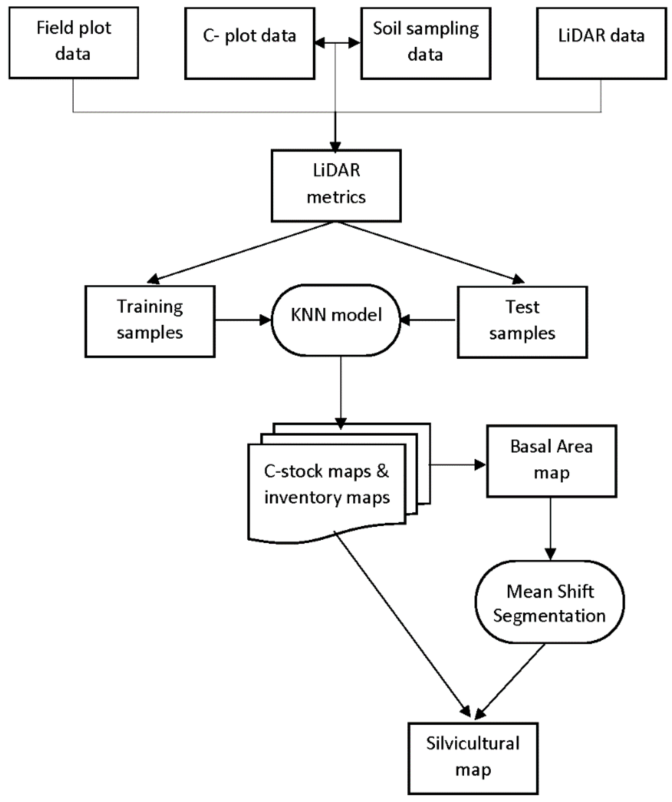
2.6. Cartography of C Stocks

Finally, a C stock map of the P. halepensis cover in the study area was generated. First, stands were segmented using the mean shift segmentation method, with Orfeo ToolBox software (OTB) for QGIS’s [55]. Basal area per hectare (G) was the silvicultural variable used to identify and group data into single stands. Mean shift segmentation is based on non-parametric Kernel density estimation (KDE). The algorithm works by looking for local maxima in the feature-space, by moving a Parzen window towards them incrementally [56]. Once a local maximum has been detected, clustering of data points is accomplished [57,58]. The algorithm needs three parameters to be set: (1) the spatial radius to define the neighbourhood, (2) the range radius to define the interval in the spectral space and (3) the minimum size of the regions to keep after clustering. For this study, the first two parameters were ranged to cover all segmentation possibilities, while the value of the minimum size of the region was kept constant at 10,000 m², which was considered as the minimum size for silvicultural operations. The best stand segmentation was selected using the validation method in Reference [59].

Then, five C stock maps—W_t-S, SOC-S₁₀, SOC-S₄₀, W_t-S + SOC-S₁₀ and W_t-S + SOC-S₄₀—were generated at the stand scale by applying the best kNN algorithm (highest R² and lowest RMSE) based on the Murcia vegetation map (http://www.murcianatural.carm.es/alfresco/montes/index.html). The map of vegetation of Murcia has been used to define the limits of the study area provided by the Forest Service of Murcia and segmentation has been used to define the internal stands of the forest area. The pixel size selected to compute the ALS-derived metrics and to map the C stock was 18 m × 18 m, representing an area of 324 m², similar to the field plot dimensions (314 m²).

Finally, a silvicultural map based on the C stock and stand density was generated at the stand scale, to allow estimation of the net balance between the non-intervention and heavy thinning scenarios with regard to CO₂ absorption and economic balance, considering the current price on the C market (18.88 € (Mg CO₂)⁻¹, http://www.worldbank.org/en/programs/pricing-carbon).

3. Results

3.1. C Stock in Biomass and SOC under Different Thinning Intensities

The biomass C stocks for all fractions and thinning treatments are presented in Table 1. The C stock in the aboveground biomass was much higher in the control treatment (41.65 Mg ha⁻¹, F = 17.86, p < 0.001) than in the thinning treatments (21.32 Mg ha⁻¹ and 13.93 Mg ha⁻¹, for M and H, respectively). The C stock distribution in biomass was similar among all treatments, where the combination of branches and stems corresponded to ~70% of the total biomass, over the thinning time (13 years). The C stock in the aboveground biomass was significantly higher for all fractions in the control than in the M and H treatments (p < 0.001), although it was higher in M than in H. The C stock in the belowground biomass decreased with the intensity of the thinning regime, with a mean value of 11.42 Mg C ha⁻¹ for the control and a mean reduction of 43.6% for M and 63.7% for H (F = 22.54, p < 0.001, Table 1).

Mineral soils comprised the largest C pool stock, with significant differences in SOC-S between thinning treatments (Table 1). The SOC₄₀-S values of the composite soil samples (0–40 cm) were 50.18 Mg ha⁻¹ (control), 79.62 Mg ha⁻¹ (M) and 87.24 Mg ha⁻¹ (H), with the first horizon (0–10 cm) contributing 22.9% (11.5 Mg ha⁻¹), 23.9% (19.0 Mg ha⁻¹) and 35.4% (30.9 Mg ha⁻¹), respectively, of the total SOC measured (Table 1). The SOC-S was significantly higher (p < 0.001) under treatment H for the 0–20 depth, while the values were highest for treatment M in the rest of the layers (Table 1). The value of W_t + SOC₁₀-S was higher for control plots (53.15 Mg ha⁻¹) than for the M (40.39 Mg ha⁻¹) and H (44.85 Mg ha⁻¹) thinned plots, with significant differences (F = 4.61, p < 0.005, Table 1). However, the overall C stock (W_t + SOC₄₀-S) was significantly higher in the H and M thinned plots (101.17 Mg ha⁻¹ and 100.94 Mg ha⁻¹, respectively) than in the control plots (91.83 Mg ha⁻¹, F = 7.80, p < 0.001, Table 1). The SOC₄₀-S accounted for 54.6% of the total on-site C stock in the control, 78.8% in treatment M and 86.2% in treatment H. There was a 9.9% increase in the on-site C stock for treatment M and a 10.1% increase in the case of treatment H, in comparison with the unthinned plots.

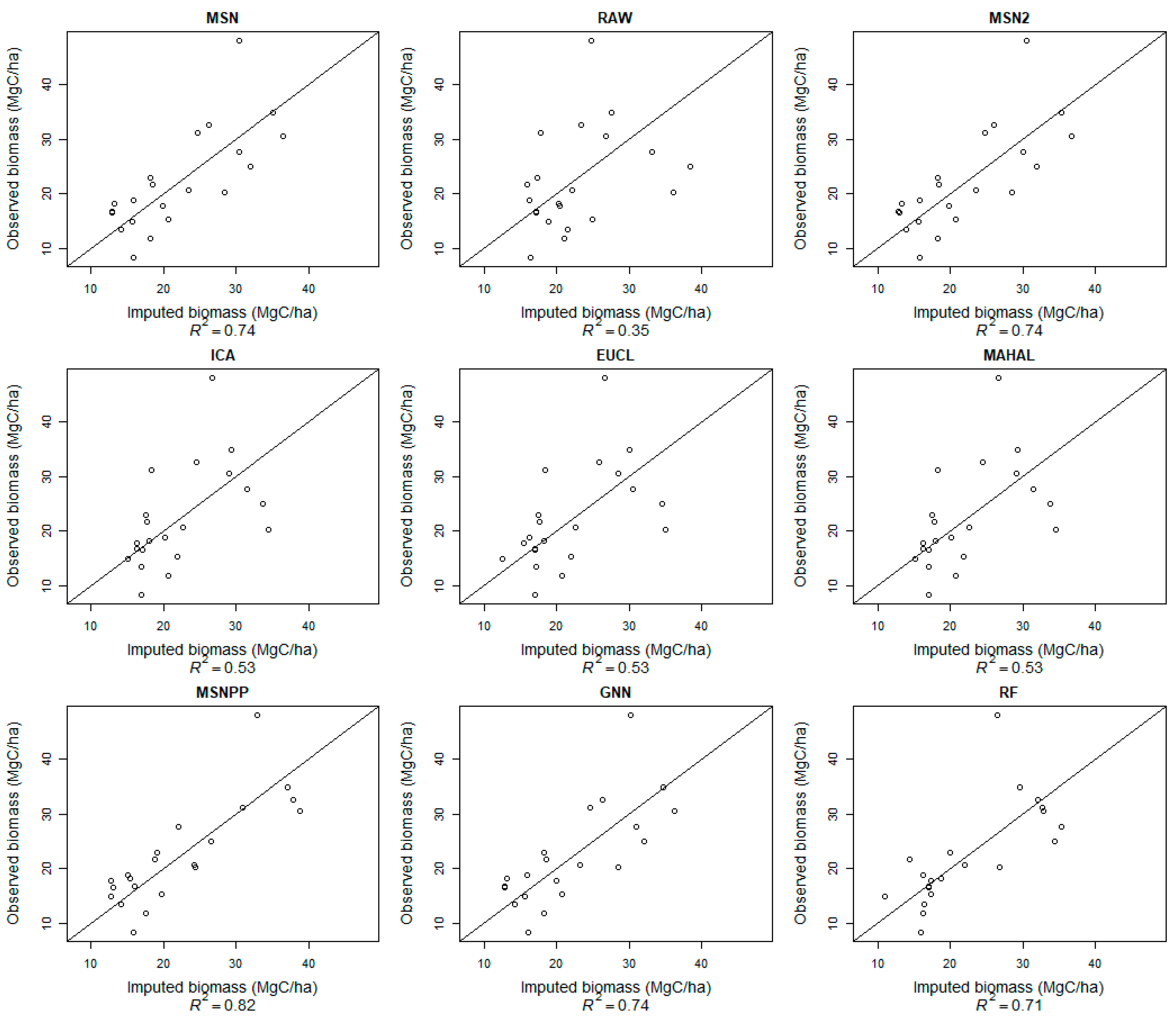
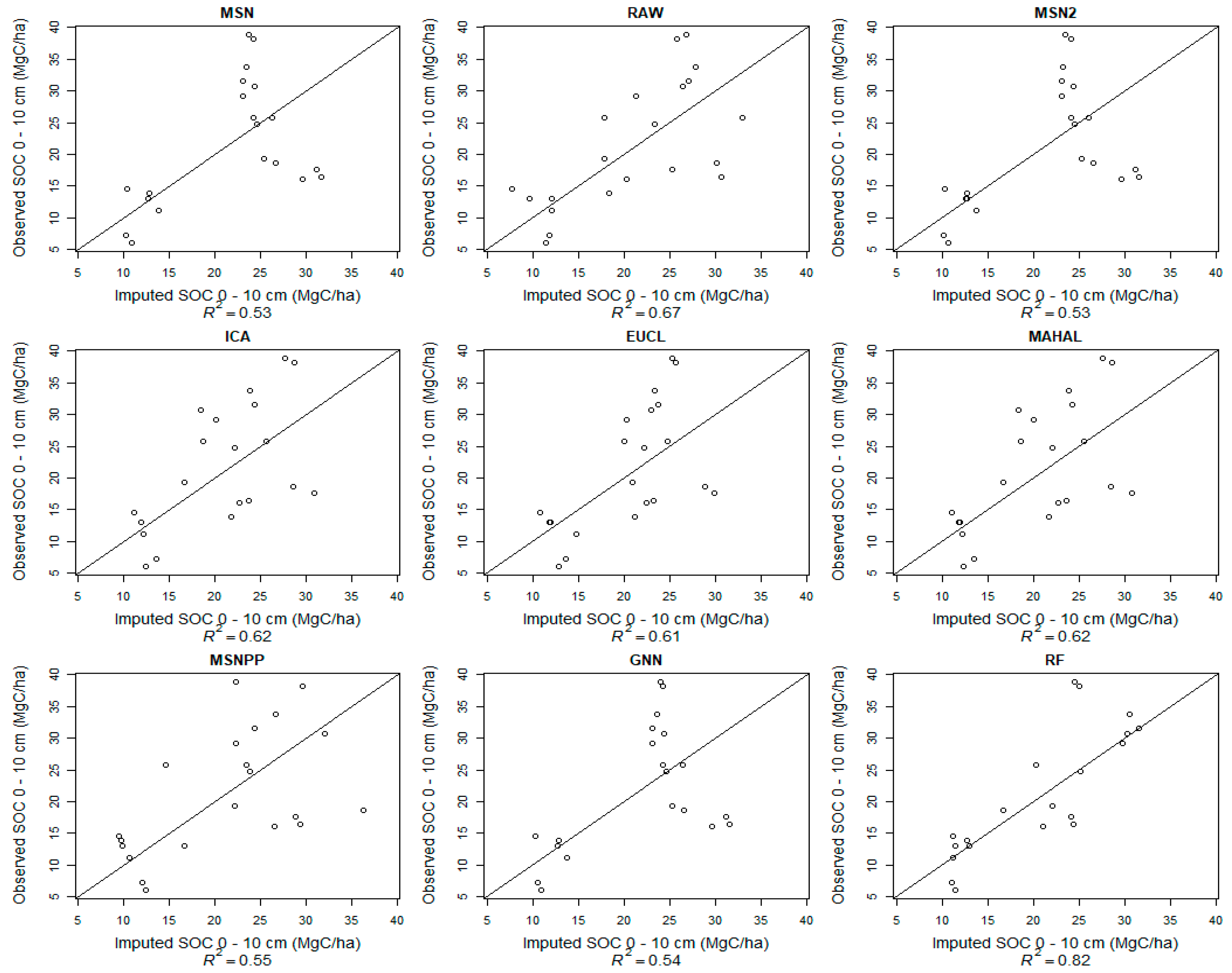
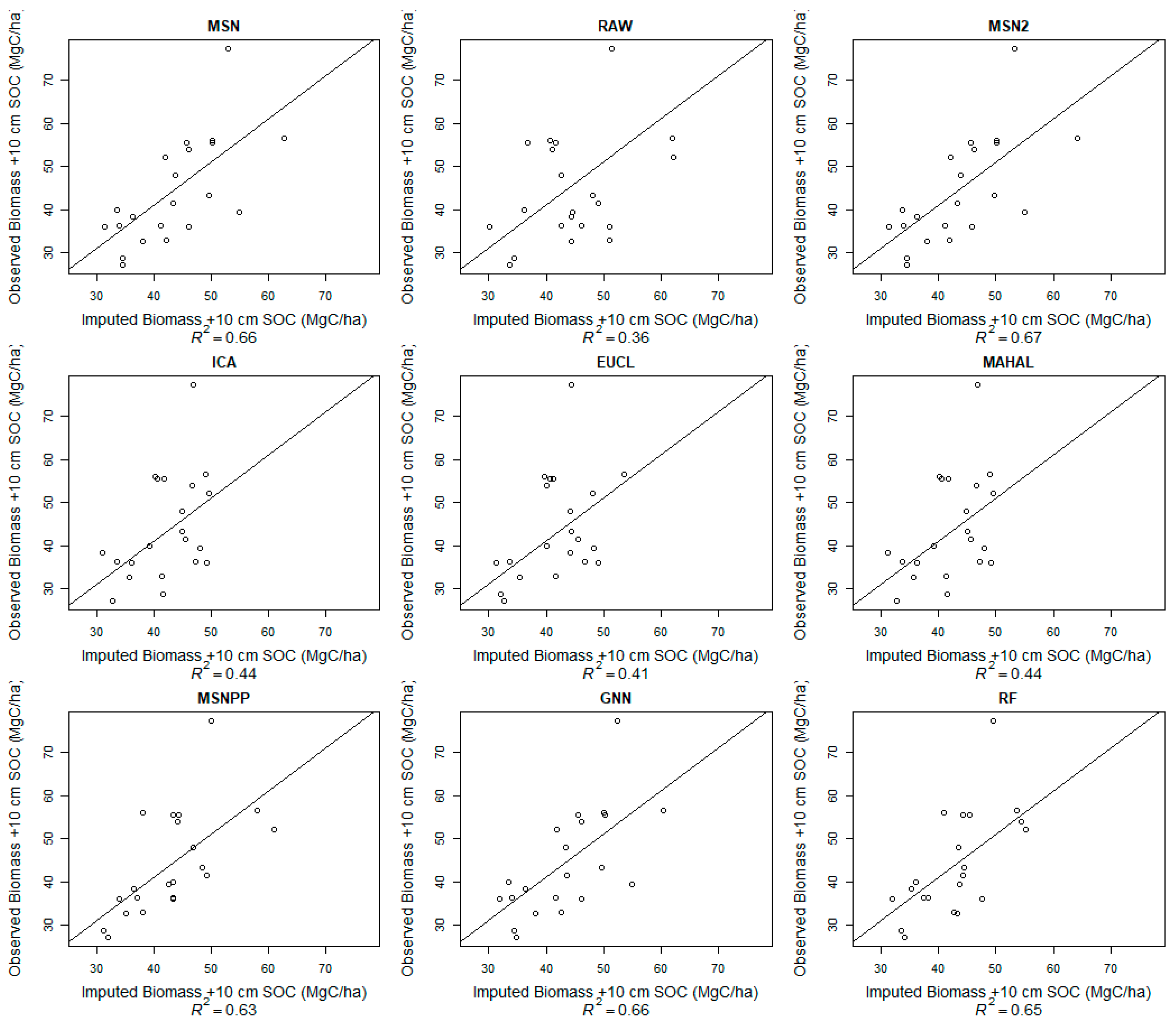
3.2. kNN Models for C Stocks

Following the independent variable data selection, all models used the height variable (H_P₆₀, H_P₉₉) and returns above mean (Percentage first returns above, all returns above mean) (

Table 2. Variable importance classification of kNN models between biomass and SOC C stocks and LiDAR metrics of Pinus halepensis plantations at Los Cuadros (Murcia, Spain). In bold are shown the variables selected to run the models.

	Variable	Rank	Mean	SD
A	Height percentile P60	1	1.330	0.108
B	Height percentile P99	2	1.319	0.101
C	Percentage first returns above mode	3	1.315	0.100
D	All returns above mean	4	1.306	0.084
E	Height percentile P50	5	1.282	0.095
F	Height percentile P75	6	1.279	0.083

, Figure S2; Table S2 Supplementary Material). The predictor variables had a moderate to high correlation with the forest dasometric variables (N, H and G), which suggests that LiDAR metrics are a good representation of the forest metrics.

We computed the scatter plots for correlations contrasting the observed versus the estimated values for all C stocks predictions, to select the best estimation based on the kNN method (Figure 2, Figure 3, Figure 4, Figures S3 and S4, Supplementary Material;

Table 3. Root-mean-square error (RMSE) and bias of bivariate relationships between LiDAR metrics and biomass C stock (Mg C ha⁻¹) and Soil Organic Carbon stock (SOC_depth –S, Mg C ha⁻¹) models of Pinus halepensis plantations at Los Cuadros (Murcia, Spain).

Error	MSN	MSN2	EUCL	RAW	MALAH	ICA	MSNPP	GNN	RF
Biomass Stock
RMSE	8.05	8.05	9.44	11.62	8.89	8.89	8.03	8.05	9.17
% RMSE	35.44	35.44	41.54	51.14	39.15	39.15	35.34	35.44	40.36
BIAS	0.92	0.92	−2.06	0.68	−1.58	−1.58	0.68	0.92	−0.41
%BIAS	4.04	4.05	−9.07	3.02	−6.94	−6.94	3.01	4.05	−1.79
SOC10 stock (0–10 cm soil layer)
RMSE	4.87	4.87	4.97	4.66	4.91	4.91	4.40	4.87	4.35
% RMSE	21.33	21.33	21.79	20.40	21.50	21.50	19.28	21.33	19.07
BIAS	−0.01	−0.01	−0.05	−0.83	−0.03	−0.03	−0.55	−0.01	−1.19
%BIAS	−0.04	−0.04	−0.21	−3.65	−0.13	−0.13	−2.40	−0.04	−5.22
Biomass + SOC10 stock (0–10 cm soil layer)
RMSE	9.36	15.95	9.36	12.84	14.44	12.84	10.93	9.36	9.85
% RMSE	21.31	36.28	21.31	29.20	32.83	29.20	24.87	21.31	22.41
BIAS	1.01	3.89	1.01	−0.87	−3.01	−0.87	0.91	1.01	−3.21
%BIAS	2.29	8.86	2.29	−1.97	−6.84	−1.98	2.07	2.29	−7.31
SOC40 stock (0–40 cm soil layer)
RMSE	9.64	9.64	11.51	10.32	12.05	12.05	9.08	9.64	9.03
% RMSE	19.89	19.89	23.76	21.31	24.88	24.88	18.74	19.89	18.63
BIAS	−1.65	−1.65	−0.03	−0.37	−0.62	−0.62	−1.81	−1.65	−3.16
%BIAS	−3.40	−3.40	−0.06	−0.76	−1.28	−1.28	−3.74	−3.40	−6.53
Biomass + SOC40 stock (0–40 cm soil layer)
RMSE	14.08	14.08	18.07	21.69	16.17	16.17	14.34	14.08	10.65
% RMSE	15.19	15.19	19.50	23.41	17.45	17.45	15.47	15.19	11.49
BIAS	0.61	0.61	−3.93	−0.41	−3.97	−3.97	0.15	0.61	3.29
%BIAS	0.66	0.66	−4.24	−0.45	−4.29	−4.29	0.17	0.66	3.55

). The correlations obtained for the five C stocks estimations differed according to the stock considered and the method used. The W_t-S models provided R² values that ranged from 0.82 (RMSN = 8.03 Mg ha⁻¹, MSNPP) to 0.35 (RMSE = 11.62 Mg ha⁻¹, RAW). The best model prediction for SOC-S₁₀ was obtained using RF (R² = 0.82, RMSE = 4.35 Mg ha⁻¹), while the best model prediction for W_t-S + SOC-S₁₀ was obtained using MSN2 (R² = 0.67, RMSE = 15.95 Mg ha⁻¹). In the case of SOC-S₄₀, the best model was obtained using MSNPP (R² = 0.47, RMSE = 9.08 Mg ha⁻¹), while the best model prediction for W_t-S + SOC-S₄₀ was obtained using MSNPP (R² = 0.42, RMSE = 14.34 Mg ha⁻¹).

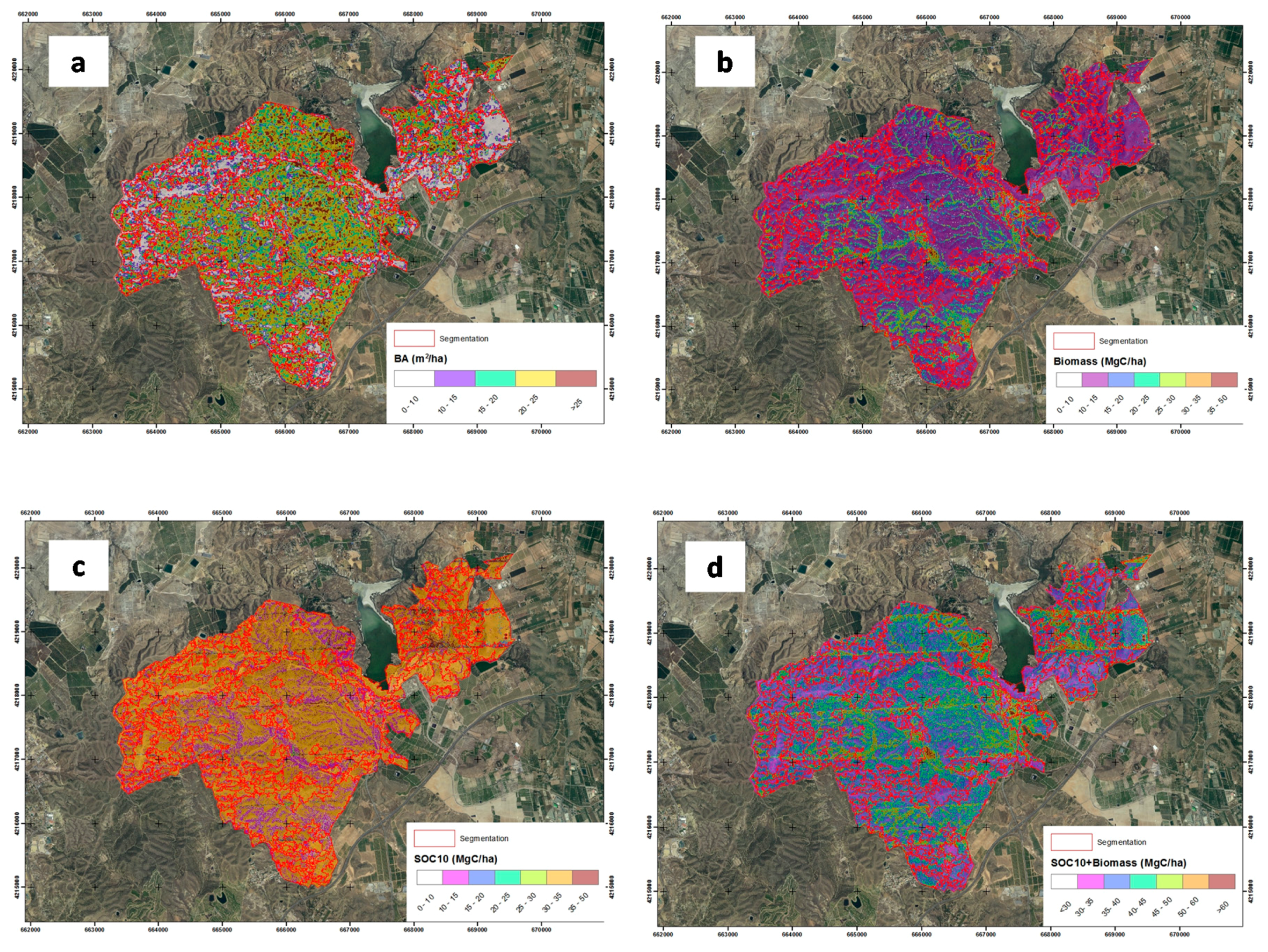
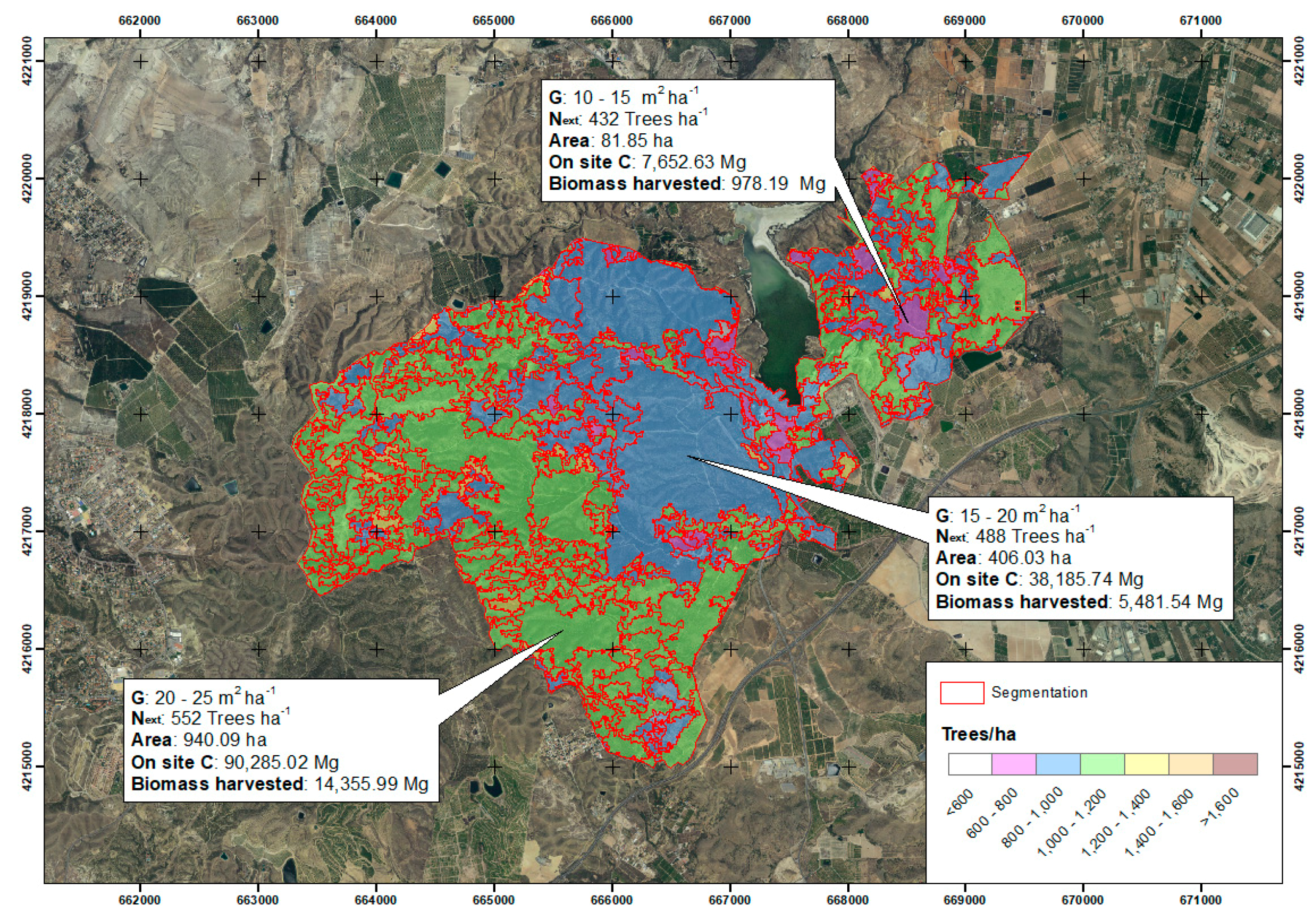
3.3. Cartography of C Stocks and Future Projection under Thinning Treatments

Using OTB and G segmentation, a total of 270 stands were delineated with a spatial radius and a range radius of 2 and a minimum size region of 20 (average stand area = 5.32 ha) (

Table 4. Stands characteristics according to semi-automatic forest stand delineation (Orpheo ToolBox software) and basal area (G) and 10-year C stock projections (biomass and soil organic carbon stock at 0–40 cm soil layer; W_t-S, SOC-S₄₀) of Pinus halepensis plantations at Los Cuadros (Murcia, Spain) under different scenarios.

Categories G (m2 ha−1)	Number of Stands	Mean Area (ha)	Overall Area (ha)	Mean Density (trees ha−1)	Wt-S + SOC-S40
					Current (Mg ha−1)	Ratio (Mg ha−1 year−1, 57 years)	Ten Years Projection without Intervention (Mg) 1	Ten Years Projection with Intervention (Mg) 2	Biomass Harvested (Mg)
0–10	8	0.19	1.53	880	78.89	1.38	141.81	144.07	13.96
10–15	45	1.82	81.85	982	78.33	1.37	7532.65	7652.63	978.19
15–20	101	4.02	406.03	1038	78.77	1.38	37,586.19	38,185.74	5481.54
20–25	111	8.47	940.09	1102	80.43	1.41	88,866.70	90,285.02	14,355.99
>25	5	1.54	7.69	1145	80.04	1.40	723.16	734.68	126.58
Overall	270		1437.20				134,850.54	137,002.16	20,956.28

¹ (Overall area × Current W_t-S + SOC-S₄₀) + (Overall area × Ratio W_t-S + SOC-S₄₀ × 10); ² (Overall area × Current W_t-S + SOC-S₄₀) + (Overall area × Ratio W_t-S + SOC-S₄₀ × 10.107 × 10).

; Figure 5a).

The best kNN models were selected to spatially estimate the C stocks for the study area (MSNPP for biomass, RF for SOC-S₁₀ and MSN2 for W_t-S + SOC-S₁₀, see Figure 2 and Figure 4 and Table 3). Based on the stand cartography and these models, the distribution maps with predicted values of C stocks in the forested area show a mosaic of C stock patterns in the P. halepensis forest (Figure 5b–d). We obtained a mean W_t-S value of 22.73 Mg ha⁻¹ (±8.71 Mg ha⁻¹), ranging from 6.38 Mg ha⁻¹ to 48.10 Mg ha⁻¹, a mean SOC-S₁₀ value of 20.99 Mg ha⁻¹ (±10.22 Mg ha⁻¹), ranging from 4.46 Mg ha⁻¹ to 47.78 Mg ha⁻¹, a mean W_t-S + SOC-S₁₀ value of 41.96 Mg ha⁻¹ (±10.82 Mg ha⁻¹), ranging from 20.14 Mg ha⁻¹ to 77.34 Mg ha⁻¹ and a mean W_t-S + SOC-S₄₀ value of 89.42 Mg ha⁻¹ (±21.59 Mg ha⁻¹), ranging from 57.94 Mg ha⁻¹ to 153.58 Mg ha⁻¹ (Table S3, Supplementary Material).

Starting from the above-mentioned results, the current on-site C stock estimated for the total forested area was 62,834.38 Mg, including 32,667.55 Mg in W_t-S and 30,166.82 Mg in SOC-S₁₀ (corresponding to 230,602.17 Mg CO₂), or 127,867.67 Mg, including 32,667.55 Mg in W_t-S and 95,200.12 Mg in SOC-S₄₀ (corresponding to 469,274.37 Mg CO₂).

Comparison of the C stock per hectare of the plantations would not offer a real figure in relation to the effect of the most efficient silvicultural treatment on the C stock balance. Therefore, we projected the C stock considering the stand delineation and two scenarios: first, a non-intervention scenario and second, considering a heavy thinning program (final density of 550 trees ha⁻¹) for the whole area in the present year. Then, the C stock was quantified by adding the estimated rate of increase in the accumulation in biomass and soil (W_t -SOC-S₄₀) for ten-year projections. Finally, the biomass harvested was also included (Table 4).

The high-density areas (>770 trees ha⁻¹) are comprised of 100% Aleppo pine (Table 4). Under a non-intervention scenario, the mean rate of C stock increase in the next 10 years would be 1.38 Mg ha⁻¹ year⁻¹ and the stands would be able to stock 134,850.54 Mg of C (corresponding to 494,901.49 Mg CO₂); under the intervention scenario, they would be able to stock 137,002.16 Mg of C (corresponding to 502,797.94 Mg CO₂, Table 4). In this latter scenario, the tree density at year 10 would be 550 trees ha⁻¹; so, the biomass stock extraction of the Aleppo pine forest subjected to thinning would represent 20,956.28 Mg of C (corresponding to 76,909.54 Mg CO₂, Table 4) and the overall C stock accumulated in the non-intervention scenario would be 23,107.90 Mg (corresponding to 84,805.99 Mg CO₂). This quantity represents an increment of 17.1% with respect to the non-intervention scenario and has an estimated value in the C market of 1,601,137.09 €.

4. Discussion

Several studies have demonstrated the importance of C stocks estimation in current forest management [60]. Pine plantations in Mediterranean areas are often managed for multi-objective functions, such as soil and water protection, restoration efforts to re-establish native forest cover, social uses [16], and, more recently, for the provision of ecosystem services such as C sinks, both on-site (biomass and soil) and off-site (wood products or bioenergy) [61]. However, many of the Pinus plantations have received little or no silvicultural intervention and are now highly homogenous in terms of composition and age structure. This, together with their high densities and large areas of forested land, requires the application of thinning treatments to maintain their stability [21]. However, the impacts of these treatments on ecosystem C storage and sequestration rates remain poorly described for some Mediterranean species. In this study, we highlight the effect of thinning treatments on C stocks; in particular, SOC-S, which compensates the loss of total biomass as a result of thinning extraction. Moreover, we show that low density ALS data-based inventories can be used to estimate biomass and SOC C stocks for P. halepensis forest plantations in southern Spain, using kNN models. We have confirmed the advantages of using ALS-based inventories to assess total C stocks in pine plantations in semiarid areas and their applicability for planning alternative silvicultural management to optimize C stocks [62,63].

4.1. C stock in Biomass and SOC under Different Thinning Intensities

In line with our first hypothesis, the biomass C stock was significantly higher in control (unthinned) plots—which is consistent with estimates for other Aleppo pine stands in the region that support relatively low basal areas [64,65]; and for other pine species [27,66,67]. Thinning operations involve a loss of total biomass (without including also the biomass that is removed), which results in lower densities and basal areas in thinned stands [27]. In this study, the average biomass C stock calculated for P. halepensis forests ranged between 41.65 Mg ha⁻¹ (unthinned plots) and 13.93 Mg ha⁻¹ (heavy thinning). The former value exceeds those reported for dominant Aleppo pine forests in similar ecological conditions (25.29 Mg ha⁻¹, [68]) and is much higher than in other studies (15.02 Mg ha⁻¹, [14]). These discrepancies can be explained by the inclusion of root biomass (11.42 Mg ha⁻¹ and 4.14 Mg ha⁻¹ for the control and treatment H, respectively) and the structural-silvicultural heterogeneity of the Aleppo pine stands in relation to age and density (1400 trees ha⁻¹ − dbh = 15 cm in this study; 1150 trees ha⁻¹ − dbh = 12 cm and 1200 trees ha⁻¹ − dbh = 20 cm, respectively, in the two cited studies). Moreover, the development of allometric relationships at a national level may limit their application at a local scale [37,69], in particular if the sample sizes are not sufficiently large (i.e., >100 sample trees per species; [70]).

Our second hypothesis was that SOC-S would be higher in the thinned plots and we found significant differences among the thinning intensities. In our study, SOC₄₀-S ranged between 50.18 Mg ha⁻¹ (±2.70 Mg ha⁻¹), for the unthinned treatment and 87.24 Mg ha⁻¹ (±3.1 Mg ha⁻¹), with heavy thinning. These values are higher than those found by [71], who determined an average SOC-S in an Aleppo pine plantation (northern Spain, 300 trees ha⁻¹, dbh = 17.5 cm) of 40.72 Mg ha⁻¹ but lower than those in other studies conducted in Mediterranean pine forests, for which SOC-S ranged between 90 and 166 Mg C ha⁻¹ [72,73,74] in a reforested stand. The high thinning intensity gave the greatest capacity for stocking of SOC₄₀-S (73.8 and 58.66% greater than the control and moderate thinning, respectively). This means an estimated rate of SOC accumulation after thinning, with respect to the unthinned plots, of 2.26 to 2.85 Mg ha⁻¹ year⁻¹ (for M and H thinning, respectively) over a period of 13 years, much higher than that observed by [71], who estimated an average rate of SOC accumulation in P. halepensis forests of 0.50 Mg ha⁻¹ year⁻¹ for a period of 35 years.

These results are contrary to those found in some previous studies, where thinning operations had a non-significant or negative impact on soil C in Mediterranean pine forests [27,29,74] but not to those of other studies [10,66]. Thinning may improve C sequestration through several factors involved in SOC accumulation: variation in the quality and quantity of inputs (litterfall and logging residues), an increase in N use efficiency, protection of both new and old SOC in mineral-associated fractions (<50 μm) and a greater micro-climatic effect on litter decomposition [13,75,76], enhancing long-term storage in the soil [77]. In our study, the shallowest soil layer (0–20 cm) had a higher SOC-S (56% greater on average, among the treatments)—highlighting the role of litter quantity and turnover [75,78], since they directly receive the contribution of litterfall, in which there is greater microbial activity [76], whereas the subsoil SOC is related more to the density of roots [79]. Additionally, some of the thinning residues, such as slashes, were left on-site, thus helping to maintain soil C stocks [80].

These findings support the idea that P. halepensis plantations in degraded semiarid areas can accumulate large amounts of SOC [14]. The forest management, along the 13-year management period, had an impact on the on-site C stock (W_t + SOC₄₀-S), of 9.9% and 10.1% for the M and H thinning treatments, respectively) in comparison to the control, without considering the biomass extracted during thinning operations. Although thinning operations involve a loss of total biomass (without including the biomass removed), which slightly reduces the mitigation capacity of the pine forest after thinning, when the net balance between biomass and SOC₄₀–S is calculated, it is evident that moderate and heavy thinning are more efficient silvicultural alternatives for C sequestration, contributing to the forest management that is most suitable for C sequestration [67,81].

4.2. Low Density ALS Data and the C Stock in Biomass and SOC

In recent years, ALS sensors have been used mainly for the determination of forest parameters, being a critical technology for forest inventory and management [82]. Several studies have shown the usefulness of ALS data for estimating forest variables in Mediterranean pine plantations [83,84], as well as volume [15].

According to the kNN models generated, with the use of height percentiles (H_P₆₀, H_P₉₉) and another parameter concerning the horizontal distribution of the point cloud (i.e., the canopy density or the percentage of returns above a certain height threshold), the ALS-derived metric was able to generate accurate information on biomass and soil C stocks in fairly homogeneous forests of P. halepensis plantations. [15] modelled the volume in a P. halepensis plantation using low density ALS data (1 point m⁻²), as in this study and concluded that the best models were developed using the metrics H_P₉₅ and all returns above 1 m (R² = 0.89, RMSE = 11.01 m³ ha⁻¹). We found that W_t-S was the variable predicted with the highest precision (R² = 0.82, RMSN = 8.03 Mg ha⁻¹, MSNPP model). These values of R² lie within the range reported in the literature for biomass estimations for coniferous species (from 0.46 to 0.97; [32,34,45,46,83,85,86,87]). For SOC-S, the models obtained for SOC-S₁₀ (R² = 0.82, RMSE = 9.93 Mg ha⁻¹; RF model) were better than those for SOC-S₄₀ (R² = 0.47, RMSE = 9.08 Mg ha⁻¹; MSNPP model). Nonparametric techniques, such as kNN algorithms, have been used frequently to generate spatially-explicit forest biomass models using ALS and inventory data [48,88] but little research has been performed about the use of kNN regression models for C stock estimations in comparison to traditional linear regression methods [89]. However, kNN is a very simple classifier that works well in basic recognition problems and normality is not needed to obtain robust and understandable models [48].

The main sources of error in our study are the use of low-resolution ALS data, the time delay among ALS signals and the limited number of ground plots. Low density ALS data are often used to cover large study areas [46,63], sometimes with less than 1 point m², without significant loss of information for the mean and dominant height, stand basal area, stand volume and stand biomass fractions. However, the use of low density ALS data may lead to an underestimation of tree height [15,62] and consequently errors in biomass estimation. On the other hand, low density ALS data have many advantages, given their accuracy, ability to be extrapolated to the whole area of study and combination with field data to provide biomass and soil C stocks data at the forest stand scale [63]. In this sense, our results show that the estimated variables can be modelled with good precision for the estimation of the C stocks variables of P. halepensis forests using low resolution ALS (pulse density 1 point m⁻²), as observed also in previous studies [68]. The time delay between the ALS data acquisition and the field data collection (i.e., the 5–8 years) was not considered a significant source of error as has been shown in previous works [68] and for the low growth rate of pine forest under study during that period (mean annual increment 1.7 mm year⁻¹). The limited number of ground plots and the consequent lack of stratification by density type are also possible sources of error. However, the accuracy of our LiDAR-based inventory at the stand level was comparable to that of traditional stand examinations for structural attributes and the LiDAR data were able to provide information across a much larger area than the stand examinations alone.

4.3. Cartography of C Stocks and Management Implications

Finally, we created a set of C stock maps of P. halepensis forests at a pixel scale (18 × 18 m) to describe the spatial pattern of the C stock (Figure 6). The MSN model was selected to spatially estimate the C stock for the study area. Our estimates of W_t-S + SOC₄₀-S ranged from 57.94 to 153.58 Mg ha⁻¹, averaging 89.42 Mg ha⁻¹ and showing low growth rates and thus small C stocks in comparison with other Pinus species [27]. When the net balance of C absorptions is calculated, it is evident that the plantations managed with heavy thinning are more efficient than the unmanaged forests, especially when the SOC₄₀-S sequestration is considered. A possible increment in the net annual C sequestration could be achieved by increasing the thinning operations. Our results outline the important role that silviculture plays in augmenting the C sink; but, forest planning could alter the potential C accumulation in the coming years. Under a non-intervention scenario, C sequestration would be 505,323.51 Mg CO₂, a little below that of the intervention scenario (513,829.76 Mg CO₂, Table 4). However, when the harvested biomass is included the overall C stock accumulated during the non-intervention scenario would be 290,764.26 Mg CO₂. This quantity represents an increment of 57.5% with respect to the non-intervention scenario. Thus, given the substantial contribution of silviculture to C sequestration, its implementation must be encouraged to counter atmospheric CO₂ emissions [27,29,71].

In Mediterranean areas, despite the fact that the area of forest increased notably in the 20th century thanks to pine plantations, efforts should now focus on silviculture rather than on expanding new pine plantations. This target should be included in the silvicultural strategy of P. halepensis pine forests in semiarid areas, thus ensuring the maintenance of ecosystem services related to seminatural forests. Mature Aleppo pine stands are often harvested for protection and conservation purposes, which should include on-site C sequestration in long-lived pools, as well as continued exports of C for potential off-site offsets such as bioenergy, as has been observed for other Mediterranean species [29]. One way to estimate the economic value underlying C sequestration is based on the CO₂ stock exchange [90]. One tonne of CO₂ is quoted at 12.97 € in the European Union Emission Trading (averaged monthly value for the year 2018). The economic value of C sequestration in the area under study would, therefore, be 3,771,212.45 € in the intervention scenario. This amount may make a considerable contribution to ecosystem service maintenance and woodland conservation if returned to the local municipalities as payment for environmental services, as subsidies and incentives to the local society and stakeholders to preserve the services provided by the local ecosystems [91]. Additionally, thinning offers other benefits—such as improving biodiversity, resilience against disturbances (fire, pests and diseases, droughts) and the quality of wood products—in the face of climate change [17,27,92].

To support this forest management plan, our results show that accurate mapping of the P. halepensis C stock distribution can be modelled with good precision using low resolution ALS (pulse density 0.5–1 points m⁻²) and a limited number of field measurements, as observed in previous studies [68]. Although this paper presents a case study of a spatially-explicit estimation of on-site C stocks in southern Spain, the methodology can be generalized to plantations of other Mediterranean pine species with similar site characteristics within the Mediterranean Basin, with low errors (RMSE) and high correlation values. The detailed cartography achieved with low density ALS data is useful to prescribe land management activities at the local level. Recently, the cost of ALS data acquisition has decreased [93,94]—it can be obtained for free in some countries (e.g., in Spain, 0.5–1.0 points m⁻²) and is comparable to or even less than the cost of large-scale field data collection [95]. As a consequence, considering the improvement achieved by using ALS-derived products for estimating and mapping C stocks, it may be a better alternative for forest managers.

5. Conclusions

The comparison of three different thinning intensities, in terms of the on-site C stock after 13 years, has shown that heavy thinning gave the highest efficiency with regard to C sequestration. The thinning treatments produced a loss of total biomass but an interesting increase in C storage in the soil, even though the tree density at year 13 in the heavily thinned plots was approximately one half that of the unmanaged plantation. With proper management, this potential could be used to increase C sequestration in dry P. halepensis forests of the Mediterranean Basin. This study also verifies the usefulness of low density PNOA-ALS data to accurately estimate on-site C stocks in a monospecific Aleppo pine forest; these data permit the computation of C sequestration and the adaptation of forest management at regional scales, reducing forest inventory costs. The use of non-parametric methods is especially interesting to improve forest parameters modelling. The kNN algorithm was applied to improve the predictions and it confirmed the gain achieved using standardizing spectral distances. The kNN modelling approach reinforced our confidence in the quality of our estimates, although the differences were generally much greater for models including SOC.

The cartography obtained represents a reliable picture of the current situation of C stocks pools in Aleppo pine plantations. This high-resolution raster map of predicted C stocks is useful for silvicultural planning and future monitoring of potential changes in this area, which represent important contributions to the preliminary assessment of potential benefits in terms of C sequestration in forests due to sustainable silvicultural practices. Considering a thinning plan in a specific geographical location, that covers around 1400 ha in southern Spain, it was possible to quantify the net C sequestration for a 10-year plan. These C credits could be valued within the Voluntary Market by commercial and non-profit organizations, local administrations and even individuals, in order to offset, completely or partially, the emissions for which they are responsible. This assessment can help forest managers to make better informed decisions regarding silviculture oriented to increase C sequestration rates.

References

1. Parmesan, C.; Yohe, G. A Globally Coherent Fingerprint of Climate Change Impacts across Natural Systems. Nature 2003, 421, 37–42. [Google Scholar] [CrossRef] [PubMed]
2. Matthews, H.D.; Kirsten, Z.; Reto, K.; Myles, R.A. Focus on Cumulative Emissions, Global Carbon Budgets and the Implications for Climate Mitigation Targets. Environ. Res. Lett. 2018, 13, 010201. [Google Scholar] [CrossRef]
3. Pan, Y.; Birdsey, R.A.; Fang, J.; Houghton, R.; Kauppi, P.E.; Kurz, W.A.; Phillips, O.L.; Shvidenko, A.; Lewis, S.L.; Canadell, J.G.; et al. A Large and Persistent Carbon Sink in the World’s Forests. Science 2011, 333, 988–993. [Google Scholar] [CrossRef] [PubMed]
4. Bellassen, V.; Luyssaert, S. Carbon Sequestration: Managing Forests in Uncertain Times. Nature 2014, 506, 153–155. [Google Scholar] [CrossRef] [PubMed]
5. Waring, R.H.; Running, S.W. Chapter 3—Carbon Cycle. In Forest Ecosystems, 3rd ed.; Academic Press: San Diego, CA, USA, 2007; pp. 59–98. [Google Scholar]
6. Lal, R.; Wakene, N.; Klaus, L. Carbon Sequestration in Soil. Curr. Opin. Environ. Sustain. 2015, 15, 79–86. [Google Scholar] [CrossRef]
7. Wäldchen, J.; Schulze, E.-D.; Schöning, I.; Schrumpf, M.; Sierra, C. The Influence of Changes in Forest Management over the Past 200 Years on Present Soil Organic Carbon Stocks. For. Ecol. Manag. 2013, 289, 243–254. [Google Scholar] [CrossRef]
8. Fahey, T.J.; Woodbury, P.B.; Battles, J.J.; Goodale, C.L.; Hamburg, S.P.; Ollinger, S.V.; Woodall, C.W. Forest Carbon Storage: Ecology, Management, and Policy. Front. Ecol. Environ. 2009, 8, 245–252. [Google Scholar] [CrossRef]
9. Vilà-Cabrera, A.; Coll, L.; Martínez-Vilalta, J.; Retana, J. Forest Management for Adaptation to Climate Change in the Mediterranean Basin: A Synthesis of Evidence. For. Ecol. Manag. 2018, 407, 16–22. [Google Scholar] [CrossRef]
10. Kim, S.; Kim, C.; Han, S.H.; Lee, S.; Son, Y. A Multi-Site Approach toward Assessing the Effect of Thinning on Soil Carbon Contents across Temperate Pine, Oak, and Larch Forests. For. Ecol. Manag. 2018, 424, 62–70. [Google Scholar] [CrossRef]
11. Bottcher, H.; Lindner, M. Managing Forest Plantations for Carbon Sequestration Today and in the Future. In Ecosystem Goods and Services from Plantation Forests; Bauhaus, J., van der Meer, P., Kanninen, M., Eds.; Earthscan: London, UK, 2010. [Google Scholar]
12. Rötzer, T.; Dieler, J.; Mette, T.; Moshammer, R.; Pretzsch, H. Productivity and Carbon Dynamics in Managed Central European Forests Depending on Site Conditions and Thinning Regimes. For. Int. J. For. Res. 2010, 83, 483–496. [Google Scholar] [CrossRef]
13. Segura, C.; Jiménez, M.N.; Nieto, O.; Navarro, F.B.; Fernández-Ondoño, E. Changes in Soil Organic Carbon over 20 Years after Afforestation in Semiarid Se Spain. For. Ecol. Manag. 2016, 381, 268–278. [Google Scholar] [CrossRef]
14. Sanchez Pellicer, T.; Alcón, S.M.; Morán, J.L.T.; Navarro, J.A.; Fernández-Landa, A. Forestco2: Monitorización De Sumideros De Carbono En Masas De Pinus Halepensis En La Región De Murcia. Available online: https://www.aet2017.es/ (accessed on 19 October 2018).
15. Montealegre, A.L.; Lamelas, M.T.; de la Riva, J.; García-Martín, A.; Escribano, F. Use of Low Point Density Als Data to Estimate Stand-Level Structural Variables in Mediterranean Aleppo Pine Forest. For. Int. J. For. Res. 2016, 89, 373–382. [Google Scholar] [CrossRef]
16. Pausas, J.G.; Bladé, C.; Valdecantos, A.; Seva, J.P.; Fuentes, D.; Alloza, J.A.; Vilagrosa, A.; Bautista, S.; Cortina, J.; Vallejo, R. Pines and Oaks in the Restoration of Mediterranean Landscapes of Spain: New Perspectives for an Old Practice—A Review. Plant Ecol. 2004, 171, 209–220. [Google Scholar] [CrossRef]
17. Moreno-Gutiérrez, C.; Barberá, G.G.; Nicolás, E.; de Luis, M.; Castillo, V.M.; Martínez-Fernández, F.; Querejeta, J.I. Leaf Δ18o of Remaining Trees Is Affected by Thinning Intensity in a Semiarid Pine Forest. Plant Cell Environ. 2011, 34, 1009–1019. [Google Scholar] [CrossRef] [PubMed]
18. Olivar, J.; Bogino, S.; Rathgeber, C.; Bonnesoeur, V.; Bravo, F. Thinning Has a Positive Effect on Growth Dynamics and Growth–Climate Relationships in Aleppo Pine (Pinus Halepensis) Trees of Different Crown Classes. Ann. For. Sci. 2014, 71, 395–404. [Google Scholar] [CrossRef]
19. Alfaro-Sánchez, R.; López-Serrano, F.R.; Rubio, E.; Sánchez-Salguero, R.; Moya, D.; Hernández-Tecles, E.; de las Heras, J. Response of Biomass Allocation Patterns to Thinning in Pinus Halepensis Differs under Dry and Semiarid Mediterranean Climates. Ann. For. Sci. 2015, 72, 595–607. [Google Scholar] [CrossRef]
20. Giuggiola, A.; Ogée, J.; Rigling, A.; Gessler, A.; Bugmann, H.; Treydte, K. Improvement of Water and Light Availability after Thinning at a Xeric Site: Which Matters More? A Dual Isotope Approach. New Phytol. 2016, 210, 108–121. [Google Scholar] [CrossRef] [PubMed]
21. Serrada, R.; González, G.M. Compendio De Selvicultura Aplicada En España; Instituto Nacional de Investigación y Tecnología Agraria y Alimentaria: Madrid, Spain, 2008. [Google Scholar]
22. Ruiz-Peinado, R.; Bravo-Oviedo, A.; Montero, G.; del Río, M. Carbon Stocks in a Scots Pine Afforestation under Different Thinning Intensities Management. Mitig. Adapt. Strat. Glob. Chang. 2016, 21, 1059–1072. [Google Scholar] [CrossRef]
23. Bravo, F.; Bravo-Oviedo, A.; Diaz-Balteiro, L. Carbon Sequestration in Spanish Mediterranean Forests under Two Management Alternatives: A Modeling Approach. Eur. J. For. Res. 2008, 127, 225–234. [Google Scholar] [CrossRef]
24. Pérez-Cruzado, C.; Mohren, G.M.J.; Merino, A.; Rodríguez-Soalleiro, R. Carbon Balance for Different Management Practices for Fast Growing Tree Species Planted on Former Pastureland in Southern Europe: A Case Study Using the Co2fix Model. Eur. J. For. Res. 2012, 131, 1695–1716. [Google Scholar] [CrossRef]
25. Herrero, C.; Bravo, F. Can We Get an Operational Indicator of Forest Carbon Sequestration? A Case Study from Two Forest Regions in Spain. Ecol. Indic. 2012, 17, 120–126. [Google Scholar] [CrossRef]
26. Padilla, F.M.; Vidal, B.; Sánchez, J.; Pugnaire, F.I. Land-Use Changes and Carbon Sequestration through the Twentieth Century in a Mediterranean Mountain Ecosystem: Implications for Land Management. J. Environ. Manag. 2010, 91, 2688–2695. [Google Scholar] [CrossRef] [PubMed]
27. Ruiz-Peinado, R.; Bravo-Oviedo, A.; Lopez-Senespleda, E.; Bravo, F.; del Rio, M. Forest Management and Carbon Sequestration in the Mediterranean Region: A Review. For. Syst. 2017, 26. [Google Scholar] [CrossRef]
28. Næsset, E. Practical Large-Scale Forest Stand Inventory Using a Small-Footprint Airborne Scanning Laser. Scand. J. For. Res. 2004, 19, 164–179. [Google Scholar] [CrossRef]
29. Del Río, M.; Calama, R.; Cañellas, I.; Roig, S.; Montero, G. Thinning Intensity and Growth Response in Sw-European Scots Pine Stands. Ann. For. Sci. 2008, 65, 308. [Google Scholar] [CrossRef]
30. Næsset, E. Predicting Forest Stand Characteristics with Airborne Scanning Laser Using a Practical Two-Stage Procedure and Field Data. Remote. Sens. Environ. 2002, 80, 88–99. [Google Scholar] [CrossRef]
31. Hall, S.A.; Burke, I.C.; Box, D.O.; Kaufmann, M.R.; Stoker, J.M. Estimating Stand Structure Using Discrete-Return Lidar: An Example from Low Density, Fire Prone Ponderosa Pine Forests. For. Ecol. Manag. 2005, 208, 189–209. [Google Scholar] [CrossRef]
32. Watt, P.; Watt, M.S. Development of a National Model of Pinus Radiata Stand Volume from Lidar Metrics for New Zealand. Int. J. Remote. Sens. 2013, 34, 5892–5904. [Google Scholar] [CrossRef]
33. Kukunda, C.B.; Duque-Lazo, J.; González-Ferreiro, E.; Thaden, H.; Kleinn, C. Ensemble Classification of Individual Pinus Crowns from Multispectral Satellite Imagery and Airborne Lidar. Int. J. Appl. Earth Obs. Geoinf. 2018, 65, 12–23. [Google Scholar] [CrossRef]
34. McRoberts, R.E.; Næsset, E.; Gobakken, T.; Bollandsås, O.M. Indirect and Direct Estimation of Forest Biomass Change Using Forest Inventory and Airborne Laser Scanning Data. Remote Sens. Environ. 2015, 164, 36–42. [Google Scholar] [CrossRef]
35. Chirici, G.; Mura, M.; McInerney, D.; Py, N.; Tomppo, E.O.; Waser, L.T.; Travaglini, D.; McRoberts, R.E. A Meta-Analysis and Review of the Literature on the K-Nearest Neighbors Technique for Forestry Applications That Use Remotely Sensed Data. Remote Sens. Environ. 2016, 176, 282–294. [Google Scholar] [CrossRef]
36. Alías, L.J.; Ortiz, R.; Sánchez, A.; Linares, P.; Martínez, M.J.; Marín, P. Memoria Y Mapa De Suelos Escala 1:100.000 Hoja Número 913 (Orihuela); Universidad de Murcia y Dirección General de Conservación de la Naturaleza, Ministerio de Medio Ambiente: Murcia, Spain, 1998. [Google Scholar]
37. Ruiz-Peinado, R.; del Rio, M.; Montero, G. New Models for Estimating the Carbon Sink Capacity of Spanish Softwood Species. For. Syst. 2011, 20, 176–188. [Google Scholar] [CrossRef]
38. Penman, J.; Gytarsky, M.; Hiraishi, T.; Krug, T.; Kurger, D.; Pipatti, R.; Buendia, L.; Miwa, K.; Ngara, T.; Tanabe, K. Good Practice Guidance for Land Use, Land-Use Change and Forestry; Institute for Global Environmental Strategies for the Intergovernmental Panel on Climate Change: Hayama, Japan, 2003. [Google Scholar]
39. Nelson, D.W.; Sommers, L.E. Total Carbon, Organic Carbon, and Organic Matter. Methods Soil Anal. Part 3 Chem. Methods 1996, 3, 961–1010. [Google Scholar]
40. Post, W.M.; Kwon, K.C. Soil Carbon Sequestration and Land-Use Change: Processes and Potential. Glob. Chang. Boil. 2000, 6, 317–327. [Google Scholar] [CrossRef]
41. Mann, L.K. Changes in Soil Carbon Storage after Cultivation. Soil Sci. 1986, 142, 279–288. [Google Scholar] [CrossRef]
42. Farina, R.; Marchetti, A.; Francaviglia, R.; Napoli, R.; di Bene, C. Modeling Regional Soil C Stocks and Co2 Emissions under Mediterranean Cropping Systems and Soil Types. Agric. Ecosyst. Environ. 2017, 238, 128–141. [Google Scholar] [CrossRef]
43. IGN. Plan Nacional De Ortografía Aérea. Instituto Geográfico Nacional. Available online: http://pnoa.ign.es/ (accessed on 5 May 2017).
44. McGaughey, R.J. Fusion/Ldv: Software for Lidar Data Analysis and Visualization; US Department of Agriculture, Forest Service, Pacific Northwest Research Station: Seattle, WA, USA, 2009; Volume 123.
45. Næsset, E.; Gobakken, T. Estimation of above- and Below-Ground Biomass across Regions of the Boreal Forest Zone Using Airborne Laser. Remote Sens. Environ. 2008, 112, 3079–3090. [Google Scholar] [CrossRef]
46. González-Ferreiro, E.; Diéguez-Aranda, U.; Miranda, D. Estimation of Stand Variables in Pinus Radiata D. Don Plantations Using Different Lidar Pulse Densities. Forestry 2012, 85, 281–292. [Google Scholar] [CrossRef]
47. Sokal, R.R.; Rohlf, F.J. Biometry; W.H. Freeman and Co.: New York, NY, USA, 1995. [Google Scholar]
48. Breidenbach, J.; Næsset, E.; Gobakken, T. Improving K-Nearest Neighbor Predictions in Forest Inventories by Combining High and Low Density Airborne Laser Scanning Data. Remote Sens. Environ. 2012, 117, 358–365. [Google Scholar] [CrossRef]
49. Crookston, N.; Finley, A. Yaimpute: An R Package for Knn Imputation. J. Stat. Softw. 2008, 23, 1–16. [Google Scholar] [CrossRef]
50. Packalén, P.; Maltamo, M. The K-Msn Method for the Prediction of Species-Specific Stand Attributes Using Airborne Laser Scanning and Aerial Photographs. Remote Sens. Environ. 2007, 109, 328–341. [Google Scholar] [CrossRef]
51. Valbuena, R.; Vauhkonen, J.; Packalen, P.; Pitkänen, J.; Maltamo, M. Comparison of Airborne Laser Scanning Methods for Estimating Forest Structure Indicators Based on Lorenz Curves. Isprs J. Photogramm. Remote Sens. 2014, 95, 23–33. [Google Scholar] [CrossRef]
52. McRoberts, R.E.; Nelson, M.D.; Wendt, D.G. Stratified Estimation of Forest Area Using Satellite Imagery, Inventory Data, and the K-Nearest Neighbors Technique. Remote Sens. Environ. 2002, 82, 457–468. [Google Scholar] [CrossRef]
53. R Development Core Team. R: A Language and Environment for Statistical Computing. R Foundation for Statistical Computing; R Foundation for Statistical Computing: Vienna, Austria, 2011. [Google Scholar]
54. Usdm: Uncertainty Analysis for Species Distribution Models. R Package Version 1.1-8. 2017. Available online: https://rdrr.io/cran/usdm/ (accessed on 17 October 2018).
55. Grizonnet, M.; Michel, J.; Poughon, V.; Inglada, J.; Savinaud, M.; Cresson, R. Orfeo Toolbox: Open Source Processing of Remote Sensing Images. Open Geospat. Data Softw. Stand. 2017, 2, 15. [Google Scholar] [CrossRef]
56. Babich, G.A.; Camps, O.I. Weighted Parzen Windows for Pattern Classification. IEEE Trans. Pattern Anal Mach. Intell. 1996, 18, 567–570. [Google Scholar] [CrossRef]
57. Wu, Z.; Heikkinen, V.; Hauta-Kasari, M.; Parkkinen, J.; Tokola, T. Als Data Based Forest Stand Delineation with a Coarse-to-Fine Segmentation Approach. In Proceedings of the 2014 7th International Congress on Image and Signal Processing, Dalian, China, 14–16 October 2014. [Google Scholar]
58. Kathuria, A.; Turner, R.; Stone, C.; Duque-Lazo, J.; West, R. Development of an Automated Individual Tree Detection Model Using Point Cloud Lidar Data for Accurate Tree Counts in a Pinus Radiata Plantation. Aust. For. 2016, 79, 126–136. [Google Scholar] [CrossRef]
59. Varo-Martínez, M.Á.; Navarro-Cerrillo, R.M.; Hernández-Clemente, R.; Duque-Lazo, J. Semi-Automated Stand Delineation in Mediterranean Pinus Sylvestris Plantations through Segmentation of Lidar Data: The Influence of Pulse Density. Int. J. Appl. Earth Obs. Geoinf. 2017, 56, 54–64. [Google Scholar] [CrossRef]
60. Metsaranta, J.M.; Shaw, C.H.; Kurz, W.A.; Boisvenue, C.; Morken, S. Uncertainty of Inventory-Based Estimates of the Carbon Dynamics of Canada’s Managed Forest (1990–2014). Can. J. For. Res. 2017, 47, 1082–1094. [Google Scholar] [CrossRef]
61. Peñuelas, J.; Sardans, J.; Filella, I.; Estiarte, M.; Llusià, J.; Ogaya, R.; Carnicer, J.; Bartrons, M.; Rivas-Ubach, A.; Grau, O.; et al. Impacts of Global Change on Mediterranean Forests and Their Services. Forests 2017, 8, 463. [Google Scholar] [CrossRef]
62. Vosselman, G.; Maas, H.-G. Airborne and Terrestrial Laser Scanning; Whittles Publishing: Dunbeath, UK, 2010. [Google Scholar]
63. Maltamo, M.; Næsset, E.; Vauhkonen, J. Forestry Applications of Airborne Laser Scanning: Concepts Case Studies; Springer: Dordrecht, The Netherlands, 2014; Volume 27, p. 460. [Google Scholar]
64. Molina, A.J.; del Campo, A.D. The Effects of Experimental Thinning on Throughfall and Stemflow: A Contribution towards Hydrology-Oriented Silviculture in Aleppo Pine Plantations. For. Ecol. Manag. 2012, 269, 206–213. [Google Scholar] [CrossRef]
65. De las Heras, J.; Moya, D.; López-Serrano, F.R.; Rubio, E. Carbon Sequestration of Naturally Regenerated Aleppo Pine Stands in Response to Early Thinning. New For. 2013, 44, 457–470. [Google Scholar] [CrossRef]
66. Bravo-Oviedo, A.; Ruiz-Peinado, R.; Modrego, P.; Alonso, R.; Montero, G. Forest Thinning Impact on Carbon Stock and Soil Condition in Southern European Populations of P. Sylvestris L. For. Ecol. Manag. 2015, 357, 259–267. [Google Scholar] [CrossRef]
67. Del Río, M.; Bravo-Oviedo, A.; Pretzsch, H.; Löf, M.; Ruiz-Peinado, R. A Review of Thinning Effects on Scots Pine Stands: From Growth and Yield to New Challenges under Global Change. For. Syst. 2017, 26. [Google Scholar] [CrossRef]
68. Montealegre, A.L.; Lamelas, M.T.; de la Riva, J.; García-Martín, A.; Escribano, F. Assessment of Biomass and Carbon Content in a Mediterranean Aleppo Pine Forest Using Als Data. 2015. Available online: https://bit.ly/2J2cCCJ (accessed on 17 October 2018).
69. Lambert, M.C.; Ung, C.H.; Raulier, F. Canadian National Tree Aboveground Biomass Equations. Can. J. For. Res. 2005, 35, 1996–2018. [Google Scholar] [CrossRef]
70. McRoberts, R.E.; Westfall, J.A. Effects of Uncertainty in Model Predictions of Individual Tree Volume on Large Area Volume Estimates. For. Sci. 2014, 60, 34–42. [Google Scholar] [CrossRef]
71. Grünzweig, J.M.; Gelfand, I.; Yakir, D. Biogeochemical Factors Contributing to Enhanced Carbon Storage Following Afforestation of a Semi-Arid Shrubland. Biogeosciences 2007, 4, 2111–2145. [Google Scholar] [CrossRef]
72. Díaz-Pinés, E.; Rubio, A.; van Miegroet, H.; Montes, F.; Benito, M. Does Tree Species Composition Control Soil Organic Carbon Pools in Mediterranean Mountain Forests? For. Ecol. Manag. 2011, 262, 1895–1904. [Google Scholar] [CrossRef]
73. Charro, E.; Gallardo, J.F.; Moyano, A. Degradability of Soils under Oak and Pine in Central Spain. Eur. J. For. Res. 2010, 129, 83–91. [Google Scholar] [CrossRef]
74. Ruiz-Peinado, R.; Bravo-Oviedo, A.; López-Senespleda, E.; Montero, G.; Río, M. Do Thinnings Influence Biomass and Soil Carbon Stocks in Mediterranean Maritime Pinewoods? Eur. J. For. Res. 2013, 132, 253–262. [Google Scholar] [CrossRef]
75. Jiménez, M.N.; Navarro, F.B. Thinning Effects on Litterfall Remaining after 8 Years and Improved Stand Resilience in Aleppo Pine Afforestation (Se Spain). J. Environ. Manag. 2016, 169, 174–183. [Google Scholar] [CrossRef] [PubMed]
76. Skovsgaard, J.P.; Stupak, I.; Vesterdal, L. Distribution of Biomass and Carbon in Even-Aged Stands of Norway Spruce (Picea Abies (L.) Karst.): A Case Study on Spacing and Thinning Effects in Northern Denmark. Scand. J. For. Res. 2006, 21, 470–488. [Google Scholar] [CrossRef]
77. Del Galdo, I.; Six, J.; Peressotti, A.; Cotrufo, M.F. Assessing the Impact of Land-Use Change on Soil C Sequestration in Agricultural Soils by Means of Organic Matter Fractionation and Stable C Isotopes. Glob. Chang. Boil. 2003, 9, 1204–1213. [Google Scholar] [CrossRef]
78. Roig, S.; del Río, M.; Cañellas, I.; Montero, G. Litter Fall in Mediterranean Pinus Pinaster Ait. Stands under Different Thinning Regimes. For. Ecol. Manag. 2005, 206, 179–190. [Google Scholar] [CrossRef]
79. Rumpel, C.; Kögel-Knabner, I. Deep Soil Organic Matter—A Key but Poorly Understood Component of Terrestrial C Cycle. Plant Soil 2011, 338, 143–158. [Google Scholar] [CrossRef]
80. Page-Dumroese, D.S.; Jurgensen, M.; Terry, T. Maintaining Soil Productivity during Forest or Biomass-to-Energy Thinning Harvests in the Western United States. West. J. Appl. For. 2010, 25, 5–11. [Google Scholar]
81. Fortin, M.; Ningre, F.; Robert, N.; Mothe, F. Quantifying the Impact of Forest Management on the Carbon Balance of the Forest-Wood Product Chain: A Case Study Applied to Even-Aged Oak Stands in France. For. Ecol. Manag. 2012, 279, 176–188. [Google Scholar] [CrossRef]
82. Wulder, M.A.; White, J.C.; Nelson, R.F.; Næsset, E.; Ørka, H.O.; Coops, N.C.; Hilker, T.; Bater, C.W.; Gobakken, T. Lidar Sampling for Large-Area Forest Characterization: A Review. Remote Sens. Environ. 2012, 121, 196–209. [Google Scholar] [CrossRef]
83. García, M.; Riaño, D.; Chuvieco, E.; Danson, F.M. Estimating Biomass Carbon Stocks for a Mediterranean Forest in Central Spain Using Lidar Height and Intensity Data. Remote Sens. Environ. 2010, 114, 816–830. [Google Scholar] [CrossRef]
84. Navarro-Cerrillo, R.M.; González-Ferreiro, E.; García-Gutiérrez, J.; Ruiz, C.J.C.; Hernández-Clemente, R. Impact of Plot Size and Model Selection on Forest Biomass Estimation Using Airborne Lidar: A Case Study of Pine Plantations in Southern Spain. J. For. Sci. 2017, 63, 88–97. [Google Scholar]
85. Li, Y.; Andersen, Ha.; McGaughey, R. A Comparison of Statistical Methods for Estimating Forest Biomass from Light Detection and Ranging Data. West. J. Appl. For. 2008, 23, 223–231. [Google Scholar]
86. Næsset, E.; Gobakken, T.; Holmgren, J.; Hyyppä, H.; Hyyppä, J.; Maltamo, M.; Nilsson, M.; Olsson, H.; Persson, Å.; Söderman, U. Laser Scanning of Forest Resources: The Nordic Experience. Scand. J. For. Res. 2004, 19, 482–499. [Google Scholar] [CrossRef]
87. Watt, M.S.; Meredith, A.; Watt, P.; Gunn, A. Use of Lidar to Estimate Stand Characteristics for Thinning Operations in Young Douglas-Fir Plantations. N. Z. J. For. Sci. 2013, 43, 18. [Google Scholar] [CrossRef]
88. Domingo, D.; Lamelas, M.; Montealegre, A.; García-Martín, A.; de la Riva, J. Estimation of Total Biomass in Aleppo Pine Forest Stands Applying Parametric and Nonparametric Methods to Low-Density Airborne Laser Scanning Data. Forests 2018, 9, 158. [Google Scholar] [CrossRef]
89. Suchenwirth, L.; Stümer, W.; Schmidt, T.; Förster, M.; Kleinschmit, B. Large-Scale Mapping of Carbon Stocks in Riparian Forests with Self-Organizing Maps and the K-Nearest-Neighbor Algorithm. Forests 2014, 5, 1635–1652. [Google Scholar] [CrossRef]
90. Robertson, K.; Loza-Balbuena, I.; Ford-Robertson, J. Monitoring and Economic Factors Affecting the Economic Viability of Afforestation for Carbon Sequestration Projects. Environ. Sci. Policy 2004, 7, 465–475. [Google Scholar] [CrossRef]
91. Turpie, J.K.; Marais, C.; Blignaut, J.N. The Working for Water Programme: Evolution of a Payments for Ecosystem Services Mechanism That Addresses Both Poverty and Ecosystem Service Delivery in South Africa. Ecol. Econ. 2008, 65, 788–798. [Google Scholar] [CrossRef]
92. Sohn, J.A.; Saha, S.; Bauhus, J. Potential of Forest Thinning to Mitigate Drought Stress: A Meta-Analysis. For. Ecol. Manag. 2016, 380, 261–273. [Google Scholar] [CrossRef]
93. Tilley, B.K.; Munn, I.A.; Evans, D.L.; Parker, R.C.; Roberts, S.D. Cost Considerations of Using Lidar for Timber Inventory. 2004. Available online: https://bit.ly/2NLXoCN (accessed on 17 October 2018).
94. Bergseng, E.; Ørka, H.O.; Næsset, E.; Gobakken, T. Assessing Forest Inventory Information Obtained from Different Inventory Approaches and Remote Sensing Data Sources. Ann. For. Sci. 2015, 72, 33–45. [Google Scholar] [CrossRef]
95. Jakubowski, M.K.; Guo, Q.; Kelly, M. Tradeoffs between Lidar Pulse Density and Forest Measurement Accuracy. Remote Sens. Environ. 2013, 130, 245–253. [Google Scholar] [CrossRef]
Figure 1. Flowchart describing the methodological steps to assess on-site carbon stocks using low density ALS data.
Remotesensing 10 01660 g001
Figure 2. Bivariate relationships between the LiDAR metrics and biomass C stock of Pinus halepensis plantations at Los Cuadros (Murcia, Spain). In all figures, the linear 1:1 line has been fitted. For these equations, the R2 value is included (see Table 3 for RMSE values).
Remotesensing 10 01660 g002
Figure 3. Bivariate relationships between the LiDAR metrics and SOC10 (0–10 cm soil layer) C stock biomass of Pinus halepensis plantations at Los Cuadros (Murcia, Spain). In all figures, the linear 1:1 line has been fitted. For these equations, the R2 value is included (see Table 3 for RMSE values).
Remotesensing 10 01660 g003
Figure 4. Bivariate relationships between the LiDAR metrics and biomass + SOC10 (0–10 cm soil layer) C stock of Pinus halepensis plantations at Los Cuadros (Murcia, Spain). In all figures, the linear 1:1 line has been fitted. For these equations, the R2 value is included (see Table 3 for RMSE values).
Remotesensing 10 01660 g004
Figure 5. Maps obtained using semi-automatic forest stand delineation (Orpheo ToolBox software, OTB) and the basal area per hectare (G) at 0.5 pulses m−2 density ALS data. (a) Multiresolution segmentation; (b) Mean-biomass stock (Mg ha−1), (c) Soil organic carbon stock (SOC-S10 0–10 cm soil layer); and (d) Biomass + SOC-S10 C of Pinus halepensis plantations at Los Cuadros (Murcia, Spain). Note that the areas along the drainage system concentrate the highest biomass values.
Remotesensing 10 01660 g005
Figure 6. Map of the thinning program obtained using semi-automatic forest stand delineation (Orpheo ToolBox software, OTB) and tree density (D, trees ha−1) at 0.5 pulses m−2 density ALS data of Pinus halepensis plantations at Los Cuadros (Murcia, Spain).
Remotesensing 10 01660 g006