Ultra-Light Aircraft-Based Hyperspectral and Colour-Infrared Imaging to Identify Deciduous Tree Species in an Urban Environment

 ,
, 
Abstract
:
1. Introduction
2. Material and Methods
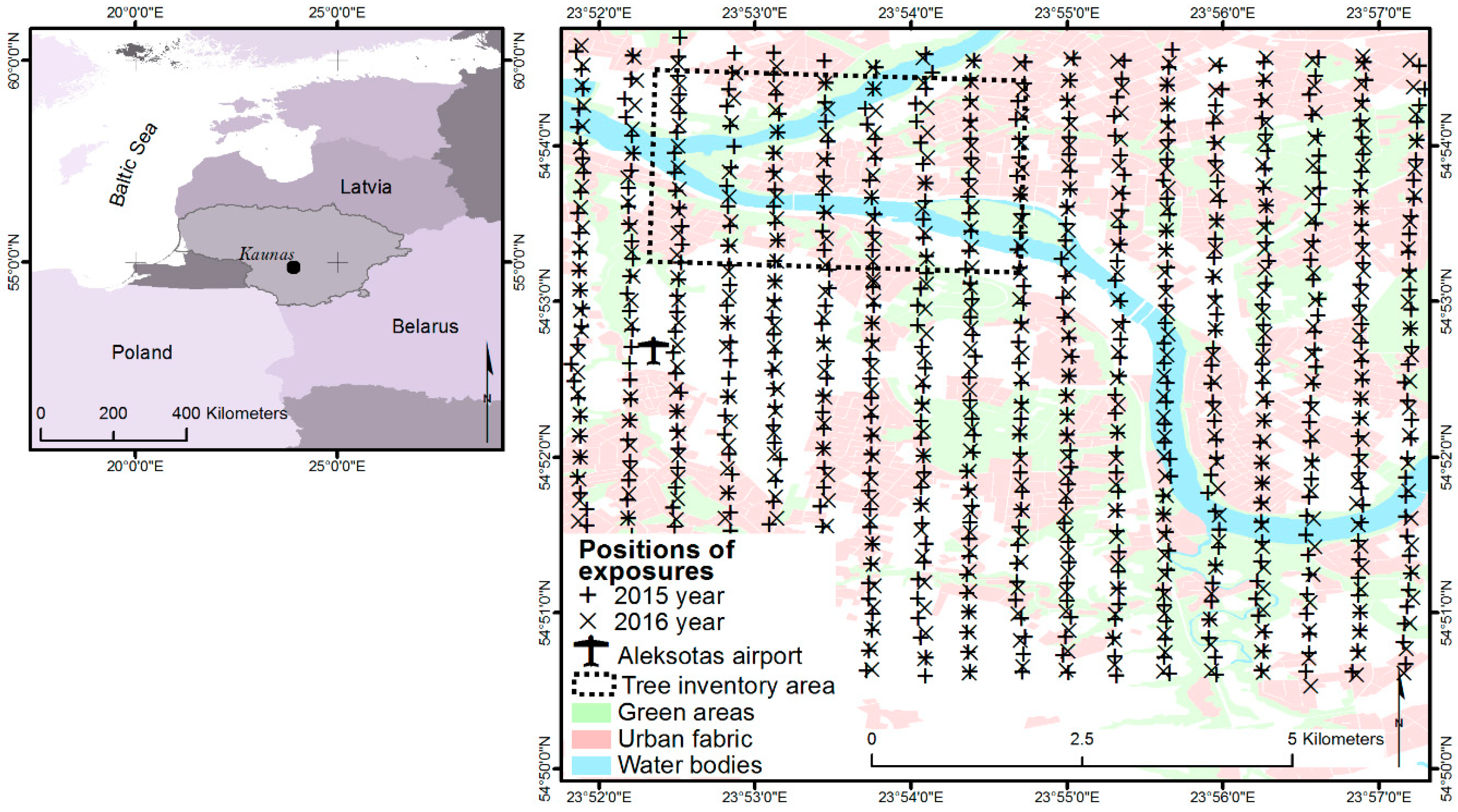
2.1. Study Area
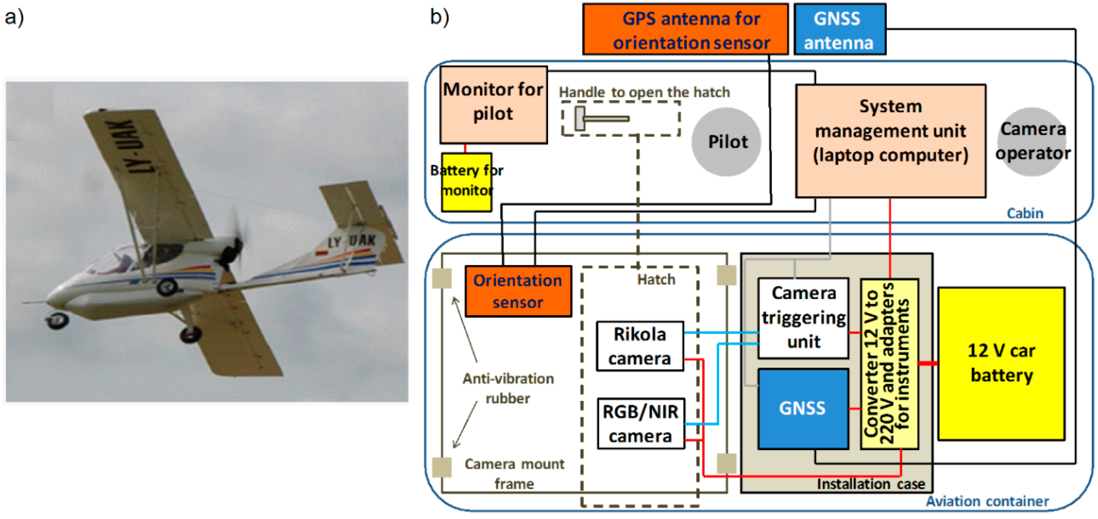
2.2. Imaging System
2.3. Imaging Missions and Image Processing
2.4. Tree Data Collection
2.5. Classification Approaches and Accuracy Assessment
- No feature selection, i.e., all extracted features were used in the classification. Hereafter, this feature selection approach is referred to as “all spectral features”.
- Spectral features were processed using a principal components (PC) analysis and transformation of the data in conjunction with a Ranker search, installed in Weka v3.8.2 software [68]. The number of PCs used in the classification was determined by choosing enough eigenvectors to account for 95% of the variance in the original data. The number of PCs used was 4 and 3 with CIR images (for the 2015 and 2016 missions, respectively), 7 and 9 with HSI, and 7 and 11 with fused CIR and HSI spectral properties. Hereafter, this feature selection approach is referred to as “principal components”.
- Correlation-based feature selection following the approach described in reference [46], which used a similar sensor in their study (hereafter, “correlation-based feature selection”). This approach is suggested for creating feature subsets correlating highly with the class value, but with low internal correlation between individual features. Weka v.3.8.2 software was used to perform the feature selection. It allows several search algorithms to be utilised to evaluate the feature subsets. We applied three different search methods, as in reference [46]:
- GeneticSearch, which is based on using the simple genetic algorithm to perform the search;
- BestFirst, which searches the space of attribute subsets by greedy hill climbing augmented with a backtracking facility; and
- GreedyStepWise, which performs a greedy forward or backward search through the space of attribute subsets.
3. Results
4. Discussion
5. Conclusions
Author Contributions
Funding
Conflicts of Interest
Appendix A
References
- Lillesand, T.M.; Kiefer, R.W.; Chipman, J.W. Remote Sensing and Image Interpretation, 6th ed.; Wiley: New York, NY, USA, 2008; 756p. [Google Scholar]
- Key, T.; Warner, T.A.; McGraw, J.B.; Fajvan, M.A. A comparison of multispectral and multitemporal information in high spatial resolution imagery for classification of individual tree species in a temperate hardwood forest. Remote Sens. Environ. 2001, 75, 100–112. [Google Scholar] [CrossRef]
- European Commission. Green Infrastructure (GI)—Enhancing Europe’s Natural Capital, Communication from the Commission to the European Parliament, the Council, the European Economic and Social Committee and the Committee of the Regions; European Commission: Brussels, Belgium, 2013. [Google Scholar]
- Melles, S.; Glenn, S.; Martin, K. Urban bird diversity and landscape complexity: Species-environment associations along a multiscale habitat gradient. Conserv. Ecol. 2003, 7, 5. [Google Scholar] [CrossRef]
- Millennium Ecosystem Assessment. Ecosystems and Human Well-Being: Synthesis; Island Press: Washington, DC, USA, 2005. [Google Scholar]
- Alvey, A.A. Promoting and preserving biodiversity in the urban forest. Urban For. Urban Green. 2006, 5, 195–201. [Google Scholar] [CrossRef]
- Nowak, D.J.; Greenfield, E.J.; Hoehn, R.E.; Lapoint, E. Carbon storage and sequestration by trees in urban and community areas of the United States. Environ. Pollut. 2013, 178, 229–236. [Google Scholar] [CrossRef] [PubMed] [Green Version]
- Pasher, M.; McGovern, M.; Khoury, M.; Duff, J. Assessing carbon storage and sequestration by Canada’s urban forests using high resolution Earth observation data. Urban For. Urban Green. 2014, 13, 484–494. [Google Scholar] [CrossRef]
- Kowarik, I. On the role of alien species in urban flora and vegetation. In Plant Invasions—General Aspects and Special Problems; Pyšek, P., Prach, K., Rejmanek, M., Wade, M., Eds.; SPB Academic Publishing: Amsterdam, The Netherlands, 1995; pp. 85–103. [Google Scholar]
- Song, I.J.; Hong, S.K.; Kim, H.O.; Byun, B.; Gin, Y. The pattern of landscapes patches and invasion of naturalized plants in developed areas of urban Seoul. Landsc. Urban Plan. 2005, 70, 205–219. [Google Scholar] [CrossRef]
- Hardin, P.J.; Jensen, R.R. The effect of urban leaf area on summertime urban surface kinetic temperatures: A Terre Haute case study. Urban For. Urban Green. 2007, 6, 63–72. [Google Scholar] [CrossRef]
- Roloff, A.; Korn, S.; Gillner, S. The climate-species-matrix to select tree species for urban habitats considering climate change. Urban For. Urban Green. 2009, 8, 295–308. [Google Scholar] [CrossRef]
- Kontogianni, A.; Tsitsoni, T.; Goudelis, G. An index based on silvicultural knowledge for tree stability assessment and improved ecological function in urban ecosystems. Ecol. Eng. 2011, 37, 914–991. [Google Scholar] [CrossRef]
- Marozas, V.; Cekstere, G.; Laivins, M.; Straigyte, L. Comparison of neophyte communities of Robinia pseudoacacia L. and Acer negundo L. in the eastern Baltic Sea region cities of Riga and Kaunas. Urban For. Urban Green. 2015, 14, 826–834. [Google Scholar] [CrossRef]
- Straigytė, L.; Cekstere, G.; Laivins, M.; Marozas, V. The spread, intensity and invasiveness of the Acer negundo in Riga and Kaunas. Dendrobiology 2015, 74, 155–166. [Google Scholar] [CrossRef]
- Garcia-Garcia, M.J.; Sánchez-Medina, A.; Alfonso-Corzo, E.; Garcia, C.G. An index to identify suitable species in urban green areas. Urban For. Urban Green. 2016, 16, 43–49. [Google Scholar] [CrossRef]
- Straigytė, L.; Vaidelys, T. Inventory of green spaces and woody plants in the urban landscape in Ariogala. South-East Eur. For. 2012, 3, 115–121. [Google Scholar] [CrossRef]
- Hostetler, A.E.; Rogan, J.; Martin, D.; DeLauer, V.; O’Neil-Dunne, J. Characterizing tree canopy loss using multi-source GIS data in Central Massachusetts, USA. Remote Sens. Lett. 2013, 4, 1137–1146. [Google Scholar] [CrossRef]
- Pu, R.; Landry, S. A comparative analysis of high spatial resolution IKONOS and WorldView-2 imagery for mapping urban tree species. Remote Sens. Environ. 2012, 124, 516–533. [Google Scholar] [CrossRef]
- McGee, J.A.; Day, S.D.; Wynne, R.H.; White, M.B. Using geospatial tools to assess the urban tree canopy: Decision support for local governments. J. For. 2012, 110, 275–286. [Google Scholar] [CrossRef]
- MacFaden, S.W.; O’Neil-Dunne, J.P.; Royar, A.R.; Lu, J.W.; Rundle, A.G. High resolution tree canopy mapping for New York City using LIDAR and object-based image analysis. J. Appl. Remote Sens. 2012, 6, 063567. [Google Scholar] [CrossRef]
- Li, X.; Shao, G. Object-based urban vegetation mapping with high-resolution aerial photography as a single data source. Int. J. Remote Sens. 2013, 34, 771–789. [Google Scholar] [CrossRef]
- Tigges, J.; Lakes, T.; Hostert, P. Urban vegetation classification: Benefits of multitemporal RapidEye satellite data. Remote Sens. Environ. 2013, 136, 66–75. [Google Scholar] [CrossRef]
- Merry, K.; Bettinger, P.; Siry, J.; Bowker, J.M. Estimating urban forest carbon sequestration potential in the Southern United States using current remote sensing imagery sources. Geogr. Tech. 2015, 10, 78–89. [Google Scholar]
- State Forest Service, Miškotvarkos Darbų Vykdymo Instrukcija (Specifications of Forest Management Planning Projects). In Lithuanian. 2010. Available online: https://www.e-tar.lt/portal/lt/legalAct/TAR.44E2BF82EF29/WIPCyylDED (accessed on 25 June 2018).
- Im, J.; Jensen, J.R. Hyperspectral remote sensing of vegetation. Geogr. Compass 2008, 2, 1943–1961. [Google Scholar] [CrossRef]
- Castro-Esau, K.L.; Sanchez-Azofeifa, G.A.; Caelli, T. Discrimination of lianas and trees with leaf-level hyperspectral data. Remote Sens. Environ. 2004, 90, 353–372. [Google Scholar] [CrossRef] [Green Version]
- Vaiphasa, C.; Ongsomwang, S.; Vaiphasa, T.; Skidmore, A.K. Tropical mangrove species discrimination using hyperspectral data: A laboratory study. Estuar. Coast. Shelf Sci. 2005, 65, 371–379. [Google Scholar] [CrossRef]
- Van Aardt, J.A.N.; Norris-Rogers, M. Spectral-age interactions in managed, even-aged Eucalyptus plantations: Application of discriminant analysis and classification and regression trees approaches to hyperspectral data. Int. J. Remote Sens. 2008, 29, 1841–1845. [Google Scholar] [CrossRef]
- Manevski, K.; Manakos, I.; Petropoulos, G.P.; Kalaitzidis, C. Discrimination of common Mediterranean plant species using field spectroradiometry. Int. J. Appl. Earth Obs. Geoinf. 2011, 13, 922–933. [Google Scholar] [CrossRef]
- Masaitis, G.; Mozgeris, G. Some peculiarities of laboratory measured hyperspectral reflectance characteristics of Scots pine and Norway spruce needles. In Proceedings of the 18th Annual International Conference Research for Rural Development, Jelgava, Latvia, 16–18 May 2012; pp. 25–32. [Google Scholar]
- Masaitis, G.; Mozgeris, G.; Augustaitis, A. Estimating crown defoliation and the chemical constituents in needles of Scots pine (Pinus sylvestris L.) trees by laboratory acquired hyperspectral data. Balt. For. 2014, 20, 314–325. [Google Scholar]
- Danusevicius, D.; Masaitis, G.; Mozgeris, G. Visible and near infrared hyperspectral imaging reveals significant differences in needle reflectance among Scots pine provenances. Silvae Genet. 2014, 63, 169–180. [Google Scholar] [CrossRef] [Green Version]
- Xiao, Q.; Ustin, S.L.; McPherson, E.G. Using AVIRIS data and multiple-masking techniques to map urban forest tree species. Int. J. Remote Sens. 2004, 25, 5637–5654. [Google Scholar] [CrossRef] [Green Version]
- Alonzo, M.; Roth, K.; Roberts, D. Identifying Santa Barbara’s urban tree species from AVIRIS imagery using canonical discriminant analysis. Remote Sens. Lett. 2013, 4, 513–521. [Google Scholar] [CrossRef]
- Alonzo, M.; Bookhagen, B.; Roberts, D.A. Urban tree species mapping using hyperspectral and lidar data fusion. Remote Sens. Environ. 2014, 148, 70–83. [Google Scholar] [CrossRef]
- Carleer, A.; Wolff, E. Exploitation of very high resolution satellite data for tree species identification. Photogramm. Eng. Remote Sens. 2004, 70, 135–140. [Google Scholar] [CrossRef]
- Cho, M.A.; Debba, P.; Mathieu, R.; Naidoo, L.; van Aardt, J.; Asner, G.P. Improving discrimination of savanna tree species through a multiple-endmember spectral angle mapper approach: Canopy-level analysis. IEEE Trans. Geosci. Remote Sens. 2010, 48, 4133–4142. [Google Scholar] [CrossRef]
- Raczko, E.; Zagajewski, B. Comparison of support vector machine, random forest and neural network classifiers for tree species classification on airborne hyperspectral APEX images. Eur. J. Remote Sens. 2017, 50, 144–154. [Google Scholar] [CrossRef]
- Ouerghemmi, W.; Gadal, S.; Mozgeris, G.; Jonikavičius, D.; Weber, C. Urban Objects Classification by Spectral Library: Feasibility and Applications. Joint Urban Remote Sensing Event (JURSE). 2017. Available online: http://0-ieeexplore-ieee-org.brum.beds.ac.uk/document/7924629/ (accessed on 7 August 2018).
- Gougeon, F.A.; Leckie, D.G. The individual tree crown approach applied to IKONOS images of a coniferous plantation area. Photogramm. Eng. Remote Sens. 2006, 72, 1287–1297. [Google Scholar] [CrossRef]
- Aksoy, S.; Gökhan, A.; Wassenaar, T. Automatic mapping of linear woody vegetation features in agricultural landscapes using very high resolution imagery. IEEE Trans. Geosci. Remote Sens. 2010, 48, 511–522. [Google Scholar] [CrossRef] [Green Version]
- Moskal, L.M.; Styers, D.M.; Halabisky, M. Monitoring urban tree cover using object-based image analysis and public domain remotely sensed data. Remote Sens. 2011, 3, 2243–2262. [Google Scholar] [CrossRef]
- Immitzer, M.; Atzberger, C.; Koukal, T. Tree species classification with RandomForest using very high spatial resolution 8-Band WorldView-2 satellite data. Remote Sens. 2012, 4, 2661–2693. [Google Scholar] [CrossRef]
- Ballanti, L.; Blesius, L.; Hines, E.; Kruse, B. Tree Species Classification Using Hyperspectral Imagery: A Comparison of Two Classifiers. Remote Sens. 2016, 8, 445. [Google Scholar] [CrossRef]
- Nevalainen, O.; Honkavaara, E.; Tuominen, S.; Viljanen, N.; Hakala, T.; Yu, X.; Hyyppä, J.; Saari, H.; Pölönen, I.; Imai, N.N.; et al. Individual tree detection and classification with UAV-based photogrammetric point clouds and hyperspectral imaging. Remote Sens. 2017, 9, 185. [Google Scholar] [CrossRef]
- Ndikumana, E.; Ho Tong Minh, D.; Baghdadi, N.; Courault, D.; Hossard, L. Deep Recurrent Neural Network for Agricultural Classification using multitemporal SAR Sentinel-1 for Camargue, France. Remote Sens. 2018, 10, 1217. [Google Scholar] [CrossRef]
- Li, W.; Fu, H.; Yu, L.; Gong, P.; Feng, D.; Li, C.; Clinton, N. Stacked Autoencoder-Based Deep Learning for Remote-Sensing Image Classification: A Case Study of African Land-Cover Mapping. Int. J. Remote Sens. 2016, 37, 5632–5646. [Google Scholar] [CrossRef]
- Maggiori, E.; Tarabalka, Y.; Charpiat, G.; Alliez, P. Convolutional Neural Networks for Large-Scale Remote Sensing Image Classification. IEEE Trans. Geosci. Remote Sens. 2017, 55, 645–657. [Google Scholar] [CrossRef]
- Forzieri, G.; Tanterib, L.; Moser, G.; Catani, F. Mapping natural and urban environments using airborne multi-sensor ADS40–MIVIS–LiDAR synergies. Int. J. Appl. Earth Obs. Geoinf. 2013, 23, 313–323. [Google Scholar] [CrossRef]
- Anderson, K.; Gaston, K.J. Lightweight unmanned aerial vehicles will revolutionize spatial ecology. Front. Ecol. Environ. 2013, 11, 138–146. [Google Scholar] [CrossRef] [Green Version]
- Colomina, I.; Molina, P. Unmanned aerial systems for photogrammetry and remote sensing: A review. ISPRS J. Photogramm. Remote Sens. 2014, 92, 79–97. [Google Scholar] [CrossRef]
- Feng, Q.; Liu, J.; Gong, J. UAV remote sensing for urban vegetation mapping using random forest and texture analysis. Remote Sens. 2015, 7, 1074–1094. [Google Scholar] [CrossRef]
- Lin, Y.; Jiang, M.; Yao, Y.; Zhang, L.; Lin, J. Use of UAV oblique imaging for the detection of individual trees inresidential environments. Urban For. Urban Green. 2015, 14, 404–412. [Google Scholar] [CrossRef]
- Honkavaara, E.; Saari, H.; Kaivosoja, J.; Pölönen, I.; Hakala, T.; Litkey, P.; Mäkynen, J.; Pesonen, L. Processing and assessment of spectrometric, stereoscopic imagery collected using a lightweight UAV spectral camera for precision agriculture. Remote Sens. 2013, 5, 5006–5039. [Google Scholar] [CrossRef] [Green Version]
- Yang, G.; Li, C.; Wang, Y.; Yuan, H.; Feng, H.; Xu, B.; Yang, X. The DOM Generation and Precise Radiometric Calibration of a UAV-Mounted Miniature Snapshot Hyperspectral Imager. Remote Sens. 2017, 9, 642. [Google Scholar] [CrossRef]
- Mozgeris, G.; Augustaitis, A. Estimating crown defoliation of Scots pine (Pinus sylvestris L.) trees using small format digital aerial images. iForest 2013, 6, 15–22. [Google Scholar] [CrossRef]
- Mozgeris, G.; Jonikavičius, D.; Jovarauskas, D.; Zinkevičius, R.; Petkevičius, S.; Steponavičius, D. Imaging from manned ultra-light and unmanned aerial vehicles for estimating properties of spring wheat. Precis. Agric. 2018. [Google Scholar] [CrossRef]
- EnsoMOSAIC Aerial Mapping System—Overview. Available online: http://mosaicmill.com/cessna_system/em_system.html (accessed on 27 July 2018).
- RIKOLA Product Family. Available online: http://senop.fi/optronics-hyperspectral (accessed on 27 July 2018).
- NOAA Solar Calculator. Available online: www.esrl.noaa.gov/gmd/grad/solcalc/ (accessed on 27 July 2018).
- Urban Atlas. Available online: https://www.eea.europa.eu/data-and-maps/data/urban-atlas (accessed on 7 August 2018).
- EnsoMOSAIC Aerial Mapping System—Components. Available online: http://mosaicmill.com/cessna_system/hardware_software.html (accessed on 27 July 2018).
- Spatial Information Portal of Lithuania. Available online: http://www.geoportal.lt/geoportal/en/web/en/home (accessed on 27 July 2018).
- Matthew, M.W.; Adler-Golden, S.M.; Berk, A.; Richtsmeier, S.C.; Levine, R.Y.; Bernstein, L.S.; Acharya, P.K.; Anderson, G.P.; Felde, G.W.; Hoke, M.P.; et al. Status of atmospheric correction using a MODTRAN4-based algorithm. SPIE Proc. 2000, 4049, 199–207. [Google Scholar] [Green Version]
- Green, A.A.; Berman, M.; Switzer, P.; Craig, M.D. A transformation for ordering multispectral data in terms of image quality with implications for noise removal. IEEE Trans. Geosci. Remote Sens. 1988, 26, 65–74. [Google Scholar] [CrossRef] [Green Version]
- Kauno Miesto Želdynų Žemėlapis. (Map of Kaunas City Green Areas). Available online: http://maps.kaunas.lt/zeldynai/ (accessed on 27 July 2018). (In Lithuanian).
- Weka 3: Data Mining Software in Java. Available online: https://www.cs.waikato.ac.nz/~ml/weka/ (accessed on 27 July 2018).
- John, G.H.; Langley, P. Estimating continuous distributions in Bayesian classifiers. In Proceedings of the Eleventh Conference on Uncertainty in Artificial Intelligence, Montreal, QC, Canada, 18–20 August 1995; Morgan Kaufmann Publishers Inc.: San Francisco, CA, USA, 1995; pp. 338–345. [Google Scholar]
- Aha, D.W.; Kibler, D.; Albert, M.K. Instance-based learning algorithms. Mach. Learn. 1991, 6, 37–66. [Google Scholar] [CrossRef] [Green Version]
- Breiman, L. Random Forest. Mach. Learn. 2001, 45, 5–32. [Google Scholar] [CrossRef]
- Class MLPClassifier. Available online: http://weka.sourceforge.net/doc.packages/multiLayerPerceptrons/weka/classifiers/functions/MLPClassifier.html (accessed on 27 July 2018).
- Quinlan, J.R. C4.5: Programs for Machine Learning; Morgan Kaufmann Publishers Inc.: San Francisco, CA, USA, 1993. [Google Scholar]
- Landis, J.R.; Koch, G. The measurement of observer agreement for categorical data. Biometrics 1977, 33, 159–174. [Google Scholar] [CrossRef] [PubMed]
- Ghiyamata, A.; Shafri, H.Z.M.; Mahdirajic, G.A.; Abdul Rashid, M.; Shariff, A.R.M.; Mansorb, S. Hyperspectral discrimination of tree species with different classifications using single- and multiple-endmember. Int. J. Appl. Earth Obs. Geoinf. 2013, 23, 177–191. [Google Scholar] [CrossRef] [Green Version]
- Baldeck, C.A.; Asner, G.P.; Martin, R.E.; Anderson, C.B.; Knapp, D.E.; Kellner, J.R.; Wright, S.J. Operational tree species mapping in a diverse tropical forest with airborne imaging spectroscopy. PLoS ONE 2015, 10, e0118403. [Google Scholar] [CrossRef] [PubMed]
- Priedītis, G.; Šmits, I.; Daģis, S.; Paura, L.; Krūmiņš, J.; Dubrovskis, D. Assessment of hyperspectral data analysis methods to classify tree species. Res. Rural Dev. 2015, 2, 7–13. [Google Scholar]
- Tagliabue, G.; Panigada, C.; Colombo, R.; Fava, F.; Cilia, C.; Baret, F.; Vreys, K.; Meuleman, K.; Rossini, M. Forest species mapping using airborne hyperspectral APEX data. Misc. Geogr. Reg. Stud. Dev. 2016, 20, 28–33. [Google Scholar] [CrossRef] [Green Version]
- Roberts, D.A.; Ustin, S.L.; Ogunjemiyo, S.; Greenberg, J.; Dobrowski, S.Z.; Chen, J.; Hinckley, T.M. Spectral and structural measures of northwest forest vegetation at leaf to landscape scales. Ecosystem 2004, 7, 545–562. [Google Scholar] [CrossRef]
- Kuusk, J.; Kuusk, A.; Lang, M.; Kallis, A. Hyperspectral reflectance of boreo-nemoral forests in a dry and normal summer. Int. J. Remote Sens. 2010, 31, 159–175. [Google Scholar] [CrossRef]
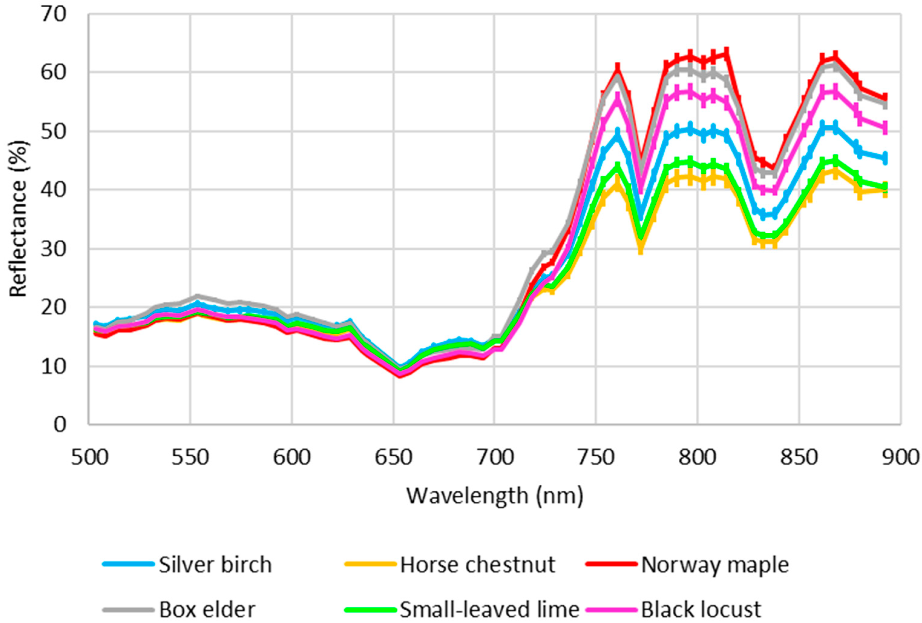
- Masaitis, G.; Mozgeris, G. The influence of the growing season on the spectral reflectance properties of forest tree species. Res. Rural Dev. 2013, 2, 20–26. [Google Scholar]
- Mozgeris, G. Miškotvarkoje naudojamų ortofototransformuotų aerovaizdų dešifravimo požymiai. [Interpretation criteria of orthophotos, used in forest inventory]. Miškininkystė 2004, 1, 49–59. (In Lithuanian) [Google Scholar]
- Lee, J.; Cai, X.; Lellmann, J.; Dalponte, M.; Malhi, Y.; Butt, N.; Morecroft, M.; Schönlieb, C.-B.; Coomes, D.A. Individual tree species classification from airborne multi-sensor imagery using robust PCA. IEEE J. Sel. Top. Appl. Earth Obs. Remote Sens. 2016, 9, 2554–2567. [Google Scholar] [CrossRef]
- Ouerghemmi, W.; Gadal, S.; Mozgeris, G.; Jonikavičius, D. Urban vegetation mapping by airborne hyperspetral imagery: Feasability and limitations. In Proceedings of the 9th Workshop on Hyperspectral Image and Signal Processing (WHISPERS), Amsterdam, The Netherlands, 23–26 September 2018. [Google Scholar]
- Kamilaris, A.; Prenafeta-Boldú, F.X. Deep learning in agriculture: A survey. Comput. Electron. Agric. 2018, 147, 70–90. [Google Scholar] [CrossRef]
- Murakami, T. Seasonal variation in classification accuracy of forest-cover types examined by a single band or band combinations. J. For. Res. 2004, 3, 211–215. [Google Scholar] [CrossRef]
- Burkholder, A. Seasonal Trends in Separability of Leaf Reflectance Spectra for Ailanthus altissima and Four Other Tree Species. Ph.D. Thesis, West Virginia University, Morgantown, WV, USA, 2010. [Google Scholar]
- Hesketh, M.; Sánchez-Azofeifa, G.A. The effect of seasonal spectral variation on species classification in the Panamanian tropical forest. Remote Sens. Environ. 2012, 118, 73–82. [Google Scholar] [CrossRef] [Green Version]
- Masaitis, G. The Potential of Hyperspectral Imaging to Detect Forest Tree Species and Evaluate Their Condition. Ph.D. Thesis, Aleksandras Stulginskis University, Akademija, Lithuania, 2013. [Google Scholar]
- Ciesla, W.M. Remote Sensing in Forest Health Protection; FHTET Report No. 00-03; Forest Health Technology Enterprise Team, USDA Forest Service, Remote Sensing Applications Center: Salt Lake City, UT, USA; Forest Health Technology Enterprise: Fort Collins, CO, USA, 2000; Available online: https://www.fs.fed.us/foresthealth/technology/pdfs/RemoteSensingForestHealth00_03.pdf (accessed on 7 August 2018).


| Mission | Setting Type | Setting Values |
|---|---|---|
| 17 July 2015 | Central wavelength, nm | 503.36; 528.29; 553.46; 578.03; 602.93; 628.42; 653.17; 677.93; 703.02; 728.01; 753.40; 778.07; 803.20; 827.90; 852.71; 877.78 |
| 17 July 2015 | Full width at half maximum, nm | 10.22; 10.34; 8.92; 9.60; 12.03; 11.24; 10.15; 10.73; 9.18; 9.00; 8.94; 8.67; 10.03; 10.06; 14.07; 13.25 |
| 11 September 2016 | Central wavelength, nm | 503.45; 508.36; 513.89; 520.07; 528.13; 532.48; 538.10; 544.37; 553.18; 556.33; 562.03; 568.38; 574.12; 578.59; 586.29; 592.09; 597.90; 602.43; 610.23; 616.11; 622.00; 628.56; 634.49; 637.80; 653.29; 657.99; 664.05; 670.11; 677.53; 682.26; 688.34; 694.42; 699.84; 703.23; 712.05; 718.16; 724.28; 728.36; 735.85; 741.99; 748.14; 753.60; 760.44; 765.92; 772.09; 778.26; 784.44; 789.94; 796.14; 803.03; 807.85; 814.06; 820.28; 827.89; 832.04; 838.28; 843.50; 852.61; 855.66; 861.76; 867.87; 878.08; 880.13; 892.44 |
| 11 September 2016 | Full width at half maximum, nm | 12.35; 12.11; 11.86; 11.61; 11.31; 11.16; 10.98; 10.80; 10.58; 10.50; 10.38; 10.25; 10.15; 10.07; 9.94; 9.86; 9.77; 9.71; 9.60; 9.52; 9.43; 9.33; 9.24; 9.18; 9.56; 9.54; 9.52; 9.49; 9.45; 9.42; 9.38; 9.34; 9.30; 9.27; 9.20; 9.15; 9.09; 9.05; 8.99; 8.93; 8.87; 8.82; 8.76; 8.72; 8.67; 8.62; 8.57; 8.53; 8.50; 8.46; 8.44; 8.41; 8.39; 8.37; 8.37; 8.37; 12.93; 12.80; 12.76; 12.68; 12.60; 12.47; 12.45; 12.30 |
| English Name | Scientific Name | Number of Crowns | |||
|---|---|---|---|---|---|
| Image Acquisition in 2015 | Image Acquisition in 2016 | ||||
| HSI | CIR | HSI | CIR | ||
| Silver birch | Betula pendula Roth | 126 | 119 | 115 | 111 |
| Horse chestnut | Aesculus hippocastanum L. | 111 | 97 | 95 | 95 |
| Norway maple | Acer platanoides L. | 150 | 135 | 135 | 137 |
| Box elder | Acer negundo L. | 107 | 103 | 80 | 79 |
| Small-leaved lime | Tilia cordata Mill. | 164 | 149 | 156 | 157 |
| Black locust | Robinia pseudoacacia L. | 109 | 95 | 87 | 87 |
| Algorithm | All Spectral Features | Correlation Based Feature Selection | Principal Components | |||
|---|---|---|---|---|---|---|
| Overall Accuracy | Kappa | Overall Accuracy | Kappa | Overall Accuracy | Kappa | |
| Mission 2015 | ||||||
| Nikon colour-infrared images | ||||||
| Naïve Bayes | 33.0 | 0.17 | 34.1 | 0.18 | 32.3 | 0.16 |
| k-NN | 31.1 | 0.17 | 28.9 | 0.14 | 23.9 | 0.10 |
| RandomForest | 38.8 | 0.25 | 34.9 | 0.21 | 30.3 | 0.15 |
| Multilayer Perceptron | 49.4 | 0.39 | 38.7 | 0.25 | 34.0 | 0.19 |
| C 4.5 | 33.1 | 0.19 | 30.0 | 0.15 | 26.9 | 0.12 |
| Rikola hyperspectral images | ||||||
| Naïve Bayes | 42.0 | 0.30 | 43.7 | 0.32 | 41.4 | 0.29 |
| k-NN | 37.0 | 0.23 | 40.2 | 0.27 | 38.0 | 0.25 |
| RandomForest | 48.5 | 0.37 | 38.4 | 0.26 | 44.6 | 0.33 |
| Multilayer Perceptron | 55.0 | 0.46 | 54.7 | 0.45 | 44.6 | 0.33 |
| C 4.5 | 38.6 | 0.26 | 38.1 | 0.25 | 37.1 | 0.24 |
| Fusing hyperspectral and colour-infrared data | ||||||
| Naïve Bayes | 42.6 | 0.31 | 43.3 | 0.31 | 44.1 | 0.32 |
| k-NN | 40.3 | 0.28 | 39.9 | 0.27 | 40.9 | 0.28 |
| RandomForest | 50.4 | 0.40 | 48.6 | 0.38 | 50.0 | 0.39 |
| Multilayer Perceptron | 57.8 | 0.49 | 55.4 | 0.46 | 44.5 | 0.33 |
| C 4.5 | 41.6 | 0.29 | 39.0 | 0.26 | 39.4 | 0.27 |
| Mission 2016 | ||||||
| Nikon colour-infrared images | ||||||
| Naïve Bayes | 34.8 | 0.20 | 37.2 | 0.22 | 35.4 | 0.18 |
| k-NN | 33.8 | 0.19 | 34.7 | 0.20 | 26.6 | 0.11 |
| RandomForest | 43.2 | 0.30 | 38.7 | 0.25 | 32.1 | 0.16 |
| Multilayer Perceptron | 51.7 | 0.41 | 46.8 | 0.35 | 35.6 | 0.18 |
| C 4.5 | 34.2 | 0.20 | 31.4 | 0.16 | 28.5 | 0.12 |
| Rikola hyperspectral images | ||||||
| Naïve Bayes | 43.1 | 0.31 | 42.4 | 0.30 | 48.6 | 0.37 |
| k-NN | 42.6 | 0.30 | 38.8 | 0.29 | 42.6 | 0.30 |
| RandomForest | 50.4 | 0.39 | 48.6 | 0.37 | 50.4 | 0.39 |
| Multilayer Perceptron | 62.6 | 0.54 | 58.7 | 0.50 | 47.5 | 0.36 |
| C 4.5 | 39.1 | 0.26 | 35.6 | 0.22 | 40.0 | 0.27 |
| Fusing hyperspectral and colour-infrared data | ||||||
| Naïve Bayes | 43.4 | 0.32 | 44.5 | 0.33 | 50.1 | 0.39 |
| k-NN | 40.6 | 0.28 | 40.9 | 0.28 | 46.0 | 0.34 |
| RandomForest | 49.3 | 0.37 | 47.3 | 0.35 | 50.1 | 0.39 |
| Multilayer Perceptron | 62.5 | 0.54 | 62.1 | 0.54 | 50.0 | 0.39 |
| C 4.5 | 37.3 | 0.24 | 38.3 | 0.25 | 39.0 | 0.26 |
| Compared Cases | Feature Selection | Algorithm | ||||
|---|---|---|---|---|---|---|
| Naïve Bayes | k-NN | Random Forest | Multilayer Perceptron | C 4.5 | ||
| CIR 2015 vs. HSI 2015 | All spectral features | 2.88 | 1.57 | 2.56 | 1.45 | 1.52 |
| CIR 2016 vs. HSI 2016 | All spectral features | 2.60 | 2.22 | 1.04 | 2.84 | 3.20 |
| CIR 2015 vs. HSI 2015 | Correlation-based feature selection | 3.16 | 2.49 | 1.06 | 4.40 | 2.37 |
| CIR 2016 vs. HSI 2016 | Correlation-based feature selection | 1.82 | 1.24 | 2.55 | 3.15 | 1.21 |
| CIR 2015 vs. HSI 2015 | Principal components | 2.90 | 4.15 | 3.95 | 3.13 | 2.99 |
| CIR 2016 vs. HSI 2016 | Principal components | 3.99 | 4.54 | 5.05 | 3.74 | 3.39 |
| Fused CIR/HSI 2015 vs. HSI 2015 | All spectral features | 0.16 | 0.92 | 3.02 | 0.74 | 0.83 |
| Fused CIR/HSI 2016 vs. HSI 2016 | All spectral features | 0.10 | 0.28 | 0.56 | 0.02 | 0.48 |
| Fused CIR/HSI 2015 vs. HSI 2015 | Correlation-based feature selection | 0.11 | 0.10 | 2.63 | 0.13 | 0.27 |
| Fused CIR/HSI 2016 vs. HSI 2016 | Correlation-based feature selection | 0.55 | 1.58 | 0.31 | 0.90 | 0.80 |
| Fused CIR/HSI 2015 vs. HSI 2015 | Principal components | 0.49 | 0.79 | 1.45 | 0.01 | 0.63 |
| Fused CIR/HSI 2016 vs. HSI 2016 | Principal components | 0.39 | 0.92 | 0.13 | 0.68 | 0.26 |
| HSI 2015 vs. HSI 2016 | All spectral features | 0.26 | 0.64 | 0.50 | 1.88 | 0.19 |
| HSI 2015 vs. HSI 2016 | Correlation-based feature selection | 0.30 | 0.11 | 2.40 | 0.94 | 0.81 |
| HSI 2015 vs. HSI 2016 | Principal components | 1.76 | 1.94 | 1.43 | 0.66 | 0.64 |
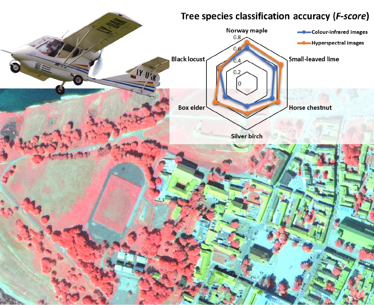
| Type of Images | Mission | F-Score by Tree Species | ||||||
|---|---|---|---|---|---|---|---|---|
| Norway Maple | Small-Leaved Lime | Horse Chestnut | Silver Birch | Box Elder | Black Locust | Average | ||
| Nikon colour-infrared images | 2015 | 0.615 | 0.552 | 0.436 | 0.453 | 0.340 | 0.468 | 0.478 |
| 2016 | 0.621 | 0.542 | 0.497 | 0.379 | 0.433 | 0.544 | 0.614 | |
| Rikola hyperspectral images | 2015 | 0.617 | 0.571 | 0.502 | 0.505 | 0.561 | 0.509 | 0.544 |
| 2016 | 0.716 | 0.674 | 0.617 | 0.511 | 0.633 | 0.633 | 0.532 | |
| Fused hyperspectral and colour-infrared data | 2015 | 0.644 | 0.592 | 0.534 | 0.517 | 0.635 | 0.511 | 0.572 |
| 2016 | 0.724 | 0.703 | 0.610 | 0.487 | 0.539 | 0.591 | 0.609 | |
© 2018 by the authors. Licensee MDPI, Basel, Switzerland. This article is an open access article distributed under the terms and conditions of the Creative Commons Attribution (CC BY) license (http://creativecommons.org/licenses/by/4.0/).
Share and Cite
Mozgeris, G.; Juodkienė, V.; Jonikavičius, D.; Straigytė, L.; Gadal, S.; Ouerghemmi, W. Ultra-Light Aircraft-Based Hyperspectral and Colour-Infrared Imaging to Identify Deciduous Tree Species in an Urban Environment. Remote Sens. 2018, 10, 1668. https://0-doi-org.brum.beds.ac.uk/10.3390/rs10101668
Mozgeris G, Juodkienė V, Jonikavičius D, Straigytė L, Gadal S, Ouerghemmi W. Ultra-Light Aircraft-Based Hyperspectral and Colour-Infrared Imaging to Identify Deciduous Tree Species in an Urban Environment. Remote Sensing. 2018; 10(10):1668. https://0-doi-org.brum.beds.ac.uk/10.3390/rs10101668
Chicago/Turabian StyleMozgeris, Gintautas, Vytautė Juodkienė, Donatas Jonikavičius, Lina Straigytė, Sébastien Gadal, and Walid Ouerghemmi. 2018. "Ultra-Light Aircraft-Based Hyperspectral and Colour-Infrared Imaging to Identify Deciduous Tree Species in an Urban Environment" Remote Sensing 10, no. 10: 1668. https://0-doi-org.brum.beds.ac.uk/10.3390/rs10101668