Article

The Global Mangrove Watch—A New 2010 Global Baseline of Mangrove Extent

1
Department of Geography and Earth Sciences, Aberystwyth University, Aberystwyth SY23 3DB, UK
2
Solo Earth Observation (soloEO), Tokyo 104-0054, Japan
3
School of Biological, Earth and Environmental Sciences (BEES), University of New South Wales (UNSW), High Street, Kensington, NSW 2052, Australia
4
International Water Management Institute, Regional Office for SE Asia and The Mekong, P.O. Box 4199, Vientiane
5
Wetlands International, 6700AL Wageningen, The Netherlands
6
Earth System Science Interdicsiplinary Center, University of Maryland/NASA Goddard Space Flight Center, College Park, MD 20742, USA
7
Remote Sensing Technology Center of Japan (RESTEC), Tsukuba Office, Ibaraki 305-8505, Japan
8
School of Science and Engineering, Tokyo Denki University, Saitama 350-0394, Japan
9
Institute for Land, Water and Society, Charles Sturt University, Albury, NSW 2640, Australia
*
Author to whom correspondence should be addressed.
Remote Sens. 2018, 10(10), 1669; https://0-doi-org.brum.beds.ac.uk/10.3390/rs10101669
Submission received: 31 July 2018 / Revised: 14 September 2018 / Accepted: 18 October 2018 / Published: 22 October 2018

Abstract

:
This study presents a new global baseline of mangrove extent for 2010 and has been released as the first output of the Global Mangrove Watch (GMW) initiative. This is the first study to apply a globally consistent and automated method for mapping mangroves, identifying a global extent of 137,600 km 2 . The overall accuracy for mangrove extent was 94.0% with a 99% likelihood that the true value is between 93.6–94.5%, using 53,878 accuracy points across 20 sites distributed globally. Using the geographic regions of the Ramsar Convention on Wetlands, Asia has the highest proportion of mangroves with 38.7% of the global total, while Latin America and the Caribbean have 20.3%, Africa has 20.0%, Oceania has 11.9%, North America has 8.4% and the European Overseas Territories have 0.7%. The methodology developed is primarily based on the classification of ALOS PALSAR and Landsat sensor data, where a habitat mask was first generated, within which the classification of mangrove was undertaken using the Extremely Randomized Trees classifier. This new globally consistent baseline will also form the basis of a mangrove monitoring system using JAXA JERS-1 SAR, ALOS PALSAR and ALOS-2 PALSAR-2 radar data to assess mangrove change from 1996 to the present. However, when using the product, users should note that a minimum mapping unit of 1 ha is recommended and that the error increases in regions of disturbance and where narrow strips or smaller fragmented areas of mangroves are present. Artefacts due to cloud cover and the Landsat-7 SLC-off error are also present in some areas, particularly regions of West Africa due to the lack of Landsat-5 data and persistence cloud cover. In the future, consideration will be given to the production of a new global baseline based on 10 m Sentinel-2 composites.

Graphical Abstract

1. Introduction

Mangroves are forested wetlands that are uniquely adapted to the intertidal zone. Found in the coastal zones of more than 118 countries in the tropics, subtropics and temperate regions [1,2,3], mangroves have (for centuries) provided natural resources to local populations, including food (particularly fish and invertebrates) and timber. However, through processes such as population increases, industrialisation, urban expansion and globalisation, their extent has been reduced [4] and many have been fragmented or degraded [5], particularly in Southeast Asia, where about one third (32%) of the world’s mangroves are located [6]. Many of the mangrove areas that have remained relatively intact are those that are remote, inaccessible, protected within conservation reserves or receive national protection, for example in Australia. Globally, mangroves are being increasingly affected by climatic fluctuations, including those induced by human activities [5]. At the same time, mangroves are receiving greater recognition for their role in food provision, coastal protection (e.g., from large storms), reserves of biodiversity [7] and as a large carbon store [8]. Hence, there are numerous and increasing efforts to ensure protection and restoration across their range. A fundamental requirement for mangrove protection and restoration is information about current and historical mangrove distributions and conditions. While critical for informing efforts that support conservation, sustainable management, and restoration of these ecosystems, data on mangrove status and extent are necessary to meet reporting requirements for signatories to the Ramsar Convention on Wetlands and other countries with mangroves in their territories who are striving to meet the Sustainable Development Goals [5,9].
At a global level, maps of mangrove extent have previously been generated by Spalding et al. for 1960–1996 [3] and 1999–2003 [2], by curating the best available national and regional maps, and by the United States Geological Survey (USGS; [1]) for 2000, based on the classification of Landsat sensor data primarily from 1997–2000. The FAO [4,10,11] have also conducted surveys to estimate global extent for 1980, 1990 and 2000 and, in the later studies, both the FAO and Spalding et al. [2] referred to the 2000 Giri et al. [1] to fill in gaps in coverage. The map of Giri et al. [1] has been regarded as the most globally consistent because of the standardised use of Landsat sensor data and methodology within a defined period but, in some cases, the contribution of local to regionally-derived maps to Spalding et al. [2] results in better mapping (depending on the scales and methods used). Hence, whilst the maps of mangrove area are broadly in agreement, many differences exist in terms of area and boundary locations with these sometimes exaggerated by differences in accuracy in the geometric location, scale and generalisation of the map products. The maps generated are also historical (currently by at least two decades) and are unable to be easily updated and certainly not on a regular (e.g., annual) basis. Rates of mangrove loss can also then not be determined as the products from different years are based on different methods.
To address the need for timely information on mangroves at a global level, the Japan Aerospace Exploration Agency (JAXA) Kyoto & Carbon (K&C) Initiative formulated the Global Mangrove Watch (GMW), which aimed to produce consistent 25 m spatial resolution maps of mangrove extent across their range by generating a baseline map for 2010. For mapping, Japanese L-band Synthetic Aperture Radar (SAR) data were considered most appropriate given their global coverage and sensitivity to the woody components of mangroves [12]. However, a limitation is that mangroves are often difficult to distinguish from other land covers (particularly forests and plantations) on the landward margins. For this reason, Landsat sensor data were integrated into the analysis to improve the baseline map. The mapping was also confined to locations with conditions considered suitable to support mangroves. The objective of the GMW is to provide the information needed by a wide range of users, including wetland and forest managers, civil society organisations, contracting partners of the Ramsar Convention, and countries with mangroves in their territories.
Many studies have used Earth Observation (EO) data to map mangrove extent. At a global level, the study of Giri et al. [1] was the first, with this using an unsupervised classification approach and manual selection of classes associated with mangroves. Many studies have used the Giri et al. [1] product as a basis for further analysis. For example, Hamilton and Casey [13] intersected the Giri et al. [1] map with the forest cover change of Hansen et al. [14] to assess changes in mangrove extent. Thomas et al. [6] was the first to consider L-band SAR for global assessment of mangrove change, which was assessed visually by on a 1 × 1 grid overlain onto a composite of Japanese Earth Resources Satellite (JERS-1) SAR from 1996 and Advanced Land Observing Satellite (ALOS PALSAR) data from 2007 and 2010. Causes of change were also reviewed based on features including shape and context. Other studies have been more focused on local sites, such as a single delta (e.g., the Mangoky River delta, Madagascar [15], Mekong Delta, Vietnam [16]) or countries (e.g., Mozambique [17], Philippines’ [18], Kenya [19], and Mexico [20]). Methods adopted have varied. The majority have used optical (primarily Landsat) datasets (e.g., [15,17,18,19]), while a few have fused optical and SAR data (e.g., [21,22]). In terms of analysis, a broad range of techniques have been used, including object orientated methods making use of image segmentation (e.g., [23]), rule based classifiers (e.g., [21]), unsupervised classifiers (e.g., [17,18,24]) and machine learning methods (e.g., [22,23]). While there is no clear dominant direction in terms of methodology for assessing mangrove extent, a significant gap is the lack of studies that have sought to develop and apply a single consistent methodology that is repeatable over large geographic areas, including at the global level. Therefore, this study aims to provide a new updated baseline of global mangrove extent, which can be used as a basis for studying mangrove change and uses a single globally consistent methodology.

2. Methods

The new global mangrove baseline has been generated using a combination of Synthetic Aperture Radar (SAR) from the Advanced Land Observing Satellite (ALOS) Phased-Array L-band Synthetic Aperture Radar (PALSAR) and optical satellite data from Landsat-5 Thematic Mapper (TM) and Landsat-7 Enhanced TM (ETM+). The overall approach followed four stages: (a) extraction of a coastal water mask from the PALSAR data; (b) generation of a mangrove “habitat” layer that identified areas that were actually or potentially able to support mangroves; (c) generation of an initial baseline classification using the PALSAR data only; and (d) refinement of the initial baseline classification using Landsat sensor composites to improve the distinction of the landward border between mangroves and other terrestrial land covers. A final quality assurance (QA) of the resulting baseline product was then undertaken through visual assessment and, where appropriate, errors were corrected. An overview of the methods for producing the new mangrove baseline is shown in Figure 1.
Unless otherwise stated, all data processing was undertaken using the open source Remote Sensing and GIS Software Library (RSGISLib [25]), the KEA file format [26], the Scikit-Learn [27] machine learning library and scripted in python as outlined by Clewley et al. [28].

2.1. Datasets

Using data acquired in 2010, a baseline map of mangrove extent was generated by integrating ALOS PALSAR and a composite of Landsat sensor data and referencing the 2000 Shuttle Radar Topographic Mission (SRTM) 30 m Digital Elevation Model data and existing products delineating shorelines, surface water occurrence and previous attempts to delineate global mangrove extents. These datasets are summarised in Table 1
From the global shoreline dataset, a global ocean regions dataset was derived to identify oceanic water bodies. The shoreline dataset was rasterised onto the same pixel grid as the ALOS PALSAR data and oceanic water was defined as pixels that were 200 pixels (∼5000 m) from the defined shoreline.
All data were re-sampled or rasterised onto the same 0.8 arc-second pixel grid as the ALOS PALSAR data. For the SRTM data cubic spline interpolation was used, while for other continuous data (e.g., Landsat) a cubic convolution was applied and for categorical data nearest neighbour interpolation was used.

2.1.1. ALOS PALSAR

The ALOS PALSAR dual polarisation (HH+HV) backscatter data used were provided by JAXA as 1 × 1 mosaic tiles. The nominal spatial resolution was 25 m (0.8 arc seconds) and data were provided in the WGS84 (EPSG:4326) coordinate system. The mosaics are openly available in the public domain (http://www.eorc.jaxa.jp/ALOS/en/palsarfnf/fnfindex.htm). The processing undertaken to produce the tiled mosaics is detailed in Shimada et al. [33]. Global mosaics from JERS-1 SAR, ALOS PALSAR and ALOS-2 PALSAR-2 were available for 1996, annually from 2007 to 2010 and from 2015 to 2017. However, the 2010 mosaic was the most complete in terms of temporal consistency and spatial coverage and therefore was defined as the baseline (reference) year.

2.1.2. Landsat Composites

Although the ALOS PALSAR dual polarisation L-band SAR data provided a reasonable level of discrimination of mangroves from other land cover types (particularly bare ground), there was some confusion with other wetland or forest types. This was particularly the case for certain types of adjoining terrestrial forests and wetlands with similar structure to mangroves. However, mangroves were distinct from many of these land covers within the Landsat sensor data, particularly in the near infrared and shortwave infrared wavelength regions. For this reason, composite images were generated using Landsat sensor data acquired for 2010, although 2009 and 2011 images were also used, where necessary, to provide sufficient imagery for the processing. In order to minimise the impact of the Landsat 7 scan-line (SLC-off) error, which results in no-data striping in the imagery, Landsat 5 data were primarily selected when available. To identify the scenes to download for each Landsat row/path, the following sequence of rules were applied:
  • Identify 10 Landsat 5 scenes with less than 10% cloud cover from 2010.
  • If less than 10 scenes available, then add Landsat 7 scenes with less than 10% cloud cover from 2010.
  • If less than 5 scenes, then add Landsat 5 and 7 scenes from 2010 with less than 50% cloud up to a maximum of 15 scenes.
  • If less than 5 scenes, then extend time range to 2009–2011 and repeat Steps 1–3.
A total of 15,346 top-of-atmosphere Landsat scenes from 1766 row/paths were downloaded using the Google Cloud API (https://cloud.google.com/storage/docs/public-datasets/landsat). The images where processed to surface reflectance, cloud masked and topographically corrected using the “Atmospheric and Radiometric Correction of Satellite Imagery” (ARCSI [34]) software. ARCSI derives a scene based aerosol optical depth (AOD) value using a dark object subtraction (DOS [35]) where a numerical inversion of the 6S [36] atmospheric model is applied to derive an AOD value based on the Blue wavelength. The 30 m (1 arc-second) SRTM elevation model was used to construct a look-up table (LUT) for correction with respect to elevation, which was applied subsequently to the input image to derive standardised (i.e., topographically corrected) reflectance using the approach of Shepherd and Dymond [37]. The FMASK [38,39] cloud masking algorithm was applied for removal of cloud and cloud shadow.
To allow fusion with the ALOS PALSAR data, the resulting Landsat data were re-sampled, using cubic convolution, to match the 0.8 arc-second pixel grid of the ALOS PALSAR data. A maximum NDVI compositing [40,41] processing chain was then applied using RSGISLib [25] at a project level (see Section 2.2) to generate a single Landsat composite image corresponding with the project region defined using the ALOS PALSAR data.

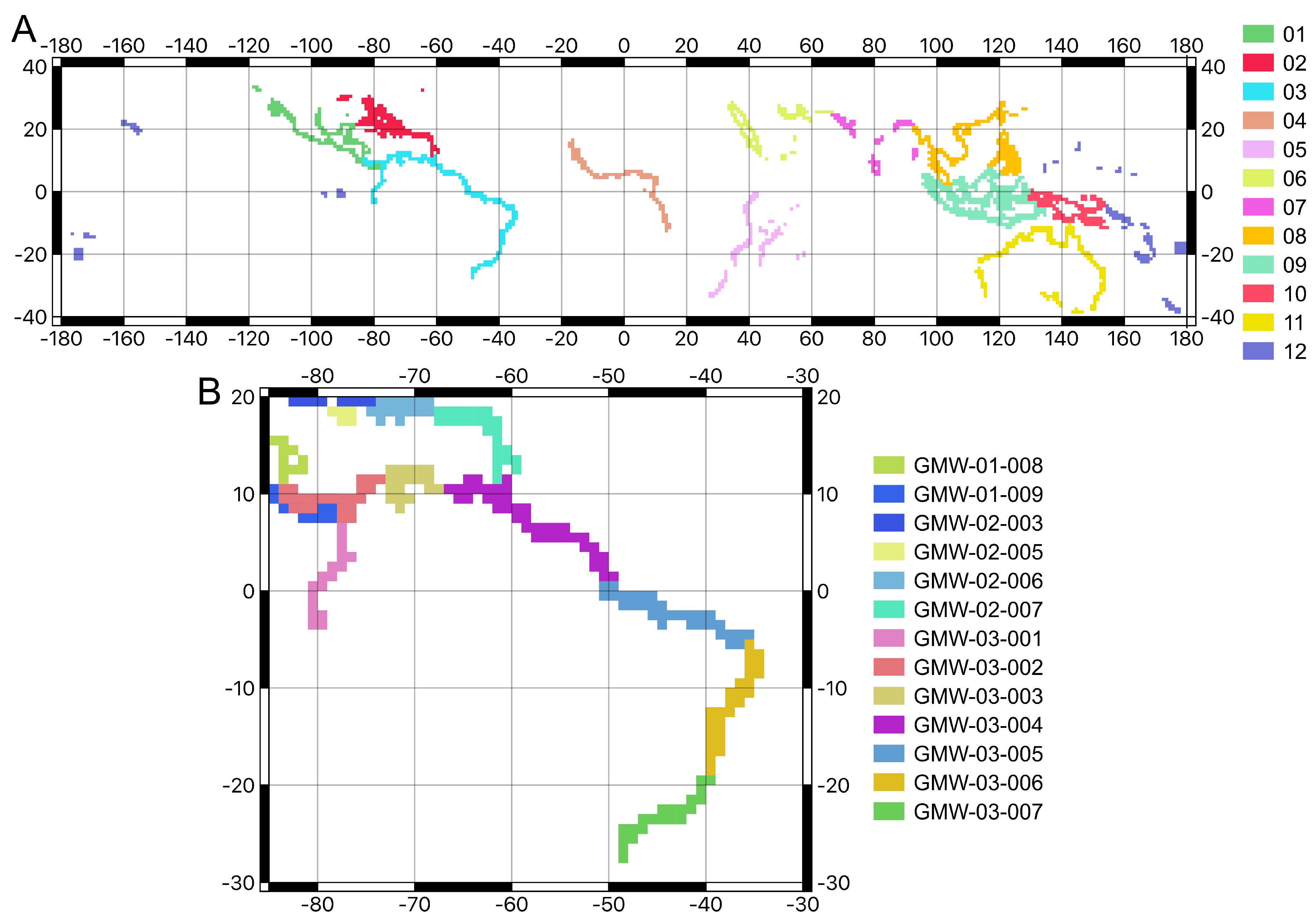
2.2. Project Region Definition

To undertake the processing, 128 project regions were defined that grouped the 1 × 1 tiles such that: (a) no continuous area of mangroves was split by a project border; (b) the mangroves within a project were considered to be contained within a similar bio-geographic region and (c) the computational requirements of processing the projects were appropriate (i.e., balancing speed of processing with available computing resource).
The projects were defined by the union of Giri et al. [1] and Spalding et al. [2] datasets, where each were buffered by 0.1 and touching or overlapping polygons merged. The resulting polygons where clustered using the approach outlined in Bunting et al. [42] where the minimum spanning tree was created and edges with a length >0.5 or greater than 1 standard deviation of the edge lengths in the tree removed creating individual clusters. The resulting groups where then assessed, with small regions merged into larger regions and large regions split when these were deemed too large for efficient computational processing. This resulted in 131 project regions globally, although, for three, there were no ALOS PALSAR data and so they were excluded. The resulting 128 projects where intersected with the 1 × 1 tile grid and grouped into 12 geographic regions (Figure 2) to create a hierarchical numbering system.

2.3. Coastal Mask

Mangroves are found within a coastal environment and therefore a key component of defining the mangrove habitat mask was to define a coastal water mask. To achieve this, a water mask was defined using a per-pixel Extremely Randomized Trees classification using Scikit-Learn [27] and RSGISLib [25] software. The number of estimators for the Extremely Randomized Trees classifier was defined as 500 following a grid search sensitivity analysis. The classification was performed using the ALOS PALSAR HH and HV polarisations, the ratio of HH/HV, local incident angle and acquisition date.
The key step in defining the coastal water mask was to define the training samples and regions to be classified, which was performed automatically. An initial water mask was produced using a threshold of >20 water occurrences, and this was subsequently intersected with the oceanic region (Section 2.1) to identify oceanic water. A coastal region was then defined as the area 20 pixels (∼500 m) either side of the shoreline with a bathymetry depth of > 100 m. Additional regions based on 80 pixels (∼2000 m) either side of the shoreline and a water occurrence <80 were added to this mask, with this then defining the region to be classified. 100,000 training pixels were then extracted randomly for land and water from regions between >20 (∼500 m) and <80 (∼2000 m) pixels away from the shoreline, with this defined as water or land using the water mask retrieved from the water occurrence layer.
Following the classification, a refinement was performed to remove small features, which required clumping the classification to identify connected regions of a single class. Clumps classified as land with an area of <20 pixels (∼12,500 m 2 ) and >20 water occurrence observations were assigned to the water class, while water regions with an area of <50 pixels (∼31,250 m 2 ) were assigned to land. These thresholds were identified through a sensitivity analysis and by visually assessing the resulting maps.
The thresholds used for generating the coastal mask were identified through an iterative sensitivity analysis based on a visual inspection of the resulting maps for a number of projects and sites globally representing a range of mangrove habitats.

2.4. Mangrove Habitat

Mangroves exist within a specific ecological niche, which can be used to eliminate much of the area where they will not be found. To define the region to be classified, and from which the non-mangrove pixels were selected, the following rules were defined, applied on a per-project basis. First, the SRTM elevation needed to be less than 110% of the 99th percentile of the elevation of mangrove pixels. If the resulting threshold was less than 5 m the threshold was set to 30 m, remembering that the SRTM is a surface model and therefore includes a component of vegetation height. The second rule, defined that the distance from the coastal water mask needed to be less than 110% of the 99th percentile of the distance of the mangrove pixels.
Within the region defined above, a classification was subsequently performed. In total, 100,000 mangrove training pixels were randomly extracted from a union of the existing global mangrove maps from Giri et al. [1] and Spalding et al. [2], while 100,000 non-mangrove training samples were randomly extracted from within the region but outside of the mangrove union. If less than 100,000 mangrove pixels were available, then the number of samples selected for both classes was equal to the number of mangrove pixels within the project.
The classification was performed using the Extremely Randomized Trees classifier, with 100 estimators, defined through the use of a grid search sensitivity analysis of classifier parameters. The input variables to the classification were: (a) pixel longitude and latitude; (b) distance to water (defined using the coastal mask); (c) surface elevation defined by the SRTM; (d) distance to the oceanic layer; and (e) distances to the mangrove extents of Giri et al. [1] and Spalding et al. [2]. The resulting habitat mask was visually checked and missing regions, including those that were not identified in the Giri et al. [1] and Spalding et al. [2] products, were added manually.
The mangrove habitat layer (to be available at http://www.globalmangrovewatch.org) defines the maximum possible extent of mangrove habitat and therefore would not be needed to re-calculated for any subsequent mangrove mapping efforts.

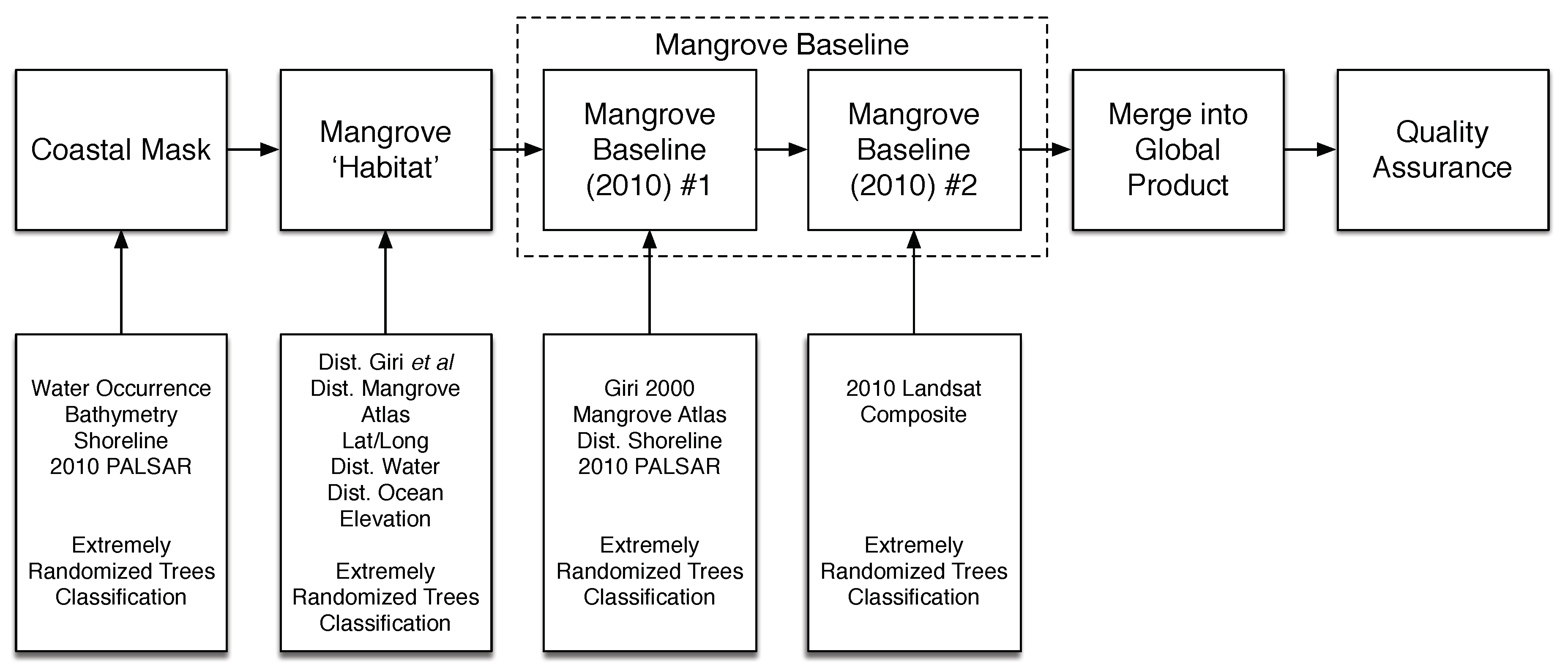
2.5. Baseline Classification

The new baseline was classified in two independent steps: first using the ALOS PALSAR and then the Landsat data. The ALOS PALSAR data were geographically contained entirely within the projects, which allowed complete classification, but there were occasional gaps in the coverage of the Landsat sensor data primarily because of cloud cover. In these gaps, the classification was based solely on the ALOS PALSAR data.

2.5.1. Classification: ALOS PALSAR

The classification was undertaken using the Extremely Randomized Trees classifier, based on 100 estimators that were also defined through a grid search sensitivity analysis. The input variables were ALOS PALSAR HH and HV data (transformed to log unit dB), the ratio of HH/HV, pixel longitude and latitude and the mangrove probability. Mangrove probability was defined using the union of mangrove extent and generating a multi-dimensional histogram for the HH, HV and HH/HV data for mangroves (defined using Giri et al. [1]) with a bin width of 0.25. The histogram was converted to a probability distribution function, which was used to calculate a probability of mangroves occurring in each pixel.
Training samples where defined through random sampling where 100,000 mangrove and non-mangrove samples were taken, resulting in 200,000 in total per project. For mangrove, 20,000 samples were extracted from the intersection of the Giri et al. [1] and Spalding et al. [2] products and the remaining 80,000 were taken from the union of the two products. The non-mangrove samples were also split, with 20,000 from within the habitat mask and 80,000 outside. The region outside the habitat mask, within which training samples were selected, was defined as <150 pixels (∼3750 m) from the union of the mangrove products over areas of water and <250 pixels (∼6250 m) over terrestrial areas. The training points were visually checked and edited with reference to Google Earth Imagery as well as the ALOS PALSAR and Landsat sensor imagery. In total, 20 M training points were defined globally across the 128 projects.

2.5.2. Classification: Landsat

Using only a classification of ALOS PALSAR data, a consistent over-classification of the area of mangroves was observed with this attributed to similarities in the structure and moisture content of wetlands and forest cover types (indicated earlier). Therefore, a further refinement using optical imagery was deemed necessary. The second classification iteration used the same training samples as the ALOS PALSAR classification but samples without valid Landsat sensor data were removed. Using the Blue, Green, Red, Near-Infrared (NIR), Shortwave Infrared 1 (SWIR1) and SWIR2 spectral bands, the Extremely Randomized Trees classifier, again using 100 estimators identified through a sensitivity analysis, was applied to generate the final classification.

2.6. Merging into a Global Product

The resulting project based analysis was compiled into a single global product for 2010 on a 1 × 1 tile basis. A few project regions shared individual tiles and these needed to be merged, which was undertaken using a union operation.

2.7. Quality Assurance

Following the automated analysis, an extensive quality assurance (QA) process was undertaken. During this process, the product was visually checked against the ALOS PALSAR and Landsat sensor data as well as contemporary (2010) Google Earth imagery. Where significant errors of omission and commission were identified, polygons were drawn and edits applied.

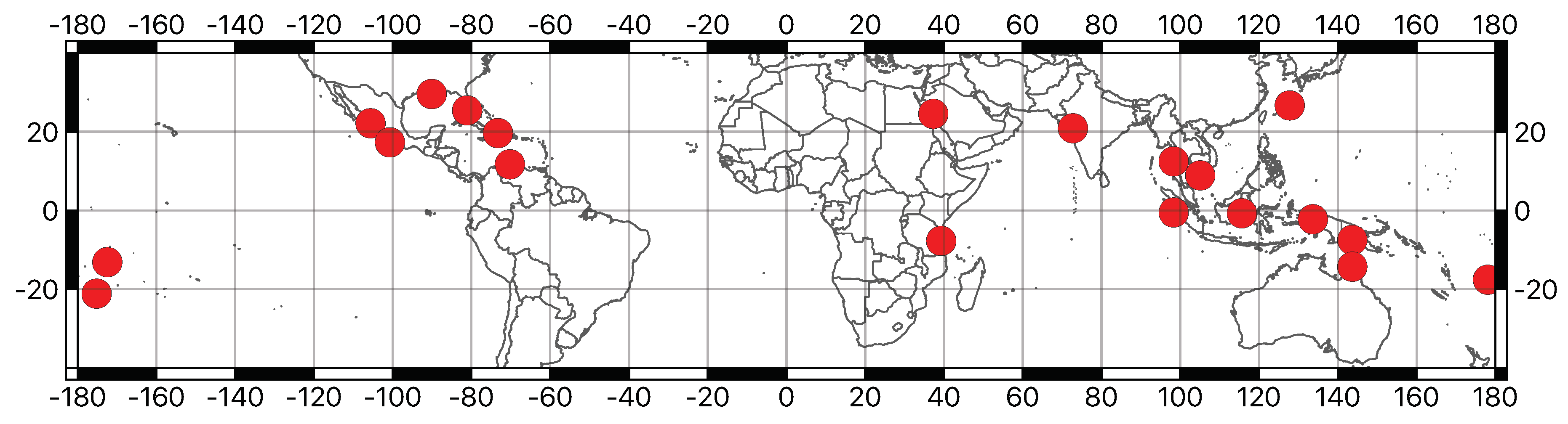
2.8. Accuracy Assessment

To assess the overall accuracy of the product, a point-based accuracy assessment was undertaken. For the accuracy assessment, a stratified random sample was undertaken within each project using the water, mangrove and terrestrial non-mangrove classes, within a 50 pixels (∼1250 m) buffer from the mangrove regions and within the mangrove habitat region. The number of accuracy samples, for each class, was 0.5% of the number of mangrove pixels, unless the resulting number of samples was less than 1000 in which case a 1% sample was taken.
Within the projects, sites were selected (Figure 3 and Table 2) based on available local knowledge and in some cases high resolution data. The accuracy assessment was undertaken using a custom QGIS plugin that guides the operator to each point, providing a simple interface to decide between classes. The imagery used for reference included high resolution Google Earth imagery, custom high resolution imagery, GMW Landsat image composites and ALOS PALSAR 2010 data.

3. Results

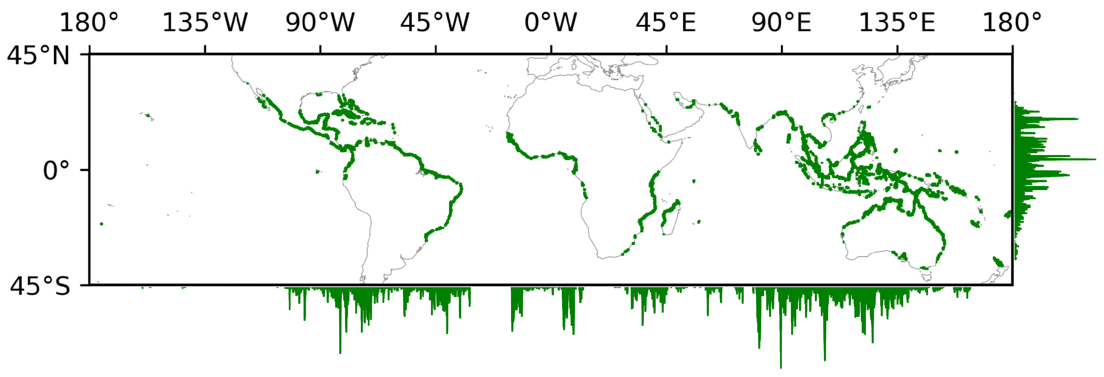
3.1. Mangrove Baseline

The resulting baseline map of global mangrove extent gives an estimated total mangrove area in 2010 of 137,600 km 2 . A Mollweide Equal Area projection was used for all area calculations. Figure 4 illustrates the global distribution of mangroves, which can be found as far north as 32.3 N (Bermuda) and as far south as 38.9 S (Australia). Figure 5 illustrates the spatial detail within the map. Approximately 96% are found between the Tropic of Cancer ( 23.4 N) and Tropic of Capricorn ( 23.4 S). Asia is estimated to account for 38.7% of the world’s mangroves, with Southeast Asia alone representing almost a third (32.2%). The Americas are estimated to comprise 28.7%, and Africa and Oceania 20.0% and 11.9%, respectively. European Overseas Territories account for 0.7%.
Table 3 shows the extent of mangroves for the six Ramsar regions. Asia is the region with the largest area of mangroves (53,278 km 2 ) with Latin America and the Caribbean (previously referred to as the Neotropics) (27,940 km 2 ) and Africa (27,465 km 2 ) regions having similar amounts. In terms of individual countries (Table 4), Indonesia contains 19.5% of the worlds mangroves and the next three highest, by area, Brazil, Australia and Mexico combined contain 22.3%.

3.2. Accuracy Assessment

The overall accuracy (Table 5) of the classification was 95.3%, with a 99% likelihood that the confidence interval, using the Wilson score interval [43], was 4.5–5.0%. Therefore, the overall accuracy was in the range 95.0–95.5%. In total, 53,878 sample points (Table 2) were used for the accuracy assessment, where the points were manually allocated to the classes of mangroves, water and terrestrial (other). In terms of mangroves, the main confusion was with other terrestrial vegetation, demonstrating that 97.5% of the areas classified as mangroves were correct with the confusion resulting in a producers accuracy of 94.0%. Therefore, there is a 99% likelihood that the confidence interval for the overall mangrove accuracy was between 93.6–94.5%.
The most common errors observed within the GMW baseline are associated with fine-scale features (e.g., riverine, aquaculture and fine coastal fringes; Figure 6), which was particularly the case for areas with a high degree of anthropogenic fragmentation. As the minimum feature size of objects identifiable within the ALOS PALSAR and Landsat sensor data encompassed multiple pixels, a recommended minimum mapping unit of 1 ha (i.e., 8 pixels) for reliable mapping is considered to be the most appropriate for end users.

3.3. Comparison to Existing Maps

Although the time period for which they refer and methodology for production differ, a comparison between the GMW 2010 baseline and the 2000 Giri et al. [1] (1997–2000) and Spalding et al. [2] (1999–2003) datasets was undertaken (Table 6) for the six Ramsar regions. The Giri et al. [1] and Spalding et al. [2] datasets both represent a period of around 2000 while the GMW product is for 2010 so some differences in area were expected. Although the global total estimates of the 2010 GMW v2.0 baseline and the 2000 Giri et al. [1] datasets are very close (137,600 versus 137,760 km 2 ), significant differences (>10%) between the datasets can be observed at a regional level that are unlikely to be attributed to actual changes. These differences are, in part, due to errors and missing regions in the products (e.g., Figure 7).
Visually, there is often a high degree of similarity between the products (see, for example, Figure 8). However, numerical comparison of the Giri et al. [1] and Spalding et al. [2] products demonstrated significant differences between these two products where, for instance, the global estimates of mangrove extent equate to 137,760 km 2 versus 152,361 km 2 , respectively. The corresponding FAO [11] estimates for 2000 and 2005 are 157,400 km 2 and 152,310 km 2 , respectively. This highlights a significant uncertainty in our knowledge of global mangrove extent. Through a visual comparison, it is considered that Spalding et al. [2] often overestimates the overall mangrove extent (e.g., Figure 9), although there are also regions of missing data (e.g., Figure 7). At a regional scale, the errors associated with the Spalding et al. [2] dataset are relatively clear. For instance, the Spalding et al. [2] dataset demonstrates that the region covering Latin America and the Caribbean accounts for 23.1% of the World’s mangroves compared with 20.3% denoted by the GMW v2.0 baseline. Similarly, the Spalding et al. [2] dataset demonstrates that the Oceania region accounts for 7.7% of the world’s mangroves, compared to 11.9% that is denoted in this study and in the Giri et al. [1] dataset.

4. Discussion

4.1. Methods of Mapping Mangroves

Our results have yielded an updated global mangrove baseline, with an accuracy in excess of 90%. This new global baseline represents an improvement on existing global maps (e.g., Giri et al. [1]) for many regions across the world. This includes the successful mapping of mangroves for areas that were found to be absent in other existing products (e.g., Figure 7). The method made use of the existing Giri et al. [1] and Spalding et al. [2] datasets to automatically generate classifier training samples that were subsequently visually checked. This approach produced a new mangrove extent yielding a total area approximately equal to that of Giri et al. [1], while displaying significant regional variations. It should be noted that, due to the methodological differences in the generation of the GMW, Giri et al. [1] and Spalding et al. [2] datasets, they cannot be used to infer indications of changes between their respective baseline years. The majority of mangrove area can be found in Asia, as identified by Giri et al. [1], with an approximately equal proportion distributed between Africa and Latin America and the Caribbean.
This mangrove baseline was derived using publicly open imagery from the ALOS PALSAR and Landsat sensors. These sensors are complimentary and were used in combination to achieve the updated baseline. The radar and optical imagery measure different properties of the forest and were used together to attain the baseline with high accuracy. The optical data is sensitive to the bio-chemical (e.g., photosynthesis) properties of the forest and the radar is sensitive to the physical (e.g., woody biomass) of the forest. In combination, these provide a more complete description of the forest than from one dataset alone. The ALOS PALSAR data have the advantages of being cloud-free and therefore each path is a consistent date rather than composited from a number of dates as with the Landsat sensor data. This study also benefited from the availability of a number of additional global datasets, such as the water occurrence dataset [29] and shorelines [30,31], bathymetry [32] and the SRTM elevation model.
The study has produced a new baseline of global mangrove extent for 2010. The date of the baseline was driven by the availability of the ALOS PALSAR data, which was most complete for 2010. However, the availability of Landsat data in 2010 is poor with Landsat 5 TM data not available globally, with particular sparsity of data throughout Africa. The Landsat 7 ETM+ suffered with the SLC-off failure (Figure 10). Given the importance of the Landsat sensor data to the classification of mangroves, future studies would be recommended to prioritise the availability of suitability optical data (i.e., Landsat-8 and Sentinel-2). Additionally, the increased spatial resolution (10 m) of Sentinel-2 is expected to improve the mapping of fine features (e.g., riverine, aquaculture and fine coastal fringes) and disturbed areas where the error in the GMW v2.0 baseline are highest.
The updated baseline is able to suit the requirements and needs of policy and decision makers. These data are aimed to support a wide range of international initiatives and users, including wetland managers, government bodies, civil society users and Ramsar Convention contracting parties. An up-to-date baseline is of critical importance for the inclusion of mangroves in these and future initiatives, such as REDD+. However, while a baseline is highly useful, the measurement of change in mangrove extent using a consistent global methodology would be a very significant further advance and direction for future work.

4.2. Forming a Monitoring System

This Global Mangrove Watch map represents the extent and distribution for 2010, but is also a baseline from which a monitoring system can be built (Figure 11). Thomas et al. [22] demonstrated a novel “map-to-image” method to update mangrove baselines using time-series radar imagery with a high degree of accuracy. By focussing on the mapping of changes away from the baseline, the trend in change is more consistent than comparing independently classified baselines. The “map-to-image” method is also directly applicable at the global level and can be used to iteratively derive baselines back in time using historical data and into the future with the continued acquisition of current sensors and anticipated launch of future satellites. Being derived from, and therefore spatially registered to the ALOS PALSAR data, this new GMW v2.0 baseline constitutes an ideal basis for such a monitoring system using the Japanese JERS-1 SAR (ca. 1996), ALOS PALSAR (2007–2010) and ALOS-2 PALSAR-2 (2015–present) imagery, enabling maps of mangrove extent to be generated for a number of epochs. Data availability is expected to continue and increase into the future with anticipated data from ALOS-4 PALSAR-3, as well as other globally available and near-future datasets (e.g., Sentinel-1, SAOCOM-1A/1B, NISAR and Tandem-L). The global mangrove baseline detailed in this paper, in combination with the novel “map-to-image” change detection technique outlined in Thomas et al. [22], can therefore be used to used to form an operational global mangrove monitoring system for driving policy and informing management decisions.

4.3. Cautions and Caveats

The minimum size of mangrove region that is considered to be reliably identifiable within the ALOS PALSAR and Landsat sensor data are those than occupy multiple pixels and therefore a recommended minimum mapping unit of 1 ha (i.e., 8 pixels) for reliable mapping was used and is advocated. Errors associated with the minimum feature size are particularly evident in areas of disturbance, such as around aquaculture ponds (e.g., Figure 12) as well as in riverine mangroves that form narrow shoreline fringes.
The Landsat image composites include artefacts (e.g., Figure 10) as a result of persistent cloud cover and the Landsat-7 SLC-off error. This has particularly effected areas in West Africa (e.g., Niger Delta and Cameroon) where cloud cover is frequent and Landsat-5 data were not available for 2010. Future work should focus on determining an optimal year for the production of an optical image composite. For instance, data quality and availability is likely to be greater in the years after Landsat-8 was launched (2013). Similarly, the availability of Sentinel-2 imagery (particularly since 2017 with the launch of Sentinel-2B) is considered a significant opportunity for further improvements, with a resolution of 10 m aiding the mapping of smaller fringing and fragmented mangroves and the increased temporal resolution improves the quality of cloud-free composites.
There are also some areas where mangroves are known to have been omitted in this version (v2.0) of the GMW dataset, due to satellite data unavailability, including: Andaman and Nicobar Islands (India), Bermuda (UK), Europa Island (France), Fiji, east of Anti-meridian, Guam and Saipan (USA), Kiribati, Maldives, Peru (south of latitude S4) and Wallis and Futuna Islands (France). While these are not significant in terms of mangrove extent globally, which is the focus of this paper, they will be included in the release of future GMW datasets.

5. Conclusions

This study is the first to establish a global baseline map of mangrove extent from Earth Observation data, using a globally consistent methodology that is automated and reproducible. To produce the baseline, the following steps were undertaken: (a) classification of coastal water; (b) definition of mangrove habitat regions; (c) classification of mangrove areas using the ALOS PALSAR data; (d) refinement of the mangrove extent map using a classification of a Landsat composite; and (e) a manual quality assurance process where edits were applied to improve the overall quality of the mangrove extent map. The new global mangrove map represents an improvement on existing products and provides a basis for assessing change over all mangrove regions with a precision of approximately 1 ha.
The new global mangrove map demonstrated a high degree of accuracy with a 99% likelihood that the confidence interval for the overall mangrove accuracy was 93.6–94.5%. The baseline has mapped 137,600 km 2 of mangrove with 38.7% found in Asia, 20.3% in Latin America and the Caribbean, 20% in Africa, 11.9% in Oceania, 8.4% in North America and 0.7% in the European Overseas Territories. This new globally consistent baseline can form the basis of an operational mangrove monitoring system using the JAXA JERS-1 SAR, ALOS PALSAR and ALOS-2 PALSAR-2 to assess global mangrove change from 1996 to present, providing a valuable tool for policy makers and land managers.

Author Contributions

Conceptualisation, A.R., R.M.L., L.-M.R., M.S. and C.M.F.; Data curation, A.R., R.M.L., L.H., T.I. and M.S.; Funding acquisition, P.B. and L.H.; Methodology, P.B., A.R., R.M.L., N.T. and A.H.; Project administration, A.R.; Resources, L.H., T.I., M.S. and C.M.F.; Software, P.B. and N.T.; Validation, P.B., A.R., R.M.L. and A.H.; Writing—Original draft, P.B. and A.R.; and Writing—Review and editing, P.B., A.R., R.M.L., L.-M.R., L.H., N.T. and A.H.

Funding

Funding was provided for this study through the “Mangrove Capital Africa” project funded by DOB Ecology and the RCUK NERC funded project “MOnitoring Mangrove ExteNT & Services (MOMENTS): What is controlling Tipping Points?” as part of the Newton Fund (NE/P014127/1).

Acknowledgments

This project was undertaken in part within the framework of the JAXA Kyoto & Carbon Initiative. JAXA and RESTEC are thanked for the provision of the SAR datasets used within this study. SuperComputing Wales (SCW) are also thanked for supporting the project through the provision of the High Performance Computing (HPC) facility on which all the data were analysed.

Conflicts of Interest

The authors declare no conflict of interest.

References

  1. Giri, C.; Ochieng, E.; Tieszen, L.L.; Zhu, Z.; Singh, A.; Loveland, T.; Masek, J.; Duke, N. Status and distribution of mangrove forests of the world using earth observation satellite data. Glob. Ecol. Biogeogr. 2011, 20, 154–159. [Google Scholar] [CrossRef]
  2. Spalding, M.; Kainuma, M.; Collins, L. World Atlas of Mangroves (Version 3); Routledge: London, UK, 2010. [Google Scholar]
  3. Spalding, M.; Blasco, F.; Field, C. World Atlas of Mangroves; The International Society for Mangrove Ecosystems: Okinawa, Japan, 1997. [Google Scholar]
  4. FAO. Loss of Mangroves Alarming; Food and Agriculture Organization of the United Nations: Rome, Italy, 2008. [Google Scholar]
  5. Romañach, S.S.; DeAngelis, D.L.; Koh, H.L.; Li, Y.; Teh, S.Y.; Raja Barizan, R.S.; Zhai, L. Conservation and restoration of mangroves: Global status, perspectives, and prognosis. Ocean Coast. Manag. 2018, 154, 72–82. [Google Scholar] [CrossRef]
  6. Thomas, N.; Lucas, R.; Bunting, P.; Hardy, A.; Rosenqvist, A.; Simard, M. Distribution and drivers of global mangrove forest change, 1996–2010. PLoS ONE 2017, 12, e0179302. [Google Scholar] [CrossRef] [PubMed]
  7. Malik, A.; Fensholt, R.; Mertz, O. Mangrove exploitation effects on biodiversity and ecosystem services. Biodivers. Conserv. 2015, 24, 3543–3557. [Google Scholar] [CrossRef]
  8. Donato, D.C.; Kauffman, J.B.; Murdiyarso, D.; Kurnianto, S.; Stidham, M.; Kanninen, M. Mangroves among the most carbon-rich forests in the tropics. Nat. Geosci. 2011, 4, 293–297. [Google Scholar] [CrossRef]
  9. Swamy, L.; Drazen, E.; Johnson, W.R.; Bukoski, J.J. The future of tropical forests under the United Nations Sustainable Development Goals. J. Sustain. For. 2017, 37, 221–256. [Google Scholar] [CrossRef] [Green Version]
  10. FAO. Status and Trends in Mangrove Area Extent Worldwide, by M.L. Wilkie and S. Fortuna; FAO: Rome, Italy, 2003. [Google Scholar]
  11. FAO. The World’s Mangroves 1980–2005; Food and Agriculture Organization of the United Nations: Rome, Italy, 2007. [Google Scholar]
  12. Lucas, R.M.; Rebelo, L.M.; Rosenqvist, A.; Itoh, T.; Shimada, M.; Simard, M.; Souza-Filho, P.W.; Thomas, N.; Trettin, C.; Accad, A.; et al. Contribution of L-band SAR to systematic global mangrove monitoring. Mar. Freshw. Res. 2014, 65, 589–603. [Google Scholar] [CrossRef]
  13. Hamilton, S.E.; Casey, D. Creation of a high spatio-temporal resolution global database of continuous mangrove forest cover for the 21st century (CGMFC-21). Glob. Ecol. Biogeogr. 2016, 25, 729–738. [Google Scholar] [CrossRef] [Green Version]
  14. Hansen, M.C.; Potapov, P.V.; Moore, R.; Hancher, M.; Turubanova, S.A.; Tyukavina, A.; Thau, D.; Stehman, S.V.; Goetz, S.J.; Loveland, T.R.; et al. High-Resolution Global Maps of 21st-Century Forest Cover Change. Science 2013, 342, 850–853. [Google Scholar] [CrossRef] [PubMed]
  15. Rakotomavo, A.; Fromard, F. Dynamics of mangrove forests in the Mangoky River delta, Madagascar, under the influence of natural and human factors. For. Ecol. Manag. 2010, 259, 1161–1169. [Google Scholar] [CrossRef] [Green Version]
  16. Tong, P.H.S.; Auda, Y.; Populus, J.; Aizpuru, M.; Habshi, A.A.; Blasco, F. Assessment from space of mangroves evolution in the Mekong Delta, in relation to extensive shrimp farming. Int. J. Remote Sens. 2004, 25, 4795–4812. [Google Scholar] [CrossRef]
  17. Ferreira, M.A.; Andrade, F.; Bandeira, S.O.; Cardoso, P.; Mendes, R.N.; Paula, J. Analysis of cover change (1995–2005) of Tanzania/Mozambique trans-boundary mangroves using Landsat imagery. Aquat. Conserv. 2009, 19, S38–S45. [Google Scholar] [CrossRef]
  18. Long, J.B.; Giri, C. Mapping the Philippines’ Mangrove Forests Using Landsat Imagery. Sensors 2011, 11, 2972–2981. [Google Scholar] [CrossRef] [PubMed] [Green Version]
  19. Kirui, K.B.; Kairo, J.G.; Bosire, J.; Viergever, K.M.; Rudra, S.; Huxham, M.; Briers, R.A. Mapping of mangrove forest land cover change along the Kenya coastline using Landsat imagery. Ocean Coast. Manag. 2013, 83, 19–24. [Google Scholar] [CrossRef] [Green Version]
  20. CONABIO. Distribución de los Manglares en México en 2015’, Escala: 1:50000. EdicióN: 1; Comisión Nacional para el Conocimiento y Uso de la Biodiversidad. Sistema de Monitoreo de los Manglares de México (SMMM): Ciudad de México, Mexico, 2016.
  21. Nascimento, W.R., Jr.; Souza Filho, P.W.M.; Proisy, C.; Lucas, R.M.; Rosenqvist, A. Mapping changes in the largest continuous Amazonian mangrove belt using object-based classification of multisensor satellite imagery. Estuar. Coast. Shelf Sci. 2013, 117, 83–93. [Google Scholar] [CrossRef]
  22. Thomas, N.; Bunting, P.; Hardy, A.; Lucas, R.; Rosenqvist, A.; Fatoyinbo, T. Mapping mangrove baseline and time-series change extent: A global monitoring approach. Remote Sens. 2018, 10, 1466. [Google Scholar] [CrossRef]
  23. Heumann, B.W. An Object-Based Classification of Mangroves Using a Hybrid Decision Tree—Support Vector Machine Approach. Remote Sens. 2011, 3, 2440–2460. [Google Scholar] [CrossRef] [Green Version]
  24. Kovacs, J.M.; de Santiago, F.F.; Bastien, J.; Lafrance, P. An Assessment of Mangroves in Guinea, West Africa, Using a Field and Remote Sensing Based Approach. Wetlands 2010, 30, 773–782. [Google Scholar] [CrossRef]
  25. Bunting, P.; Clewley, D.; Lucas, R.M.; Gillingham, S. The Remote Sensing and GIS Software Library (RSGISLib). Comput. Geosci. 2014, 62, 216–226. [Google Scholar] [CrossRef]
  26. Bunting, P.; Gillingham, S. The KEA image file format. Comput. Geosci. 2013, 57, 54–58. [Google Scholar] [CrossRef]
  27. Pedregosa, F.; Varoquaux, G.; Gramfort, A.; Michel, V.; Thirion, B.; Grisel, O.; Blondel, M.; Prettenhofer, P.; Weiss, R.; Dubourg, V.; et al. Scikit-learn: Machine Learning in Python. J. Mach. Learn. Res. 2011, 12, 2825–2830. [Google Scholar]
  28. Clewley, D.; Bunting, P.; Shepherd, J.; Gillingham, S.; Flood, N.; Dymond, J.; Lucas, R.; Armston, J.; Moghaddam, M. A Python-Based Open Source System for Geographic Object-Based Image Analysis (GEOBIA) Utilizing Raster Attribute Tables. Remote Sens. 2014, 6, 6111–6135. [Google Scholar] [CrossRef] [Green Version]
  29. Cottam, A.; Gorelick, N.; Belward, A.S.; Pekel, J.F. High-resolution mapping of global surface water and its long-term changes. Nature 2016, 540, 1–19. [Google Scholar]
  30. Soluri, E.A.; Woodson, V.A. World Vector Shoreline. Int. Hydrogr. Rev. 1990, 1, 27–35. [Google Scholar]
  31. Wessel, P.; Smith, W.H.F. A global, self-consistent, hierarchical, high-resolution shoreline database. J. Geophys. Res. 1996, 101, 8741–8743. [Google Scholar] [CrossRef] [Green Version]
  32. Weatherall, P.; Marks, K.M.; Jakobsson, M.; Schmitt, T.; Tani, S.; Arndt, J.E.; Rovere, M.; Chayes, D.; Ferrini, V.; Wigley, R. A new digital bathymetric model of the world’s oceans. Earth Space Sci. 2015, 2, 331–345. [Google Scholar] [CrossRef]
  33. Shimada, M.; Itoh, T.; Motohka, T.; Watanabe, M.; Shiraishi, T.; Thapa, R.; Lucas, R. New global forest/non-forest maps from ALOS PALSAR data (2007–2010). Remote Sens. Environ. 2014, 155, 13–31. [Google Scholar] [CrossRef]
  34. Bunting, P.; Clewley, D. Atmospheric and Radiometric Correction of Satellite Imagery (ARCSI). 2018. Available online: https://arcsi.remotesensing.info (accessed on 21 October 2018).
  35. Chavez, P.S., Jr. An improved dark-object subtraction technique for atmospheric scattering correction of multispectral data. Remote Sens. Environ. 1988, 24, 459–479. [Google Scholar] [CrossRef]
  36. Vermote, E.; Tanre, D.; Deuze, J.; Herman, M.; Morcrette, J. Second Simulation of the Satellite Signal in the Solar Spectrum, 6S: An overview. IEEE Trans. Geosci. Remote Sens. 1997, 35, 675–686. [Google Scholar] [CrossRef]
  37. Shepherd, J.D.; Dymond, J.R. Correcting satellite imagery for the variance of reflectance and illumination with topography. Int. J. Remote Sens. 2003, 24, 3503–3514. [Google Scholar] [CrossRef]
  38. Zhu, Z.; Woodcock, C.E. Object-based cloud and cloud shadow detection in Landsat imagery. Remote Sens. Environ. 2012, 118, 83–94. [Google Scholar] [CrossRef]
  39. Zhu, Z.; Wang, S.; Woodcock, C.E. Improvement and expansion of the Fmask algorithm: cloud, cloud shadow, and snow detection for Landsats 4–7, 8, and Sentinel 2 images. Remote Sens. Environ. 2015, 159, 269–277. [Google Scholar] [CrossRef]
  40. Holben, B.N. Characteristics of maximum-value composite images from temporal AVHRR data. Int. J. Remote Sens. 1986, 7, 1417–1434. [Google Scholar] [CrossRef] [Green Version]
  41. Ramoino, F.; Tutunaru, F.; Pera, F.; Arino, O. Ten-Meter Sentinel-2A Cloud-Free Composite—Southern Africa 2016. Remote Sens. 2017, 9, 652. [Google Scholar] [CrossRef]
  42. Bunting, P.; Lucas, R.; Jones, K.; Bean, A. Characterisation and mapping of forest communities by clustering individual tree crowns. Remote Sens. Environ. 2010, 114, 2536–2547. [Google Scholar] [CrossRef]
  43. Wilson, E.B. Probable inference, the law of succession, and statistical inference. J. Am. Stat. Assoc. 1927, 22, 209–212. [Google Scholar] [CrossRef]
Figure 1. Overview of the methodology for producing a global mangrove baseline. The numbers reference the section number within the article, while the main flow of boxes indicate data dependency between the stages (e.g., the coastal water mask is used to defined the mangrove habitat mask).
Remotesensing 10 01669 g001
Figure 2. GMW project regions: (A) the 12 top level regions; and (B) an example of the individual projects for the South American region.
Remotesensing 10 01669 g002
Figure 3. Distribution of sites used to undertake the accuracy assessment.
Remotesensing 10 01669 g003
Figure 4. GMW mangrove baseline for 2010 and distribution of mangroves in longitude and latitude (WGS-84; epsg:4326).
Remotesensing 10 01669 g004
Figure 5. Example GMW v2.0 maps, using the Open Street Map (https://www.openstreetmap.org) data as background mapping. From west to east: (A) Central America (Honduras/Nicaragua); (B) Africa (Madagascar); and (C) Australia (Queensland). The maps are presented in WGS-84 (epsg:4326) with coordinates in decimal degrees (valid for all figures below).
Remotesensing 10 01669 g005
Figure 6. Anthropogenic disturbance near Surabaya in Eastern Java, Indonesia. The background imagery is the 2010 Landsat composite generated for this study, visualised using the NIR, SWIR and Red wavelength bands. (A) The Landsat composite, where the mangroves appear orange within the band combination: and (B) the Landsat composite with the GMW v2.0 baseline displayed over the top, in green.
Remotesensing 10 01669 g006
Figure 7. Riau/Jambi in Sumatra, Indonesia: (A) GMW v2.0 baseline; (B) Giri et al. [1]; and (C) Spalding et al. [2], illustrating differences between the three datasets. Background maps: Open Street Map (https://www.openstreetmap.org).
Remotesensing 10 01669 g007
Figure 8. Border of North Kalimantan, Indonesia, and Sabah, Malaysia, illustrating a typical region with good correspondence between the GMW v2.0 baseline and the Giri et al. [1] and Spalding et al. [2] products: (A) GMW v2.0 baseline; (B) Giri et al. [1]; and (C) Spalding et al. [2]. Background maps: Open Street Map.
Remotesensing 10 01669 g008
Figure 9. Atlántico Norte, Nicaragua: (A) GMW v2.0 baseline; (B) Giri et al. [1]; and (C) Spalding et al. [2], illustrating a region where the Spalding et al. [2] is generalised and overestimates the mangroves extent compared to Giri et al. [1] and the GMW v2.0 baseline. In this example, the Giri et al. [1] product has more detail than the GMW v2.0 baseline. Background maps: Open Street Map.
Remotesensing 10 01669 g009
Figure 10. Douala, Cameroon: (A) the Landsat Composite; and (B) the Landsat composite with the GMW v2.0 baseline overlaid in green, illustrating an area with poor Landsat coverage due to cloud cover, lack of Landsat-5 data and influence of the Landsat-7 SLC-off artefact. The 2010 Landsat composite generated for this study is visualised using the NIR, SWIR and Red wavelength bands.
Remotesensing 10 01669 g010
Figure 11. A flowchart of the proposed monitoring system which could be built on the 2010 GMW v2.0 baseline using the methodology of Thomas et al. [22].
Remotesensing 10 01669 g011
Figure 12. A drone photograph looking over part of the Xuân Thủy National Park, on the Red River Delta, Vietnam (March 2018). The photograph illustrates an area of aquaculture with highly fragmented mangroves.
Remotesensing 10 01669 g012
Table 1. Details of the datasets and sources used for this project.
DatasetPeriodResolutionSource
ALOS PALSAR201025 mJAXA
Landsat TM and ETM+2009–201130 mUSGS
Shuttle Radar Topography Mission (SRTM)200030 mNASA
Water Occurrence1984–201630 mJRC [29]
Global Distribution of Mangroves USGS (v 1.3)1997–200030 mGiri et al. [1]
World Atlas of Mangroves (v 1.1)1999–20031:1,000,000Spalding et al. [2]
Global Self-consistent Hierarchical
High-resolution Shorelines (v 2.3.5)
-“Full Resolution”[30,31]
GEBCO gridded bathymetry201430 arc-seconds[32]
Table 2. Regions where the accuracy assessment was undertaken and the number of accuracy samples which were used.
SiteNumber Points
Australia4347
Fiji6487
Haiti1356
Indonesia (1)1343
Indonesia (2)3717
Indonesia (3)144
Japan/Okinawa2742
Mexico (1)6948
Mexico (2)2167
Myanmar1106
Papua New Guinea854
Samoa90
Saudi Arabia339
India910
Tanzania (Rufiji Delta)3449
Tonga72
USA (Mississippi Delta)4590
USA (West Florida)5615
Venezuela1793
Vietnam5809
Total53,878
Table 3. GMW v2.0 baseline extents for the six Ramsar regions.
RegionGMW v2.0 (km2)Percentage of Global (%)
Africa27,46520.0
Asia53,27838.7
Europe (Overseas Territories)10260.7
Latin America and the Caribbean27,93920.3
North America11,5638.4
Oceania16,32911.9
Total137,600
Table 4. GMW v2.0 baseline extents for the world’s Top 10 countries with mangroves.
CountryGMW v2.0 (km2)Percentage of Global (%)
Indonesia26,89019.5
Brazil11,0728.1
Australia10,0607.3
Mexico95376.9
Nigeria69585.1
Malaysia52013.8
Myanmar50113.6
Papua New Guinea47623.5
Bangladesh41633.0
India35212.6
Table 5. Accuracy assessment of the GMW v2.0 baseline.
MangrovesWaterTerrestrial OtherUser’s
Mangroves18,2469837097.5%
Water19116,46310198.3%
Terrestrial Other96982816,61290.2%
Producer’s94.0%94.7%97.2%95.3%
Table 6. Mangrove extent comparison for the six Ramsar regions between the GMW v2.0 baseline, Giri et al. [1] (v1.3; released 2015) and Spalding et al. [2] (v2.0; released 2017). Figures for the latter two were calculated from datasets downloaded from the UN Ocean Data Viewer (http://data.unep-wcmc.org), and thus differ marginally from figures published by Giri et al. [1] and Spalding et al. [2] (in brackets). It should be recognised that the comparison between these products should not be used to infer changes in mangrove extent, as the differences rather can be considered to be predominately due to the mapping methodology and accuracy.
RegionGMW v2.0 (km2)
2010
Giri et al. [1] (km2)
1997–2000
Spalding et al. [2] (km2)
1999–2003
Africa27,465 (20.0%)26,342 (19.1%)31,149 (20.5%)
Asia53,278 (38.7%)55,068 (40.0%)60,435 (39.7%)
Europe (Overseas Terr.)1026 (0.7%)1427 (1.0%)1194 (0.8%)
Latin America and the Caribbean27,939 (20.3%)28,643 (20.8%)35,113 (23.1%)
North America11,563 (8.4%)9739 (7.1%)12,492 (8.2%)
Oceania16,329 (11.9%)16,380 (11.9%)11,735 (7.7%)
Total137,600137,599 (137,760)152,118 (152,361)

