FCM Approach of Similarity and Dissimilarity Measures with α-Cut for Handling Mixed Pixels

Abstract

In this paper, the fuzzy c-means (FCM) classifier has been studied with 12 similarity and dissimilarity measures: Manhattan distance, chessboard distance, Bray–Curtis distance, Canberra, Cosine distance, correlation distance, mean absolute difference, median absolute difference, Euclidean, Mahalanobis, diagonal Mahalanobis and normalised squared Euclidean distance. Both single and composite modes were used with a varying weight constant (m*) and also at different α-cuts. The two best single measures obtained were combined to study the effect of composite measures on the datasets used. An image-to-image accuracy check was conducted to assess the accuracy of the classified images. Fuzzy error matrix (FERM) was applied to measure the accuracy assessment outcomes for a Landsat-8 dataset with respect to the Formosat-2 dataset. To conclude, FCM classifier with Cosine measure performed better than the conventional Euclidean measure. But, due to the incapability of the FCM classifier to handle noise properly, the classification accuracy was around 75%.

1. Introduction

Remote-sensing image data are classified to generate user-defined labels [1]. A land use/land cover (LULC) map is required for land-use planning, for producing land cover maps, to check the health of the crops, etc. Thematic maps have a wide application among the end products of remote sensing. Spatial variations in phenomena like geology, land surface elevation, soil type, vegetation, etc. are also displayed in a thematic map [2]. In the digital domain, thematic maps are created by assigning labels to each pixel in an image and, this process is called digital image classification [3]. Many factors affect the classification of remotely-sensed image data into a thematic map such as the approach for image processing and classification, the quality and selection of remotely-sensed data, the topography of the terrain, etc. These factors also affect the accuracy of the classification. However, classifying a remote-sensing image into a thematic map is a big challenge as there are many factors involved like: landscape complexity, specification of the data used, the algorithms used for image processing and classification [4], etc. and these factors may affect the success of classification [5,6].

The procedure to classify all pixels in an image into land-cover classes is the main objective of an image classification technique [7]. Classifications can be either one-to-one classification or one-to-many classification. One to one classification can be called a hard classification and a one to many classification can be called as soft classification technique [1]. The probability that a pixel belongs to a class is equal to 0 or 1 in hard classification i.e., a pixel belongs to only one particular class. In soft classification, a pixel can be assigned to more than one class with a value between 0 and 1 [1]. Heterogeneity of classes within the same pixel, however may occur. This is commonly defined as a mixed pixel [3]. The presence of mixed pixels causes problems in mapping and monitoring of land cover. The most severe effect of the mixed pixel is in the mapping of the diverse landscape using images of coarser resolution [8]. The fuzzy set approach has been found to be quite suitable for solving the mixed pixel problem [9].

Fuzzy set theory introduced by Zadeh [10] uses the concept of uncertainty in the definition of a set by removing the crisp boundary concept into a function of the degree of membership or non-membership [11]. Fuzzy logic using fuzzy set theory provides important tools for data mining and to determine the data quality, and also has the ability to present data that contain vagueness, uncertainty and incompleteness [12]. This is especially observed if the databases are complex. Classifiers based on fuzzy set theory like the fuzzy c-means classifier (FCM) [13] has been studied with weighted measures such as the Euclidean measure, Mahalanobis measure or a diagonal Mahalanobis measure for solving mixed pixel problems in remote-sensing images [14]. Earlier, other measures of similarity and dissimilarity measures such as the correlation, Canberra, Cosine distance, etc. were not studied with the FCM classifier. In this work, these measures were studied with the FCM classifier. Common statistical analyses have been used in the past to calculate similarities for a fuzzy set, like the work of Lopatka and Pedzisz [15] and also Besag [16]. However, these analyses have been heuristic and are rather general. Therefore, it is important to consider the analysis of vague and ambiguous data with a degree of membership. α-cuts have been used to obtain a better calculation of the distance between the fuzzy sets and also to avoid or check the overlap between the cluster centres [17,18].

Similarity and dissimilarity are concepts that have been used before by researchers to build automated systems that assist humans in solving classification issues [19]. Measures of similarity can be used to locate an object of interest (where the model of the object is given as a template) in an observed image, by finding the most appropriate place in the image where the template can fit. Measures of similarity can provide solutions when the templates, saved images and the observed image should neither have rotational nor scaling differences and hence both the images match completely [19]. This shows the dependency between them. The dissimilarity measure between two datasets can be considered as a distance between them that quantifies their independence.

The main objective of this work was to present a comparison between different similarity and dissimilarity measures while they are being incorporated with FCM classifier at different α-cuts. Here, the mixed pixel problem in the remote-sensing images was handled with these measures and thus creating a novel developed FCM classifier based on the results obtained. This classifier was applied on Formosat-2 and Landsat-8 images of the Haridwar region of Uttarakhand State in India. Results obtained were accessed by an image-to-image accuracy check with the Formosat-2 image (8 m spatial resolution) as the reference image for the Landsat-8 image (30 m spatial resolution).

1.1. Fuzzy c-Means (FCM) Clustering Algorithm

The FCM algorithm, which was proposed by [20] and later generalized by [13], is one of the most commonly used fuzzy clustering technique. In the concept of supervised classification using FCM, each pixel belongs to some cluster or other clusters with a certain membership value respectively and the sum of the membership values comes has to be unity. In the FCM algorithm the spectral space (dataset) X = {x1, x2…, xn} is partitioned into c number of fuzzy subsets. A fuzzy partitioning of the spectral space X into c-partitions may be represented by (c × n) form of matrix U, where all entries are in the form of µ_ij representing the membership value of a pixel for a class [1]. But the U matrix is subject to some constraints stated in Equations (1) and (2) [1]:

$${\mathsf{\mu }}_{\mathrm{ij}} \in \left[0, 1\right]$$

(1)

and

$${\sum }_{\mathrm{j} = 1}^{\mathrm{c}}{\mathsf{\mu }}_{\mathrm{ij}} = 1, \mathrm{for} \mathrm{all} \mathrm{i}$$

(2)

In FCM, the criterion for clustering can be attained by optimizing the objective function stated in Equation (3) with certain constraints mentioned in Equations (4)–(6) [1]:

$${\mathrm{J}}_{\mathrm{m}} (\mathrm{U}, \mathrm{V}) = {\sum }_{\mathrm{j} = 1}^{\mathrm{n}}{\sum }_{\mathrm{i} = 1}^{\mathrm{c}}{\mathsf{\mu }}_{\mathrm{ij}}^{m^{*}}\mathrm{D}({\mathrm{X}}_{\mathrm{j}},{ \mathrm{V}}_{\mathrm{i}})$$

(3)

with certain constraints,

$${\displaystyle \sum }_{\mathrm{j} = 1}^{\mathrm{c}}{\mathsf{\mu }}_{\mathrm{ij}} = 1 \mathrm{for} \mathrm{all} \mathrm{i}$$

(4)

$${\displaystyle \sum }_{\mathrm{j} = 1}^{\mathrm{c}}{\mathsf{\mu }}_{\mathrm{ij}}>0 \mathrm{for} \mathrm{all} \mathrm{j}$$

(5)

$$0 \le { \mathsf{\mu }}_{\mathrm{ij}} \le 1 \mathrm{for} \mathrm{all} \mathrm{i}$$

(6)

where, n denotes the sum of the number of pixels present, c denotes the total number of classes, the fuzzy membership value of the ith pixel for class j, $m^{*}$ is the weighted constant 1 < $m^{*}$< ∞, which determines the degree of fuzziness, X_j is the vector pixel value, V_i is the mean vector of a class and D (X_j, V_i) is a similarity or dissimilarity measures as described in Equation (12) to Equation (25). The matrix µ_ij of class membership is mentioned in Equation (7) wherein ${\mathrm{D}}_{\mathrm{ik}}^2$ is calculated by Equation (8) [21]:

$${\mathsf{\mu }}_{\mathrm{ij}} = \frac{1}{{\sum }_{\mathrm{k} = 1}^{\mathrm{c}}{(\frac{{\mathrm{D}}_{\mathrm{ij}}}{{\mathrm{D}}_{\mathrm{ik}}})}^{\frac{2}{m^{*}-1}}}, \mathrm{where}, \mathrm{i} = 1\dots \mathrm{c}, \mathrm{j} = 1 \dots \mathrm{n}$$

(7)

where,

$${\mathrm{D}}_{\mathrm{ik}}^2 = {\sum }_{\mathrm{j} = 1}^{\mathrm{C}}{\mathrm{D}}_{\mathrm{ij}}^2$$

(8)

1.2. α-Cuts

If A is a fuzzy subset of universal set X, then the α-cut set of the fuzzy set A will be written as A[α] and is defined as {x ∈ X|A(x) ≥ α}, for 0 < α ≤ 1. The α equals to 0 cut, or A[0], should be defined separately because {x ∈ X|A(x) ≥ 0} is always the whole universal set X [22]. The concept of α-cut is to create a threshold for the membership value of a pixel in the concerned class. The outputs obtained from both the single or composite use of similarity and dissimilarity measures were checked on α levels from 0.5 to 0.9 with an interval of 0.1. The value of α-cut was restricted from 0.5 to 0.9 because if the value of α is below 0.5, then there will be an overlap of the degree of membership of a class for a pixel and if the value of α is 1, then it represents the centre of the cluster of the concerned class [23]. The outputs obtained at different α levels for both single and composite measures were evaluated for their accuracy to obtain the best α-level. The algorithm was implemented by using the distance measure with Equations (9) and (10) [23]:

$${\mathsf{\mu }}_{\mathrm{ij}} = \frac{\mathrm{D}{({\mathrm{x}}_{\mathrm{j}},{\mathrm{v}}_{\mathrm{i}})}^{-\frac{1}{m^{*}-1}}}{{\sum }_{\mathrm{k} = 1}^{\mathrm{c}}\mathrm{D}{({\mathrm{x}}_{\mathrm{j}},{\mathrm{v}}_{\mathrm{k}})}^{-\frac{1}{m^{*}-1}}}> \mathsf{\alpha }$$

(9)

which can be rewritten as the following:

$$\mathrm{D}{({\mathrm{x}}_{\mathrm{j}},{\mathrm{v}}_{\mathrm{i}})}^{1/(m^{*}-1)}< \frac{1}{ \mathsf{\alpha }{\sum }_{\mathrm{k} = 1}^{\mathrm{c}}\mathrm{D}{({\mathrm{x}}_{\mathrm{j}},{\mathrm{v}}_{\mathrm{k}})}^{-1/(m^{*}-1)}}$$

(10)

2. Methodology

The main objective of this work was to develop an objective function for the fuzzy c-means classifier with similarity and dissimilarity measures and also incorporating the concept of α-cut. The flow chart of the methodology adopted and developed is shown in Figure 1.

In this research work, two similarity measures were used: Cosine measure and correlation measure and 10 dissimilarity measures were tested: the Bray–Curtis measure, Canberra measure, chessboard measure, diagonal Mahalanobis measure, Euclidean measure, Mahalanobis measure, Manhattan measure, mean absolute difference measure, median absolute difference measure and normalized-squared-Euclidean measure. After the implementation of the similarity and dissimilarity measures, the optimization of the weighted constant (m*) was achieved for each measure. The best single measure was selected based on the minimum difference with the expected output using the simulated image for the optimized m*-value. The composite measure was obtained from the best possible single measures. In the composite measures, the weight factor λ varies in between 0.1 to 0.9 with an interval of 0.1. For the composite measure, the optimization of m* and λ was also necessary and these were accomplished in the same manner like that of the single measures The untrained case of outputs was also verified by testing data of one class in the FCM classifier [24], here we have considered the wheat field as the untrained class.

The membership values generated from a pixel for a class was represented in the form of fractional images, which are the classified outputs of a soft classifier [3]. The total number of fractional images produced is equal to the number of concerned classes. Selecting the training samples was very important for all the approaches as it determines the quality of classification. Hence, the mean of all the samples collected was used for each of the concerned classes.

2.1. Optimization of Parameters

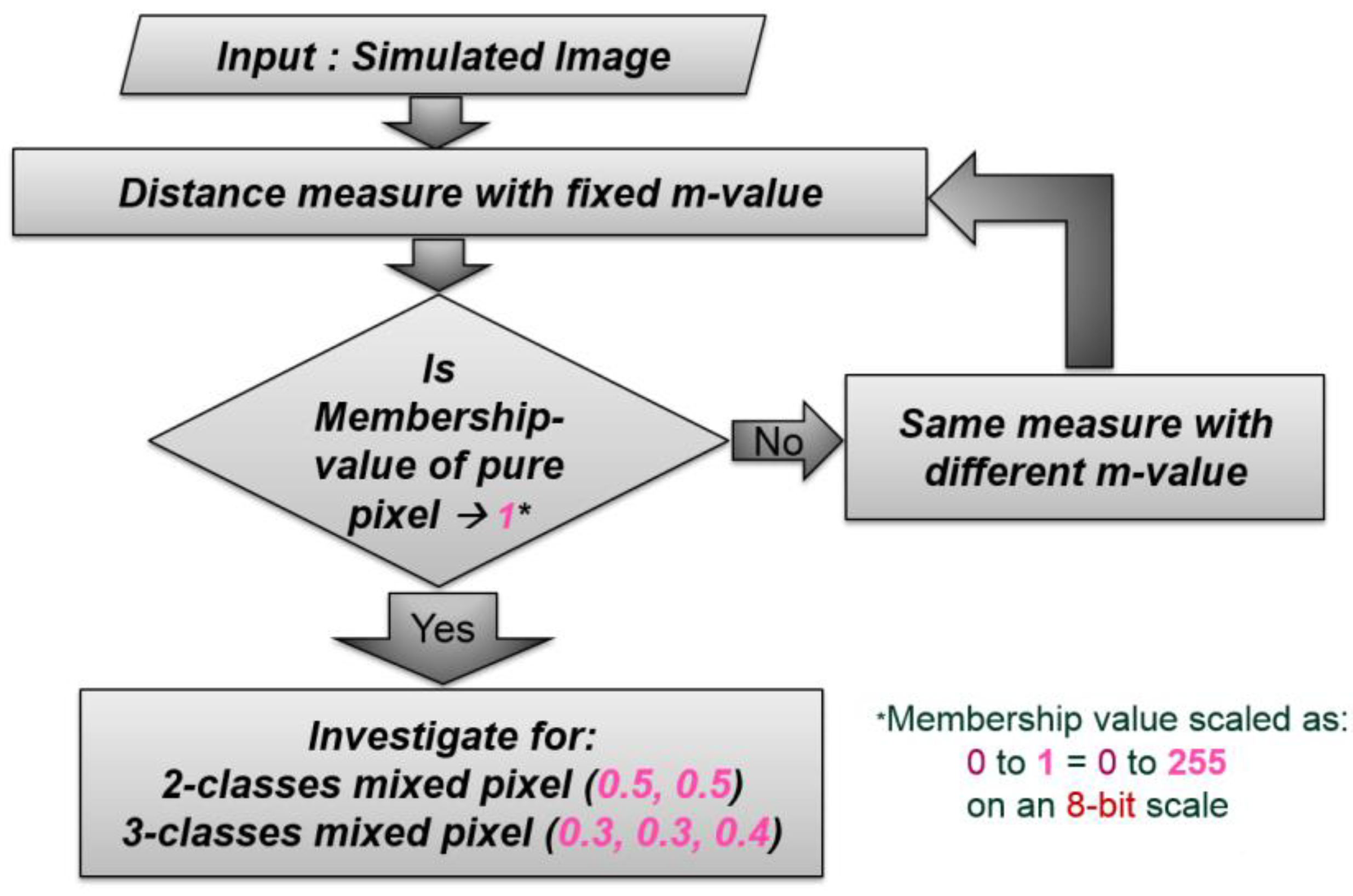
The optimization of the parameters regards the optimization of the weighted-constant ($m^{*}$) for each of the similarity and dissimilarity measures. This optimization was done using simulated image by considering each measure with a fixed $m^{*}$-value and then checking the membership values for (a), (b) and (c) points.

(a)

Pure pixel area (within the class variation as well as membership values must be tending to one and the pixel DN-value should nearly 255 on an 8-bit scale);

if (a) is satisfied, then the behaviour of the similarity measure was checked on;

(b)

Areas where there is a mixing of two classes, membership values must be tending to 0.5 for each class within a pixel (the DN-values should be nearly 127.5 for each class on a 8-bit scale);

(c)

Areas where there is a mixing of three classes, membership values must be tending to 0.3, 0.3 and 0.4 for each class within a pixel (the DN-value should be 76.5, 76.5 and 102 respectively on a 8-bit scale).

The flowchart for the optimization of the weighted constant ($m^{*}$) has been shown in Figure 2. This optimization of the weighted-constant ($m^{*}$) was done for both single as well as composite measures.

2.2. Similarity and Dissimilarity Measures

Considering two sets of measurements X = {x₁, x₂, …, x_n} and Y = {y₁, y₂, …, y_n}, the similarity and dissimilarity between the two sets is a measure of quantifiable dependence or independence between the sets respectively. Measurements of any two objects or phenomena can be represented by X and Y. A similarity measure S is to be considered as a metric if it shows increasing sequences of the value of dependency corresponding to the values in the sequence. The following properties are satisfied by a metric similarity S for all orders of X and Y [19,25]:

• The range is limited: S(X, Y) ≤ S₀, where S₀ is some arbitrarily large number;
• Symmetric: S(X, Y) = S(Y, X);
• Reflexivity: S(X, Y) = S₀, only when X = Y;
• Triangle inequality: S(X, Y) S(Y, Z) ≤ [Z(X, Y) + S(Y, Z)] S(X, Z).

Between the sequences X and Y, the largest possible similarity is S₀.

A dissimilarity measure D is to be considered as a metric if it shows increasing sequences of the value of independency corresponding to the values in the sequence. The following properties are satisfied by a metric dissimilarity D for all orders of X and Y [19,25,26]:

• Non-negativity: D(X, Y) ≥ 0;
• Symmetric: D(X, Y) = D(Y, X);
• Reflexivity: D(X, Y) = 0, only when X = Y;
• Triangle inequality: D(X, Y) + D(Y, Z) ≥ D(X, Z).

Besides having the desirable properties of a metric, a similarity measure can be effective though it may be non-metric. Similarity measures have values ranging from zero to unity, whereas dissimilarity measures have values ranging from zero to infinity (∞), but this value can be normalized to a value ranging from zero to unity. The relationship between similarity (S) and normalized dissimilarity (D) can be shown by the Equation (11):

S = 1 − D

(11)

In few situations, a dissimilarity measure is converted into similarity measure so that it makes the computation easier for further procedures. There are a lot of applications and usages of similarity or dissimilarity measures such as: they help in distinguishing one object from another; the objects can be grouped on the basis of similarity and dissimilarity; a new object can be classified into a group based on the behaviour as per the similarity or dissimilarity measures; thus, further actions and decisions can be planned based on the prediction and structural information of the data. In this study, a total of 12 similarity and dissimilarity measures have been studied with the FCM classifier in single or composite mode. The following section describes the mathematical functions of similarity and dissimilarity measures.

2.2.1. Manhattan

The Manhattan metric estimates the distance based on the sum of the differences between the values of the concerned variables at any location. If we define vector pixel value like X_j = (X_j1, X_j2, X_j3, …, X_jb) and the mean values as V_i = (V_i1, V_i2, V_i3, …, V_ib), then the Manhattan distance can be described as in Equation (12) [27]:

D (X_j, V_i) = Abs (X_j1 − V_i1) + Abs (X_j2 − V_i2) + … + Abs (X_jb − V_ib)

(12)

where, b shows the total amount of bands in the image.

2.2.2. Bray–Curtis

The Bray–Curtis dissimilarity measure is named after J. Roger Bray and John T. Curtis [28]. It is a non-metric dissimilarity approach which is used for many applications and the results are robust and reliable. Bray–Curtis dissimilarity is a modified way of the Manhattan dissimilarity measure. Equation (13) shows the general equation of Bray–Curtis dissimilarity [29]:

$${ \mathrm{d}}^{\mathrm{BCD}}(\mathrm{i}, \mathrm{j}) = \frac{{\sum }_{\mathrm{k} = 0}^{\mathrm{n}-1}\left|{\mathrm{y}}_{\mathrm{i},\mathrm{k}}-{ \mathrm{y}}_{\mathrm{j},\mathrm{k}}\right|}{{\sum }_{\mathrm{k} = 0}^{\mathrm{n}-1}\left|{\mathrm{y}}_{\mathrm{i},\mathrm{k}}+{ \mathrm{y}}_{\mathrm{j},\mathrm{k}}\right|}$$

(13)

In Equation (13), d^BCD is the Bray–Curtis dissimilarity measure between two objects i and j, k is the variable index and n depicts the total amount of variables in y. The outcomes of Bray–Curtis dissimilarity range from zero to unity, where zero defines that the two objects have the similar composition and represent exactly same coordinates and unity defines that the two objects do not have any similarity. The Bray–Curtis dissimilarity is not a distance as it does not satisfy the triangle inequality.

2.2.3. Chessboard

Chessboard is defined as a metric of greatest differences for two vectors along any dimensional coordinates in a vector space1. It is also called Chebyshev (Tchebychev) distance after the name of Pafnuty Chebyshev. In the game of chess, the least moves required by a king to move from a square on a chessboard to another is the same as the Chebyshev distance between the square centres, with a side length of one unit dimension in a 2-dimensional space [30]. It is depicted by the Equation (14) [31]:

D (X_j, V_i) = Max [Abs (X_j1 − V_i1), Abs (X_j2 − V_i2), …, Abs (X_jb − V_ib)]

(14)

where, b shows the total amount of bands in the image.

2.2.4. Canberra

Canberra distance was introduced by [32]. It is a numerical measurement of the distance between two points in a vector space. It has been used for various purposes like a metric for comparison of ranked lists [33] and also in computer security by using intrusion detection [34]. It is similar to the Manhattan distance metric and it is mathematically defined as the absolute difference among the variables of the objects concerned with respect to the summation of the absolute value of the variables before it is summed. Equation (15) shows the working of Canberra distance [34]:

$$\mathrm{D} ({\mathrm{X}}_{\mathrm{j}}, {\mathrm{V}}_{\mathrm{i}}) = \frac{\mathrm{Abs} ({\mathrm{X}}_{\mathrm{j}1}-{\mathrm{V}}_{\mathrm{i}1})}{\mathrm{Abs} \left[{\mathrm{X}}_{\mathrm{j}1}\right]+\mathrm{Abs} \left[{\mathrm{V}}_{\mathrm{i}1}\right]} + \frac{\mathrm{Abs} ({\mathrm{X}}_{\mathrm{j}2}-{\mathrm{V}}_{\mathrm{i}2})}{\mathrm{Abs} \left[{\mathrm{X}}_{\mathrm{j}2}\right]+\mathrm{Abs} \left[{\mathrm{V}}_{\mathrm{i}2}\right]} + \dots + \frac{\mathrm{Abs} ({\mathrm{X}}_{\mathrm{jb}}-{\mathrm{V}}_{\mathrm{ib}})}{\mathrm{Abs} \left[{\mathrm{X}}_{\mathrm{jb}}\right]+\mathrm{Abs} \left[{\mathrm{V}}_{\mathrm{ib}}\right]}$$

(15)

where, b shows the total amount of bands in the image.

2.2.5. Mean Absolute Difference

The mean absolute difference is a statistical measurement of dispersion which is equal to the average value of the absolute difference between two independent numbers acquired from a probability distribution. Mathematically, it can be defined as the summation of the absolute differences between the variables of two independent objects with an identical distribution of the same order and type divided by thetotal number of variables. The mean absolute difference is generally depicted by Δ or as MD. Equation 16 shows the mathematical working of mean absolute difference [35]:

$$\mathrm{D} ({\mathrm{X}}_{\mathrm{j}}, {\mathrm{V}}_{\mathrm{i}}) = \frac{1}{b} [\mathrm{Abs} (\mathrm{X}{\mathrm{j}}_1 - \mathrm{V}{\mathrm{i}}_1) + \mathrm{Abs} (\mathrm{X}{\mathrm{j}}_2 - \mathrm{V}{\mathrm{i}}_2) + \dots + \mathrm{Abs} ({\mathrm{X}}_{\mathrm{jb}} - {\mathrm{V}}_{\mathrm{ib}})]$$

(16)

where, b shows the total amount of bands in the image.

2.2.6. Median Absolute Difference

The Manhattan dissimilarity measure produces an exaggerated value for the distance measure when salt and pepper or impulse noise is present in the image of fixed size with n number of pixels. The Manhattan dissimilarity measure calculates the summation of the absolute difference of the intensity of the corresponding pixels of two different images. The median absolute differences (MAD) may be used instead of the average of absolute differences so that the effect of the noises is reduced on the dissimilarity measure. Although, salt and pepper noise has a considerable effect on the Manhattan measure, it has minimal effect on MAD [36]. MAD is mathematically defined as finding out the differences between the absolute intensities of the corresponding pixels of two images and then taking the median of the orderly data as the dissimilarity measure. Equation (17) [37] shows the mathematical working of MAD:

D (X_j, V_i) = Median [Abs (X_j1 − V_i1) + Abs (X_j2 − V_i2) + … + Abs (X_jb − V_ib)]

(17)

where, b shows the total amount of bands in the image.

2.2.7. Normalized Squared Euclidean

Normalized squared Euclidean calculates the normalized squared Euclidean distance amid two vectors. It normalizes the measure with respect to the contrast of the image. Normalized squared Euclidean requires normalization of the intensities of the pixels before calculating the summation of squared differences among the pixels of two images. Equation (18) [38] shows the mathematical formula:

$$\begin{gathered} \mathrm{D}({\mathrm{X}}_{\mathrm{j}},{ \mathrm{V}}_{\mathrm{i}}) = \frac{\mathrm{Abs}\{{\mathrm{X}}_{\mathrm{j}1}+\frac{1}{\mathrm{b}}(-{\mathrm{X}}_{\mathrm{j}1}-{\mathrm{X}}_{\mathrm{j}2}..-{\mathrm{X}}_{\mathrm{j}\mathrm{b}})-{\mathrm{V}}_{\mathrm{i}1}+\frac{1}{\mathrm{b}}({\mathrm{V}}_{\mathrm{i}1}+{\mathrm{V}}_{\mathrm{i}2}..+{\mathrm{V}}_{\mathrm{i}\mathrm{b}}){\}}^2+\cdots \\ +\mathrm{Abs}\{{\mathrm{X}}_{\mathrm{j}\mathrm{b}}+\frac{1}{\mathrm{b}}(-{\mathrm{X}}_{\mathrm{j}1}-{\mathrm{X}}_{\mathrm{j}2}..-{\mathrm{X}}_{\mathrm{j}\mathrm{b}})-{\mathrm{V}}_{\mathrm{i}\mathrm{b}}+\frac{1}{\mathrm{b}}({\mathrm{V}}_{\mathrm{i}1}+{\mathrm{V}}_{\mathrm{i}2}..+{\mathrm{V}}_{\mathrm{i}\mathrm{b}}){\}}^2}{2\left[\mathrm{Abs}\right\{{\mathrm{X}}_{\mathrm{j}\mathrm{b}}+\frac{1}{\mathrm{b}}(-{\mathrm{X}}_{\mathrm{j}1}-{\mathrm{X}}_{\mathrm{j}2}..-{\mathrm{X}}_{\mathrm{j}\mathrm{b}}){\}}^2+\cdots \\ +\mathrm{Abs}\{{\mathrm{X}}_{\mathrm{j}\mathrm{b}}+\frac{1}{\mathrm{b}}(-{\mathrm{X}}_{\mathrm{j}1}-{\mathrm{X}}_{\mathrm{j}2}..-{\mathrm{X}}_{\mathrm{j}\mathrm{b}}){\}}^2+ \\ \mathrm{Abs}\{{\mathrm{V}}_{\mathrm{i}1}+\frac{1}{\mathrm{b}}(-{\mathrm{V}}_{\mathrm{i}1}-{\mathrm{V}}_{\mathrm{i}2}..-{\mathrm{V}}_{\mathrm{i}\mathrm{b}}){\}}^2+\cdots + \\ \mathrm{Abs}\{{\mathrm{V}}_{\mathrm{i}1}+\frac{1}{\mathrm{b}}(-{\mathrm{V}}_{\mathrm{i}1}-{\mathrm{V}}_{\mathrm{i}2}..-{\mathrm{V}}_{\mathrm{i}\mathrm{b}}){\}}^2]} \end{gathered}$$

(18)

where, b shows the total amount of bands in the image.

2.2.8. Cosine

Cosine similarity measure calculates the cosine of the angle between two vectors present in an inner product space. The value of the cosine of the angle ranges from −1 to 1. The Cosine measure at zero degrees angle is 1 and it decreases at any angle other than zero. Thus, vectors of similar orientation have a cosine similarity of 1, vectors at a right angle have a cosine similarity of 0 and vectors which are exactly opposite to each other have a cosine similarity of −1. However, generally cosine similarity is used in positive space, so the values are bounded from 0 to 1. Cosine similarity is used for high-dimensional positive spaces. Cosine similarity gives a measurement of similarity between two vectors with respect to each other [39]. This technique is used for the calculation of cohesion among the clusters in the field of data mining [40]. Equation (19) [41] shows the mathematical formula of cosine similarity:

$$\mathrm{D}({\mathrm{X}}_{\mathrm{j}},{\mathrm{V}}_{\mathrm{i}}) = 1- \frac{{\mathrm{X}}_{\mathrm{j}1}{\mathrm{V}}_{\mathrm{i}1}+{ \mathrm{X}}_{\mathrm{j}2}{\mathrm{V}}_{\mathrm{i}2}+\dots +{ \mathrm{X}}_{\mathrm{jb}}{\mathrm{V}}_{\mathrm{ib}}}{\sqrt{\mathrm{Abs} \left[{\mathrm{X}}_{\mathrm{j}1}{]}^2+\dots +\mathrm{Abs} \right[{\mathrm{X}}_{\mathrm{jb}}{]}^2 } \sqrt{\mathrm{Abs} \left[{\mathrm{V}}_{\mathrm{i}1}{]}^2+\dots +\mathrm{Abs} \right[{\mathrm{V}}_{\mathrm{ib}}{]}^2 }}$$

(19)

where, b shows the total amount of bands in the image.

2.2.9. Correlation

Correlation similarity is a measure of finding the correlation between the two vectors. It uses a standardized angular separation method by centring the coordinates towards its mean vector value. The correlation output is within the range of −1 to 1. The correlation output is normalized for a positive vector space, hence the output ranges from 0 to 1. It is a similarity measure rather than a distance measure. The similarity between two vectors is computed by using the Pearson-r correlation [42]. Equation (20) [43] shows the correlation mathematical formula:

$$\begin{gathered} \mathrm{D}({\mathrm{X}}_{\mathrm{j}},{ \mathrm{V}}_{\mathrm{i}}) = \frac{\left[\right\{{\mathrm{X}}_{\mathrm{j}\mathrm{b}}+\frac{1}{\mathrm{b}}(-{\mathrm{X}}_{\mathrm{j}1}-{\mathrm{X}}_{\mathrm{j}2}...-{\mathrm{X}}_{\mathrm{j}\mathrm{b}})\left\}\right\{{\mathrm{V}}_{\mathrm{i}1}+\frac{1}{\mathrm{b}}(-{\mathrm{V}}_{\mathrm{i}1}-{\mathrm{V}}_{\mathrm{i}2}...-{\mathrm{V}}_{\mathrm{i}\mathrm{b}})\}+\cdots \\ +\{{\mathrm{X}}_{\mathrm{j}\mathrm{b}}+\frac{1}{\mathrm{b}}(-{\mathrm{X}}_{\mathrm{j}1}-{\mathrm{X}}_{\mathrm{j}2}...-{\mathrm{X}}_{\mathrm{j}\mathrm{b}})\left\}\right\{{\mathrm{V}}_{\mathrm{i}\mathrm{b}}+\frac{1}{\mathrm{b}}(-{\mathrm{V}}_{\mathrm{i}1}-{\mathrm{V}}_{\mathrm{i}2}...-{\mathrm{V}}_{\mathrm{i}\mathrm{b}})\left\}\right]}{\sqrt{\mathrm{Abs}[{\mathrm{X}}_{\mathrm{j}1}+\frac{1}{\mathrm{b}}(-{\mathrm{X}}_{\mathrm{j}1}\cdots -{\mathrm{X}}_{\mathrm{j}\mathrm{b}}){]}^2+..+\mathrm{Abs}[{\mathrm{X}}_{\mathrm{j}\mathrm{b}}+\frac{1}{\mathrm{b}}(-{\mathrm{X}}_{\mathrm{j}1}\cdots -{\mathrm{X}}_{\mathrm{j}\mathrm{b}}){]}^2} \\ \sqrt{\mathrm{Abs}[{\mathrm{V}}_{\mathrm{i}1}+\frac{1}{\mathrm{b}}(-{\mathrm{V}}_{\mathrm{i}1}\cdots -{\mathrm{V}}_{\mathrm{i}\mathrm{b}}){]}^2+\cdots +\mathrm{Abs}[{\mathrm{V}}_{\mathrm{j}\mathrm{b}}+\frac{1}{\mathrm{b}}(-{\mathrm{V}}_{\mathrm{i}1}\cdots -{\mathrm{V}}_{\mathrm{i}\mathrm{b}}){]}^2}} \end{gathered}$$

(20)

where, b shows the total amount of bands in the image.

2.2.10. Euclidean

Euclidean distance is the normal distance between two objects in a metric space. The measure associated is known as the Euclidean measure. Reference [13] introduced this measure with FCM classifier in the form of an identity matrix. Equation (21) shows the mathematical form of the Euclidean measure used for FCM:

D (X_j, V_i) = I, where I is the identity matrix

(21)

2.2.11. Mahalanobis

Mahalanobis distance was introduced by [44]. It measures the distance amid a point and a distribution. The distance tends to zero as the point tends to move towards the mean of the distribution and vice versa. Reference [13] used this distance in the form of a variance–covariance matrix C_j for FCM. Equation (23) shows the mathematical formulation used for FCM:

$$\mathrm{D} ({\mathrm{X}}_{\mathrm{j}}, {\mathrm{V}}_{\mathrm{i}}) = {\sum }_{\mathrm{i} = 0}^{\mathrm{N}}({\mathrm{x}}_{\mathrm{i}}-{ \mathrm{v}}_{\mathrm{j}}){\mathrm{C}}_{\mathrm{j}}^{-1} {({\mathrm{x}}_{\mathrm{i}}-{ \mathrm{v}}_{\mathrm{j}})}^{\mathrm{T}}$$

(22)

where,

$${\mathrm{v}}_{\mathrm{j}} = {\displaystyle \sum }_{\mathrm{i} = 1}^{\mathrm{N}}{\mathrm{x}}_{\mathrm{i}}/\mathrm{N}$$

(23)

2.2.12. Diagonal Mahalanobis

Diagonal Mahalanobis measure is the diagonal matrix D_j consisting of diagonal elements which are the eigenvalues of the variance–covariance matrix C_j shown in Equations (22)–(24) [13] shows the mathematical form of the diagonal measure:

$$\mathrm{D} ({\mathrm{X}}_{\mathrm{j}}, {\mathrm{V}}_{\mathrm{i}}) = {\mathrm{D}}_{\mathrm{j}}^{-1}$$

(24)

2.2.13. Composite Measure

The composite measure can be generated by using any of the two measures (similarity or dissimilarity) in combination by choosing a weighting component λ. By using a combination of two among the 12 similarity or dissimilarity measures, a composite measure can be created as in Equation (25).

$${\mathrm{D}}_{\mathrm{c}} ={ \mathsf{\lambda }\mathrm{D}}_{\mathrm{a}}+(1- \mathsf{\lambda }){\mathrm{D}}_{\mathrm{b}}$$

(25)

where, D_c is Composite measure and λ is a weighting component, 0 ≤ λ ≤ 1, D_a and D_b can be any similarity or dissimilarity measure.

2.3. Accuracy Assessment

Assessment is a very important step to quantify the results of the outputs and to compare them with other techniques of classification [45]. The error matrix, confusion matrix or contingency table is one of the ways to showcase the accuracy of results obtained through classification. The error matrix produces the settlement of accuracy assessment between the data that are classified and the data that are used as a reference along with wrongly classified outputs. Several statistical processes such as the Kappa coefficient, user’s accuracy, producer’s accuracy and overall accuracy have been introduced on the basis of the error matrix. These processes are used to sum up all the statistics about accuracy assessment. In the sole case of hard classification, the error matrix is used for the accuracy assessment as in hard classification a single pixel belongs to a single class and, not when a pixel may belong to two or more classes [46]. In the case of soft classification, other methods like fuzzy error matrix (FERM), sub-pixel confusion uncertainty matrix (SCM), etc. were introduced for assessing the accuracy [11,47,48]. Fuzzy error matrix was introduced for measuring the accuracy of soft classifiers. The following section describes the methods used for accuracy assessment of soft classified outputs.

2.4. Fuzzy Error Matrix (FERM)

In FERM, both the referenced data and the classified data are in the form of a fuzzy set, having membership values ranging between 0 and 1. FERM is created on the basis of the MIN operator which offers a maximum overlap among the classified and the referenced data at a sub-pixel level. Equation (26) [11] shows the mathematical formulation for the FERM operator:

$${\mathsf{\mu }}_{{\mathrm{C}}_{\mathrm{m}}\cap {\mathrm{R}}_{\mathrm{n}}}(x) = \min ({\mu }_{{\mathrm{C}}_{\mathrm{m}}}(x), { \mathsf{\mu }}_{{\mathrm{R}}_{\mathrm{n}}}(x))$$

(26)

where, R_n depicts the membership value from the referenced data, in the form of a set, which is allotted to class n, C_m depicts the membership value from the classified data, also in the form of a set, which are allotted to class m and the membership value of a pixel with respect to the classes is shown by μ. The overall accuracy is the primitive form of statistics gathered from an accuracy assessment. In the case of FERM, the overall accuracy is measured by calculating the sum of the diagonal components divided by the total membership value of the referenced data. Equation (27) [49] shows the mathematical formulation:

$${ \mathrm{OA}}_{\mathrm{FERM}} = \frac{{\sum }_{\mathrm{i} = 1}^{\mathrm{c}}\mathrm{M}(\mathrm{I}, \mathrm{j})}{{\sum }_{\mathrm{i} = 1}^{\mathrm{c}}{\mathrm{R}}_{\mathrm{j}}}$$

(27)

Here, OA depicts the overall accuracy, M(i, j) depicts the elements of the mth class of the soft classified result and nth class of the soft reference record, c depicts the total number of classes and R_j depicts the total summation of the membership value of n class in the soft reference data.

2.5. Subpixel Confusion Uncertainty Matrix (SCM)

Determination of the true overlap between classes which are on the basis of fractional land cover is challenging. This kind of situation is known as sub-pixel area allocation problem [46]. The spatial distribution of the classes determines the minimum or maximum overlap of the classes in a pixel. This kind of problem gives rise to solutions such as a unique solution or no solution. For, a unique solution, there is a chance of overestimation or underestimation of classes and hence, the sub-pixel confusion matrix can be uniquely defined. For the case of no solution, as there is a lack of unique solution, hence the solutions are depicted by confusion intervals. SCM has confusion intervals, which are shown as central value ± maximum error. The confusion matrix produced for a soft classifier output satisfies the following [46]:

• Property of diagonalization: if the data that are considered is equal to the classified data, then the matrix is a diagonal matrix.
• Property of marginal sums: the total summation of the marginal equals the total values both from the data that are assessed and the classified data.

3. Study Area and Materials Used

3.1. Study Area

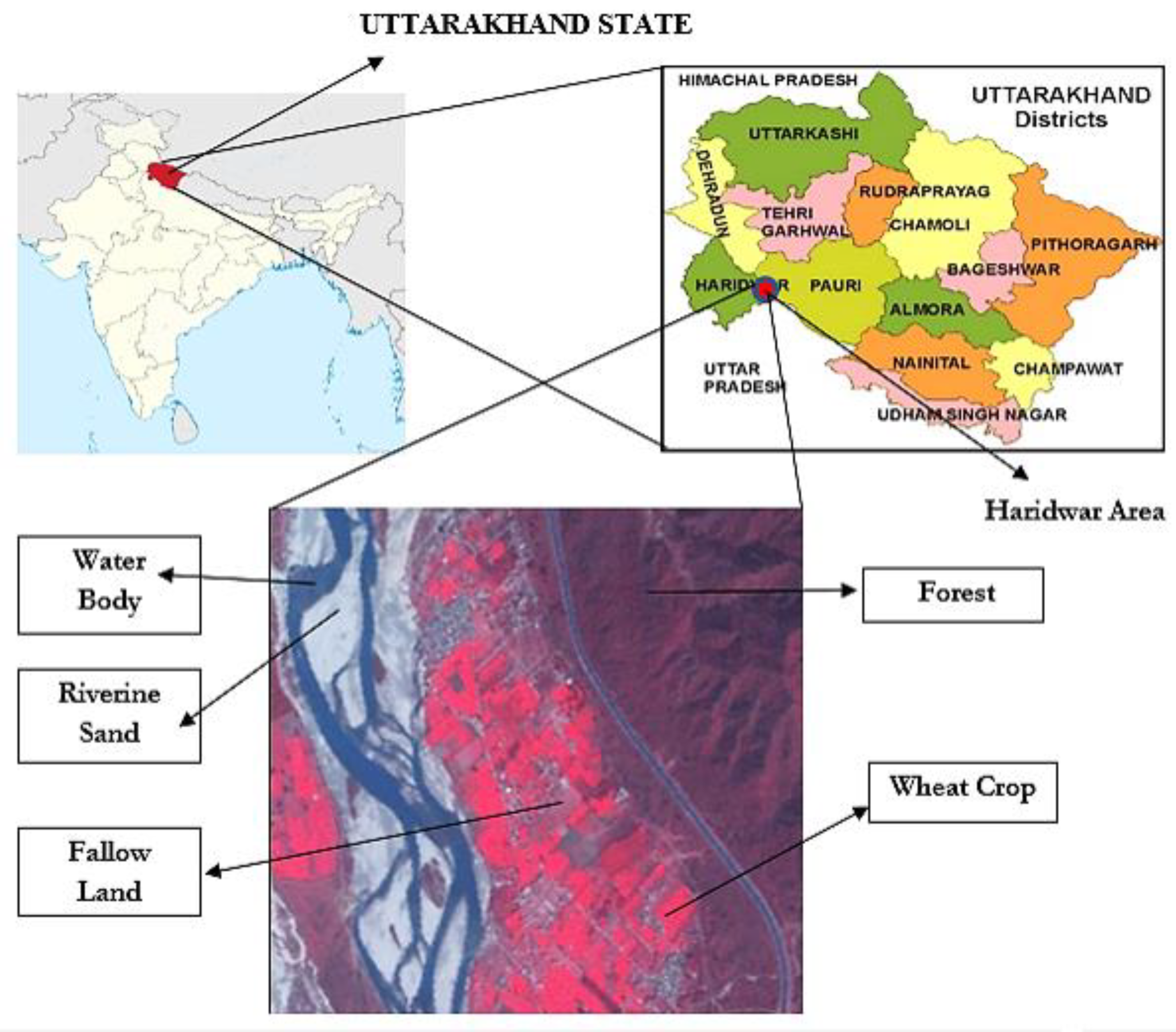
The study area selected for this project work was in the district of Haridwar, Uttarakhand, and is shown in Figure 3. The district shares its boundaries with Dehradun in the north, Pauri Garhwal in the east while, west and south are bounded by districts of Uttar Pradesh. The central latitude and longitude of the district are 29.956°N and 78.170°E respectively. The coverage of the area is 2.664 km × 2.192 km in the east to west and north to south direction respectively. The land is fertile with river Ganga flowing through the district and agriculture remains the mainstay of the district. Five classes that were considered as follows: water, riverine sand, wheat crop, forest, and fallow land. This study area was selected due to the diversity of land-use classes, such as vegetation type (wheat), riverine sand, forest, fallow land and water. There is also the presence of mixed pixels at the boundaries of the classes and this will help to examine the capacity of FCM classifier with different similarity and dissimilarity measures for classification. Ground truth data of the study area were available as the field visit was conducted on 16 March 2015. Data sets from the sensors Formosat-2 and Landsat-8 were also available in the same time frame as to check the image to image accuracy of the classifier. Formosat-2 and Landsat-8 sensor images were acquired on 21 February 2015 and 12 February 2015, respectively.

3.2. Material Used

In this research work, multispectral images of 8 m and 30 m resolution of Formosat-2 and Landsat-8 satellites were used. The soft fractional outputs of finer resolution Formosat-2 images were used to validate the soft fractional outputs of Landsat-8.

Table 1. Formosat and Landsat satellite specification.

Specification	FORMOSAT-2	LANDSAT-8
Spatial Resolution (m)	8 m	30 m
Spectral Resolution	B1: 0.45–0.52 µm (Blue) B2: 0.52–0.60 µm (Green) B3: 0.63–0.69 µm (Red) B4: 0.76–0.90 µm (Near-infrared)	B1: 0.450–0.515 µm (Blue) B2: 0.525–0.600 µm (Green) B3: 0.630–0.680 µm (Red) B4: 0.845–0.885 µm (Near-infrared)
Sensor Footprint	24 km × 24 km	185 km × 170 km
Return Interval	Daily	After every 16 days
Orbiting Height	888 km	438 miles = 705 km (approx.)
Orbiting Type	Sun-synchronous	near-polar, sun-synchronous orbit

shows the specifications of the satellite data used:

3.3. The Simulated Image

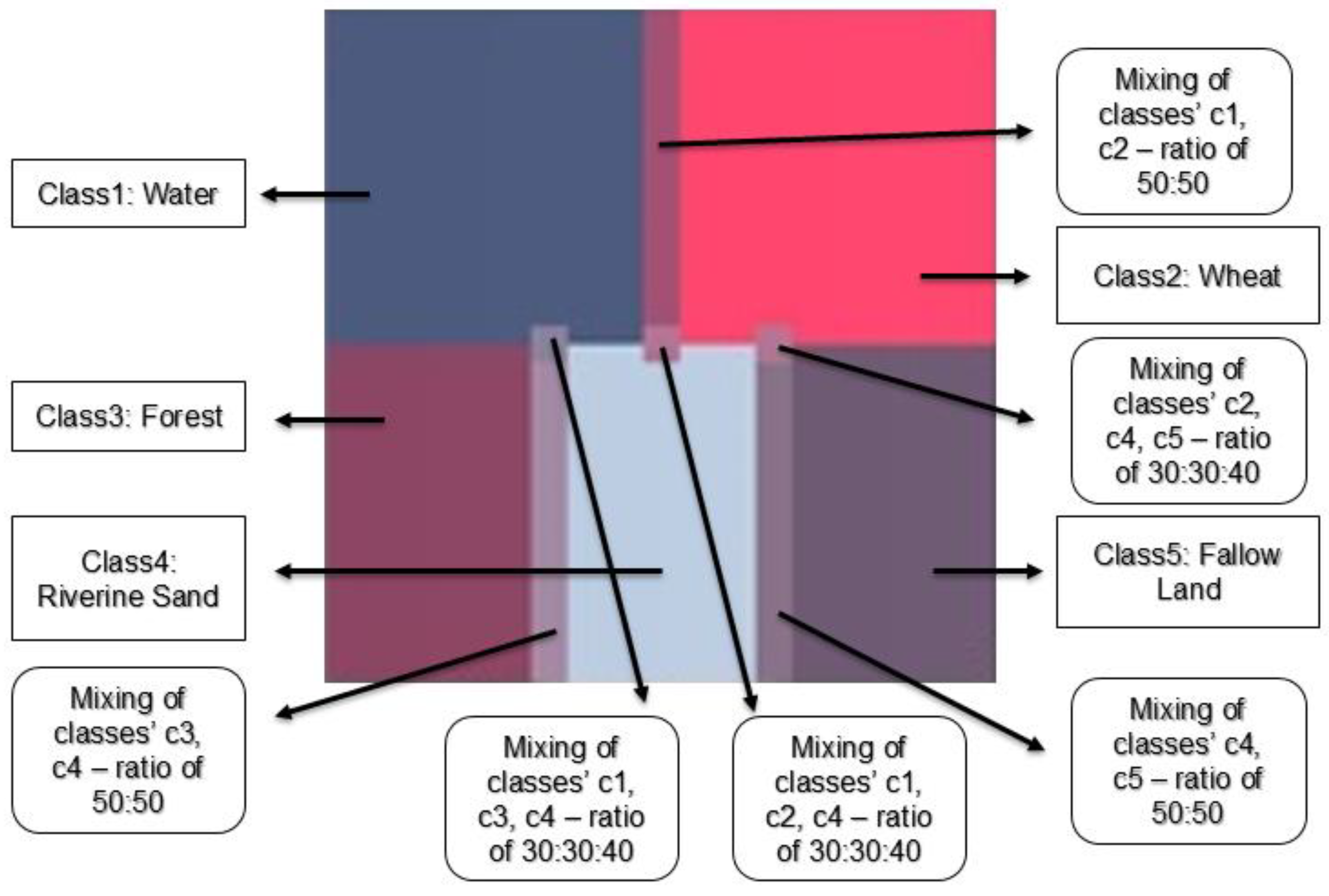
In this research work, simulated image of multi-spectral data (4 bands) of Formosat-2 has been taken as reference data and a simulated image of Landsat-8 has also been taken as a set to study the performance of all the measures i.e., Euclidean, Mahalanobis, diagonal Mahalanobis, Cosine, correlation, Canberra, Manhattan, chessboard, Bray–Curtis, mean absolute difference, median absolute difference and normalized squared Euclidean with FCM classifier. Simulated Formosat-2 and Landsat-8 images contain five classes: water body, wheat, forest, fallow land and riverine sand.

In the simulated image, we have intentionally mixed classes in a specific ratio and also created a small variation within the class. Based on these controlled conditions the ability to handle the mixed pixel problem and detecting the intra-class pixel value variation were tested on the simulated image. Details of the simulated images were explained in Figure 4.

4. Results

4.1. Identification of Best Measure and Estimation of the Parameters

The behavioural characteristics of the developed FCM were studied in details using the simulated image. This simulated image was developed to estimate the parameters and also to check the accuracy of the FCM classification. The simulated image was developed according to the study area selected, containing all the classes present in the study area and within the class variation was incorporated to check the capability of the FCM classifier to detect variation at an intra-class level. The simulated image has been generated for the Formosat-2 image as well as for the Landsat-8 image. The membership grade of a pixel with respect to a class in a fractional image ranges from 0 to 1. In order to eliminate the cumbersome process of handling decimal digits between 0 and 1, the membership grades were up-scaled to 8-bit values ranging from 0 to 255. In FCM, the membership grade of zero for a pixel denotes that the pixel does not belong to a concerned class and the membership grade of 255 for a pixel denotes that the pixel completely belongs to the concerned class. In this research work, the fractional images from Formosat-2 dataset have been used as the referenced images to calculate the accuracy of the Landsat-8 dataset.

The best parameter value of weighted constant ($m^{*}$) was estimated for the developed FCM algorithm with the simulated image, as the input of the image and the expected output was also known. This optimized parameter of weighted constant ($m^{*}$) was also used to check the effect of change of the degree of fuzziness on the accuracy. The weighted-constant or fuzzifier was optimized within the value ranging from 1.10 to 3.00. By, using the optimization of parameter technique, the best two measures out of all 12 measures were chosen to form a composite measure. The optimization of the parameter value of weighed constant ($m^{*}$) was also estimated for supervised FCM algorithm with this composite measure. Lastly, with this optimized parameter value of weighted constant (m*) the best similarity or dissimilarity measure (single or composite) function was implemented with the supervised FCM classification and the accuracy assessment of the obtained classified results were obtained.

The simulated image was used to identify for optimization of the weighted constant ($m^{*}$) parameter and also to find out the best similarity or dissimilarity measures for both Formosat-2 and Landsat-8 datasets. This optimized parameter of ($m^{*}$) along with the best similarity or dissimilarity measure function was used for image to image accuracy assessment of the image with coarser resolution, Landsat-8. The aforementioned technique was also used to optimize the weighted-constant ($m^{*}$) parameter and also to find the best similarity or dissimilarity measure for the Landsat-8 image. Accuracy assessment techniques like FERM and SCM were used to measure the accuracy of the classified images.

4.1.1. Fuzzifier or Weighted Constant ($m^{*}$)

Here, the study was executed with Formosat-2 simulated image with five different classes. Firstly, the FCM algorithm was implemented with five different classes namely fallow land, forest, riverine sand, water and wheat to optimize the weighted constant ($m^{*}$) for the FCM algorithm on various similarity and dissimilarity measures. A comparative exploration was done on the effect of the fuzzifier ($m^{*}$) on each similarity measures incorporated into the FCM algorithm.

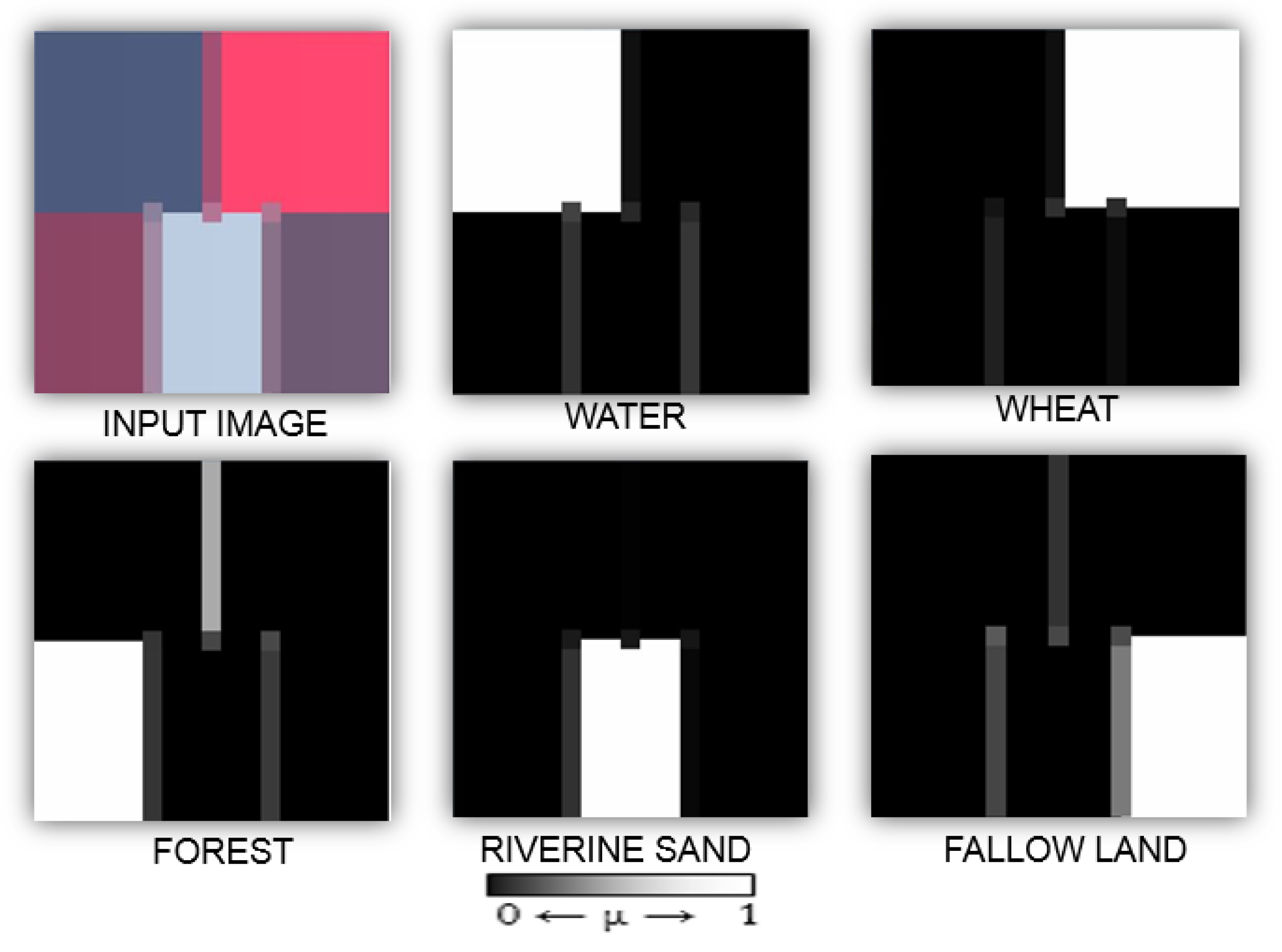
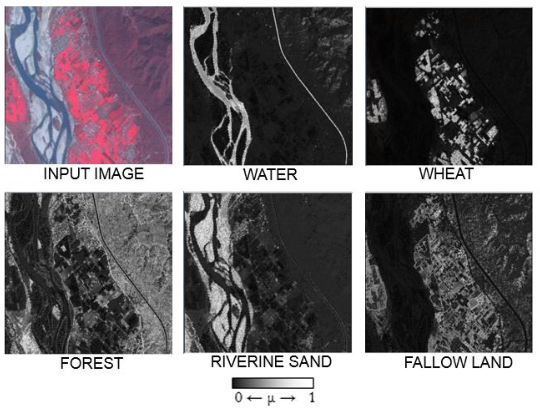
We have implemented the FCM classification algorithm for all the measures on the simulated image of the Formosat-2 dataset. The value for the weighted-constant or fuzzifier ($m^{*}$) was carefully chosen on the basis of the results obtained in the classification. In the results, the criterion for optimality was based on the classification of the pure pixels, whose value should reach the target values of 255 and 254 respectively with minimum intra-class variation for that concerned class. Along with the aforementioned criteria, the mixed pixel should also be classified according to the target values. The results obtained showed that for the Formosat-2 simulated image the optimal value of $m^{*}$ was achieved at $m^{*}$ equals to 2.7 for Cosine measure, which was the best measure. Figure 5 shows the outputs of the FCM algorithm with a simulated image for Cosine measure with $m^{*}$ equal to 2.7. In the simulated image, mixed pixels were simulated with two types of variations, one with the composition of 50:50 (as shown in Figure 4) between two different classes and another with the arrangement of 30:30:40 (as shown in Figure 4) among three different classes. The target membership value expected for a pixel belonging completely to a class must be close to 255 (on an 8-bit scale) and the target membership value for a pixel of the mixed pixels of two different classes must be close to 127.5 (on an 8-bit scale) i.e., 50% of the full membership value of a pixel belonging to a concerned class and the target membership value for a pixel of the mixed pixels of three different classes must be close to 76.5, 76.5 and 102 (on an 8-bit scale) i.e., 30%, 30% and 40% of the full membership value of a pixel belonging to a concerned class, respectively.

Table 2. Shows the results of all the measures while handling the pure pixel classes and also its behaviour within the class variation (Membership value was calculated on 8-bit scale i.e., the target values for a class were 255 and 254 (with a variation of 1 within the class)). The results obtained for Cosine measure are shown in bold.

Measures (with m*-Value)	Water	Wheat	Forest	Riverine-Sand	Fallow-Land	Total Variation of Pure Pixel Class
Canberra (1.9)	247 − 239 = 8	249 − 242 = 7	246 − 238 = 8	253 − 252 = 1	246 − 237 = 9	33
Cosine (2.7)	253 − 252 = 1	254 − 253 = 1	253 − 252 = 1	254 − 254 = 0	253 − 252 = 1	4
Euclidean (2.5)	253 − 250 = 3	254 − 253 = 1	253 − 250 = 3	254 − 253 = 1	252 − 248 = 4	12
Chessboard (1.9)	252 − 249 = 3	253 − 252 = 1	251 − 248 = 3	253 − 251 = 2	251 − 246 = 5	14
Mean Absolute Distance (1.9)	248 − 240 = 8	251 − 246 = 5	248 − 241 = 7	253 − 251 = 2	246 − 237 = 9	31
Diagonal Measure (2.5)	253 − 250 = 3	254 − 253 = 1	253 − 250 = 3	254 − 253 = 1	252 − 248 = 4	12
Median Absolute Distance (1.9)	250 − 246 = 4	252 − 250 = 2	250 − 246 = 4	253 − 251 = 2	249 − 243 = 6	18
Manhattan (1.9)	248 − 240 = 8	251 − 246 = 5	248 − 241 = 7	253 − 251 = 2	246 − 237 = 9	31
Bray-Curtis (1.9)	247 − 240 = 7	241 − 247 = 4	248 − 240 = 8	253 − 252 = 1	246 − 237 = 9	29
Correlation (2.5)	0	0	0	0	0	-
Mahalanobis (2.5)	124 − 122	252 − 249	124 − 122	254 − 253	237 − 201	-
Normalised Squared Euclidean (2.7)	255	255	254	0	254	-

shows the results of all the measures while handling the pure pixel classes and also its behaviour for within the class variation. As mentioned before, the intra class variation for the simulated image of Formosat-2 was 1, hence the target values for all the measures were 255 and 254 (as shown in the table as 255–254), respectively. For detection of pure pixels along with the variation, Cosine measure outperforms all other measures. Cosine measures reach a value of 253–252 for the class water, the best among all the other measures, and similarly for other classes like: 254–253 for the class wheat, 253–252 for the class forest, 254–254 for the class riverine sand and 253–252 for the class fallow land. There are a few measures that did not perform well for this study of pure pixel detection along with the variation. The measures like correlation, Mahalanobis and normalised squared Euclidean did not perform well. The correlation measure could not classify the pure pixels and showed value zero for all the classes. The Mahalanobis measure performed well for classes’ wheat, riverine sand and fallow land, but were not the best results. However, it showed results like 124–122 for both class water and class forest, which were not close to the desired target values of 255–254. The normalised squared Euclidean measure also did not perform well; it detected the pure pixels for classes like water, wheat, forest and fallow land, but could not detect the class riverine sand like correlation measure. Although it detected the pure pixels for some classes, it failed to detect the intra class variation. It detected the classes’ of wheat and water with the value of 255 and did not detect the variation at all. Similarly, for the classes’ forest and fallow land, it detected them with a single value of 254. Hence, the intra-class variation for the measures like correlation, Mahalanobis and normalised squared Euclidean was not calculated and represented with a hyphen (-). Out all the measures, Cosine measure shows the least intra-class variation.

Table 3. Shows the results of all the measures while handling the mixed pixel containing two classes (membership value was calculated on 8-bit scale i.e., the target value for each class was 127.5, respectively).

Measures (with m*-Value)	Riverine Sand-Forest	Riverine Sand-Fallow Land	Water-Wheat
Canberra (1.9)	68-46	29-76	35-54
Cosine (2.7)	69-33	46-154	14-20
Euclidean (2.5)	50-52	18-94	30-29
Chessboard (1.9)	53-54	26-105	28-28
Mean Absolute Distance (1.9)	51-52	20-77	39-40
Diagonal Measure (2.5)	50-52	18-94	30-29
Median Absolute Distance (1.9)	49-50	22-97	37-37
Manhattan (1.9)	51-52	20-77	39-40
Bray-Curtis (1.9)	65-47	28-74	37-44
Correlation (2.5)	19-26	12-210	10-39
Mahalanobis (2.5)	32-34	3-18	57-49
Normalised Squared Euclidean (2.7)	24-24	15-211	16-16

shows the results of all the measures while handling the mixed pixels with two different classes. Here, the target value for each class is 127.5 due to the equal ratio (0.5 for each class) mixture of the classes i.e., 127.5 (50% of the pure pixel target value of 255 and shown in the table as 127.5–127.5 for each measure in accordance with the corresponding classes) for each class respectively. Here, none of the measures could provide any significant result.

Table 4. Shows the results of all the measures while handling the mixed pixel containing three classes (membership value was calculated on 8-bit scale i.e., the target values for each class were 76.5, 76.5 and 102, respectively).

Measures (with m*-Value)	Water-Forest-Riverine Sand	Water-Riverine Sand-Wheat	Riverine Sand-Fallow Land-Wheat
Canberra (1.9)	52-52-49	49-49-48	47-60-47
Cosine (2.7)	32-23-78	27-45-23	48-69-23
Euclidean (2.5)	61-53-35	44-33-49	31-65-47
Chessboard (1.9)	50-55-41	33-40-48	40-55-45
Mean Absolute Distance (1.9)	59-58-36	55-36-47	34-62-45
Diagonal Measure (2.5)	61-53-35	44-33-49	31-65-47
Median Absolute Distance (1.9)	58-50-39	45-34-49	34-63-46
Manhattan (1.9)	59-58-36	55-36-47	34-62-45
Bray-Curtis (1.9)	55-53-48	50-48-48	45-58-47
Correlation (2.5)	60-16-51	6-6-15	3-7-8
Mahalanobis (2.5)	24-24-13	27-17-151	14-28-161
Normalised Squared Euclidean (2.7)	41-20-61	13-15-9	20-42-10

shows the results of all the measures while handling the mixed pixels with three different classes. Here, the target value for the classes are 76.5, 76.5 and 102 (shown in the table as 76.5–76.5–102 for each measure in accordance with the corresponding classes), respectively. This is done by mixing the classes in the ration of 0.3, 0.3 and 0.4 respectively (30% of the pure pixel target value of 255 is 76.5 and 40% of the pure pixel target value of 255 is 102). Here also, none of the measures completely showed any significant results.

The results obtained for the Formosat-2 simulated image as shown in Table 2 depicting that Cosine measure at m* equals 2.7 shows the best result among all the similarity measures for handling the pure pixels in an image and also can detect the intra-class variation properly. The results shown in Table 3 and Table 4 show that the measures were unable to handle the mixed pixels properly. This can be due to the inefficiency of FCM classifier in handling noise. Here, the mixture of two or more classes creates noise for the other concerned class during classification and hence, the developed FCM algorithm cannot handle the mixed pixels properly. A similar analysis was done on the simulated image of Landsat-8, which resulted in Cosine measure with m* equals 2.7 showed the best result while handling the pure pixels in an image and also while detecting the intra-class variation. Figure 6 shows the output results of Cosine measure with m* equals 2.7 for the Formosat-2 real image.

4.1.2. Weighting Component (λ) for Composite Measure

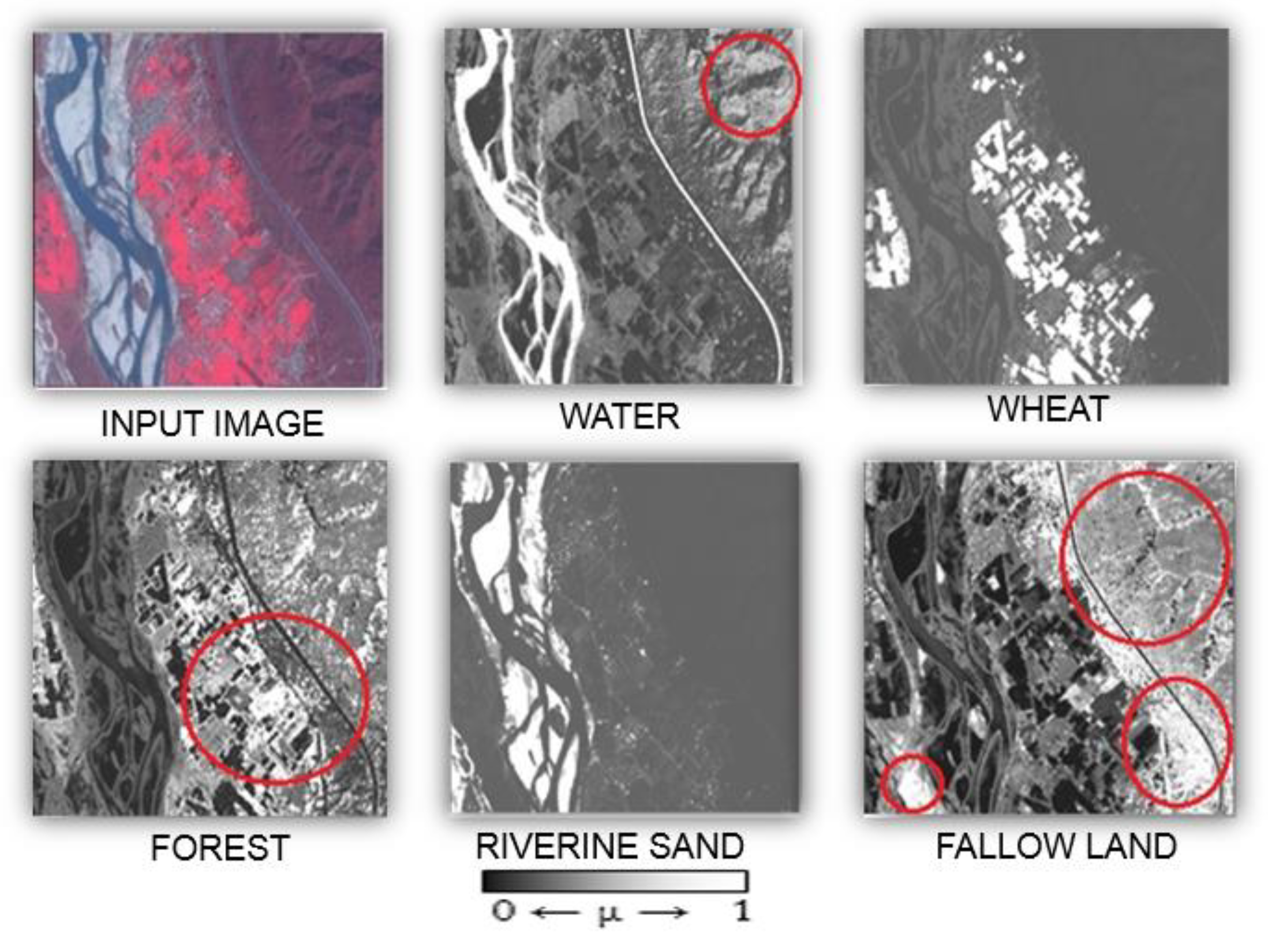
A composite measure requires a weighting component (λ), which provides weight λ to a measure D_a and 1 − λ to another measure D_b. For, a composite measure it was essential to optimize both the parameters of λ and m. The values considered for λ were ranging from 0.10 to 0.90. However, the classification may result in misclassified outputs when the weight set for a measure D_a is greater than D_b. This kind of misclassification arises if the performance of D_a is better than D_b and with a larger value of weighting component (λ) to D_b in a composite situation will result in a measure with inferior results. Figure 6 shows that fallow-land and forest classes have misclassification in the results. The two best measures obtained from the results shown in Table 2, Table 3 and Table 4 were Cosine and Euclidean. These two measures were used to make the composite measure. The results obtained after optimization of both parameters m and λ on the simulated images show that the composite measure of Cosine and Euclidean were optimized at m* equals 2.5. However, there was no significant change observed while changing the value of λ from 0.10 to 0.99.

Table 5. The comparative results of the best single similarity measures and the composite measure while handling the pure pixel classes and also its behaviour within the class variation (membership value was calculated on 8-bit scale i.e., the target values for a class is 255 and 254 (with a variation of 1 within the class)).

Measures (with m-Value)	Water	Wheat	Forest	Riverine-Sand	Fallow-Land	Total Variation of Pure Pixel Class
Cosine (2.7)	253 − 252 = 1	254 − 253 = 1	253 − 252 = 1	254 − 254 = 0	253 − 252 = 1	4
Euclidean + Cosine (2.5)	253 − 250 = 3	254 − 253 = 1	253 − 250 = 3	254 − 253 = 1	252 − 248 = 4	12

,

Table 6. The comparative results of the best single similarity measures and the composite measure while handling the mixed pixel containing two classes (membership value was calculated on 8-bit scale i.e., the target values for each class was 127.5, respectively).

Measures (with m-Value)	Riverine Sand-Forest	Riverine Sand-Fallow Land	Water-Wheat
Cosine (2.7)	69-33	46-154	14-20
Euclidean + Cosine (2.5)	50-52	18-94	30-29

and

Table 7. The comparative results of the best single similarity measures and the composite measure while handling the mixed pixel containing three classes (membership value was calculated on 8-bit scale i.e., the target values for each class were 76.5, 76.5, 102, respectively).

Measures with m-Value	Water-Forest-Riverine Sand	Water-Riverine Sand-Wheat	Riverine Sand-Fallow Land-Wheat
Cosine (2.7)	32-23-78	27-45-23	48-69-23
Euclidean + Cosine (2.5)	61-53-35	40-33-49	31-65-47

show the comparison between the results of the best single measure and the results of the composite measure. In Figure 7, it was also observed that the fallow land was misclassified as forest and also forest was misclassified with water and fallow land.

4.2. Results of FCM Classifier Using α-Cuts with Single Measure

Although fuzzy clustering techniques with cluster cores have good clustering characteristics, there can be difficulties in cluster cores produced by FCM in case non-spherical shape clusters. For example, the cluster cores of two overlapping clusters (line structure) cannot be determined by FCM [23]. So, to describe the general core of the clusters of any shape, α-cut has been incorporated in the FCM algorithm. The cluster cores generated by FCM was such that if the distance between the pixel and the cluster centre of the concerned class was less than a defined threshold (α-cut value), then that pixel would be belonging to that class with membership grade value of 1. In this study, the α-cut value was taken in the range from 0.5 to 0.9 with an interval of 0.1, as suggested by [23].

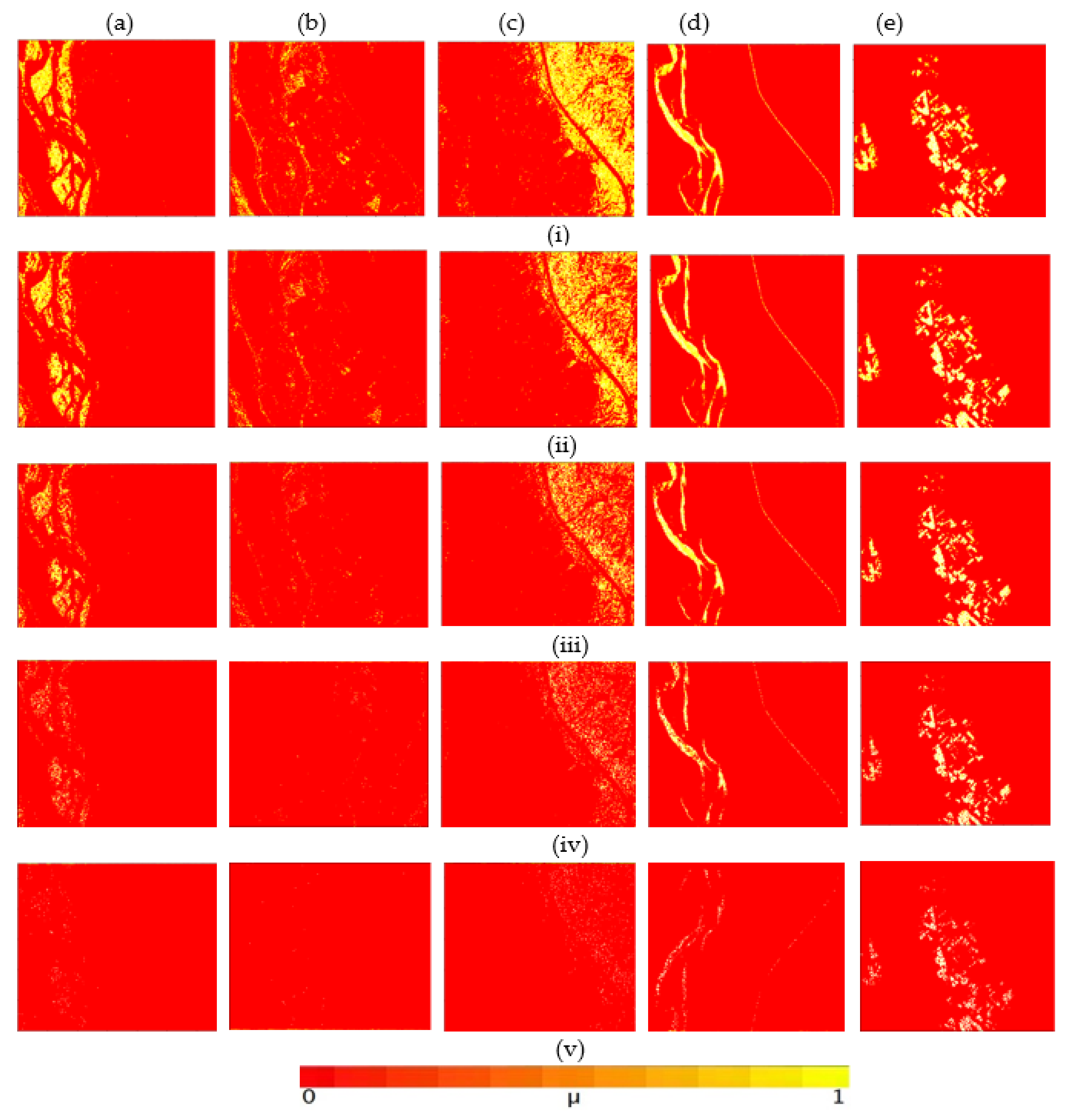
The α-cut FCM algorithm was implemented on the results obtained by using Cosine measure with m equals to 2.7. The generated fractional images of the α-cut FCM algorithm has been shown in Figure 7 for each α-cut starting from 0.5 to 0.9 with an interval of 0.1 for Formosat-2 data.

The membership grade of all the pixels in these fractional images ranges from 0 to 1. These fractional images were used as the reference data for measuring the accuracy of the results obtained from the Landsat-8 image. From the images in Figure 8, it has been observed that as the α-cut value was increased from 0.5 towards 0.9 with an interval of 0.1, the membership grades of the pixels which were less than the threshold value were removed. The yellow coloured pixels are the pure pixels for each class in response to the α-cut value and the red pixels show other classes with respect to the particular class in question. Similarly, fractional images have been obtained for Landsat-8 images using Cosine measure at m* equals 2.5 for each α-cuts ranging from 0.5 to 0.9. The fractional images obtained from Formosat-2 datasets were used as the reference images for the accuracy assessment of the Landsat-8 images. Similar results were obtained for composite measures with m* equals 2.5 for both Formosat-2 and Landsat-8 datasets.

4.3. Accuracy Assessment

The FCM classifier was applied with a supervised approach for classification of Landsat-8 data. For this process, a total of 20 training pixels were carefully chosen from each of the land-cover classes. The training sites were selected at various locations spread well over the Landsat-8 image.

In the FCM classifier using the supervised approach, Cosine measure was considered, as the results in Table 2, Table 3 and Table 4 show that cosine measure was the best measures out of all the 12 measures considered for this study. The membership value of all the pixels in the fractional images was ranging from 0 to 1. In this study, mean-aggregation method was used to maintain the scale ratio of resolutions of the reference data and the assessed data. The accuracy was assessed by the fuzzy-based techniques like FERM and SCM. The method of mean-aggregation was also followed by FERM and SCM so that the referenced data and the assessed data are on the same scale [11,46]. As the referenced data and the assessed data were brought to the same scale, the following fuzzy accuracy operators like FERM and SCM were used to measure the accuracy of the fractional images of the Landsat-8 dataset. Five hundred sample points (pixels) (100 samples per class [47]) were selected randomly as the test sites to carry out the accuracy assessment. The fuzzy user’s accuracy, producer’s accuracy, kappa coefficient and overall accuracy were computed for all the fuzzy accuracy operators using the error matrices.

Table 8. Details of accuracy assessment for classification results of Landsat-8 data using a single measure.

Accuracy Assessment Operators	FERM	SCM
User’s Accuracy (%)
Riverine Sand	86.05	86.88 ± 3.77
Fallow Land	60.90	62.45 ± 5.52
Forest	81.23	82.35 ± 4.15
Water	81.72	82.87 ± 2.97
Wheat	63.75	65.22 ± 5.26
Producer’s Accuracy (%)
Riverine Sand	66.30	67.78 ± 5.39
Fallow Land	85.92	86.60 ± 2.50
Forest	80.14	81.18 ± 2.75
Water	50.86	53.50 ± 9.36
Wheat	77.41	78.72 ± 3.68
Overall Accuracy (%)	73.96	75.24 ± 4.72
Fuzzy Kappa value		0.68 ± 0.06

shows the detailed statistics of the accuracy assessment.

The two best measures obtained in the section were Euclidean and Cosine with an optimized fuzzifier value at m* equals 2.5. However, there was no significant change in the classified outputs while optimizing the value of the weighting constant (λ). Thus, the value of lambda was set at λ equals 0.5 (mean value of the range of λ [0.10, 0.90]) for the classification, which signifies the contribution of both the measures of an equal distribution of 50%.

Table 9. Details of accuracy assessment for classification results of Landsat-8 data using composite measure.

Accuracy Assessment Operators	FERM	SCM
User’s Accuracy (%)
Riverine Sand	66.67	68.24 ± 6.25
Fallow Land	44.84	46.26 ± 4.25
Forest	86.30	86.94 ± 2.59
Water	76.83	77.76 ± 1.68
Wheat	64.31	65.92 ± 5.29
Producer’s Accuracy (%)
Riverine Sand	68.08	69.67 ± 5.93
Fallow Land	77.72	78.51 ± 2.20
Forest	75.28	76.46 ± 3.35
Water	42.30	43.72 ± 5.17
Wheat	78.99	80.11 ± 2.99
Overall Accuracy (%)	68.57	69.80 ± 4.21
Fuzzy Kappa value		0.61 ± 0.06

shows the detailed statistics of the accuracy assessment for the composite measure.

4.4. Performance with Untrained Class

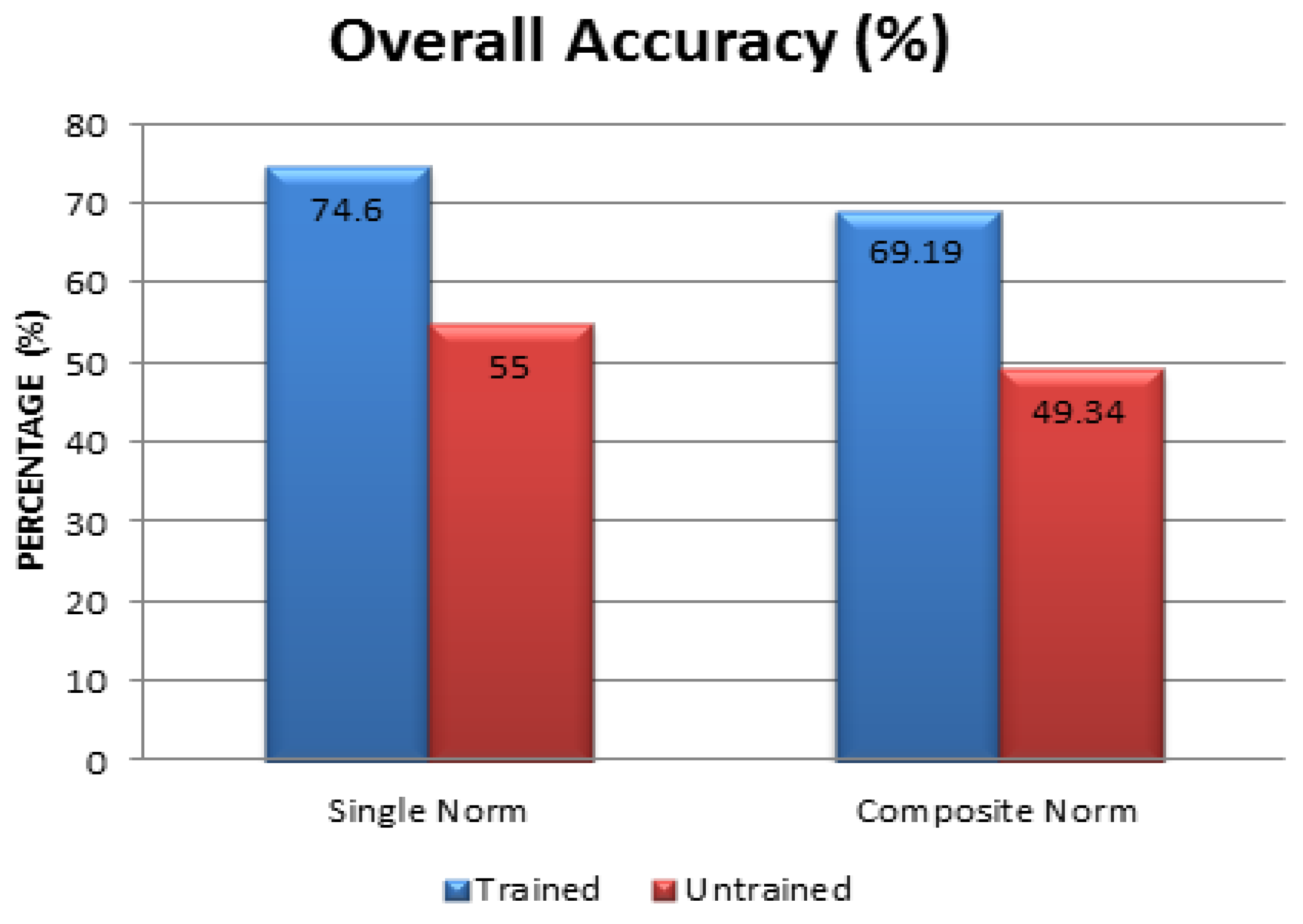
During the training stage of a classifier, some classes were ignored resulting in the untrained class. The untrained classes depict the higher degree of membership for classes which are spectrally different and hence, resulting in a drop in the accuracy of the classification [50]. In this work, for the developed FCM classifier, the mean values of wheat for Landsat-8 datasets were not considered for training. Figure 9 compares the overall accuracy results of both single measure as well as a composite measure for both trained and untrained cases, respectively. The results obtained after accuracy assessment in Figure 9 showed that the overall accuracy for trained classes was more than the untrained classes ranging from 49% to 55% for single and composite measures, respectively. These results showed that the removal of a class (wheat) for an untrained class reduced the overall accuracy; however, the trend was constant like in a trained dataset.

5. Discussion

In this study, single and composite, similarity or dissimilarity measures were integrated into the FCM objective function to handle mixed pixels in remote-sensing data. The main objective of this research was to study the behaviour of similarity and dissimilarity measures while handling the mixed pixels.

The foremost focus of this research work was on the optimization of different parameters for the different similarity and dissimilarity measures used in the FCM classifier. Setting optimal values for various parameters was necessary for their proper performance. Optimal values of m were achieved on the basis of the working of the particular measure while handling the pure and mixed pixels. For, FCM using single measures and FCM using composite measures the optimization of the fuzzifier (m*) was computed within the range from 1.1 to 3.0. On the basis of the statistics from Table 2, Table 3 and Table 4, the Cosine measure was found to be the best among all the measures with an optimized m* value of 2.7 for Formosat-2 data and m* value of 2.5 for Landsat-8 dataset. The composite measure was formed by using the two best measures (Euclidean measure and Cosine measure). The optimized value of m* for the composite measure was at 2.5 for both the Formosat-2 dataset and Landsat-8 dataset.

FCM classification has resulted in an overall accuracy (using SCM operator) of 75.24% and 69.80% for the Landsat-8 image with the Formosat-2 image as the referenced image while using single measure and composite measure, respectively. The average user’s accuracy using the same operator for the Landsat-8 image for single and composite measures were 75.95% and 69.02%, respectively, and the average producer’s accuracy were 73.56% and 69.69%, respectively. From these results, it was evident that there was an overall decline in the accuracy while using composite measures instead of a single measure. The usage of weighted composite measures was shown by [51], however, the results were unsatisfactory. The performance of the composite measures depends on the type of single measures taken into account as a combination. Taking two best measures in a combination would give a deterioration in the results with respect to single best measures, due to the weighting component.

The classification was tested on the various α-cut values starting from 0.5 to 0.9 with an interval of 0.1 with both single measure and composite measures with m* value of 2.5 and 2.7. The range of α-cut was chosen from 0.5 to 0.9 because the FCM clustering algorithm is sensitive to noise and thus the FCM clustering outputs do not show any result with a membership value of 1 [23]. When a suitable value of α-cut was chosen, noise and outliers would be outside the cluster cores as α-cut was a threshold value and any pixel with a membership value less than the threshold would not be considered. That is the reason we obtain either a very high accuracy or an accuracy of zero, as the α-cut value was moved towards 0.9. The concept of α-cut was used to remove noisy points. For example, if the α-cut value was set at 0.6 in the developed FCM algorithm, then the pixels having membership value greater than or equal to 0.6 would belong to the cluster core such that all the membership values of these pixels would become 1 for that concerned cluster and zero for the remaining clusters. However, if the pixels had membership value below 0.6, then the membership of the pixels remains the same. As the pixels had a small membership value for the cluster, these pixels would be considered as noise. Hence, these points were removed from that cluster. Figure 8 shows the clusters of the classes without the noisy pixels namely riverine sand, fallow land, forest, water and wheat at different α-cut values of 0.5, 0.6, 0.7, 0.8 and 0.9, respectively, for single measures incorporated in the FCM algorithm.

The classification was also verified on untrained classes where the FCM classifier was not trained about a class (in this study, wheat was untrained). There is an overall decrease in the accuracy in the untrained case in comparison with the trained case. The average overall accuracies for the single measure in case of trained and untrained were 74.6% and 55%, respectively, and for composite measures 69.19% and 49.34%, respectively. However, Figure 9 showed the overall trend of the accuracy was the same for both trained and untrained with respect to single and composite measures, respectively. This trend also explained that the incapability of FCM classifier to handle noise properly. On the removal of a class from the training samples, there was a fall in the accuracy of nearly 20% in both single and composite measures. This showed that for the classification, the class (wheat) removed was noise for the other classes in the training samples, hence, there was a dip in the overall accuracy from trained case to untrained case.

By considering the overall accuracy of the classification (Table 8 and Table 9), it can be established that FCM with the single measure (Cosine) performs better in classification than FCM with composite measures. FCM with α-cut also reduces the noise in the classified images (Figure 8), which helps in the handling of the mixed pixel problem in a better way. In this study, all the similarity and dissimilarity measures were evaluated for images of both medium and coarser resolutions. However, the behaviour of the measures may differ with different datasets and these similarity or dissimilarity measures may also be evaluated with a large number of various datasets to get a robust conclusion. It was stated by [49,52] that FCM with Euclidean measure performs better than diagonal Mahalanobis and Mahalanobis measures, but in this study it was found that Cosine measure outperforms the Euclidean measure.

6. Conclusions and Recommendation

The occurrence of mixed pixels in the remote-sensing images is largely due to the mismatch of the resolution of the images with respect to class size. Due to the presence of mixed pixels, there are chances of having an inaccuracy in the results obtained after classification. Sub-pixel classification using fuzzy based classifiers such as FCM are a solution to this kind of uncertainty in data. Thus, to solve the problem of mixed pixels, a fuzzy-based approach using different similarity and dissimilarity measures have been studied in this research work. The main objective of this research work was to study the behaviour of similarity and dissimilarity measures with FCM while handling the mixed pixels. The comparative study of different measures used, Cosine measure with m* value of 2.7, attained the highest overall accuracy during the classification. It was also witnessed that optimization of parameters like weighted constant (m*) and weighted component λ played a major role in the overall performance of the FCM-based classifier.

Various accuracy assessment methods are available to measure the accuracy of the classification. FERM and SCM have been recommended for the measurement of accuracy. The Landsat-8 image of the coarser resolution was assessed with a Formosat-2 image of finer resolution. The overall accuracy was low for the image of coarser resolution. This may be due to the lack of adjacency of the information in the coarser image with respect to the ground truth information.

Among the different similarity and dissimilarity measures, Cosine and Euclidean measures have given the best overall performance. These two measures were combined to form a composite measure with λ value equals to 0.5 and m* value of 2.5. The composite measure has lower overall accuracy in comparison with the single measure (Table 8 and Table 9). The performance of the composite measure depends on the individual performance of single measures selected to combine and form the composite measure. If the best single measure with higher performance is pooled with a measure having lower performance, the resultant measure will also have lower performance.

The concept of α-cut has also been incorporated into the FCM function to minimize the effect of noise in the FCM classifier. This has been done due to the incapability of FCM to handle the noise properly [23]. In this study, the effect of an untrained class on the accuracy of the classification was also carried out by dropping wheat as an untrained class, which resulted in a decrease in the overall accuracy in comparison to the trained case. To conclude, the FCM classifier with Cosine measure performed better than the conventional Euclidean measure. However, due to the incapability of the FCM classifier to handle noise properly, the classification accuracy was around 75%.

This study leads to some further works which can be implemented. First, the performance of the developed α-cut FCM classifier with different similarity and dissimilarity measures can be tested for a large heterogeneous area with high complexity in the land cover. Second, the performance of the α-cut in the FCM classifier can be proposed further for handling the noise in FCM, as it can form cluster cores with a membership grade close to 1, unlike the FCM clustering algorithm. Third, the results obtained for the single norm in this research also gives an opportunity to further study other fuzzy-based classification techniques which use the similarity or dissimilarity measures like the possibilistic c-means (PCM) classifier and other methods that handle uncertainty like multi-label classification, cellular automata, artificial neural networks and others. The accuracy tools, as well as the mode of generating the soft reference data for accuracy assessment for soft classifiers, are actively studied in the field of digital image processing. Instead of a supervised FCM approach, this study can be tested with unsupervised FCM classification. The next challenge will be to adapt this method to considerable general and comprehensive data.

References

- Tso, B.; Mather, P.M. Classification Methods for Remotely Sensed Data; CRC Press Taylor & Francis: London, UK; New York, NY, USA, 2001. [Google Scholar]
- Tyagi, U.; Kumar, A. Similarity and Dissimilarity Measures with Fuzzy Classifiers: SMIC Tool. In Proceedings of the 9th International Conference on ASEICT, New Delhi, India, 20–21 June 2015; Volume 2, p. 6. [Google Scholar]
- Harikumar, A. Effect of Discontinuity Adaptive MRF Models with Noise Classifier. Master’s Thesis, University of Twente, Enschede, The Netherlands, 2014; p. 126. [Google Scholar]
- Mukhopadhaya, S. Exploring Measures of Similarity and Dissimilarity for Fuzzy Classifier: From Data Quality to Distance Quality. Master’s Thesis, University of Twente, Enschede, The Netherlands, 2016; p. 99. [Google Scholar]
- Foody, G.M.; Arora, M.K. An evaluation of some factors affecting the accuracy of classification by an artificial neural network. Int. J. Remote Sens. 1997, 18, 799–810. [Google Scholar] [CrossRef]
- Stehman, S.V. Selecting and interpreting measures of thematic classification accuracy. Remote Sens. Environ. 1997, 62, 77–89. [Google Scholar] [CrossRef]
- Thomas, L.; Kiefer, R.W.; Chipman, J. Remote Sensing and Image Interpretation; John Wiley & Sons: Hoboken, NJ, USA, 2014. [Google Scholar]
- Foody, G.M. The Role of Soft Classification Techniques in the Refinement of Estimates of Ground Control Point Location. Am. Soc. Photogramm. Remote Sens. 2002, 68, 897–903. [Google Scholar]
- Kumar, A.; Ghosh, S.K.; Dadhwal, V.K. A Comparison of the Performance of Fuzzy Algorithm versus Statistical Algorithm Based Sub-Pixel Classifier for Remote Sensing Data. In Proceedings of the Mid-Term Symposium (ISPRS), Enschede, The Netherlands, 8–11 May 2006. [Google Scholar]
- Zadeh, L.A. Fuzzy Sets. Inf. Control 1965, 8, 338–353. [Google Scholar] [CrossRef]
- Binaghi, E.; Brivio, P.A.; Ghezzi, P.; Rampini, A. A fuzzy set-based accuracy assessment of soft classification. Pattern Recognit. Lett. 1999, 20, 935–948. [Google Scholar] [CrossRef]
- Stein, A. Fuzzy Methods in Image Mining. In Methods for Handling Imperfect Spatial Information; Jeansoulin, R., Papini, O., Prade, H., Schockaert, S., Eds.; Springer: Berlin/Heidelberg, Germany, 2010; Volume 256, pp. 243–268. [Google Scholar]
- Bezdek, J.C.; Ehrlich, R.; Full, W. FCM: The fuzzy c-means clustering algorithm. Comput. Geosci. 1984, 10, 191–203. [Google Scholar] [CrossRef]
- Kumar, A.; Ghosh, S.K.; Dhadhwal, V.K. Sub-pixel land cover mapping: SMIC system. In Proceedings of the ISPRS International Symposium on Geospatial Databases for Sustainable Development, Goa, India, 27–30 September 2006. [Google Scholar]
- Lopatka, J.; Pedzisz, M. Automatic modulation classification using statistical moments and a fuzzy classifier. In Proceedings of the WCCC-ICSP, 5th International Conference, Beijing, China, 21–25 August 2000; Volume 3, pp. 1500–1506. [Google Scholar]
- Besag, J. On the Statistical Analysis of Dirty Pictures. J. R. Stat. Soc. Ser. B Methodol. 1986, 48, 259–302. [Google Scholar] [CrossRef]
- Dilo, A. Representation of and Reasoning with Vagueness in Spatial Information: A System for Handling Vague Objects; ITC: Enschede, The Netherlands, 2006. [Google Scholar]
- Mukhopadhaya, S. Land use and Land Cover Change Modelling using CA-Markov Case Study: Deforestation Analysis of Doon Valley. J. Agroecol. Nat. Resour. Manag. 2016, 3, 1–5. [Google Scholar]
- Goshtasby, A. Image Registration: Principles, Tools and Methods; Springer: London, UK, 2012. [Google Scholar]
- Dunn, J.C. A Fuzzy Relative of the ISODATA Process and Its Use in Detecting Compact Well-Separated Clusters. J. Cybern. 1973, 3, 32–57. [Google Scholar] [CrossRef]
- Dwivedi, R.; Kumar, A.; Ghosh, S.K. Study of Fuzzy based Classifier Parameter across Spatial Resolution. Int. J. Comput. Appl. 2012, 50, 17–24. [Google Scholar] [CrossRef]
- Buckley, J.J.; Eslami, E. An Introduction to Fuzzy Logic and Fuzzy Sets; Physica-Verlag HD: Heidelberg, Germany, 2002. [Google Scholar]
- Yang, M.; Wu, K.; Hsieh, J.; Yu, J. A-Cut Implemented Fuzzy Clustering Algorithms and Switching Regressions. IEEE Trans. Syst. Man Cybern. Part B Cybern. 2008, 38, 588–603. [Google Scholar] [CrossRef] [PubMed]
- Byju, A.P. Non-Linear Separation of Classes Using a Kernel Based Fuzzy c-Means (KFCM) Approach. Master’s Thesis, University of Twente, Enschede, The Netherlands, 2015. [Google Scholar]
- Theodoridis, S.; Koutroumbas, K. Clustering: Basic Concepts. In Pattern Recognition, 4th ed.; Academic Press: Cambridge, MA, USA, 2009; pp. 595–625. [Google Scholar]
- Guyon, I. Pattern classification. Pattern Anal. Appl. 1998, 1, 142–143. [Google Scholar] [CrossRef]
- Hasnat, A.; Halder, S.; Bhattacharjee, D.; Nasipuri, M.; Basu, D.K. Comparative Study of Distance Metrics for Finding Skin Color Similarity of Two Color Facial Images; ACER: New Taipei City, Taiwan, 2013; pp. 99–108. [Google Scholar]
- Bray, J.R.; Curtis, J.T. An Ordination of the Upland Forest Communities of Southern Wisconsin. Ecol. Monogr. 1957, 27, 325–349. [Google Scholar] [CrossRef]
- Shyam, R.; Singh, Y.N. Face recognition using augmented local binary pattern and Bray Curtis dissimilarity metric. In Proceedings of the 2015 2nd International Conference on Signal Processing and Integrated Networks (SPIN), Noida, India, 19–20 February 2015; pp. 779–784. [Google Scholar]
- Van der Heijden, F.; Duin, R.P.W.; de Ridder, D.; Tax, D.M.J. Classification, Parameter Estimation and State Estimation: An Engineering Approach Using MATLAB; Wiley: Hoboken, NJ, USA, 2004. [Google Scholar]
- Balu, R.; Devi, T. Design and Development of Automatic Appendicitis Detection System using Sonographic Image Mining. Int. J. Eng. Innov. Technol. 2012, 1, 2277–3754. [Google Scholar]
- Lance, G.N.; Williams, W.T. Computer Programs for Hierarchical Polythetic Classification (‘Similarity Analyses’). Comput. J. 1996, 9, 60–64. [Google Scholar] [CrossRef]
- Jurman, G.; Riccadonna, S.; Visintainer, R.; Furlanello, C. Canberra Distance on Ranked Lists. In Proceedings of the Advances in Ranking NIPS 09 Workshop, Vancouver, BC, Canada, 7–9 December 2009; pp. 22–27. [Google Scholar]
- Emran, S.M.; Ye, N. Robustness of Canberra Metric in Computer Intrusion Detection. In Proceedings of the 2001 IEEE Workshop on Information Assurance and Security United States Military Academy, West Point, NY, USA, 5–6 June 2001; pp. 80–84. [Google Scholar]
- Vassiliadis, S.; Hakkennes, E.A.; Wong, J.S.S.M.; Pechanek, G.G. The sum-absolute-difference motion estimation accelerator. In Proceedings of the 24th Euromicro Conference, Vasteras, Sweden, 27 August 1998; Volume 2, pp. 559–566. [Google Scholar]
- Sari, S.; Roslan, H.; Shimamura, T. Noise Estimation by Utilizing Mean Deviation of Smooth Region in Noisy Image. In Proceedings of the Fourth International Conference on Computational Intelligence, Modelling and Simulation, Kuantan, Malaysia, 25–27 September 2012; pp. 232–236. [Google Scholar]
- Scollar, I.; Weidner, B.; Huang, A.T.S. Image Enhancement Using the Median and the Interquartile Distance. Comput. Vis. Graph. Image Process. 1984, 25, 236–251. [Google Scholar] [CrossRef]
- Zehavi, E. 8-PSK Trellis Codes for a Rayleigh Channel. IEEE Trans. Commun. 1992, 40, 873–884. [Google Scholar] [CrossRef]
- Singhal, A. Modern Information Retrieval: A Brief Overview. Data Eng. Bull. 2001, 24, 35–43. [Google Scholar]
- Tan, P.-N.; Steinbach, M.; Kumar, V. Modern Information Retrieval: A Brief Overview. In Introduction to Data Mining, 2nd ed.; Addison-Wesley Longman Publishing Co., Inc.: Boston, MA, USA, 2006. [Google Scholar]
- Ye, J. Multicriteria decision-making method based on a cosine similarity measure between trapezoidal fuzzy numbers. Int. J. Eng. 2011, 3, 7. [Google Scholar] [CrossRef]
- Song, S.; Zhu, H.; Chen, L. Probabilistic correlation-based similarity measure on text records. Inf. Sci. 2014, 289, 8–24. [Google Scholar] [CrossRef]
- Zhang, M.; Therneau, T.; McKenzie, M.A.; Li, P.; Yang, P. A fuzzy c-means algorithm using a correlation metrics and gene ontology. Nat. Med. 2008, 6–9. [Google Scholar] [CrossRef]
- Mahalanobis, P.C. On The Generalized Distance in Statistics. Proc. Natl. Inst. Sci. India 1936, 2, 49–55. [Google Scholar]
- Okeke, F.; Karnieli, A. Methods for fuzzy classification and accuracy assessment of historical aerial photographs for vegetation change analyses. Part I: Algorithm development. Int. J. Remote Sens. 2006, 27, 153–176. [Google Scholar] [CrossRef]
- Silván-Cárdenas, J.L.; Wang, L. Sub-pixel confusion–uncertainty matrix for assessing soft classifications. Remote Sens. Environ. 2008, 112, 1081–1095. [Google Scholar] [CrossRef]
- Congalton, R.G. A review of assessing the accuracy of classifications of remotely sensed data. Remote Sens. Environ. 1991, 37, 35–46. [Google Scholar] [CrossRef]
- Pontius, R.G.; Cheuk, M.L. A generalized cross-tabulation matrix to compare soft-classified maps at multiple resolutions. Int. J. Geogr. Inf. Sci. 2006, 20, 1–30. [Google Scholar] [CrossRef]
- Kumar, A.; Ghosh, S.K.; Dadhwal, V.K. Full fuzzy land cover mapping using remote sensing data based on fuzzy c -means and density estimation. Can. J. Remote Sens. 2007, 33, 81–87. [Google Scholar] [CrossRef]
- Foody, G.M. Estimation of sub-pixel land cover composition in the presence of untrained classes. Comput. Geosci. 2000, 26, 469–478. [Google Scholar] [CrossRef] [Green Version]
- Izakian, H.; Pedrycz, W. Agreement-based fuzzy C-means for clustering data with blocks of features. Neurocomputing 2014, 127, 266–280. [Google Scholar] [CrossRef]
- Dutta, A. Fuzzy c- Means Classification of Multispectral Data Incorporating Spatial Contextual Information by Using Markov Random Field. Master’s Thesis, University of Twente, Enschede, The Netherlands, 2009. [Google Scholar]
Figure 1.
Research methodology.
Figure 2.
Flow chart for optimizing the parameter.
Figure 3.
Infrared image is of Haridwar area, Uttarakhand, India showing the different land-use classes.
Figure 4.
Details of simulated images.
Figure 5.
The result of simulated image using Cosine measure with m* equals to 2.7.
Figure 6.
The result of real image using Cosine measure with m* equals 2.7.
Figure 7.
The misclassified outputs in red circles while using composite measure with Euclidean and Cosine measures at m* equal to 2.5 and λ equals to 0.5.
Figure 8.
Generated fractional images for cosine measure at optimized m* value of 2.7 of Formosat-2 data for (i) α-cut = 0.5 (ii) α-cut = 0.6 (iii) α-cut = 0.7 (iv) α-cut = 0.8 (v) α-cut = 0.9 for all the classes (a) riverine sand (b) fallow land (c) forest (d) water (e) wheat.
Figure 9.
Details of accuracy assessment in trained and untrained case of classification results for Landsat-8 data with single and composite measure respectively.