Confronting Soil Moisture Dynamics from the ORCHIDEE Land Surface Model With the ESA-CCI Product: Perspectives for Data Assimilation

Abstract

Soil moisture plays a key role in water, carbon and energy exchanges between the land surface and the atmosphere. Therefore, a better representation of this variable in the Land-Surface Models (LSMs) used in climate modelling could significantly reduce the uncertainties associated with future climate predictions. In this study, the ESA-CCI soil moisture (SM) combined product (v4.2) has been confronted to the simulated top-first layers/cms of the ORCHIDEE LSM (the continental part of the IPSL Earth System Model) for the years 2008-2016, to evaluate its potential to improve the model using data assimilation techniques. The ESA-CCI data are first rescaled to match the climatology of the model and the signal representative depth is selected. Results are found to be relatively consistent over the first 20 cm of the model. Strong correlations found between the model and the ESA-CCI product show that ORCHIDEE can adequately reproduce the observed SM dynamics. As well as considering two different atmospheric forcings to drive the model, we consider two different model parameterizations related to the soil resistance to evaporation. The correlation metric is shown to be more sensitive to the choice of meteorological forcing than to the choice of model parameterization. Therefore, the metric is not optimal in highlighting structural deficiencies in the model. In contrast, the temporal autocorrelation metric is shown to be more sensitive to this model parameterization, making the metric a potential candidate for future data assimilation experiments.

1. Introduction

Land-surface models (LSMs) are crucial components of climate models, representing the matter and energy transfers at the continental interface with the atmosphere. They therefore play a key role on the climate model simulations, past, present, and future predictions. Within LSMs, surface soil moisture (SM) heavily influences the hydrological interactions between soil, vegetation, and atmosphere. Because of the coupling between water and carbon cycles at the leaf and soil levels, it is a major constraint for the assimilation of carbon by the vegetation through photosynthesis [1], whose net global value is still largely debated [2,3,4]. Moreover, SM governs the partition between runoff and infiltration and is thus a key element of the global water cycle. Consequently, correctly representing this variable in LSMs could highly improve both short- and long-term forecasts [5,6,7,8,9].

Despite considerable improvements in recent years, estimated water and carbon fluxes in LSMs are still affected with biases and large uncertainties. Three different sources of uncertainty prevail in LSMs: the external forcing, model structure and its parameterization. More specifically, simulated SM exhibit large sensitivities to meteorological forcing data and to land-surface parameterizations [10]. Since SM variability is largely driven by precipitation, the meteorological forcing data used to run the LSM could have a greater weight on the comparison scores than the parameterization of the model itself [11].

Simulated SM depends on the model version and configuration used. Since it is impossible to accurately model and represent all the land-surface processes in an LSM due to lack of knowledge and computing limitations, choices are made to determine which processes are included and how they are described in the model. These choices contribute to the structure of the model. For example, how one chooses to discretize the upper soil layers will affect the soil moisture dynamics [12], similarly the inclusion of a soil resistance term for water transfer will greatly affect evapotranspiration. It is important to separate the different sources of errors to understand whether the deficiencies in the model process are due to the forcing used or the model structure and configuration. To improve the representation of a variable such as SM in LSMs, the model can be confronted with the observations. These observations can be measured in situ, i.e., locally, or remotely, for example, from space instruments. Since soil moisture is difficult to observe at large scales due to its high spatial and temporal variability, satellite data can provide much needed consistent and comparable global datasets. Extra care needs to be taken with SM data since it is not directly observed but rather estimated using backscattering signals and brightness temperatures through different inversion algorithms.

Over the last decade, the quality and quantity of the Earth Observations has vastly improved and has been used to evaluate the performance of LSMs over different climatology and hydrological environments. For example, GRACE (Gravity Recovery and Climate Experiment) data has been used to evaluate land water storage in several LSMs (e.g., ORCHIDEE; [13]). GRACE has been used to evaluate the CLM (Community Land Model) over Africa, specifically to assess a soil resistance parameterization in the model [14]. Ref. [15] evaluate the CLM and GLDAS models over Africa using GRACE and other remote sensing data to highlight discrepancies between the models’ evapotranspiration outputs. Other remote sensing products used to evaluate the representation of soil moisture in LSMs include SMOS (Soil Moisture and Ocean Salinity, [16]), SMAP (Soil Moisture Active Passive, [17]) and ASCAT (Advanced Scatterometer, [18]). These have been used to evaluate LSMs over a wide range of climatologies e.g., [19] consider ASCAT and SMOS over Europe and Northern Africa, and [20] use SMAP assess storm event runoff over America. Satellite retrievals have also allowed global comparison (e.g., [21]). Of course, there are several other remote-sensed products used to evaluate LSMs, such as biomass, albedo and NDVI (normalized difference vegetation index); however, these are beyond the scope of this study.

As well as evaluating LSMs, satellite retrieval can be used to improve models through data assimilation (DA). Several recent studies have used data DA to improve the representation of SM in LSMs, by either optimizing initial conditions or the model parameters e.g., [22,23,24,25,26,27], and therefore improve LSMs ability to forecast events such as droughts and floods e.g., [23,24,26,28]. SM data can also be used to improve other components of the LSM such as the carbon cycle [29]. Furthermore, DA can be used to reveal structural errors in the model [30,31]. However, before attempting to improve the model through DA, a thorough comparison of the observations with the model output is needed. Such a comparison allows us to assess whether the physical properties in both the observations and model output are comparable, and to select which model configuration and forcing to use at a later stage. This allows to evaluate whether the model is sophisticated enough and whether the observations can improve the model through assimilation or not. It then helps determining the most appropriate metrics to use in an objective function to be optimized which will depend on the aspect of the model under focus. In addition, most DA methods rely on Gaussian statistics. Therefore, a proper assessment of the satellite and model errors is needed, with potential bias correction, before any assimilation step.

The ESA-CCI multi-instruments dataset provides the SM observations used in this study. Thanks to its large spatio-temporal coverage, the ESA-CCI product offers a good opportunity to benchmark LSMs and improve their parametrization with DA techniques [32]. Combining several products from a broad range of instruments allows to get a large spatio-temporal coverage, which is suitable for global LSMs evaluations, and provides additional information at these larger scales compared to in situ observations in a global assimilation process. Moreover, active and passive instruments have been found to complement each other as they are affected differently by vegetation density (active instruments perform better over moderate vegetation areas whereas passive instruments give more reliable estimates over arid regions) and radio frequency interference contamination which alters L-band instruments measures [21]. The SMOPS soil moisture product [33] is another example of a blended soil moisture data set; however, this product does not cover as many years as the ESA-CCI product.

There are some known errors linked to the satellite data themselves which need to be considered (see [32]). For example, the observations can be spatially inhomogeneous due to the satellite’s retrieval heavy dependence on surface and sub-surface properties such as soil texture and vegetation. Similarly, the satellite data suffer from temporal inhomogeneity because of instrument drift and lifespan issues. The sampling of the observations is not continuous and in the case of the ESA-CCI SM product where each independent dataset has been rescaled to be merged together, combining different instruments from different periods adds temporal inhomogeneity to the final dataset and thus complications for model evaluations.

The quality of the ESA-CCI SM product has already been evaluated on a global scale by several studies with encouraging results. The merging of active and passive products has been shown to increase the number of observations and hence coverage, while keeping the same relative dynamics and minimally changing the accuracy [23,32,34,35]. By comparing the blended product to reanalysis and in situ measurements, [36] found that the product was able to capture the annual cycle of SM and its short-term variability. The quality of the product has been shown to increase with time due to the addition of new satellites and methods use to merge them [32]. A comprehensive list of studies using the ESA-CCI SM product can be found in [32].

In this study, the ESA-CCI SM product is compared with the process-based global LSM ORCHIDEE (ORganizing Carbon and Hydrology In Dynamic EcosystEm, [37]) at the global scale. ORCHIDEE has been recently endowed with a new 11 layers hydrological model which allows to refine the representation of soil water transfers. This discretization scheme offers a unique opportunity to match as closely as possible the representative depth of the satellite instrument products. While the paper focuses on a comparison of the soil moisture dynamics simulated by ORCHIDEE land-surface model with ESA-CCI soil moisture product, the analysis is done with a future data assimilation experiment in mind. Even though no data assimilation is performed in this work, this paper serves as an important preliminary study assessing the following more specific objectives:

• How should the satellite product be processed (bias corrected) for a meaningful comparison with the ORCHIDEE LSM?
• What are the impacts of the selected model representative soil depth and the meteorological forcing on the comparison between the satellite and model SSM?
• What are the strengths and weaknesses of a few (widely used) temporal comparison metrics? What is the potential of these metrics for future model structure/parameter optimization?

2. Methods and Data

2.1. The ORCHIDEE Land-Surface Model

The ORCHIDEE LSM [37] allows the representation as explicit as possible of processes governing water, carbon, and energy budgets of the terrestrial biosphere. It has a high spatial resolution flexibility (based on the meteorological forcing spatial resolution) and a temporal resolution of 30 min. ORCHIDEE conceptually includes (i) a Soil Vegetation Atmosphere Transfer (SVAT) scheme, which calculates energy, water and carbon fluxes between soil, plant and atmosphere; (ii) a module describing carbon flow within ecosystems (plants and soils) and (iii) a sub-model describing the long-term dynamics of vegetation which is not activated in this study. We use the main version of ORCHIDEE (Trunk, revision 4783) that corresponds to the version used in the IPSL earth system model for the ongoing CMIP6 (Coupled Model Intercomparison Project Phase 6) climate simulations. This version has recently been improved with a multi-layer hydrological model which should be ideally suited to confront remotely sensed and simulated soil moisture products, thanks to its high vertical resolution [38,39,40]. In this new scheme, hydrology is resolved using the Richards equation over the first 2 m of soil with an 11-layer discretization. Increasing grid spacing is used throughout the soil column, allowing a finer discretization at the top of the column (

Table 1. Table showing the depths of the 11-layer discretization based on work by [39] and adapted from [41].

Layer	Layer Thickness (m)	Integrated Depth (m)
1	0.001	0.001
2	0.003	0.004
3	0.006	0.010
4	0.012	0.022
5	0.023	0.045
6	0.047	0.092
7	0.092	0.186
8	0.188	0.374
9	0.375	0.750
10	0.750	1.500
11	0.500	2.000

). The Richards equation describes the diffusion of water according to the soil properties (prescribed following a global texture map). The SM at different levels is thus computed at each time step as influenced by rain infiltration, evaporation, transpiration, and drainage. For the bottom boundary condition, three options are possible: 1- free drainage (under the hypothesis that hydraulic head is constant beneath the last layer), 2- no drainage and 3- a mixed option between the two previous ones. Free drainage is used as default. Concerning the upper boundary condition, bare soil evaporation in ORCHIDEE is the minimum between potential evaporation and the hydrological flux allowed by diffusion. Then, soil water infiltration is obtained by solving the Green-Ampt equation which represents the evolution of the wetting front through the different soil layers.

In ORCHIDEE, vegetation is represented by 15 plant functional types (PFTs). To define soil properties, these PFTs are aggregated into 3 groups classified as bare soil, low vegetation (grasses and crops) and high vegetation (forests). This allows to divide each grid box into 3 tiles for which an independent hydric budget is calculated, by using the 11-layer physically based hydrology scheme. In the analysis presented here only the grid box weighted average SM profile (based on the fraction of vegetation) is considered.

2.2. ESA-CCI SM Product

The ESA-CCI SM project is part of the ESA (European Space Agency) Program on Global Monitoring of Essential Climate Variables (ECV), better known as the Climate Change Initiative (CCI) and initiated in 2010. A first version of the ESA-CCI SM product was released in June 2012 by the Vienna University of Technology [42]. In this study, we use the new version of the global ESA-CCI SM product (v4.2), released in January 2018 and freely available at http://esa-soilmoisture-cci.org/, that extends the data record from November 1978 to December 2016.

ESA-CCI SM is based on a series of active and passive microwave satellite sensors. Three datasets are provided: a merged passive-only (produced from multi-frequency radiometers), a merged active-only (produced from C-band scatterometers) and a combined active and passive SM product. In this new version, the exploited passive instruments are Scanning Multichannel Microwave Radiometer (SMMR), Special Sensor Microwave/Imager (SM/I), Tropical Rainfall Measuring Mission Microwave Imager (TMI), Advanced Microwave Scanning Radiometer for Earth Observation System (ASMR-E) and, added more recently, AMSR-2 and WindSat. The algorithm developed by the Vrije Universiteit Amsterdam in collaboration with the National Aeronautics and Space Administration (VUA-NASA) has been used to retrieve SM from remote-sensed measurements [43]. The active instruments exploited in this new version are the C-band scatterometers on board of the European Remote Sensing (ERS-1&2) and the Advanced SCATterometer (ASCAT). The change detection algorithm developed by the Vienna University of Technology (TU-Wien) has been applied here to retrieve SM from remote-sensed measurements [18,44]).

To provide a global coverage, the active and passive retrievals were combined. Since data provided by the retrievals have different units, to merge them, the SM values need to be rescaled into a common climatology. Therefore, data were scaled by GLDAS-Noah surface soil moisture product (v1, soil depth 10 cm) by a direct CDF-matching of the collocated observations [45]. The final combined ESA-CCI SM dataset is based on the spatial distribution of the temporal correlation between active-only and passive-only datasets. Over regions with correlation coefficients greater than 0.65, a simple average between active and passive measurements is used. Outside these regions, the merged passive-only dataset is used over areas with sparse vegetation density and the merged active-only dataset is used over areas with moderate vegetation density.

The ESA-CCI SM product provides daily SM, with a spatial resolution of 0.25 degrees, together with quality flags indicating the possible presence of dense vegetation, snow, or a temperature below $0{}^{\circ }$C. For our study, we used only the final combined dataset which is provided in volumetric units (m${}^3/$m${}^3$) and furnishes the largest spatio-temporal coverage of the three ESA-CCI SM datasets available.

2.3. Simulation Set Up

2.3.1. ORCHIDEE Configurations

In this study, the CMIP6 version of the ORCHIDEE model is run globally at a resolution of 0.5${}^{\circ }$. Using the half-hourly moisture content output, daily values of soil moisture are calculated using the weighted average of the 3 hydric budgets for soil columns associated with bare soil, forests, and grasslands PFTs. The distribution of PFTs and soil textures are determined according to some ancillary files created for CMIP6.

There is an option to account for a soil resistance term in ORCHIDEE which is used for the calculation of soil evaporation rates. Namely, it affects bare soil evaporation $E_g$ which is calculated using the following equation:

$$E_g=min(E_{\mathrm{pot}}/(1+r_{\mathrm{soil}}/r_a),Q)$$

(1)

where $E_{\mathrm{pot}}$ denotes the potential evaporation, $r_a$ denotes the aerodynamic resistance and Q is the supply of water by diffusion in the soil. When $r_{\mathrm{soil}}=0$, the resistance term disappears and $E_g$ is simply the minimum of the potential evaporation and the supply. The soil resistance term itself is calculated following the formulation of [46]

$$r_{\mathrm{soil}}=exp(8.2-4.3·W_1)$$

(2)

where $W_1$ is the wetness of the first 4 layers of the soil (2.2 cm) found by dividing the soil moisture in these layers by the corresponding moisture at saturation. Most of our analysis will be conducted over these first 4 layers of the model output. The coefficients in this equation have been determined in [46]’s study and are therefore specific to their model. These values may need to be reconsidered or indeed calibrated for the ORCHIDEE model later.

This soil resistance term is included by default in our simulations, with the exception of one comparative run where $r_{\mathrm{soil}}$ is set to zero.

2.3.2. Meteorological Forcing

We use two different meteorological forcings to drive ORCHIDEE in this study. The first is the CERASAT forcing data, used by default in our simulations. This is a 3-hourly climate reanalysis dataset spanning 8 years between 2008 and 2016 generated by ECMWF within the ERACLIM2 project. It has been produced specifically for the satellite era [47]. The second, used for a comparative run, is CRUNCEP, a 6-hourly 0.5${}^{\circ }$ global forcing product (1901–2015) which is a combination of the annually updated CRU-TS monthly climate dataset [48] and NCEP climate reanalysis [49]. Rainfall, cloudiness, relative humidity, and temperature are taken from the CRU while the other fields (pressure, longwave radiation, windspeed) were directly derived from NCEP. The forcings are interpolated to the half-hourly time step of the model.

In addition, Multi-Source Weighted-Ensemble Precipitation (MSWEP; [50]) data is used during the analysis step. The MSWEP data have a 0.25${}^{\circ }$ spatial resolution and a 3-hourly temporal resolution. This forcing is independent from the two datasets used to drive the ORCHIDEE model, as well as the forcing data used to generate the GLDAS reanalysis, used in scaling the ESA-CCI product.

2.3.3. Land Cover

ORCHIDEE uses land-cover maps to prescribe the distribution of vegetation used in the simulation. By default, we use the yearly land-cover maps created for the CMIP6 release of the model. These maps have been created through aggregation of the latest ESA-CCI land-cover map for 2010 (v2.0.7b) at 300 m resolution from 38 ESA land-cover classes into 15 ORCHIDEE PFTs at 0.5${}^{\circ }$ resolution [51,52]. For producing historical PFT maps (1860–2010) the resulting map has been further merged with the LUH2 dataset (Land-Use Harmonization, http://luh.umd.edu/). The overall protocol of the ORCHIDEE PFT maps production is outlined here: https://orchidas.lsce.ipsl.fr/dev/lccci/.

For our comparative run, an older version of the land-cover maps created for the CMIP5 LSM generation is used. These maps differ from the CMIP6 maps by the initial ESA-CCI land-cover map used (the epoch map for 2010 has been used, v1.6.1), and the protocol for merging the ESA data with LUH2 dataset has been slightly improved since that time.

2.3.4. Model Spin Up

The ORCHIDEE simulations include a spin up phase, that brought the prognostic variables including vegetation state and soil moisture content into equilibrium. The protocol follows that from the TRENDY model intercomparison (see http://dgvm.ceh.ac.uk/node/21/) with several hundred years of spin up, recycling the first 10 years of each meteorological forcing. Please note that such protocol includes a transient phase with increasing atmospheric CO${}_2$ concentration and changes in land cover, as it is primarily designed for the spin up of long-term soil carbon stock variables (not necessary for this paper). The spin up is followed by a historical simulation over the period of the ESA-CCI SM product.

2.3.5. Model Data Comparison

Both the model output and the observations used in the comparison were upscaled to the same spatial and temporal resolution (i.e., daily and global using a resolution of 0.5${}^{\circ }$), making it is possible to match up the time series at each grid point. The observed values with the quality flag indicating dense vegetation, snow, or freezing temperature were disregarded, as well as the modelled data corresponding to these points. Similarly, points are masked when the modelled surface temperature is less than $0{}^{\circ }$C, suggesting snow cover or frozen soil moisture values at that time and location.

Satellite SM observations represent only the top few centimeters of the soil column. From the eleven soil moisture layers simulated by ORCHIDEE (as described in Table 1), the first 4 layers spanning the top 2.2 cm of soil are most closely related to the instruments theoretical global mean sensing depth of 2 cm [32]. We thus choose this depth as the reference and averaged the model SM over the 4 top layers for the comparison. In addition, we also tested the impact of choosing different depths. The first 6 layers span the top 9.2 cm of the soil which is closer the GLDAS-Noah model depth simulation (the GLDAS-Noah model is used in combining the different products used to form ESA-CCI SM data). Additionally, the in situ data used in several studies to benchmark the satellite data is typically 5 cm which is closer to the integrated depth of 4.5 cm (layer 5). This raises the question of how to link observations to model variables and thus motivates the sensitivity analysis on the selected model depth, reported in Section 3.2.

2.3.6. Performed Simulations

The different simulations used in this study are outlined in

Table 2. The different simulations used in this study; differences from the reference run are in bold.

Simulation	Climate Forcing	Land Cover	Soil Resistance
ORC_REF	CERASAT	LC6	Y
ORC_CRU	CRUNCEP	LC6	Y
ORC_LC5	CERASAT	LC5	Y
ORC_NoRs	CERASAT	LC6	N

. Since CERASAT only covers 2008-2016, our analysis will focus on this period. This is also the period for which the ESA-CCI SM combined product provides close to a complete spatio-temporal coverage [32]. In this paper, we compare our default run (ORC_REF) to ORC_CRU in Section 3.4 to assess the effect of meteorological forcing data on simulated SM values. Also in Section 3.4, ORC_REF is compared to ORC_LC5 to evaluate the effects of different land-cover maps. ORC_REF is finally compared to ORC_NoRs in Section 3.7 to discuss the effect different parameterizations can have on modelled SM.

2.4. Data Processing and Statistical Analysis

All the metrics described in this section are calculated over the entire time period n and considered at every location i; $x_{i,t=1\dots n}$ and $y_{i,t=1\dots n}$ denote the time series of two datasets at that given location.

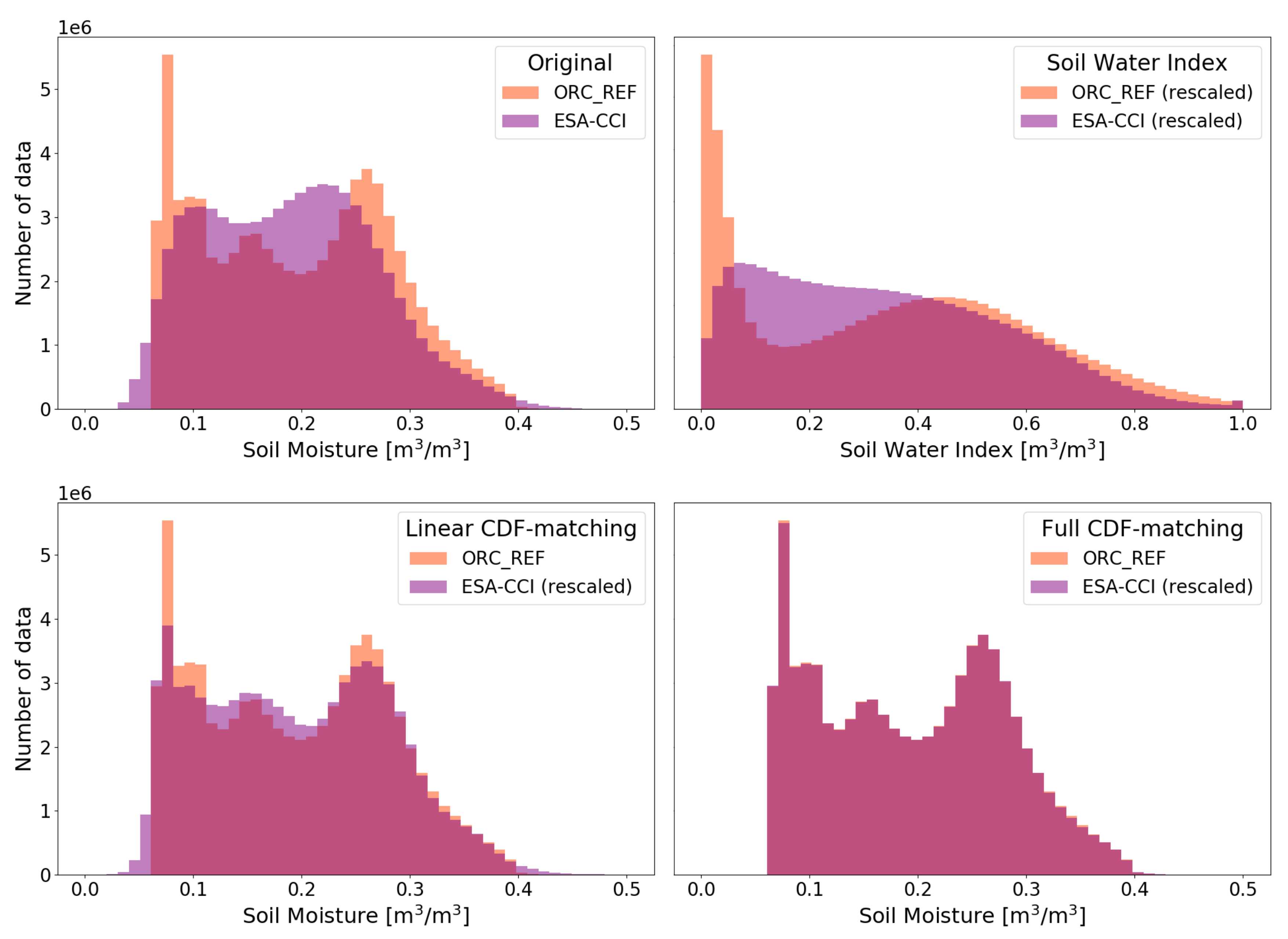
2.4.1. Statistically Rescaling and Bias Correcting the Observations

Cumulative density function (CDF)-matching schemes are used in this study to rescale the observed soil moisture y to the modelled soil moisture x (further explained in Section 3.1). Two CDF-matching algorithms are implemented [53]. The first is a linear CDF-matching which matches the mean and standard deviation in the following manner. Let $x_{i,t=1\dots n}$ and $y_{i,t=1\dots n}$ denote the time series of the two datasets for a given location i. Similarly, let ${\sigma }_{x_i}$ and ${\sigma }_{y_i}$ denote the standard deviation of each dataset respectively at location i. Then to obtain rescaled $y_{i,t}^{*}$ at each grid point, we use the following equation

$$y_{i,t}^{*}=\frac{{\sigma }_{x_i}(y_{i,t}-\overline{y_i})}{{\sigma }_{y_i}}+\overline{x_i}.$$

(3)

The second algorithm used a full CDF-matching which, in addition to the mean and standard deviation, matches higher moments of the distribution. The CDFs function of $y_i$ is matched to the CDF $y_i$ such that $y_i^{*}$ satisfies the following equation:

$${\mathrm{cdf}}_{x_i}\left(y_i^{*}\right)={\mathrm{cdf}}_{y_i}\left(y_i\right).$$

(4)

We use the python software (pytesmo package) to do this matching [54].

In another approach to rescale data, it is also normalized in the following manner:

$${\widehat{x}}_{i,t}=\frac{x_{i,t}-min{x}_i}{max{x}_i-min{x}_i}.$$

(5)

When applied to SM data, this normalization translates values to what is known as the Soil Water/Wetness Index (SWI).

2.4.2. Seasonal and Inter-Annual Variability

To separate seasonal effects from faster components, sub-monthly variations (also shown as monthly anomalies) are calculated. The raw data are divided into two components:

• a slow-varying component (SC) which represents seasonal variability. This is calculated in two steps. First, the mean annual cycle over the 8 years of data is calculated ($\overline{x_i^a}$). Then, following [55], the signal is averaged using a 35-day moving window. Considering a 35-day period $P=[t-17,t+17]$, a minimum of 5 values are needed to calculate the average soil moisture for this period resulting in the slow-varying component:

  $$x_{i,t}^{\mathrm{SC}}=\overline{\overline{x_i^a}\left(P\right)}.$$

  (6)
  When there are not 5 values within P for a given grid point, the grid point is then ignored for that given period.
• a fast-varying component (FC), or daily anomaly, given by:

  $$x_{i,t}^{\mathrm{FC}}=x_{i,t}-x_{i,t}^{\mathrm{SC}}.$$

  (7)

2.4.3. Correlation Scores

We use the Pearson product-moment correlation coefficient, r, to assess the relative agreement of the temporal structures between two datasets:

$$r=\frac{{\sum }_{t=1}^n(x_{i,t}-\overline{x_i})(y_{i,t}-\overline{y_i})}{\sqrt{{\sum }_{t=1}^n{(x_{i,t}-\overline{x_i})}^2}\sqrt{{\sum }_{t=1}^n{(y_{i,t}-\overline{y_i})}^2}}.$$

(8)

We also consider spatial correlations. These are calculated using same formula but on single vector of locations at each time step.

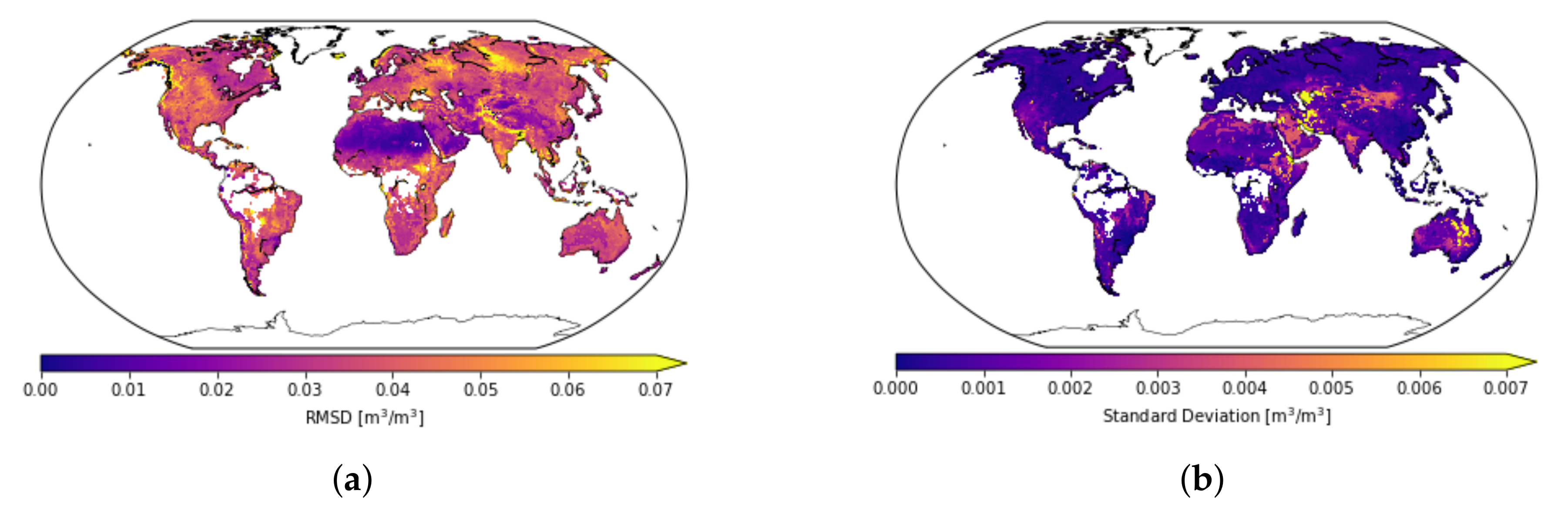
2.4.4. Root Mean Standard Deviation

To calculate the difference between two datasets, we used the root mean standard deviation (RMSD):

$$RMSD=\sqrt{\frac{{\sum }_{t=1}^n{(x_{i,t}-y_{i,t})}^2}{n}}.$$

(9)

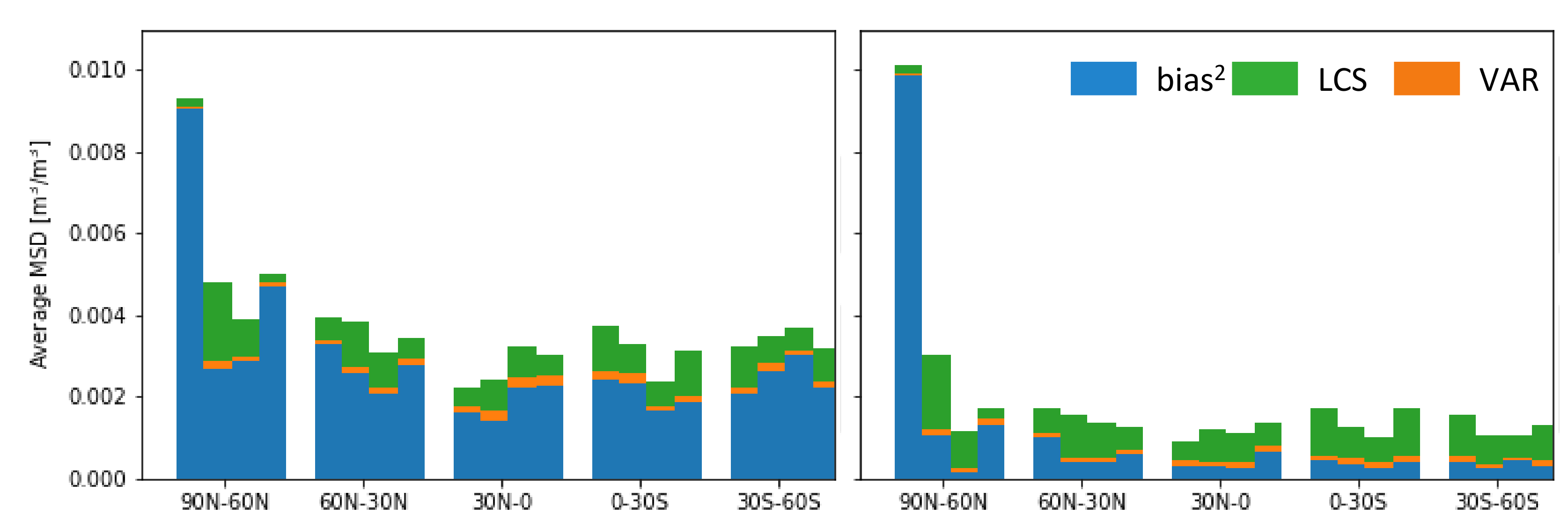
2.4.5. MSD Decomposition

Following [56], we can decompose the mean standard deviation (MSD = RMSD${}^2$) into three informative components. Let $x_{i,t=1\dots n}$ and $y_{i,t=1\dots n}$ denote the two datasets, then

$$\begin{array}{cc}\hfill \mathrm{MSD}& ={(\overline{x_i}-\overline{y_i})}^2+{({\sigma }_{x_i}-{\sigma }_{y_i})}^2+2{\sigma }_{x_i}{\sigma }_{y_i}(1-r)\hfill \end{array}$$

(10)

$$\begin{array}{c}={\mathrm{bias}}^2+\mathrm{VAR}+\mathrm{LCS}\hfill \end{array}$$

(11)

where the bias = ($\overline{x_i}-{\overline{y}}_i)$, $\mathrm{VAR}={({\sigma }_{x_i}-{\sigma }_{y_i})}^2$ and $\mathrm{LCS}=2{\sigma }_{x_i}{\sigma }_{y_i}(1-r)$.

The first term of the decomposition is the squared bias. The second term, VAR, shows the difference in the magnitude of fluctuation between the simulation and measurements. The larger this term, the more the model fails to simulate the magnitude of the fluctuation among the n measurements. The last term of the decomposition is the Lack of Correlation weighted by the Standard deviations (LCS). This term is large when the model fails to simulate the pattern of fluctuation across the n measurements [56].

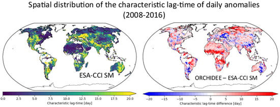
2.4.6. Autocorrelation and Lag Time

For a dataset $x_{i,t=1\dots n}$, the lag-k autocorrelation coefficient can be expressed as:

$$r_k=\frac{{\sum }_{t=1}^{n-k}{((x_{i,t}-\overline{x_i})-(x_{i,t+k}-\overline{x_i}))}^2}{{\sum }_{t=1}^n{(x_{i,t}-\overline{x_i})}^2}.$$

(12)

Following [57], we define the characteristic lag time ($c_t$) as the time at which the autocorrelation coefficient reduces to below $e^{-1}\approx 0.37$. This is also known as the e-folding time. This quantity determines a threshold after which the dataset is no longer considered as significantly autocorrelated. This can thus be seen as a way to quantify the inertia of the studied variable. This metrics is applied to the fast-varying component of the data.

2.4.7. Singular Value Decomposition

Singular Value Decomposition (SVD) offers an adequate tool to analyze the temporal co-variability between two gridded datasets. A detailed description of the method can be found in [58]. The spatio-temporal analysis will consider the total explained covariance of the two fields that is explained by the decomposition into pairs of optimally correlated observation and model patterns, as well as homogeneous correlation maps (depicting the geographic localization of the covarying parts of observation and model respectively) and observation heterogeneous correlation maps (reflecting how well observations are predicted by model patterns). Since the SVD analysis concerns itself with spatial patterns, the SVD algorithm is directly applied to the raw data instead of using the CDF-matched data. This is because the rescaling is applied pixel by pixel and hence would affect the spatial distribution.

3. Results

3.1. Rescaling the ESA-CCI SM Product

Since the ESA-CCI SM product has undergone a rescaling process with the GLDAS-Noah LSM, a direct comparison with the ORCHIDEE model outputs is likely misleading as those models have different soil representation: spatial distribution, textural and hydraulic properties and vertical discretization. In this context, agreement between the ORCHIDEE and ESA-CCI SM products should only be evaluated in terms of relative dynamics unless the observations are first bias corrected or scaled to be consistent with the model climatology. Bias correction is also vital for future data assimilation experiments. Most data assimilation algorithms assume that the uncertainties in the retrievals and the model output are Gaussian distributed, bias correcting the retrievals ensures this condition is satisfied.

In Figure 1 we consider how different scaling algorithms introduced in Section 2.4.1 affect the ESA-CCI SM values. Since the rescaling used in the creation of ESA-CCI product was applied individually at every pixel, we also do the same. Three different scaling are considered. The first rescaling translates both the ESA-CCI and the modelled values to soil water index (SWI) values. Calculated using the minimal and maximal SM values as proxy for the residual/minimum and volumetric field capacity respectively, the values obtained are between 0 and 1. Since the residual value and volumetric field capacity vary between land-surface models, through this rescaling, the ESA-CCI values remain within the GLDAS-Noah climatology. This scaling is more of a type of normalization than a type of bias correction. The second type of rescaling, referred to as linear CDF-matching, matches the mean and standard deviation of the ESA-CCI SM values to that of the modelled values (as described in Section 3.1). The third type of rescaling considered here, is a more complex full CDF-matching which is a refinement of the linear approach, but also matching higher moments of the distributions such as skewness and kurtosis. This latter algorithm for CDF-matching is a non-linear transformation, and as such we can expect small changes in the relative magnitude of the temporal dynamics [35]. Since a full CDF-matching was used in the creation of the ESA-CCI product, it follows that this is the best suited method for rescaling the data to the ORCHIDEE climatology. It is also the method using in several SM assimilation studies e.g., [59,60,61].

The histogram for the ESA-CCI soil moisture values prior to any rescaling is binomial with the second peak (around 0.22 m${}^3$/m${}^3$) much larger than the peaks seen for the modelled soil moisture values (Figure 1). When translated to SWI values, this second peak is lost as the histogram is flattened. After the rescaling using CDF-matching, this peak is split in two to match the three narrower peaks observed in the modelled data. Using the linear CDF-matching, the total global RMSD over the whole 8-year period drops from 0.059 m${}^3$/m${}^3$ to 0.039 m${}^3$/m${}^3$, which equates to a 34% discrepancy reduction. Logically, the SM density distribution overlapping increased from 68.3% to 87.9%, associated with the creation of a third intermediate peak. This similarity between the distributions at this stage is promising. It assures us that the observed and modelled SM values are already relatively consistent and can be compared and used in the future to further optimize model parameters and bring potential improvements. When applying the full CDF-matching, the distributions are nearly identical.

The MSD decomposition shown in Figure 2 illustrates how the full CDF-matching performs at different latitudes focusing on one year (2016). Prior to this rescaling, we can see that bias makes up most of the error. On average it makes up over 72% of the MSD. Errors are particularly high in the northern latitudes for the winter months (January–March). This is because of snow and frozen areas found at these latitudes. In ESA-CCI SM product, points with high levels of uncertainty are flagged and removed. Similarly, using the model output, points where surface temperature is lower than negative one are also removed. Therefore few data points remain to calculate the average MSD in this area during this season as can be seen in

Table A1. Number of points used in the MSD decomposition shown in Figure 2.

	90 N–60 N	60 N–30 N	30 N–0	0–30 S	30 S–30 N
Jan–Mar	34	10,662	9398	6543	1874
Apr–Jun	9212	19,385	9578	6531	1866
Jul–Sep	9597	19,456	9557	6501	1820
Oct–Dec	3310	17,003	9545	6528	1865

. Otherwise, errors are relatively consistent at each of the latitude and over each three-month period prior to rescaling.

In each case, the discrepancy is reduced after the full CDF-matching. Each decomposition still displays a bias component, it on average makes up 37% the bar. This is because the rescaling is done using data from multiple years whereas the figure only displays one single year, and therefore the remnant bias is the bias with respect to the yearly average. Generally, for each latitude-month (one bar), most of the bias is removed, VAR decreases slightly and the LCS portion of the MSD remain the same size. This shows that overall correlation amplitudes are relatively insensitive to this choice of rescaling.

Spatial correlations were also considered between the model and ESA-CCI SM values both prior to and after rescaling. Before rescaling, mean spatial correlations globally range according to a seasonal cycle between 0.66 and 0.86. After rescaling, these values follow the same pattern but drop between 0.50 and 0.79 for the SWI algorithm and increase to between 0.82–0.95 for both versions of CDF-matching.

For the remainder of this paper, unless stated otherwise, the rescaled ESA-CCI SM values obtained through the full CDF-matching are the ones considered.

3.2. An Analysis of Model Depth Selection

We investigate in this section the effect of integrating the model soil moisture over different depths. The reference depth is 2.2 cm, corresponding to the 4 top layers (see Section 2.3). We first consider the RMSD with the reference depth that makes the most theoretical sense (Figure 3a). The lowest errors are observed in the Sahara and other desert areas. RMSD is relatively low in these dry areas, with errors averaging 0.017, since these places will have low SM values. The largest values of RMSD of about 0.15 tend to be found in the northern latitudes and along the Himalayan mountain range. These are snowy regions and, as discussed previously, these may be areas where most of the model and ESA-CCI SM values are flagged. There are also a few areas with higher RMSD values near the masked areas of dense vegetation (i.e., Brazil and central Africa). The rest of the map shows a relatively constant error close to 0.04 m${}^3$/m${}^3$.

When considering the standard deviation globally in Figure 3b, we can see that there is little to no variation in RMSD between layers. Indeed, for 50% of the map, the standard deviation between layers is less than 0.001 m${}^3$/m${}^3$. This proportion increases to over 90% of the map for standard deviations less than 0.003 m${}^3$/m${}^3$. The highest scores of around 0.01 (less than 0.12% of the points globally) can be found in some of the dry areas. These RMSD values remain low considering the values of soil moisture are of magnitude $\mathcal{O}$(0.1) m${}^3$/m${}^3$. The consistency in RMSD values over these first few layers of the model may be partly due to the use of daily averages. It is possible that we may see variations at different depths if we could get instantaneous values for the different rainfall events. However, since the ESA-CCI SM product currently only provides daily values, we cannot reduce our time step.

With the first few layers virtually the same, even though the errors are slightly lower calculated over the top 5 layers, we choose to keep using the top 4 layers in our analysis since this depth makes the most theoretical sense [32,62]. Therefore, for the remainder of this study, a depth of 2 cm (top 4 layers in the model) is used.

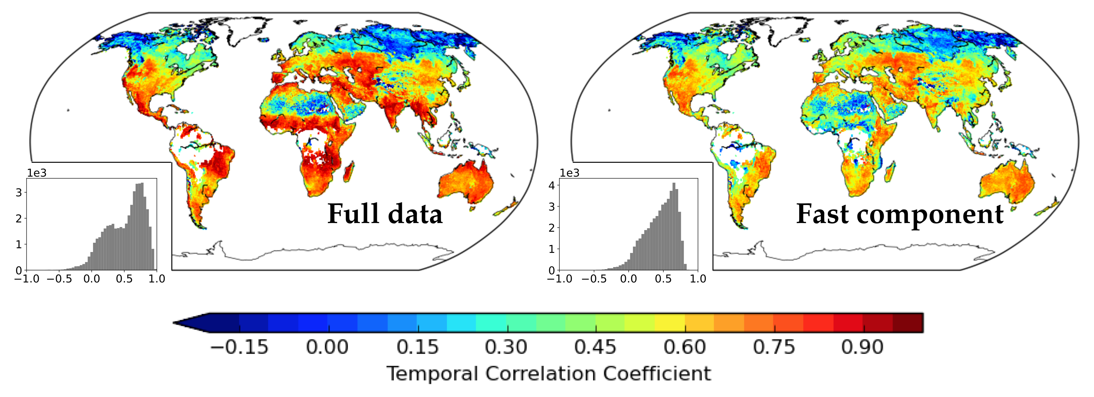
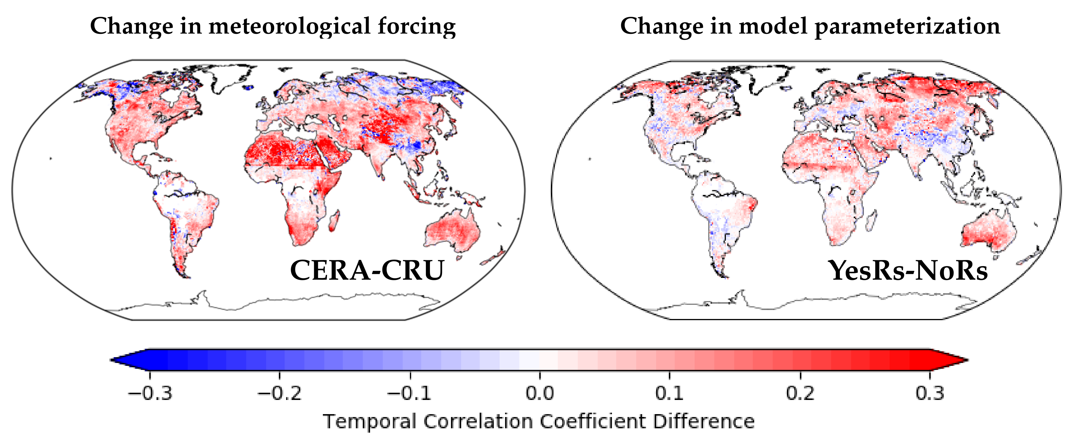
3.3. Mean Temporal Correlations between Model and ESA-CCI SM Product

Due to the rescaling process undergone to create ESA-CCI SM product, as well as the rescaling procedure implemented, considering the RMSD between the observations and modelled time series is not the most informative metric. Temporal correlation, on the other hand, evaluates the agreement between the ORCHIDEE and ESA-CCI SM product in terms of relative dynamics and therefore is less sensitive to the choice of rescaling. Overall, we can see strong correlations between the model output and the ESA-CCI SM values (Figure 4). Highest correlations are found in the tropics and southern latitudes when the average correlation score is 0.7. Temporal correlations are highest over areas where remote sensing methods are known to be efficient. Poorer results are found over desert, mountainous and frozen areas. In desertic areas, this may be explained by forcing errors, i.e., the precipitation used to drive the model. Rain is spatially heterogeneous over deserts with few events, these can be hard to observed, and hence can be a large source of uncertainty over such regions. Furthermore, the satellite representative depth over deserts tends to be larger in dry conditions and the larger surface ground heating during the day may also increase the errors on the retrievals [43]. The poor results in mountainous and frozen areas can be partly explained by the difficulty to model the radiative transfer in those conditions (i.e., separate roughness and soil moisture effects), and therefore to inverse SM from remote-sensed data. This is particularly noticeable in the high latitudes where the average correlation reduces to 0.15 compared to the global mean of 0.49. In lines with previous studies, best scores are obtained in areas with strong annual cycles and higher density data [32].

For the purposes of data assimilation, we are interested in the sub-monthly variations. From Figure 4 we see that the sub-monthly variations are less correlated than the full data. The histograms show that for the full data, there is a peak large at 0.76. For the anomalies, the peak is lower found at 0.63. The full data reaches close to values of one whereas the fast component does not exceed 0.9. The differences observed between the full data and the fast component highlight the fact that factors such as the spatio-temporal variability of precipitation strongly affect the temporal correlations. Though not shown here, the correlations found here are nearly identical to correlations calculated at the other depths between layers 2 and 7. This is also the case when considering the raw and different rescalings of the ESA-CCI SM data. The full CDF matching used to rescale the observations can have a slight effect on the temporal dynamics. However, since the strong correlations are also observed when the raw ESA-CCI values are used, we can be confident that the strong correlations are due to the agreement between the model and satellite data instead of the rescaling procedure itself.

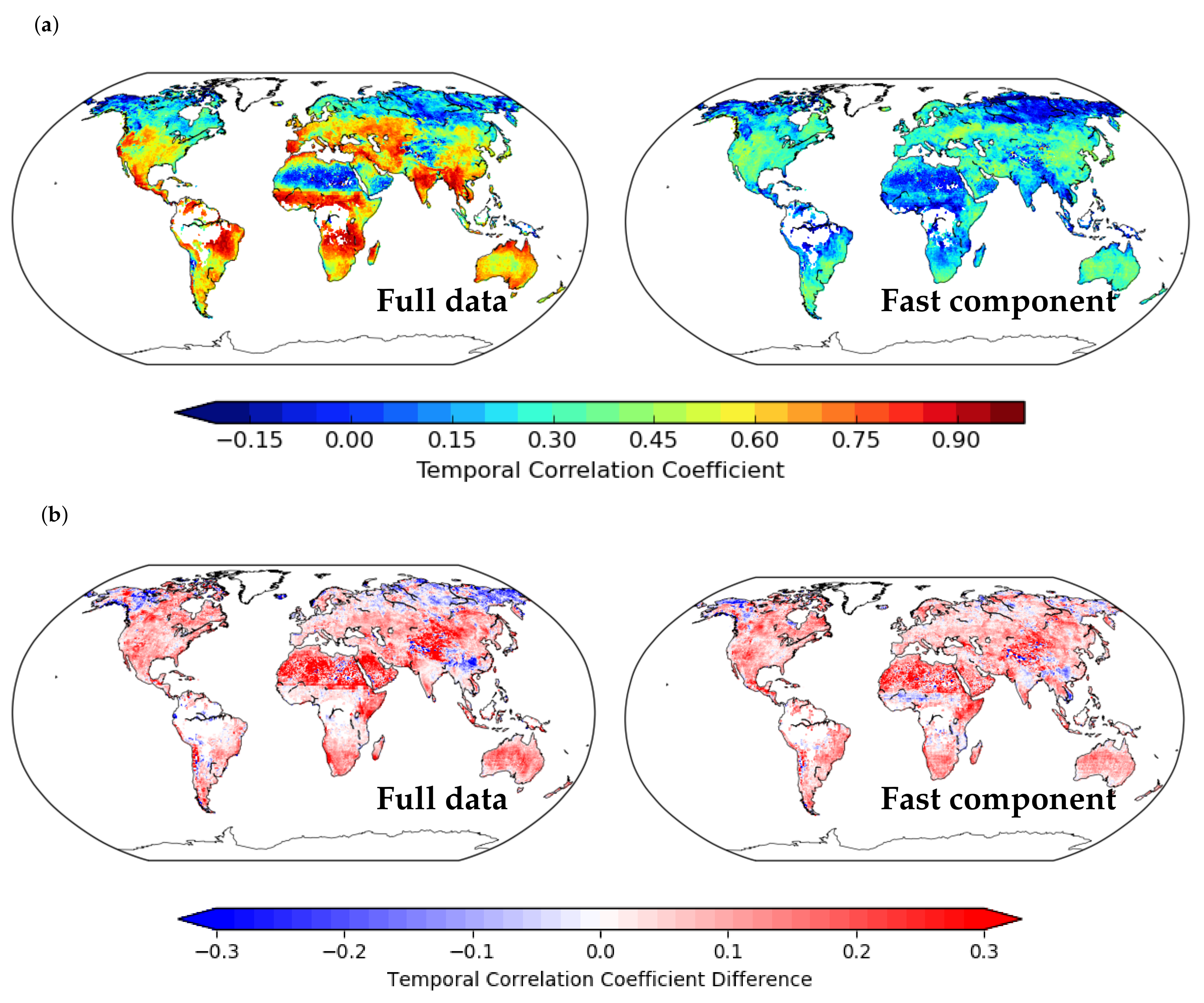
3.4. The Effect of Meteorological and Land Cover Forcing Data

The choice of forcing data heavily influences the simulation of SM in LSMs. In this section, we first compare our default ORCHIDEE run ORC_REF to one with a different meteorological forcing, CRUNCEP, introduced in Section 2.3. From Figure 5 we can see that the ORC_REF run outperforms the ORC_CRU for the full data and the fast component. This is particularly notable in arid or desert regions (i.e., Sahara, Asia, and Australia). ORC_REF shows stronger correlations than ORC_CRU for the fast component. This shows that the ORCHIDEE run using the CERASAT meteorological forcing not only captures the same seasonal patterns as the satellite data but also more of the sub-monthly behavior of SM.

CERASAT is a new dataset of the ECMWF based on recent advances in data assimilation and uses satellite data in its creation. Another reason for the CERASAT forcing data outperforming CRUNCEP may be due to the difference in temporal resolution between both products. CERSAT is 3-hourly whereas CRUNCEP is 6-hourly. This difference in frequency may affect how the precipitation is partitioned for each different time step and hence the response of SM in the model. The noticeable differences between the correlations for each run show that the choice of meteorological forcing is critical for the accurate simulation of SM. Many studies have in fact used SM to correct precipitation input [63,64,65,66,67]. Conversely, to correct the SM parameters in ORCHIDEE, it is important to find a metric that is less sensitive to the meteorological forcing.

Forcing data is not limited to the meteorological data used to drive the model. It encompasses all external data used for a given model run. Another dataset used as forcing data in ORCHIDEE is the choice of land-cover map, which determines the distribution of the global vegetation. In this study, we only tested two slightly different land-cover maps, and the correlations between the ESA-CCI SM product and ORCHIDEE SM output remained very similar. This suggest that, in this case, the choice of land cover is not the primary source of variability.

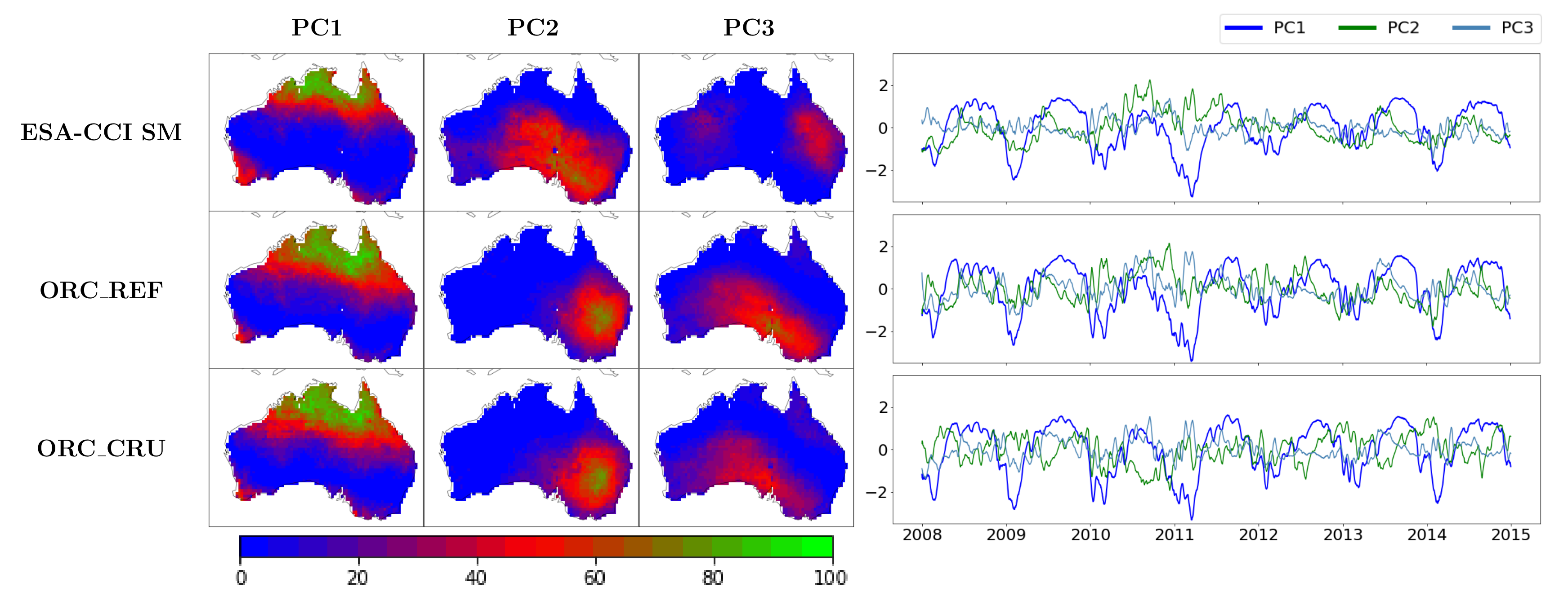
3.5. Measuring the Covariance of Rainfall and Soil Moisture

The chosen meteorological forcing data prescribes (among others) the precipitation in the model. Since precipitation, both the amount and intensity, has been shown to be a major driver to surface soil moisture dynamics [68], this dependency can be assessed through their covariance. Following [69], we use the SVD method described in Section 2.4.7 to identify and study coupled rainfall-SM covarying spatio-temporal patterns. To ensure that the comparison does not favor the model output and that therefore any differences found originate from the SM only [69], independent rainfall data is needed. For this experiment, it was provided by MSWEP data and the period 2008–2014 was considered because it overlaps all datasets.

We focus our analysis over Australia and the Iberian Peninsula. Australia was selected since the ESA-CCI SM product has shown a good performance over this country in terms of correlation with reanalysis and in situ datasets [35,36]. Also, passive, active, and combined products have all been used over this region [70] resulting in the fractions of days with valid observations to be very high [35]. Therefore, we can expect a reliable quality of the product over this region. The Iberian Peninsula was selected to provide direct comparison with [69] who used satellite SM values from the ESA’s Soil Moisture and Ocean Salinity product (SMOS-BEC).

Considered in

Table 3. Characteristics of the first three pairs of covarying patterns of precipitation (P) and SM over Australia and the Iberian Peninsula for 2008–2014. Explained (co-)variance are shown in percentage. Found in bold are the total explained (co-)variances and mean correlation scores.

Data	Covarying Pattern	Explained Covariance	Explained Variance of SM Patterns		Correlations between Covarying Patterns of SM and P
			by Precip. (Heterogeneous)	by SM Itself (Homogeneous)	Spatial	Temporal (Expansion Coeff.)
Australia
ESA-CC1	PC1	85.2	12.73	21.71	0.92	0.76
	PC2	5.15	4.05	23.6	0.84	0.42
	PC3	4.55	2.34	9.87	0.92	0.5
		94.9	19.12	55.18	0.89	0.56
ORC_REF	PC1	81.97	20.61	29.46	0.90	0.83
	PC2	6.77	4.01	13.82	0.95	0.56
	PC3	5.03	5.50	17.97	0.92	0.57
		93.77	30.12	61.25	0.92	0.65
ORC_CRU	PC1	86.69	19.91	29.76	0.87	0.80
	PC2	5.08	3.01	15.37	0.92	0.46
	PC3	3.50	3.50	14.27	0.86	0.52
		95.27	26.42	59.40	0.88	0.59
The Iberian Peninsula
ESA-CC1	PC1	96.78	15.89	75.81	0.56	0.46
	PC2	1.65	1.39	8.89	0.89	0.4
	PC3	1.04	0.82	5.25	0.87	0.41
		99.47	18.1	89.95	0.77	0.42
ORC_REF	PC1	95.12	23.68	81.96	0.52	0.54
	PC2	2.52	3.11	12.4	0.95	0.52
	PC3	1.79	2.29	8.36	0.96	0.54
		99.43	29.08	102.72	0.81	0.53
ORC_CRU	PC1	95.71	18.99	80.24	0.68	0.49
	PC2	2.12	1.71	11.92	0.89	0.42
	PC3	01.58	1.51	10.15	0.94	0.44
		99.41	22.21	102.31	0.84	0.45

are the first three covarying patterns representing approximately 95% and 99% of the covariance of SM and P for Australia and the Iberian Peninsula, respectively. The explained covariance is of the same proportion whether the ESA-CCI product is considered, or whether the different model runs are considered. For the Iberian Peninsula, most of the covariance is explained by PC1. When the SM time-expansion coefficients are plotted, (see Figure 6) we can identify a large annual cycle in PC1. PC1 therefore represents the seasonal co-variability of rainfall and SM. The usually shallow trough observed in 2012 corresponds to the severe drought that Spain experienced with precipitation less than 30% than its normal amount between December and February. PC2 and PC3 represent the higher frequency (synoptic) variability of SM linked to rainfall events.

For Australia on the other hand, PC1 still explains most of the covariance; however, PC2 and PC3 also explain a small part. From Figure 7, PC1 appears to be explaining the monsoon events occurring in north-east Australia. The pronounced trough seen in late 2010/early 2011 correspond to the Australia floods of 2010–2011. These floods were due to unusually heavy and prolonged rain caused by the seasonal wet monsoon coinciding with an unusually strong La Niña events [71]. The spatial representation of the PC1 for the ESA-CCI SM suggest that the monsoon comes down too low in both versions of the model runs. PC2 and PC3 described the rainfall patterns found in the south and southeast.

By considering the spatial patterns in Figure 6 and Figure 7, we can see that PC2 and PC3 for the ESA-CCI SM and the models are reversed for both Australia and the Iberian Peninsula. The PCs are ordered by the amount of explained covariance. For Australia, the satellite product suggests that the rainfall in the south explains more of the covariance than the rainfall in the south-east, whereas the models suggest the opposite. For the Iberian Peninsula, the ESA-CCI SM product highlights the Mediterranean coastal rainfall explaining more than the rainfall over the Pyrenees. However, when we consider the values of explained covariance in Table 3 we can see that the difference between the two PCs is negligible.

The homogeneous explained variance fraction in Table 3 refers to the SM variance explained by the soil moisture itself. The soil moisture PC1 for the Iberian Peninsula and Australia explains a slightly higher proportion of the total SM variance when using the model runs that the ESA-CCI product; 81% compared to 76% for the Iberian Peninsula and 30% compared to 23% for Australia. This slight discrepancy between the satellite observations and models is consistent with [69]’s findings and similarly suggests that there are structures that are not rainfall-driven captured by the satellite product that are missing in the model.

The heterogeneous explained variance fraction in Table 3 refers to the SM variance explained by the rainfall. For both the Iberian Peninsula and Australia, the PCs show a slightly weaker link between rainfall and SM for the satellite data than for the model. The sub-seasonal variability of precipitation extracted by the SVD analysis (shown by PC2 and PC3) seems to explain a negligible part of the SM variability. This is because the seasonal variations of the precipitation are better represented than the higher frequencies due to the precipitation’s high spatio-temporal variability.

The best thing that can explain the variance in the SM patterns is SM itself. Therefore, the values for homogeneous explained are the highest possible. The fact that, for Australia, the precipitation can explain the variance of the SM pattern by the same magnitude as SM itself, clearly shows that precipitation is the main driver of SM in this region. For the Iberian Peninsula, the precipitation explains nearly the same amount of the SM pattern variance as it does for Australia, but this is only a third of the homogeneous values.

The spatial correlation values are stronger for Australia than for the Iberian Peninsula. One of the reason we observe higher spatial correlations in our analysis may be due to topological and land-use differences between Australia and the Iberian peninsula. Australia has more homogeneous and natural landscape, whereas the Iberian Peninsula has more irrigation, lakes, mountainous areas in a smaller area.

As observed in [69], we find that the slow-varying PC1 for the Iberian Peninsula is less spatially correlated than the fast-varying PC2 & 3. Since the PC1s represent the seasonality for the Iberian Peninsula, the variability represented is determined not only by rainfall, but also by other processes such as evaporation and drainage. These processes are less important for the fast-varying PCs. In contrast, for Australia, we find that spatial correlations of each of the PCs show the same magnitude in each of the datasets. This may be due to the fact each of the PC1s for Australia is representative of different rainfall types. Overall these spatial correlations are stronger than those observed in [69]. In [69], the SVD analysis was conducted using SMOS, a pure remote sensing estimate, whereas we are using a merged product where a model has been used. It is possible that the usage of the GLDAS-Noah model in the merging process has smoothed out a large part of the spatial variability associated with landscape features or measurement noise.

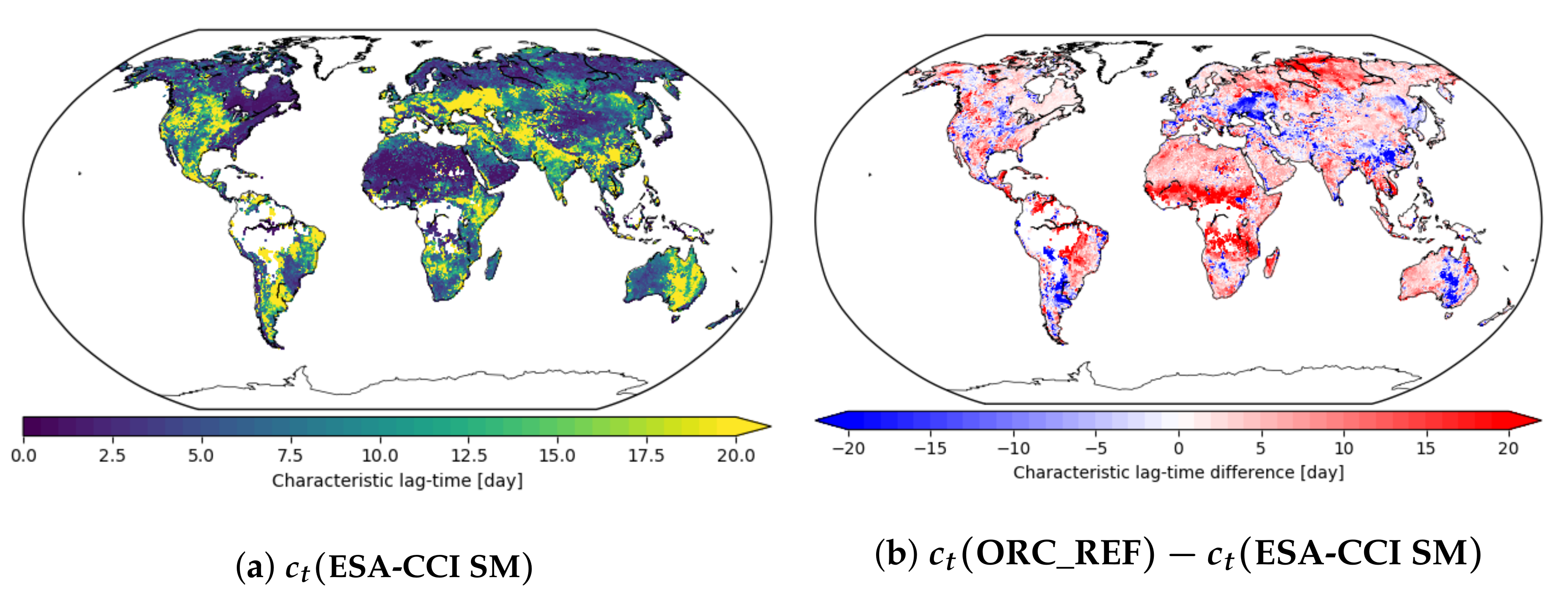
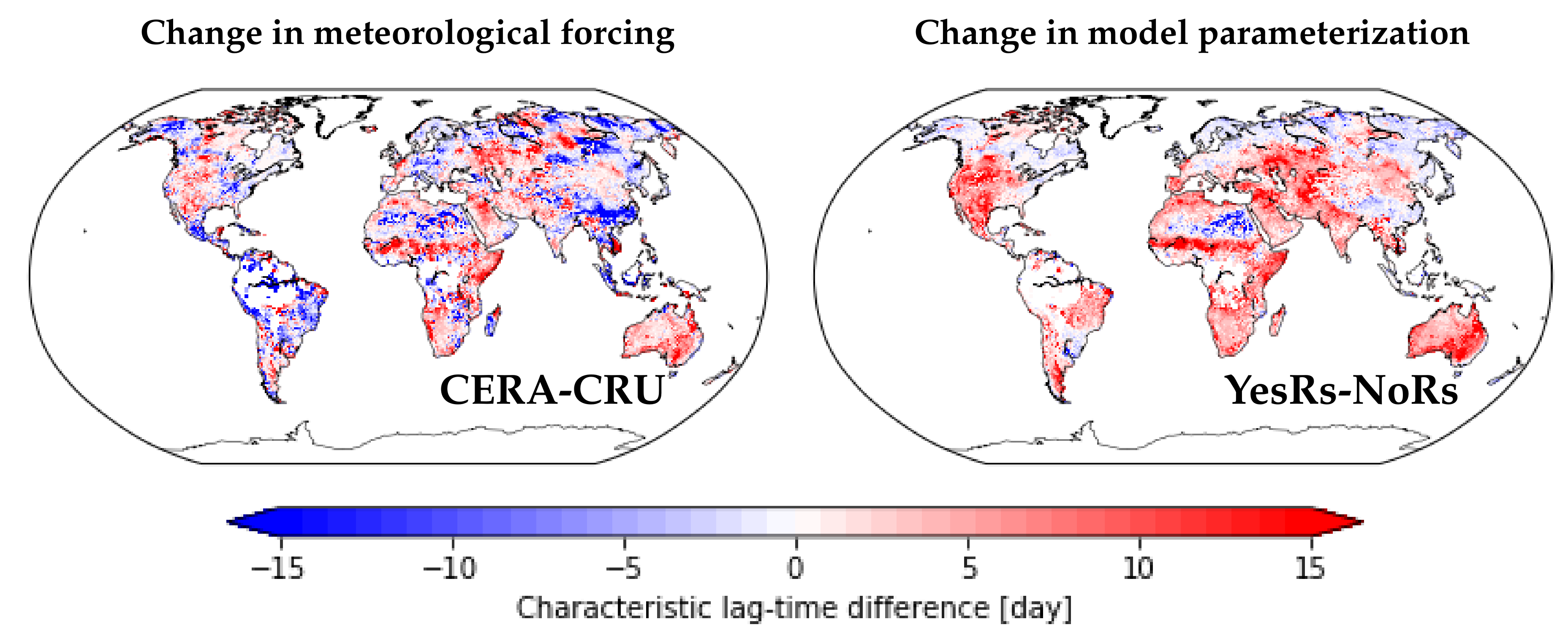
3.6. Temporal Autocorrelation

The strong correlations found between the ESA-CCI SM product and the ORCHIDEE output are very promising. In this section, we further investigate the temporal autocorrelation, a similar metric that should also be insensitive to the choice of rescaling. It represents the correlation of a variable with its own future and past values [72]. Intuitively, since SM temporal autocorrelation should be more controlled by processes such as evaporation and drainage, it should be less sensitive to the choice of meteorological forcing and more sensitive to the choice of parameterization used in the model.

Temporal autocorrelation, and thus characteristic lag time, is a relatively simple metric but with potentially complex interpretations which can integrate notions of dry-down. Temporal autocorrelation, in cases when the interval between precipitation events is large enough, can sometimes be interpreted as a useful indicator of SM inertia (i.e., persistence and depletion time), less influenced than correlation metrics by the climate forcing; it should allow to assess more precisely the model’s structure. In past studies, people rarely used such analysis, probably because it often leads to large disparities between modelled and observed products (see for example [12]). Such disagreements could be explained by the gap between the observed representative depth and the simulation depth. It is indeed well-known that depth has a major influence on the inertia of SM [69]. However, we have shown in Section 3.2 that signal representative depth in ORCHIDEE for daily SM value is relatively consistent.

The characteristic lag time $c_t$ defined in Section 2.4.6, is a measure of temporal decorrelation rate. More specifically, it measures soil moisture memory which can be partly related to the time taken by the soil to ‘forget’ an anomaly [73]. $c_t$ of the ESA-CCI SM product varies greatly depending on different regions (Figure 8a). Areas with the longest $c_t$, between 15 and 30 days, tend to be regions with a temperate climate. Shorter $c_t$ times occur in areas with a drier climate, for example 1.4 days over the Sahara, where there is less rainfall. Figure 8b allows us to compare $c_t$ for the model run and the ESA-CCI product. Overall there is higher SM stability in the model than in the satellite product (red areas in Figure 8b), though parts of Australia, South America and Asia are modelled as more reactive (blue areas in Figure 8b). The model predicts much higher characteristic lag-time values around the tropics than the ESA-CCI SM, mainly around the masked dense vegetation; these values can differ up to 15–20 days. On average; however, the differences between the model and the product tend to be of the order 4–5 days.

3.7. Potential Impact of Parameterization on SM Dynamics

In this section, we consider the effect of removing the $r_{\mathrm{soil}}$ parameterization from the model (see Section 2.3), as was chosen for a configuration of ORCHIDEE in the IPSL-ESM for the CMIP6 exercise. This is not exhaustive but will help to illustrate the impact that changing a parameterization can have on SM dynamics. The soil resistance term in the model will control how long the soil moisture is kept in the first few centimeters of the soil. Water is removed from these centimeters either by evapotranspiration into the atmosphere, by vertical infiltration into the deeper layers of the soil or by surface-runoff to rivers. When comparing ORC_REF to ORC_NoRs (an ORCHIDEE run without soil resistance, Figure 9), since both versions of the model runs use the same PFT and soil maps, and same topography, the evapotranspiration will be the flux quantity that differs the most between the different model runs.

Evapotranspiration comprises soil evaporation and plant transpiration. In arid regions, since soil evaporation is dominant, it will have a larger control on SM than in vegetated areas where transpiration will play a key role. When soil resistance is not included in the model (i.e., ORC_NoRs), evaporation rates are higher and therefore the SM in the model will dry out faster. This is why for ORC_NoRs, arid regions, where evaporation dominates the total evapotranspiration, show the greatest difference in characteristic lag time between the run and the ESA-CCI values. The differences in the characteristic lag-time values for ORC_NoRs and ORC_REF are of the same magnitude as the differences between ORC_NoRs and the ESA-CCI values. This shows that adding or removing a parameterization can largely affect SM output and thus structural model changes need to be considered before parameter estimation experiments.

When considering the difference between the autocorrelation lag time of the model and the ESA-CCI product for the different meteorological forcings, similar regional patterns are identified. However, when taking the difference between both model runs(i.e., ORC_REF and ORC_CRU), the intensity is seen to differ (Figure 9). The forcing induced difference is also comparable in magnitude to the difference between two model runs with different parameterizations (with change in model parameterization being slightly stronger; the average global absolute difference is of 5 days compared to 4 days). Without the soil resistance parameterization, the $c_t$ values are much lower nearly globally. Changing the meteorological forcing or the model parameterization in this example affects different regions. For example, the characteristic lag time of south China is more sensitive to the meteorological forcing than the soil resistance term. In contrast, the Australia $c_t$ value is more affected by the parametrization change than the change in meteorological forcing. This is an example where the autocorrelation metric is sensitive to the specifically selected parameterization. Since the characteristic lag time was shown to differ between the different configurations of the model and the satellite observations, it is potentially a useful metric to identify and correct systematic errors and parameters in ORCHIDEE.

In contrast, if instead we consider the correlation metric, as shown in Figure 10, we observed that changing the meteorological forcing has a greater effect on the correlation scores than changing the model parameterization. The global mean absolute difference in correlation score is 0.11 for the meteorological forcing compared to 0.07 the parameterization change. This increases to 0.25 over the Sahara compared to 0.08. In this example, the correlation metric is more sensitive to the meteorological forcing used and it may be harder to use this metric to pick out the internal deficiencies of the model but would be more appropriate if one wanted to diagnose or correct input precipitation data.

The choice to include or exclude soil resistance will also have a direct effect on the carbon cycle. As such, to conclude this section, we consider how different vegetation (based on maximum leaf area index values LAI${}_{\mathrm{MAX}}$) and soil classes perform with respect to the ESA-CCI product and the different metrics discussed (see

Table A2. Properties for different classes of maximum LAI and soil textures. All values correspond the mean calculated over all the points in each class. Each metric is calculated between the model (both ORC_REF and ORC_NoRs runs) and the rescaled ESA-CCI SM product (in each case, CDF-matched to the corresponding ORCHIDEE run). The distribution of the different classes is displayed in Figure A1.

Index	Range Covered	% of Points		r		RMSD		${\mathit{c}}_{\mathit{t}}$ (Mod)		$\mathbf{\Delta }{\mathit{c}}_{\mathit{t}}$ (Mod-Obs)
		REF	NoRs	REF	NoRs	REF	NoRs	REF	NoRs	REF	NoRs
1	${\mathrm{LAI}}_{\mathrm{MAX}}<0.5$	29.0	25.0	0.47	0.37	0.029	0.033	9.605	6.744	4.859	1.969
2	$0.5\le {\mathrm{LAI}}_{\mathrm{MAX}}<2$	28.0	27.0	0.46	0.38	0.038	0.049	12.14	8.017	2.768	−0.760
3	$2\le {\mathrm{LAI}}_{\mathrm{MAX}}<3$	23.0	25.0	0.51	0.47	0.037	0.046	11.841	9.711	1.744	−0.244
4	$3\le {\mathrm{LAI}}_{\mathrm{MAX}}$	18.0	21.0	0.67	0.68	0.038	0.043	14.943	12.631	1.796	−0.166
1	Coarse	25.0	25.0	0.50	0.46	0.028	0.029	8.217	5.719	2.756	0.254
2	Medium	62.0	62.0	0.49	0.44	0.037	0.049	12.392	9.734	2.768	0.111
3	Fine	11.0	11.0	0.68	0.65	0.038	0.042	17.380	13.497	4.207	0.350

in Appendix A). The strongest correlations are found at points where LAI${}_{\mathrm{MAX}}\ge 3$ or where points have a fine soil texture. Areas with finer soil textures tend to have the most fertile soils and hence vegetation with the largest LAI. These regions, found in the temperate and tropical zones, have precipitation regimes with frequent rainfall events. The RMSD is relatively consistent over the different vegetation and soil texture classes considered, though slightly lower in areas with sparse vegetation (LAI${}_{\mathrm{MAX}}<0.5$) and coarse soils. These areas include desert areas where soil moisture values will be very low. The average RMSD is slightly higher for the run without the soil resistance parameterization. The characteristic lag time increases with increasing LAI${}_{\mathrm{MAX}}$, and these values are higher when using soil resistance in the model compared to running the model without soil resistance. When LAI${}_{\mathrm{MAX}}<0.5$, these pixels will be close to having bare soil. With increasing LAI${}_{\mathrm{MAX}}$ values, the vegetation will become more complex (for example with larger roots) as will the processes involved in control the soil moisture. Characteristic lag time is also highest for fine soil textures which have a higher water-holding capacity and lower hydraulic conductivity. The average characteristic lag-times for the model differs the most in areas with sparse vegetation or areas with fine soils, and more for the ORC_REF (with soil resistance) than for the ORC_NoRs run (no soil resistance).

4. Discussion

Throughout this paper, we have been assessing the potential of the ESA-CCI SM product to be used to evaluate and further improve the ORCHIDEE LSM. A first step in doing so, was to rescale the observations to the climatology of the ORCHIDEE model. This is necessary due to the steps undergone to create the ESA-CCI SM product: i.e., active and passive satellite retrievals were combined using the climatology of the GLDAS-Noah model reanalysis. Since this model has its own soil moisture climatology with different dynamical ranges [74], it is important to rescale data to the ORCHIDEE’s climatology. In addition to the rescaling undertaken in creating the ESA-CCI product, there are also biases due the satellite signal processing. SM is estimated through inversion procedures based on radiative transfer modelling. This procedure uses additional assumptions and data such as vegetation distribution maps. For data assimilation studies, proper treatment of systematic errors is critical for the success of the experiment [75]. Since Gaussian error statistics is one of the key assumptions of most data assimilation systems, bias correction is a vital first step. However, it is worth noting that any form of bias correction will not only correct systematic biases and the biases due to the climatology mismatch but will also remove biases linked to the ORCHIDEE model itself. In an ideal case, using DA techniques, we would correct this latter source of bias. Since it is impossible to distinguish between sources of biases, we accept that, through the rescaling, we lose some of the information contained in the observations that could have potentially, corrected parts of the model. This choice is common practice when using satellite products even though it has been shown that the current bias-correction methods may remove up to 50% of information from the original satellite observations [76,77].

Since the microwave instruments used to generate the ESA-CCI product, are only able to monitor a thin surface layer, it was important to assess which depth has to be considered in the model. Fortunately, the first two meters of the soil column in ORCHIDEE is discretized by an 11-layered hydrology scheme, allowing us to select the corresponding depth. When unable to directly match the sensing depth, or when one wants to constrain model SM further down the soil column, a potential approach to the issue of representativity is to use an exponential filter [44]. This method translates the SM observed in the top few centimeters by the satellites to the SM representative of deeper layers following certain exponential assumptions. Such exponential filter has been used in several previous DA studies e.g., [55,78,79]. Since we can directly match the sensing depth in this study, we simply use the first four layers of the ORCHIDEE soil column discretization to perform the intercomparisons.

Comparison scores were found to be very similar at different depths of ORCHIDEE soil column. Since this trend was observed globally, this is the case when both the passive satellites dominate the product (i.e., over deserts) and when the active retrievals dominate the combined product (i.e., over high latitudes). The merging process may have contributed to the smoothing of the depth profile, as might the fact that the product only provides daily values. The first 4 layers of the model’s soil column have been evaluated in this study. Although little difference was observed between the different integrated depths, if the data assimilation experiment is conducted at this depth, it will be important to consider its effect of the improvements over the rest of the 11 layers. The soil hydro-thermal parameters are currently homogeneous over the soil column but improving the surface soil moisture may highlight the need for different parameters further down the soil column or lead to conclusions that parts of the model such as the bare soil evaporation or root dynamics need to be modified.

An SVD analysis showed that most of the SM variability could be explained by the precipitation patterns. Since the simulation of SM in the model is driven by precipitation and hence the meteorological forcing data, it is impossible to find metrics unaffected by the forcing errors. Two main metrics were considered: correlation and autocorrelation. Both allow to focus on relative temporal dynamics for the chosen rescaling and they were also found to be consistent over the first few layers of the ORCHIDEE discretization scheme.

The strong correlations between the daily model outputs and the ESA-CCI values were identified. The mean correlation globally for the full data had a value of 0.49, this average increased to 0.7 when considering the tropics and southern latitudes. For the fast component, the mean global correlation was 0.45, and 0.51 over the tropics and south latitudes. Such strong correlations give confidence in both the model and satellite product. However, the correlation metric was shown to be sensitive to the meteorological forcing used, with variations of 10% globally, and therefore not necessarily informative about the model structure and parameter errors. Indeed, we saw when considering the soil resistance parameterization, changing the meteorological forcing had a greater effect on the correlation scores than this structural change. For example, over the Sahara, changing the meteorological forcing saw an average change of 21% in correlation scores compared to a change of 5% found when changing the soil resistance parameterization.

Temporal autocorrelation, which characterizes quickness and extension of SM variations, highlighted different behaviors in the model vs ESA-CCI product. In some areas, the ESA-CCI values are found to be more autocorrelated than the model, and in the others, the opposite is seen. This metric is sensitive to the parameterization of the model that control variables linked to the simulation of SM, such as evaporation, infiltration and drainage. Given the large uncertainties that are still associated with these processes [10,74] using SM temporal autocorrelation to optimize the main parameters involved in these parameterizations, through DA techniques, is promising.

Temporal autocorrelation can be used to measure soil moisture memory and can be related in some cases to notions of dry-out. The characteristic lag-time metric used in this study is one of a number to the measure of these processes. Although it is informative, it has a few limitations. Firstly, since this metric is based on anomalies, to calculate these anomalies, the mean state is removed from the full data. The mean state was averaged only over 8 years of data which is not long enough to properly extract the climatology for regions with high year to year variation in seasonal precipitation. Hence the calculation of the mean state introduces sampling error into the data [73]. Secondly, autocorrelation-based-metrics ignore the sign of the anomaly which can provide physically meaningful information. Other metrics such as mean persistence time can overcome some of these limitations and hence could be interesting metrics to consider in the future [73,80].

We have shown that the choice of parameterization used in the model is vital in the simulation of SM. In our example, removing soil resistance in the model was seen to decrease soil inertia and therefore create greater discrepancies with the ESA-CCI SM values. Of course, other key variables related to water fluxes should be considered for DA such as soil porosity and the other textural properties and hydraulic parameters (saturated hydraulic conductivity and variation with depth according to soil compaction and vegetation roots) as well as plant water uptake parameters such as root profile. The water and energy balance formulations in ORCHIDEE are representative of the equations found in other LSMs (e.g., JULES [81,82], JSBACH [83]) used in wider Earth system models. Therefore, improvements and structural changes highlighted in a future DA study could potentially also be applicable to these other models.

Overall the ESA-CCI product has great potential to identify missing processes and structural issues in the ORCHIDEE model, and potentially to correct the internal model parameters. However, the effectiveness of any data assimilation frameworks relies on the quality of satellite soil moisture observations and assimilation technique used. We will need to quantify the errors in the satellite retrievals to ensure the success of the assimilation, as well as account for forcing errors in the DA scheme.

Improving soil moisture will influence other modelled products such as evapotranspiration and infiltration. It will be important to consider the impact improving soil moisture has on such variables. Incorporating other products in the assimilation process can help ensure the quality of these outputs do not degrade when correcting soil moisture values. In addition, due to SM’s role in driving the terrestrial carbon balance (through photosynthesis, ecosystem dynamics, and soil respiration), SM data has been highlighted as one of the remotely sensed Earth observation products relevant for terrestrial carbon cycle data assimilation [29]. As such, SM data can also be used as one of multiple data streams to improve the carbon cycle. Two approaches exist when assimilating multiple data streams. The first is simultaneously, as shown in [84] where remotely sensed soil moisture data along with in situ atmospheric CO${}_2$ are used to constrain global terrestrial carbon cycle. The second approach is stepwise, by taking each data stream one at a time. This approach is used in [85], where three different data streams are assimilated to constrain the ORCHIDEE LSM’s carbon cycle. A follow up study will consider the addition of SM into the carbon cycle DA system.

Throughout this study, we have focused on off-line runs which use meteorological data to drive the model. Another avenue for further work would be to consider coupled surface-atmosphere runs, which would allow to analyze the role of soil moisture on the atmospheric boundary layer properties and on the generation of precipitation, especially in semi-arid areas where these links are debated [5,9].

5. Conclusions

Even though there have been many studies evaluating the usefulness of the ESA-CCI SM dataset, this study is unique in considering the product on a global scale using a cutting-edge terrestrial CMIP6 model. This global comparison has shown that both the model and the product are at a stage where useful information can be derived and assimilated. The strong temporal correlations seen between the ESA-CCI product and the model show that the dynamics in the model are developed enough to capture the main trends identified by the combined satellite product. This is especially the case when the CERASAT meteorological forcing data was used.

Temporal autocorrelation was identified as a useful metric to investigate the discrepancies in the inertia of SM. Since it measures the response time of the model and in some cases is more intrinsically linked to the internal dynamics of the model, it gives us an opportunity to evaluate the structure of the model more precisely. The focus of upcoming DA studies could be to correct the internal parameters of the model by minimizing characteristic lag-time discrepancies, or similar metrics of soil moisture memory.

References

1. Nemani, R.R.; Keeling, C.D.; Hashimoto, H.; Jolly, W.M.; Piper, S.C.; Tucker, C.J.; Myneni, R.B.; Running, S.W. Climate-driven increases in global terrestrial net primary production from 1982 to 1999. Science 2003, 300, 1560–1563. [Google Scholar] [CrossRef] [PubMed]
2. Booth, B.B.; Jones, C.D.; Collins, M.; Totterdell, I.J.; Cox, P.M.; Sitch, S.; Huntingford, C.; Betts, R.A.; Harris, G.R.; Lloyd, J. High sensitivity of future global warming to land carbon cycle processes. Environ. Res. Lett. 2012, 7, 024002. [Google Scholar] [CrossRef] [Green Version]
3. Le Quéré, C.; Moriarty, R.; Andrew, R.M.; Peters, G.P.; Ciais, P.; Friedlingstein, P.; Jones, S.D.; Sitch, S.; Tans, P.; Arneth, A.; et al. Global carbon budget 2014. Earth Syst. Sci. Data 2015, 7, 47–85. [Google Scholar] [CrossRef] [Green Version]
4. Anav, A.; Friedlingstein, P.; Beer, C.; Ciais, P.; Harper, A.; Jones, C.; Murray-Tortarolo, G.; Papale, D.; Parazoo, N.C.; Peylin, P.; et al. Spatiotemporal patterns of terrestrial gross primary production: A review. Rev. Geophys. 2015, 53, 785–818. [Google Scholar] [CrossRef] [Green Version]
5. Koster, R.D.; Dirmeyer, P.A.; Guo, Z.; Bonan, G.; Chan, E.; Cox, P.; Gordon, C.; Kanae, S.; Kowalczyk, E.; Lawrence, D.; et al. Regions of strong coupling between soil moisture and precipitation. Science 2004, 305, 1138–1140. [Google Scholar] [CrossRef] [PubMed]
6. Chen, C.; Haerter, J.O.; Hagemann, S.; Piani, C. On the contribution of statistical bias correction to the uncertainty in the projected hydrological cycle. Geophys. Res. Lett. 2011, 38. [Google Scholar] [CrossRef] [Green Version]
7. Brocca, L.; Moramarco, T.; Melone, F.; Wagner, W.; Hasenauer, S.; Hahn, S. Assimilation of surface-and root-zone ASCAT soil moisture products into rainfall–runoff modeling. IEEE Trans. Geosci. Remote Sens. 2012, 50, 2542–2555. [Google Scholar] [CrossRef]
8. Miralles, D.; Van Den Berg, M.; Teuling, A.; De Jeu, R. Soil moisture-temperature coupling: A multiscale observational analysis. Geophys. Res. Lett. 2012, 39. [Google Scholar] [CrossRef] [Green Version]
9. Taylor, C.M.; De Jeu, R.A.; Guichard, F.; Harris, P.P.; Dorigo, W.A. Afternoon rain more likely over drier soils. Nature 2012, 489, 423. [Google Scholar] [CrossRef] [PubMed] [Green Version]
10. Pitman, A.; Henderson-Sellers, A.; Desborough, C.; Yang, Z.L.; Abramopoulos, F.; Boone, A.; Dickinson, R.; Gedney, N.; Koster, R.; Kowalczyk, E.; et al. Key results and implications from phase 1 (c) of the project for intercomparison of land-surface parametrization schemes. Clim. Dyn. 1999, 15, 673–684. [Google Scholar] [CrossRef]
11. Guimberteau, M.; Zhu, D.; Maignan, F.; Huang, Y.; Chao, Y.; Dantec-Nédélec, S.; Ottlé, C.; Jornet-Puig, A.; Bastos, A.; Laurent, P.; et al. ORCHIDEE-MICT (v8. 4.1), a land surface model for the high latitudes: Model description and validation. Geosci. Model Dev. 2018, 11, 121. [Google Scholar] [CrossRef]
12. Rebel, K.; De Jeu, R.; Ciais, P.; Viovy, N.; Piao, S.; Kiely, G.; Dolman, A. A global analysis of soil moisture derived from satellite observations and a land surface model. Hydrol. Earth Syst. Sci. 2012, 16, 833–847. [Google Scholar] [CrossRef] [Green Version]
13. Ngo-Duc, T.; Laval, K.; Ramillien, G.; Polcher, J.; Cazenave, A. Validation of the land water storage simulated by Organising Carbon and Hydrology in Dynamic Ecosystems (ORCHIDEE) with Gravity Recovery and Climate Experiment (GRACE) data. Water Resour. Res. 2007, 43. [Google Scholar] [CrossRef] [Green Version]
14. Swenson, S.; Lawrence, D. Assessing a dry surface layer-based soil resistance parameterization for the Community Land Model using GRACE and FLUXNET-MTE data. J. Geophys. Res. Atmos. 2014, 119, 10299–10312. [Google Scholar] [CrossRef]
15. Ahmed, M.; Sultan, M.; Yan, E.; Wahr, J. Assessing and improving land surface model outputs over Africa using GRACE, field, and remote sensing data. Surv. Geophys. 2016, 37, 529–556. [Google Scholar] [CrossRef]
16. Kerr, Y.H.; Waldteufel, P.; Wigneron, J.P.; Delwart, S.; Cabot, F.; Boutin, J.; Escorihuela, M.J.; Font, J.; Reul, N.; Gruhier, C.; et al. The SMOS mission: New tool for monitoring key elements ofthe global water cycle. Proc. IEEE 2010, 98, 666–687. [Google Scholar] [CrossRef] [Green Version]
17. Entekhabi, D.; Njoku, E.G.; O’Neill, P.E.; Kellogg, K.H.; Crow, W.T.; Edelstein, W.N.; Entin, J.K.; Goodman, S.D.; Jackson, T.J.; Johnson, J.; et al. The soil moisture active passive (SMAP) mission. Proc. IEEE 2010, 98, 704–716. [Google Scholar] [CrossRef]
18. Bartalis, Z.; Wagner, W.; Naeimi, V.; Hasenauer, S.; Scipal, K.; Bonekamp, H.; Figa, J.; Anderson, C. Initial soil moisture retrievals from the METOP-A Advanced Scatterometer (ASCAT). Geophys. Res. Lett. 2007, 34, 5–9. [Google Scholar] [CrossRef]
19. Fascetti, F.; Pierdicca, N.; Pulvirenti, L.; Crapolicchio, R.; Muñoz-Sabater, J. A comparison of ASCAT and SMOS soil moisture retrievals over Europe and Northern Africa from 2010 to 2013. Int. J. Appl. Earth Obs. Geoinf. 2016, 45, 135–142. [Google Scholar] [CrossRef]
20. Crow, W.; Chen, F.; Reichle, R.; Xia, Y.; Liu, Q. Exploiting Soil Moisture, Precipitation, and Streamflow Observations to Evaluate Soil Moisture/Runoff Coupling in Land Surface Models. Geophys. Res. Lett. 2018, 45, 4869–4878. [Google Scholar] [CrossRef] [PubMed]
21. Al-Yaari, A.; Wigneron, J.P.; Ducharne, A.; Kerr, Y.; De Rosnay, P.; De Jeu, R.; Govind, A.; Al Bitar, A.; Albergel, C.; Munoz-Sabater, J.; et al. Global-scale evaluation of two satellite-based passive microwave soil moisture datasets (SMOS and AMSR-E) with respect to Land Data Assimilation System estimates. Remote Sens. Environ. 2014, 149, 181–195. [Google Scholar] [CrossRef] [Green Version]
22. Francois, C.; Quesney, A.; Ottlé, C. Sequential assimilation of ERS-1 SAR data into a coupled land surface–hydrological model using an extended Kalman filter. J. Hydrometeorol. 2003, 4, 473–487. [Google Scholar] [CrossRef]
23. Liu, Y.Y.; Parinussa, R.M.; Dorigo, W.A.; De Jeu, R.A.M.; Wagner, W.; van Dijk, A.I.J.M.; McCabe, M.F.; Evans, J.P. Developing an improved soil moisture dataset by blending passive and active microwave satellite-based retrievals. Hydrol. Earth Syst. Sci. 2011, 15, 425–436. [Google Scholar] [CrossRef] [Green Version]
24. De Lannoy, G.J.; Reichle, R.H. Assimilation of SMOS brightness temperatures or soil moisture retrievals into a land surface model. Hydrol. Earth Syst. Sci. 2016, 20, 4895. [Google Scholar] [CrossRef]
25. Yang, K.; Zhu, L.; Chen, Y.; Zhao, L.; Qin, J.; Lu, H.; Tang, W.; Han, M.; Ding, B.; Fang, N. Land surface model calibration through microwave data assimilation for improving soil moisture simulations. J. Hydrol. 2016, 533, 266–276. [Google Scholar] [CrossRef]
26. Kolassa, J.; Reichle, R.; Draper, C. Merging active and passive microwave observations in soil moisture data assimilation. Remote Sens. Environ. 2017, 191, 117–130. [Google Scholar] [CrossRef]
27. Pinnington, E.; Quaife, T.; Black, E. Impact of remotely sensed soil moisture and precipitation on soil moisture prediction in a data assimilation system with the JULES land surface model. Hydrol. Earth Syst. Sci. 2018, 22, 2575–2588. [Google Scholar] [CrossRef] [Green Version]
28. Bolten, J.D.; Crow, W.T.; Zhan, X.; Jackson, T.J.; Reynolds, C.A. Evaluating the utility of remotely sensed soil moisture retrievals for operational agricultural drought monitoring. IEEE J. Sel. Top. Appl. Earth Obs. Remote Sens. 2010, 3, 57–66. [Google Scholar] [CrossRef]
29. Scholze, M.; Buchwitz, M.; Dorigo, W.; Guanter, L.; Quegan, S. Reviews and syntheses: Systematic Earth observations for use in terrestrial carbon cycle data assimilation systems. Biogeosciences 2017, 14, 3401. [Google Scholar] [CrossRef]
30. Vrugt, A.; Diks, G.H.; Gupta, V.; Bouten, W.; Verstraten, M. Improved treatment of uncertainty in hydrologic modeling: Combining the strengths of global optimization and data assimilation. Water Resour. Res. 2005, 41. [Google Scholar] [CrossRef] [Green Version]
31. Ajami, K.; Qingyun, D.; Soroosh, S. An integrated hydrologic Bayesian multimodel combination framework: Confronting input, parameter, and model structural uncertainty in hydrologic prediction. Water Resour. Res. 2007, 43. [Google Scholar] [CrossRef] [Green Version]
32. Dorigo, W.; Wagner, W.; Albergel, C.; Albrecht, F.; Balsamo, G.; Brocca, L.; Chung, D.; Ertl, M.; Forkel, M.; Gruber, A.; et al. ESA CCI Soil Moisture for improved Earth system understanding: State-of-the art and future directions. Remote Sens. Environ. 2017, 203, 185–215. [Google Scholar] [CrossRef]
33. Yin, J.; Zhan, X.; Zheng, Y.; Liu, J.; Fang, L.; Hain, C.R. Enhancing model skill by assimilating SMOPS blended soil moisture product into Noah land surface model. J. Hydrometeorol. 2015, 16, 917–931. [Google Scholar] [CrossRef]
34. Liu, Y.Y.; Dorigo, W.A.; Parinussa, R.M.; De Jeu, R.A.M.; Wagner, W.; McCabe, M.F.; Evans, J.P.; Van Dijk, A.I.J.M. Trend-preserving blending of passive and active microwave soil moisture retrievals. Remote Sens. Environ. 2012, 123, 280–297. [Google Scholar] [CrossRef]
35. Dorigo, W.A.; Gruber, A.; De Jeu, R.A.M.; Wagner, W.; Stacke, T.; Loew, A.; Albergel, C.; Brocca, L.; Chung, D.; Parinussa, R.M.; et al. Evaluation of the ESA CCI soil moisture product using ground-based observations. Remote Sens. Environ. 2015, 162, 380–395. [Google Scholar] [CrossRef]
36. Albergel, C.; Dorigo, W.; Reichle, R.; Balsamo, G.; De Rosnay, P.; Muñoz-Sabater, J.; Isaksen, L.; De Jeu, R.; Wagner, W. Skill and global trend analysis of soil moisture from reanalyses and microwave remote sensing. J. Hydrometeorol. 2013, 14, 1259–1277. [Google Scholar] [CrossRef]
37. Krinner, G.; Viovy, N.; de Noblet-Ducoudré, N.; Ogée, J.; Polcher, J.; Friedlingstein, P.; Ciais, P.; Sitch, S.; Prentice, I.C. A dynamic global vegetation model for studies of the coupled atmosphere-biosphere system. Glob. Biogeochem. Cycles 2005, 19, 1–33. [Google Scholar] [CrossRef]
38. De Rosnay, P.; Bruen, M.; Polcher, J. Sensitivity of surface fluxes to the number of layers in the soil model used in GCMs. Geophys. Res. Lett. 2000, 27, 3329–3332. [Google Scholar] [CrossRef] [Green Version]
39. De Rosnay, P.; Polcher, J.; Bruen, M.; Laval, K. Impact of a physically based soil water flow and soil-plant interaction representation for modeling large-scale land surface processes. J. Geophys. Res. Atmos. 2002, 107. [Google Scholar] [CrossRef]
40. D’Orgeval, T.; Polcher, J.; De Rosnay, P. Sensitivity of the West African hydrological cycle in ORCHIDEE to infiltration processes. Hydrol. Earth Syst. Sci. 2008, 12, 1387–1401. [Google Scholar] [CrossRef] [Green Version]
41. Ducharne, A.; Ottlé, C.; Maignan, F.; Vuichard, N.; Ghattas, J.; Wang, F.; Peylin, P.; Polcher, J.; Guimberteau, M.; Maugis, P.; et al. The Hydrol Module of ORCHIDEE: Scientific Documentation [Rev 3977] and On, Work in Progress, Towards CMIP6v1; Technical Report; Institut Pierre Simon Laplace: Paris, France, 2017. [Google Scholar]
42. Wagner, W.; Dorigo, W.; de Jeu, R.; Fernandez, D.; Benveniste, J.; Haas, E.; Ertl, M. Fusion of active and passive microwave observations to create an essential climate variable data record on soil moisture. ISPRS Ann. Photogramm. Remote Sens. Spat. Inf. Sci. (ISPRS Ann.) 2012, 7, 315–321. [Google Scholar] [CrossRef]
43. Owe, M.; De Jeu, R.; Holmes, T. Multisensor historical climatology of satellite-derived global land surface moisture. J. Geophys. Res. Earth Surf. 2008, 113, 1–17. [Google Scholar] [CrossRef]
44. Wagner, W.; Lemoine, G.; Rott, H. A method for estimating soil moisture from ERS scatterometer and soil data. Remote Sens. Environ. 1999, 70, 191–207. [Google Scholar] [CrossRef]
45. Rodell, M.; Houser, P.R.; Jambor, U.; Gottschalck, J.; Mitchell, K.; Meng, C.J.; Arsenault, K.; Cosgrove, B.; Radakovich, J.; Bosilovich, M.; et al. The Global Land Data Assimilation System. Bull. Am. Meteorol. Soci. 2004, 85, 381–394. [Google Scholar] [CrossRef] [Green Version]
46. Sellers, P.J.; Heiser, M.D.; Hall, F.G. Relations between surface conductance and spectral vegetation indices at intermediate (100 m2 to 15 km2) length scales. J. Geophys. Res. Atmos. 1992, 97, 19033–19059. [Google Scholar] [CrossRef]
47. CERA-SAT ECMWF Archived Dataset. Available online: https://www.ecmwf.int/en/forecasts/datasets/archive-datasets/reanalysis-datasets/cera-sat (accessed on 29 May 2018).
48. New, M.; Hulme, M.; Jones, P. Representing twentieth-century space–time climate variability. Part II: Development of 1901–96 monthly grids of terrestrial surface climate. J. Clim. 2000, 13, 2217–2238. [Google Scholar] [CrossRef]
49. Kalnay, E.; Kanamitsu, M.; Kistler, R.; Collins, W.; Deaven, D.; Gandin, L.; Iredell, M.; Saha, S.; White, G.; Woollen, J.; et al. The NCEP/NCAR 40-year reanalysis project. Bull. Am. Meteorol. Soci. 1996, 77, 437–471. [Google Scholar] [CrossRef]
50. Beck, H.E.; van Dijk, A.I.J.M.; Levizzani, V.; Schellekens, J.; Miralles, D.G.; Martens, B.; de Roo, A. MSWEP: 3-hourly 0.25° global gridded precipitation (1979–2015) by merging gauge, satellite, and reanalysis data. Hydrol. Earth Syst. Sci. 2017, 21, 589–615. [Google Scholar] [CrossRef] [Green Version]
51. Poulter, B.; MacBean, N.; Hartley, A.; Khlystova, I.; Arino, O.; Betts, R.; Bontemps, S.; Boettcher, M.; Brockmann, C.; Defourny, P.; et al. Plant functional type classification for earth system models: Results from the European Space Agency’s Land Cover Climate Change Initiative. Geosci. Model Dev. 2015, 8, 2315–2328. [Google Scholar] [CrossRef]
52. Bontemps, S.; Boettcher, M.; Brockmann, C.; Kirches, G.; Lamarche, C.; Radoux, J.; Santoro, M.; Van Bogaert, E.; Wegmüller, U.; Herold, M.; et al. Multi-Year Global Land Cover Mapping at 300 M and Characterization for Climate Modelling: Achievements of the Land Cover Component of the Esa Climate Change Initiative. Int. Arch. Photogramm. Remote Sens. Spat. Inf. Sci. 2015, 323–328. [Google Scholar] [CrossRef]
53. Scipal, K.; Drusch, M.; Wagner, W. Assimilation of a ERS scatterometer derived soil moisture index in the ECMWF numerical weather prediction system. Adv. Water Resour. 2008, 31, 1101–1112. [Google Scholar] [CrossRef]
54. Paulik, C.; Plocon, A.; Hahn, S.; Mistelbauer, T.; Schmitzer, M.; Alegrub88; iteubner.; Reimer, C. TUW-GEO/Pytesmo: V0.6.10; TU Wein: Vienna, Austria, 2018. [Google Scholar] [CrossRef]
55. Albergel, C.; Rüdiger, C.; Pellarin, T.; Calvet, J.C.; Fritz, N.; Froissard, F.; Suquia, D.; Petitpa, A.; Piguet, B.; Martin, E. From near-surface to root-zone soil moisture using an exponential filter: An assessment of the method based on in-situ observations and model simulations. Hydrol. Earth Syst. Sci. Discuss. 2008, 12, 1323–1337. [Google Scholar] [CrossRef]
56. Kobayashi, K.; Salam, M.U. Comparing simulated and measured values using mean squared deviation and its components. Agron. J. 2000, 92, 345–352. [Google Scholar] [CrossRef]
57. Delworth, T.L.; Manabe, S. The Influence of Potential Evaporation on the Variabilities of Simulated Soil Wetness and Climate. Am. Meteorol. Soc. 1988. [Google Scholar] [CrossRef]
58. Bretherton, C.S.; Smith, C.; Wallace, J.M. An Intercomparison of Methods for Finding Coupled Patterns in Climate Data. Am. Meteorol. Soc. 1992. [Google Scholar] [CrossRef]
59. Reichle, R.H.; Koster, R.D. Bias reduction in short records of satellite soil moisture. Geophys. Res. Lett. 2004, 31. [Google Scholar] [CrossRef] [Green Version]
60. Martens, B.; Miralles, D.G.; Lievens, H.; van der Schalie, R.; De Jeu, R.A.M.; Fernández-Prieto, D.; Beck, H.E.; Dorigo, W.A.; Verhoest, N.E.C. GLEAM v3: Satellite-based land evaporation and root-zone soil moisture. Geosci. Model Dev. 2017, 10, 1903–1925. [Google Scholar] [CrossRef]
61. Albergel, C.; Munier, S.; Leroux, D.J.; Dewaele, H.; Fairbairn, D.; Barbu, A.L.; Gelati, E.; Dorigo, W.; Faroux, S.; Meurey, C.; et al. Sequential assimilation of satellite-derived vegetation and soil moisture products using SURFEX_v8.0: LDAS-Monde assessment over the Euro-Mediterranean area. Geosci. Model Dev. 2017, 10, 3889–3912. [Google Scholar] [CrossRef] [Green Version]
62. Entekhabi, D.; Reichle, R.H.; Koster, R.D.; Crow, W.T. Performance metrics for soil moisture retrievals and application requirements. J. Hydrometeorol. 2010, 11, 832–840. [Google Scholar] [CrossRef]
63. Brocca, L.; Melone, F.; Moramarco, T.; Wagner, W.; Naeimi, V.; Bartalis, Z.; Hasenauer, S. Improving runoff prediction through the assimilation of the ASCAT soil moisture product. Hydrol. Earth Syst. Sci. 2010, 14, 1881–1893. [Google Scholar] [CrossRef] [Green Version]
64. Crow, W.; van Den Berg, M.; Huffman, G.; Pellarin, T. Correcting rainfall using satellite-based surface soil moisture retrievals: The Soil Moisture Analysis Rainfall Tool (SMART). Water Resour. Res. 2011, 47. [Google Scholar] [CrossRef] [Green Version]
65. Román-Cascón, C.; Pellarin, T.; Gibon, F.; Brocca, L.; Cosme, E.; Crow, W.; Fernández-Prieto, D.; Kerr, Y.H.; Massari, C. Correcting satellite-based precipitation products through SMOS soil moisture data assimilation in two land-surface models of different complexity: API and SURFEX. Remote Sens. Environ. 2017, 200, 295–310. [Google Scholar] [CrossRef]
66. Massari, C.; Brocca, L.; Moramarco, T.; Tramblay, Y.; Lescot, J.F.D. Potential of soil moisture observations in flood modelling: Estimating initial conditions and correcting rainfall. Adv. Water Resour. 2014, 74, 44–53. [Google Scholar] [CrossRef]
67. Massari, C.; Camici, S.; Ciabatta, L.; Brocca, L. Exploiting Satellite-Based Surface Soil Moisture for Flood Forecasting in the Mediterranean Area: State Update Versus Rainfall Correction. Remote Sens. 2018, 10, 292. [Google Scholar] [CrossRef]
68. Loew, A.; Stacke, T.; Dorigo, W.; De Jeu, R.; Hagemann, S. Potential and limitations of multidecadal satellite soil moisture observations for selected climate model evaluation studies. Hydrol. Earth Syst. Sci. 2013, 17, 3523–3542. [Google Scholar] [CrossRef] [Green Version]
69. Polcher, J.; Piles, M.; Gelati, E.; Barella-Ortiz, A.; Tello, M. Comparing surface-soil moisture from the SMOS mission and the ORCHIDEE land-surface model over the Iberian Peninsula. Remote Sens. Environ. 2016, 174, 69–81. [Google Scholar] [CrossRef]
70. Kidd, R.; Haas, E. ESA Climate Change Initiative Phase II Soil Moisture—USER GUIDE; EODC: Vienna, Austria, 2015; p. 56. [Google Scholar]
71. Boening, C.; Willis, J.K.; Landerer, F.W.; Nerem, R.S.; Fasullo, J. The 2011 La Niña: So strong, the oceans fell. Geophys. Res. Lett. 2012, 39. [Google Scholar] [CrossRef] [Green Version]
72. Wilks, D. Statistical Methods in the Atmospheric Sciences; Academic Press: Cambridge, MA, USA, 1995; pp. 51–54. [Google Scholar]
73. McColl, K.A.; Alemohammad, S.H.; Akbar, R.; Konings, A.G.; Yueh, S.; Entekhabi, D. The global distribution and dynamics of surface soil moisture. Nat. Geosci. 2017, 10, 100. [Google Scholar] [CrossRef]
74. Koster, R.D.; Milly, P. The interplay between transpiration and runoff formulations in land surface schemes used with atmospheric models. J. Clim. 1997, 10, 1578–1591. [Google Scholar] [CrossRef]
75. Dee, D.P.; Da Silva, A.M. Data assimilation in the presence of forecast bias. Q. J. R. Meteorol. Soc. 1998, 124, 269–295. [Google Scholar] [CrossRef]
76. Nearing, G.S.; Gupta, H.V.; Crow, W.T.; Gong, W. An approach to quantifying the efficiency of a Bayesian filter. Water Resour. Res. 2013, 49, 2164–2173. [Google Scholar] [CrossRef] [Green Version]
77. Kumar, S.; Peters-Lidard, C.; Santanello, J.; Reichle, R.; Draper, C.; Koster, R.; Nearing, G.; Jasinski, M. Evaluating the utility of satellite soil moisture retrievals over irrigated areas and the ability of land data assimilation methods to correct for unmodeled processes. Hydrol. Earth Syst. Sci. 2015, 19, 4463–4478. [Google Scholar] [CrossRef] [Green Version]
78. Massari, C.; Brocca, L.; Tarpanelli, A.; Moramarco, T. Data Assimilation of Satellite Soil Moisture into Rainfall-Runoff Modelling: A Complex Recipe? Remote Sens. 2015, 7, 11403–11433. [Google Scholar] [CrossRef] [Green Version]
79. Alvarez-Garreton, C.; Ryu, D.; Western, A.W.; Crow, W.T.; Su, C.H.; Robertson, D.R. Dual assimilation of satellite soil moisture to improve streamflow prediction in data-scarce catchments. Water Resour. Res. 2016, 52, 5357–5375. [Google Scholar] [CrossRef]
80. Ghannam, K.; Nakai, T.; Paschalis, A.; Oishi, C.A.; Kotani, A.; Igarashi, Y.; Kumagai, T.; Katul, G.G. Persistence and memory timescales in root-zone soil moisture dynamics. Water Resour. Res. 2016, 52, 1427–1445. [Google Scholar] [CrossRef] [Green Version]
81. Best, M.; Pryor, M.; Clark, D.; Rooney, G.; Essery, R.; Ménard, C.; Edwards, J.; Hendry, M.; Porson, A.; Gedney, N.; et al. The Joint UK Land Environment Simulator (JULES), model description—Part 1: Energy and water fluxes. Geosci. Model Dev. 2011, 4, 677–699. [Google Scholar] [CrossRef]
82. Clark, D.; Mercado, L.; Sitch, S.; Jones, C.; Gedney, N.; Best, M.; Pryor, M.; Rooney, G.; Essery, R.; Blyth, E.; et al. The Joint UK Land Environment Simulator (JULES), model description—Part 2: Carbon fluxes and vegetation dynamics. Geosci. Model Dev. 2011, 4, 701–722. [Google Scholar] [CrossRef] [Green Version]
83. Raddatz, T.; Reick, C.; Knorr, W.; Kattge, J.; Roeckner, E.; Schnur, R.; Schnitzler, K.G.; Wetzel, P.; Jungclaus, J. Will the tropical land biosphere dominate the climate–carbon cycle feedback during the twenty-first century? Clim. Dyn. 2007, 29, 565–574. [Google Scholar] [CrossRef]
84. Scholze, M.; Kaminski, T.; Knorr, W.; Blessing, S.; Vossbeck, M.; Grant, J.; Scipal, K. Simultaneous assimilation of SMOS soil moisture and atmospheric CO2 in-situ observations to constrain the global terrestrial carbon cycle. Remote Sens. Environ. 2016, 180, 334–345. [Google Scholar] [CrossRef]
85. Peylin, P.; Bacour, C.; MacBean, N.; Leonard, S.; Rayner, P.; Kuppel, S.; Koffi, E.; Kane, A.; Maignan, F.; Chevallier, F.; et al. A new stepwise carbon cycle data assimilation system using multiple data streams to constrain the simulated land surface carbon cycle. Geosci. Model Dev. 2016, 9, 3321. [Google Scholar] [CrossRef]
Figure 1. Global distribution of daily SM within ORC_REF and the ESA-CC1 product for 2008–2016. The histogram found prior to any rescaling is shown in the top left-hand corner. Histograms for the SWI values of ESA-CCI and the model are shown in the top right-hand corner. The ESA-CCI values rescaling via a CDF-matching to the ORCHIDEE model are shown on the bottom row. The data used in each panel is shown by the title of the legend.
Remotesensing 10 01786 g001
Figure 2. Example of the averaged MSD decomposition for the year 2016. The MSD between the daily SM values of the ESA-CCI SM product and ORC_REF model at each pixel is averaged by latitude and then decomposed. The MSD calculated using the ESA-CCI SM values before the full CDF-matching can be seen on the left and after the full CDF-matching on the right. Each bar covers a three-month period (January–March, April–June, July–September, October–December) and the number of points used to calculate each bar is described in Table A1.
Remotesensing 10 01786 g002
Figure 3. An analysis of daily soil moisture RMSD between ORC_REF and the rescaled ESA-CCI SM at different depths of the ORCHIDEE model averaged over the 2008–2016 period. The left-hand figure considers the RMSD at the reference depth of 2.2 cm (top 4 layers of the model). The right-hand figure shows the standard deviation of the RMSD values calculated at the different integrated depths in ORCHIDEE between the top 2 layers and down to the top 7 layers (18.6 cm). Note the difference of scale in parts (a,b). Areas with dense vegetation have been masked (e.g., Brazil and central Africa). (a) Surface soil moisture RMSD (top 4 layers); (b) Vertical standard deviation of RMSD over layers 2–7.
Remotesensing 10 01786 g003
Figure 4. Temporal correlation of the full data (left) and the fast component (right) between the daily ESA-CCI SM values and ORC_REF SM output integrated over a depth of 2 cm. Histograms show the distribution of the correlation values for each map. The slow seasonal component is not shown as correlations are uniformly one globally.
Remotesensing 10 01786 g004
Figure 5. Temporal correlations between the daily ESA-CCI SM observations and the ORC_CRU output shown on the top row, and the difference in correlation scores found using different forcing to run the model is shown on the bottom (i.e., r ( ORC _ REF , ESA CCI ) r ( ORC _ CRU , ESA CCI ) ). Both the full data (left) and fast components (right) are considered. (a) Correlations “ORC_CRU vs. ESA-CCI”; (b) Correlations “ORC_REF vs. ESA-CCI” minus Correlations “ORC_CRU vs. ESA-CCI”.
Remotesensing 10 01786 g005
Figure 6. Visualization of the SVD results for the Iberian Peninsula depicted in Table 3. On the left-hand side, spatial patterns of the explained homogeneous variance by SM patterns for the ESA-CCI product and two different runs of the ORCHIDEE model over the Iberian Peninsula; the first run with the CERASAT forcing data (ORC_REF) and the second with CRUNCEP (ORC_CRU). On the right-hand side, the expansion coefficients for the first three pairs of covarying patterns (i.e., the temporal projection of these covarying patterns). From top to bottom the SVD analysis corresponds to MSWEP/ESA-CCI, MSWEP/ORC_REF and MSWEP/ORC_CRU.
Remotesensing 10 01786 g006
Figure 7. Same as Figure 6 but for Australia.
Remotesensing 10 01786 g007
Figure 8. Spatial distribution of the characteristic lag time of the daily anomalies of the ESA-CCI product (left) and the difference between the characteristic lag time of the ORCHIDEE anomalies and the ESA-CCI anomalies (right). Both figures cover the 2008–2016 period.
Remotesensing 10 01786 g008
Figure 9. Difference in the characteristic lag-times found between the model and ESA-CCI values for different model runs. On the left-hand side, the model runs differ in the meteorological forcing used to drive the model - specifically CERASAT (ORC_REF) and CRUNCEP (ORC_CRU). On the right-hand side, the model runs differ in the parameterization used - namely the inclusion (ORC_REF) and exclusion (ORC_NoRs) of a soil resistance term.
Remotesensing 10 01786 g009
Figure 10. Difference in the correlations found between the model and ESA-CCI values for different model runs. On the left-hand side, the model runs differ in the meteorological forcing used to drive the model - specifically CERASAT (ORC_REF) and CRUNCEP (ORC_CRU). The figure shows r ( ORC _ REF , ESA CCI ) r ( ORC _ CRU , ESA CCI ) . On the right-hand side, the model runs differ in the parameterization used - namely the inclusion (ORC_REF) and exclusion (ORC_NoRs) of a soil resistance term. The figure shows r ( ORC _ REF , ESA CCI ) r ( ORC _ NoRs , ESA CCI ) .
Remotesensing 10 01786 g010