Hybrid Camera Array-Based UAV Auto-Landing on Moving UGV in GPS-Denied Environment
by
 , ,
, ,
Tao Yang
1,2,*,† ,
,
Qiang Ren
1,†,
Fangbing Zhang
1,
Bolin Xie
1,
Hailei Ren
3,
Jing Li
3 and
Yanning Zhang
1 1
SAIIP, School of Computer Science and Engineering, Northwestern Polytechnical University, Xi’an 710071, China
2
Research & Development Institute of Northwestern Polytechnical University in Shenzhen, Shenzhen 518057, China
3
School of Telecommunications Engineering, Xidian University, Xi’an 710071, China
*
Author to whom correspondence should be addressed.
†
These authors contributed equally to this work.
Remote Sens. 2018, 10(11), 1829; https://0-doi-org.brum.beds.ac.uk/10.3390/rs10111829
Submission received: 30 September 2018
/
Revised: 31 October 2018
/
Accepted: 15 November 2018
/
Published: 19 November 2018
Abstract
:With the rapid development of Unmanned Aerial Vehicle (UAV) systems, the autonomous landing of a UAV on a moving Unmanned Ground Vehicle (UGV) has received extensive attention as a key technology. At present, this technology is confronted with such problems as operating in GPS-denied environments, a low accuracy of target location, the poor precision of the relative motion estimation, delayed control responses, slow processing speeds, and poor stability. To address these issues, we present a hybrid camera array-based autonomous landing UAV that can land on a moving UGV in a GPS-denied environment. We first built a UAV autonomous landing system with a hybrid camera array comprising a fisheye lens camera and a stereo camera. Then, we integrated a wide Field of View (FOV) and depth imaging for locating the UGV accurately. In addition, we employed a state estimation algorithm based on motion compensation for establishing the motion state of the ground moving UGV, including its actual motion direction and speed. Thereafter, according to the characteristics of the designed system, we derived a nonlinear controller based on the UGV motion state to ensure that the UGV and UAV maintain the same motion state, which allows autonomous landing. Finally, to evaluate the performance of the proposed system, we carried out a large number of simulations in AirSim and conducted real-world experiments. Through the qualitative and quantitative analyses of the experimental results, as well as the analysis of the time performance, we verified that the autonomous landing performance of the system in the GPS-denied environment is effective and robust.
1. Introduction
The autonomous landing of an Unmanned Aerial Vehicle (UAV) on an unmanned ground vehicle (UGV) has been an active research field over recent decades, as this technology is useful for various purposes, such as delivery-by-drones, active following, flight refueling, and so on. Many related tasks, such as autonomous flight and driving, visual navigation [1,2,3], obstacle avoidance [4], and image-based visual serving [5,6], are being studied and designed to achieve autonomous landing. At present, a growing number researchers are exploring autonomous landing technology on moving UGVs. However, this technology faces many challenges, such as the locations of the target and the UAV, the estimation of the target’s motion state, and the UAV control strategy.
Significant improvements have been achieved in autonomous landing systems in recent years. Most of these systems use vision navigation [7], motion-capture systems [8], the Global Positioning System (GPS) [9], or an Inertial Navigation System (INS) [10] to estimate UAV status. An INS uses inertial components, such as gyroscopes and accelerators, to obtain the location and speed of the UAV, but INS often drifts in long-term flight due to accumulated errors. GPS is widely used for the location of UAVs by navigation satellites. However, because GPS relies entirely on satellites, it is easily disturbed in complex urban or indoor environments, resulting in inaccurate positioning. Vision navigation estimates the flight state and relative position of the UAV by processing the image obtained by the vision sensor. It is characterized by simple equipment, a large amount of information, complete autonomy, and strong anti-interference performance. Therefore, the advantages of vision-based autonomous landing methods in GPS-denied environments are particularly prominent. Figure 1 shows the proposed vision-based autonomous landing system, including its vision sensors (Figure 1a), and an autonomous landing example (Figure 1b).
Most existing vision-based autonomous landing methods can be divided into two main classes: landing on a static target and landing on a moving target. The vision sensors include visible and infrared cameras [11,12]. A large body of literature focuses on the landing of a UAV on a static target, such as a predefined tag or runway. For example, Yang et al. [13] proposed an infrared camera array guidance system to provide the real-time position and speed of fixed-wing drones, and they successfully landed the UAV on a runway in a GPS-denied environment. However, this method is not suitable for use in a narrow landing area due to the limitation imposed by the complicated camera array system setup on the ground. Kong et al. [14] designed a ground-based actuated infrared stereo vision system. To expand the search FOV, they used a pan-tilt unit to actuate the vision system, which can enhance the GPS-based localization in an unknown and GPS-denied environment. Nevertheless, when there are high-temperature objects in the background, this method cannot precisely capture the center of the target.
As for the autonomous landing of a UAV on a moving target, several studies have focused on the collaboration between the flying vehicle and the ground-based vehicle to coordinate the landing maneuver [15,16]. For instance, Davide et al. [7] presented a quadrotor system capable of autonomously landing on a moving platform using only onboard sensing and computing. They exploited multi-sensor fusion technology for localization, detection, motion estimation, and path planning for autonomous navigation. These methods used the spatial information of the UGV to achieve autonomous landing by path planning. Serra P et al. [5] proposed a novel method for landing the quadrotor on a moving platform using image-based visual servo control. The control law also includes an estimator for constant or slowly time-varying unknown inertial forces. These autonomous landing methods can achieve impressive results, but some problems remain. On the one hand, most methods need special markers to help locate a moving UGV, but marker-based detection methods [5,7,15,16] often lead to target location failure when the image has motion blur or shadow changes, or if the target is small. On the other hand, some methods [7,17,18] guide UAV flight through path planning. With this path planning method, it is easy to lose the target from the field of view (FOV), causing landing failures.
To alleviate these problems, we propose a UAV autonomous landing method based on a hybrid camera array. The vision sensor is a hybrid camera array, including a fisheye lens camera and a stereo camera. The contributions of this work are as follows:
- First, we present a UAV autonomous landing system based on hybrid camera array in a GPS-denied environment. The hybrid camera array is composed of a fisheye lens camera and a stereo camera. On the one hand, the system uses the wide FOV of the fisheye lens camera to expand the range of monitored scenes. On the other hand, it uses the stereo camera to acquire depth to accurately estimate the altitude of the UAV. This information is very important for positioning and estimating the motion of a moving UGV.
- Second, our system fuses the fisheye image and stereo depth image, and we propose a novel state estimation algorithm to determine the motion state of the ground moving UGV. In this method, a deep learning detection method and a tracking-by-detection algorithm are employed to accurately locate the target in the fisheye image. On this basis, we present a motion compensation algorithm based on homography to calculate the target pixel displacement. Meanwhile, the stereo depth image is used to estimate the flight height and recover the true scale of the pixels. Also, we designed a velocity observer that uses the aforementioned information to calculate the actual motion direction and speed of the UGV.
- Finally, we propose a nonlinear control strategy to achieve robust and precise control of the UAV. After obtaining the motion analysis of the UGV, this method uses a two-stage proportion integration differentiation (PID) controller and uses different designed parameters to control the UAV’s flight at different heights. In this way, the controller reaches the optimal control effect and guides the UAV to autonomously land on the ground moving UGV accurately. In addition, we conducted numerous simulations in AirSim and performed real experiments, and we verified the effectiveness and robustness of the proposed algorithm through qualitative and quantitative analyses.
Figure 2 shows the system architecture of our autonomous landing system. Specifically, in the image acquisition module, the fisheye image and depth image are acquired from the hybrid camera array. Then, the fisheye image is transmitted to the detection and location module. This module uses the target detection and tracking algorithm to obtain the accurate location of the ground moving UGV. Thereafter, the UGV position and depth images are transmitted to the UGV state estimation module. For this module, we adopted a motion compensation algorithm to calculate the pixel displacement of the UGV. Meanwhile, the depth image is used to estimate the flight altitude and recover the true scale of the pixels. These pieces of information are combined to estimate the motion state of the UGV. Finally, the UGV state is transmitted to the nonlinear controller module, which generates control instructions for the UAV in the world frame to control the flight of the UAV. The system architecture was implemented using the Robot Operating System (ROS), and the nodes transmit data through ROS communication.
The remainder of the paper is organized as follows. In Section 2, we describe the hardware and software of our landing system. Section 3 reports and analyzes the results of the simulation and real experiments, respectively. In Section 4, we discuss the proposed method. Finally, we conclude the paper in Section 5.
2. UAV-UGV Auto-Landing System
This section showcases our UAV-UGV autonomous landing system based on a hybrid camera array; the system framework is shown in Figure 3. In our system, we used the computer vision toolbox OpenCV, and the OpenCV library functions used include image acquisition, image correction, stereo depth, and Kalman filtering. As we can see, this system contains two main parts: the hybrid camera array imaging module and the UAV autonomous landing algorithm module. Specifically, we first built the hybrid camera array imaging system to obtain the fisheye images and depth images. The system is composed of a fisheye lens camera and a stereo camera. Thereafter, we developed a novel state estimation algorithm for ground moving vehicles. In the development of this algorithm, determining the means of locating the ground moving UGV in the fisheye image with a wide FOV was our primary task, which was accomplished by an end-to-end convolutional neural network (CNN) approach [19,20,21] and tracking method. Then, we combined the target location with the depth information to estimate the motion state of the UGV through motion compensation. The accuracy of the UGV motion estimation directly affects the autonomous landing. Finally, we established a nonlinear control strategy to achieve precise landing of the UAV. This method uses a two-stage PID controller, and we designed different parameters that are used to control the UAV flight at different heights.
2.1. Hybrid Camera Array Imaging System
For our vision-based UAV automatic landing system, one of the important steps was to construct the hybrid optical imaging module. To better monitor and locate the UGV, our optical imaging module is mainly composed of a fisheye camera and a binocular stereo camera. Both cameras are fixed under the UAV with the lens facing down and the two cameras close to each other, as shown in the hybrid camera array imaging module in Figure 3. Therefore, the two cameras are at the same altitude as the UAV. The camera and lens parameters in our imaging system are shown in Table 1.
In the hybrid camera array, the fisheye camera has a wider field of view than traditional cameras and was selected as the target search sensor for this system. The binocular stereo camera mainly serves to measure the depth and obtain the flight altitude. In our system, we chose the combination of the Point Grey GS3-U3-41C6NIR-C infrared camera and the Kowa LM4NCL fisheye lens as our fisheye camera. Compared with visible cameras, an infrared camera has wider bands, stronger target perception, and the ability to work around the clock. The frame rate of the camera can reach 90 fps at a resolution, and it has an FOV of . The maximum magnification of the camera lens is , and its TV distortion is . We chose the MYNT EYE S1010-IR binocular stereo camera with a built-in (IR) active photodetector, which slightly enhances the positioning accuracy in white wall and low-textured backgrounds. The effective altitude estimation range of this binocular camera is about 0.7–8 m.
When the imaging system is running, the two cameras are individually calibrated and work independently. In this work, we exploited Zhang’s calibration method [22], using homography from a calibration plane to image the plane, to calibrate the fisheye camera and calculate the internal parameters and distortion coefficient . Also, the internal parameters are used to correct the fisheye distortion [23,24]. Meanwhile, the binocular stereo camera was also calibrated with Zhang’s calibration method to obtain the camera’s internal parameters , distortion coefficient , and the external parameters . and denote the rotation matrix and translation matrix between the left and right camera, respectively, and bundle adjustment was adopted to optimize the two parameters. Then, we used , , , , and to correct the left and right images, and used R and T to calculate the pixel depth through the triangulation principle.
2.2. UGV State Estimation
After the hybrid camera array imaging system obtains the fisheye images and depth images, useful information must be extracted from these images to facilitate the drone’s autonomous landing, as shown in the UAV autonomous landing algorithm module in Figure 3. In this part, the target is first detected and tracked from the fisheye image to obtain the UGV location. On this basis, the corrected fisheye image is used for target motion compensation and for the calculation of pixel displacement. Meanwhile, the stereo depth image is used to estimate the flight height and to recover the true scale of the pixels. We designed a velocity observer that uses this information to calculate the actual motion state of the UGV.
2.2.1. Wide FOV Detection and Tracking
The ground moving UGV’s location [25,26] is one of the key challenges in autonomous landing. In this system, we set an ArUco marker on the surface of the UGV for determining the location of the moving UGV by using fisheye image. The marker is generally composed of black and white, with certain coding rules, and have strong visual characteristics. What is more, it has a large difference from the background of the scene and hardly is repeated. Because some information at the edge of the image will be lost when the fisheye image is corrected, the locating effect of the target in the image will be affected. Therefore, the UGV is directly detected and tracked in the original images with a wide FOV. These images always have very severe distortions, so the performance of the traditional marker detection method will be greatly reduced.
In this system, we chose the deep learning approach [27] YOLOv3 [28] to detect the moving UGV using a marker. This method works well when the target scale changes or if the illumination changes obviously. The detection results under these challenging scenarios are shown in Figure 4. However, false alarms may occur during target detection, which can result in the system choosing the wrong landing platform and fail to land. Therefore, the detection results are taken as the input, and the data association method is used [29,30,31,32,33] to obtain target tracking trajectories. Such a tracking algorithm can eliminate false alarms from the detection results and improve the locating performance of the target in the system.
Target Detection: In terms of target detection, we adopted YOLOv3, which is an end-to-end regressive neural network, to detect the target directly from fisheye images. The code for YOLOv3 comes from its official website, including the CPU version and the GPU version. In its GPU version, the algorithm uses a large number of CUDA libraries and uses CUDNN to accelerate. In our system, we used the GPU version of YOLOv3 on TX2 to detect the target, which speeds up the algorithm based on guaranteeing the detection rate.
Inspired by Faster R-CNN [34] region proposal networks, this method adopts a region proposal layer to predict the bounding boxes. The network uses features from the entire image to predict the final detection bounding boxes. For each bounding box, a confidence score is computed as follows:
where denotes whether a UGV appears in the predicted box, and denotes the intersection of the union between the predicted box and the ground truth. The network predicts five parameters for each bounding box: and , where is the object’s center point, w and h represent the predicted width and height, respectively, and represents the predicted value. The IOU measure is described as:
where and are both bounding boxes for objects and .
After the final prediction step, a series of bounding boxes are obtained with a certain confidence. Furthermore, non-maximum suppression (NMS) [35] is used to select the final detection from multiple overlapping candidate proposals.
Target Tracking: For target tracking based on data association, we constructed a Hungarian data association matrix with the value and the appearance model of the target, and we assigned targets by solving the Hungarian matrix. We defined two similar values that are fast-to-compute similarity measures. These measures are all in the range , which facilitates combinations of these measures.
For each object, the IOU value is obtained for all the other targets. To determine which target IOUs are similar, the following is computed:
For each region, we obtain one-dimensional color histograms and each color channel using 25 bins, which was found to work well. The color histogram is defined by for each object with the dimensionality when three color channels are used. The color histograms are normalized using the norm. The similarity between them is measured using the histogram intersection:
In this paper, the final Hungarian solved matrix is a combination of the above equations:
where and represent the normalization factors, and . In the experiment, .
The matching matrix between them is given by:
where p and q represent the number of targets detected in the two consecutive frames, respectively. The Hungarian algorithm is used to get the target tracking results from .
2.2.2. Motion Compensation
After obtaining the location of the ground moving UGV, we can calculate the moving distance of the UGV and perform motion analysis. However, since the onboard camera moves with the drone, the pixel difference between the two frames is not the actual moving distance of the UGV. To solve this problem, the homography model of the image plane was exploited for motion compensation. Because the original fisheye image does not satisfy the pinhole imaging model, the corrected image is used for feature point matching.
First, we adopted the SIFT-GPU algorithm to get the SIFT [38] matching points of the two images. This algorithm can improve the matching speed greatly by using CUDA libraries under the premise of ensuring the correct matching results. The feature matching is shown in Figure 5. Then, we can calculate the homography matrix of the two images with RANSAC. On this basis, is used to map the UGV location of the previous frame to the current frame. Finally, the Euclidean distance is used to determine the pixel moving distance of the UGV. Defining and as the location of the detected UGV in the previous frame and the current frame, the mapping equation is defined as follows:
where is the transformed coordinate. In the actual process, we need to apply normalization. The new coordinate is given by:
Similarly, by normalization, the coordinates of the UGV in the current frame are defined by . The pixel displacement is defined as:
2.2.3. Velocity Observer
In the previous part, we obtained the pixel displacement of the target. To estimate the motion state of the UGV—that is, to calculate its velocity and orientation—we need to recover the true scale of the pixels of the fisheye image and to calculate the actual moving distance of the UGV over a period of time. For this, stereo depth is used to first estimate the flight altitude of the UGV. Because the lens of the stereo camera faces down, the depth value of the ground represents the flight altitude of the UAV. We designed a velocity observer to recover the true scale of the pixels and to calculate the motion state of the UGV.
Stereo Depth-based Flight Altitude Estimation: In this system, the stereo camera is used to calculate the distance between the UAV and the ground by triangulation. To accurately acquire the depth of a point in three-dimensional space, stereo matching is first done. There are many existing stereo matching algorithms, such as local BM [39], global SGBM [40,41], etc. The common problem in these algorithms is that it takes a very long time to obtain a good depth map. We adopted the disparity map, which has the hardware acceleration provided by the MYNT EYE camera SDK. According to the principle of triangulation, the depth is defined as:
where is the pixel coordinate, is the focal length of the stereo camera, represents the disparity in , and is the baseline of the stereo camera. Then, the average depth of the area located at the center point of the depth image is selected as the depth of the ground, and the flight altitude Z of the UAV is determined, defined as:
The precision of the stereo depth estimation is critical for the state estimation of the UGV in this autonomous landing system. Due to the vibration of the UAV during flight, the altitude Z obtained may contain noise. We applied the Kalman filter to obtain a more accurate altitude. The Kalman space state equation is given by:
where is a state vector, is the predicted depth value, and is the predicted depth change. represents the state transition matrix, is the measurement vector, Z is the measured altitude value, and is the change in the measured altitude. is the measurement matrix, and and are both white Gaussian noise and are subject to .
Velocity Observer: After obtaining the flight altitude Z, we designed a velocity observer to estimate the moving velocity and direction of the UGV. The fisheye camera is at the same altitude as the UAV, so when estimating the motion state of the ground moving UGV, we directly use this altitude Z and target pixel displacement to calculate the actual displacement of the UGV through the pinhole imaging model. The formula is as follows:
where is the focal length of the stereo camera, and Z represents the UAV flight altitude.
Thereafter, the UGV motion state of the current frame can be estimated, including its velocity and direction. Since we know the time difference between two frames, then the instant velocity and orientation of the UGV are as follows:
However, because the time between two consecutive frames is too short, the calculated instantaneous state is not stable, including and . Therefore, our strategy is to record the instant motion state of the UGV and use the Gaussian weighting method to calculate the average speed and direction over a period of time as the UGV motion state of the current frame.
In this case, we applied the one-dimensional Gaussian distribution to weight and sum the velocity and orientation at different times, and the peak of this distribution is selected as the weight of the current frame, as shown in Figure 3. The Gaussian function is ; that is, , where the mean value is equal to 0, and is the variance of x. The weighted results are as follows:
where m and n are the values of the Gaussian weight corresponding to the start time and the end time, respectively.
The obtained and are used to orthogonally decompose the velocity into X and Y directions of the UAV’s body frame, resulting in and , respectively. In accordance with the above motion state estimation process, the precise velocity results of the ground moving vehicle can be obtained. An illustration of the proposed UGV state estimation method is shown in Figure 5.
2.3. Nonlinear Controller
In this section, we present the derivation of a nonlinear controller using PID [42,43] to precisely guide the UAV for autonomous landing. Please note that the height of the UAV can be controlled separately. Therefore, after estimating the motion state of the UGV, we mainly focus on the UAV’s horizontal pursuit of the UGV.
Frame Transformation: For controlling the UAV’s flight, we chose to calculate and set up the speed of the UAV in the world coordinate system. Therefore, it is necessary to determine the speed of the UGV in the world coordinate system. We first describe the transformation between the world coordinate system and the human body coordinate system. The world frame we used is North East Down (NED), which means that the three directions (north, east, and down) are all positive. Both coordinate systems follow the Right-Hand Rule. The relationship is shown in Figure 6, and the conversion formula is:
where and are coordinates of the UGV in the body frame and world frame, respectively. is a quaternion, is a rotation matrix, and is a translation matrix.
The UGV speed is obtained after the coordinate transformation. The velocity is an instantaneous variable, so there is no translation between the body frame and the world frame: only the rotation is required. The conversion formula is defined as follows:
In this formula, and are the calculated velocity of the UGV in the body frame and the world frame, respectively.
Two-stage PID control: When deriving the nonlinear controller, considering that the UAV movements are heavily influenced by nonlinear factors and dynamic coupling, a PID controller was proposed for this system to control the UAV stability in terms of following and landing on the ground moving UGV. More specifically, after obtaining , this system adopts a closed-loop PID control system, which uses the output of the controller and sends it back to affect the controller’s input. The desired continuous PID control is defined as follows:
where is the final control velocity, is the proportional coefficient, is the integral time constant, is the differential time constant, and is the system error.
In our real application, the discrete PID control method is typically used. The formula is as follows:
where is a proportional coefficient, is an integral coefficient, is a differential coefficient, and is the system error, which is the relative distance between the UAV and UGV. The calculation of this value is similar to the process of UGV motion analysis.
Moreover, for this system, we designed a two-stage PID controller and set different PID parameters for different flight altitudes to achieve accurate control of the UAV. The designed PID parameters for our simulation landing system and real landing system are shown in Table 2.
The idea behind designing the PID parameters is as follows. Proportional coefficient . When the integral coefficient and the proportional coefficient are both zero, the UAV control state becomes a linear equation. At this time, we set the proportional coefficient to , which means that the UAV control velocity is 0.5 m/s when the horizontal displacement between the UAV and UAV is 1 m. In the actual experiment, we adjusted the parameters based on this value. When the parameter is too large or too small, it causes a failure in landing. Integral coefficient . The purpose of the integral term is to ensure that the system eliminates the steady-state error, but our autonomous landing process is dynamic and there is no steady state, so we set this value to zero. Differential coefficient . Here, we used the differential term to predict the trend in the actual value and adjust the size of the control value to avoid oscillation. In practice, we started to adjust this value at around . In our simulation experiment, when the altitude of the drone is larger than 4 m, the values of the proportional coefficient, integral coefficient, and differential coefficient are 0.80, 0, 0.35, else they are 1.5, 0, 0.50, respectively. The height value 4 m was set according to experience.
In addition, to accurately control the PID gain values, the PID control velocity in the and directions was designed separately. According to the body frame of the UAV, the PID resultant velocity is decomposed into and directions, represented by and . Then, the UAV can be independently controlled using the decomposition velocity. As is known through the PID control parameter, the PID gain values are enough to control the UAV to complete autonomous landing. After that, when instructing the UAV to change its direction of flight, we only move the UAV in the and directions for motion on the horizontal plane. To keep the UAV and the UGV in the same movement state in the horizontal plane, the final velocity of the UAV is given by:
where and are the ultimate control velocity of the UAV in the and directions, respectively.
As for the control of the UAV landing process, when the detected UGV is in the center of the UAV downward-looking image, the system instructs the UAV to start approaching the UGV. If the distance between them is less than a certain value, the UAV will land directly.
3. Experiments
To evaluate the performance of the hybrid camera array-based autonomous landing system, we conducted a large number of experiments, including simulation experiments and real experiments, which are described in this section. In the simulation experiments, to improve authenticity, both the simulation environment and the simulation system were very close to the scenario in the real experiment. We describe how this simulation platform was built in the following. In addition, we performed quantitative and qualitative analyses of the experimental results and evaluated the autonomous landing performance. In the real experiments, we built a real experimental platform to further test the system performance; it is described in Section 3.2.1. In addition, aiming to assess the performance of the UAV autonomous landing system, we applied the proposed method to target detection tasks and real-time autonomous landing tasks.
It should be noted that the effective altitude estimation range of this binocular camera is about 0.7–8 m. When the UAV’s flight altitude is greater than the effective range, the depth estimate will be inaccurate. Therefore, we need to roughly control the UAV landing within the effective altitude range based on the UGV position. Aiming for an accurate landing process, we set an initial altitude for the UAV to land accurately. This autonomous landing mainly consists of two processes: (1) The following and approaching process of the UAV. First, the UAV needs to fly to the initial altitude for landing accurately. When the UAV reaches the initial altitude, its autonomous landing process begins. (2) The final landing process of the UAV. We set a limited altitude at which to turn on the final landing mode. When the UAV reaches the set altitude , it sends a landing command. At this point, the UAV directly lands vertically and completes the landing without any procedural control.
3.1. Simulation in AirSim
3.1.1. Simulation Platform
In the simulation experiments, to improve authenticity, we first chose AirSim [44] as our simulation platform. It is an unreal Engine-based simulation tool for UAV flight released by Microsoft. With this tool, we can simulate the flight of the UAV and collect data under the unreal engine. It provides us with various visual data, such as RGB images, depth maps, disparity maps, and color segmentation maps. These can be acquired for all directions of the UAV. Moreover, the simulation environment provided by AirSim is very close to the real environment, as shown in Figure 7a. The straight-line road was selected as the landing zone. We can set up various complex environments in this platform to simulate various challenges encountered by the autonomous landing system in an actual scenario, which can assist the real outdoor flight experiment.
The system we built is the same as that used in the real experiment. We used a server to build the simulation environment to simulate the image input and instruction execution of the system in real experiments. In this simulation environment, we added a UAV and a ground moving UGV and attached an ArUco marker to the surface of the UGV to increase its identifiability, as shown in Figure 7a. Furthermore, we selected RGB images and depth maps as the inputs to the simulation system according to the hybrid camera array equipped with our system. Since high image resolution results in the AirSim’s image frame rate being too low to meet experimental requirements, we set the image resolution to . In addition, we used Jeston TX2 (client) as a processor to implement this algorithm and get UAV’s flight instructions. The client and server communicate with each other by RPC communication, the running simulation environment, and the required physical equipment (i.e., client, Jetson TX2, Ethernet crossover cable), as shown in Figure 7b. Please note that the frame rate provided by AirSim environment is 3–5 in NVIDIA Jetson TX2. Therefore, we set the velocity of the UGV to 0.2–0.8 m/s in the simulation experiment to ensure that the experiment was performed normally.
3.1.2. Simulation Results
On the constructed simulation platform, we designed several different trajectories of the UGV to test the performance of our system. The specific experimental process is as follows. The UAV takes off from the ground and explores a designated location; the ground simulation UGV moves at a varying velocity along a fixed route we set, and its initial altitude is 7.5 m. The onboard processor continuously detects and analyzes the motion state of the ground UGV, thereby commanding the UAV to follow the UGV. Once the moving UGV is at the center of the UAV’s view, the UAV gradually approaches the ground moving UGV. When the height difference between the two is less than m, the ground moving UGV has completely flooded the view field of the drone and, at this time, the drone enters landing mode. Figure 7c shows a schematic diagram of autonomous landing in the simulation environment.
In our experiment, to test the performance of our system, we ran autonomous landing experiments along different paths (i.e., straight line, S-shape, rectangle, circle, figure-of-eight, etc.). Moreover, we chose one of the trajectories for quantitative analysis, and the experimental results are shown in Figure 8 and Figure 9. For the quantitative analysis, the simulation platform provided us with the true value of the spatial position of the UAV and the UGV, and the performance of the algorithm was evaluated by comparing the simulation data with the ground truth provided by the simulation environment. It should be noted that the ground truth values are difficult to obtain in real experimental environments and often require expensive measurement equipment.
The results of the quantitative analysis simulation are visualized in Figure 8. Figure 8a shows the 3D trajectory of the vehicles during the process of autonomous landing. These three colors represent the UAV ground truth trajectory, the UGV ground truth trajectory, and the UGV estimated trajectory, respectively. From the curve in the figure, we can see that during the whole process of autonomous landing, the UAV continuously follows and gradually approaches the ground moving UGV. Figure 8b shows a comparison of the target localization result with the ground truth value. We can see that the localization results of our system are very close to the ground truth value, and as the distance between them decreases, the localization accuracy increases. Moreover, the localization errors in the X, Y, and Z directions are in ranges of −0.5 to 0.5 (m), −0.5 to 0.5 (m), and 0.2 to 1.2 (m), and are finally stable at 0.01 m, 0.01 m, and 0.08 m, respectively, which means that the localization results have achieved a high accuracy. Figure 8c reports a comparison between the instantaneous velocity and the ground truth value. The three colors indicate UGV Estimated, UGV Ground Truth, and UAV Desired, respectively. From this figure, we can see that the velocity curve measured by our velocity observer coincides highly with the ground truth curve and, finally, the UAV and the UGV velocities are consistent and maintain the same motion state.
Figure 9 represents the trajectory of the UAV and UGV in six complex conditions. From Figure 9f, we can see that when the UGV goes straight, the drone glides very smoothly to a position close to the UGV. In Figure 9d–e, the moving direction of the UGV is changed by 90 degrees and 180 degrees, respectively. Even in this more complex condition, the trajectory curves of the UAV and UGV are still very coincident. In Figure 9a–c, although the motion state of the UGV is constantly changing, the trajectory of the drone can still coincide with the UGV trajectory after a period of time. In summary, we found that even if the UGV trajectory is complex and varied, our system still works well.
3.2. Real-World Experiments
3.2.1. Experimental Platform
To validate the effectiveness of our autonomous landing system in the real world, we built an autonomous landing platform. The experimental platform includes the DJI-MATRICE 100 as the UAV, equipped with an onboard Jetson TX2, a fisheye lens camera and binocular stereo camera, and a remote-control vehicle as the UGV, which is controlled manually (shown in the Figure 10).
Both the fisheye lens camera and the binocular stereo camera are fixed to the body of the UAV without using a camera pan/tilt. The first one is tilted down by for wide FOV target seeking, providing an image resolution of pixels; the second binocular stereo camera is also downward-looking to locate the moving UGV, and the resolution is pixels. For the ground vehicle, in nominal conditions, the platform can reach a maximum speed of 3 m/s. We installed a m PVC landing pad on top of the vehicle, reducing its maximum speed to approximately m/s for operation safety. The software modules of the system (i.e., target detection and tracking, feature matching, motion state estimation, nonlinear control) are implemented on the platform and run in real time. All sensors we set up were in the payload of the UAV.
3.2.2. Wide FOV Detection and Tracking Experiments
To improve the stability and robustness of the autonomous landing system, we needed to improve the detection rate of the moving UGV and effectively remove the false alarms. In our system, there are two main ways to eliminate false alarms. In the network prediction process of YOLOv3, false targets can be removed by confidence through a period of observation; in the process of target tracking, false targets can be removed by judging whether the target appears continuously or not.
Since the deep network heavily depends on the characteristics of the input images, for this system, we built a training dataset with environmental diversity to train the YOLOv3 network models. The training dataset contains 102,003 pictures, including the 11,334 real captured images and more than 90,000 composite images of complex scenes. Among them, the real captured images include 7680 near-infrared fisheye images and 3654 grayscale images. The composite images consist of 40,669 images superimposed with a marker on the public dataset coco_2017_test, and 50,000 images superimposed with a marker on our own complex aerial dataset. Some images in our training dataset are shown in Figure 11.
The training data were labeled with the tool of [45]. During training, we used a batch size of 64, max batches of 60,000, a momentum of 0.9, and a decay of 0.0005. The learning rate was set at 0.0001. In each convolutional layer, we implemented a batch normalization disposal, except in the final layer, before the feature map. In addition, we built a test dataset to evaluate the detection performance. The contains five autonomous landing experimental scenarios with over 5000 images. We quantitatively assessed our detection performance on our dataset , and the experimental results are shown in Table 3.
As can be seen from Table 3, the detection algorithm YOLOv3 achieved great performance in these scenarios. The average values of P, R, and F1 are higher than 99%. Although there are some false alarms, we can use the tracking algorithm to further enhance the target locating performance. To illustrate the effectiveness of UGV locating by the system, we carried out detection and tracking experiments on our dataset and compared it with the ArUco detection method. The comparison results are shown in Figure 12.
The results of detection and tracking are shown in Figure 12. From the figure, we can determine that the original images captured by the fisheye camera have severe distortion and motion blur. In addition, the target in the image is sometimes smaller and sometimes larger, such as Frames 272 and 1532 of Scene 2. These are great challenges for traditional marker detection algorithms. Observing the detection results of the ArUco algorithm, we can see that even if the marker is detected in the image after distortion correction, the detection effect is still poor. However, we can greatly improve the detection performance by using the deep learning detection algorithm YOLOv3, such as in Frame 213 of Scene 1 and Frames 272 and 1532 of Scene 2. Nevertheless, this detection algorithm will still miss targets and produce false alarms in complex environments. To address this, the tracking-by-detection algorithm can further improve the positioning performance. For example, in Frame 1144 of Scene 1 and in Frame 1532 of Scene 2, our system could remove the false alarms and get the correct position by the detecting and tracking method. In Frame 1362 of Scene 1, our system could predict the target position and get the correct position through the detection and tracking method when a detection was missed.
In short, by using a rich training dataset to train the network, our deep learning algorithm YOLOv3 can be used in many common scenarios, and the detection effect is very good. Meanwhile, we can achieve better UGV positioning performance by using the tracking-by-detection algorithm. This is the basis of the autonomous landing system.
3.2.3. Stereo Depth-Based Flight Altitude Estimation Experiments
With the system, we used the depth estimation of the binocular stereo camera to estimate the flight altitude of the UAV. Specifically, we selected the average height of the area located at the center point of the depth map as the flight altitude of the UAV, and we used the Kalman filtering method to obtain a more accurate altitude. This means that when the UAV was in the center of the image, we used the distance between the UAV and the UGV as the true flight altitude of the UAV. When the UAV was not in the center of the image, we used the distance of the UAV from the ground as its flight altitude. The accuracy of the stereo depth estimation is critical to the state estimation of the UGV in this autonomous landing system.
To prove the accuracy of the stereo altitude estimation, we carried out experiments in actual scenes and compared the results with the real altitude measured by the GPS. The experimental results are shown in Figure 13; blue, red, and yellow represent the directly calculated stereo depth, the depth with Kalman filtering, and the ground truth of the GPS, respectively. As we can see from the figure, the estimated result is very close to the ground truth. From the experimental results in Figure 13, it can be seen that the stereo depth estimation result is very close to the ground truth of the GPS, and the error is within 0.5, regardless of whether the UAV is flying at a fixed altitude or if its altitude changes. However, there are many small fluctuations in the direct estimation result. After Kalman filtering, it can be seen that the curve becomes smooth, the estimated altitude tends to change smoothly, and the accuracy does not decrease.
3.2.4. Bebop Autonomous Landing Experiments
After obtaining good UGV positioning results and UAV altitude results, we tested the performance of the autonomous landing system in an actual scene. The drone used in this system was the M100, which is bulky. If we directly use this drone for autonomous landing experiments, there is greater risk involved. Therefore, we first selected the light drone Bebop for testing the autonomous landing performance in the actual scene. Specifically, the optical imaging system used in the autonomous landing system built with Bebop is a monocular camera. We obtained the images through this camera and estimated the altitude of the UAV using the monocular altitude method. The system built with Bebop uses the same software system as the M100 system, including the UAV state estimation and nonlinear controller. The results of the autonomous landing experiment are shown in Figure 14. It should be noted that this UAV landing system is GPS-denied and cannot obtain the ground truth for performance comparison.
In the experiment, we set the initial altitude of the UAV to m, then autonomous landing was carried out. Figure 14a shows the flight altitude changes of the UAV throughout the experiment. We can see that the UAV reached its initial height at , then began to land gradually when the UAV reached its landing altitude of m. It landed successfully on the platform at . Figure 14b shows the velocity changes in the X and Y directions of the UGV and UAV during landing. It can be seen that after estimating the speed of the UGV, the system could guide the UAV flight speed through the nonlinear controller to better follow the movement of the UGV.
In summary, we can see from this real experiment that our autonomous landing system is robust and effective. The system not only followed the moving UGV well, but also successfully landed on the mobile platform. To prove the effectiveness of the system more comprehensively, we produced a video demo of the landing process. Please review it in the Supplementary Material; we have posted the demo on the website https://npuautolanding.github.io.
3.2.5. DJI M100 Following Experiments
To further test the effectiveness of the system, we used a real autonomous landing platform with the DJI M100 to carry out UAV following experiments. We first instructed the UAV to take off from the ground, setting the initial height to m. Then, we controlled the ground UGV motion, and the speed of the UGV was set to 0.6 m/s for operational safety. The UAV’s onboard processor continuously detects and estimates the motion state of the UGV, and the control system is used to guide the UAV to follow the UGV and gradually descend. When the altitude difference between them is less than m, the UAV can land directly. In the experiment, for the sake of safety, the UAV was not instructed to land, and the UAV following experiment ended when the altitude difference was less than 1.5 m. The experimental results are shown in Figure 15.
Figure 15 shows the process of the UAV following the UGV and the experimental results, including the flight altitude changes of the UAV and the velocity changes in the X and Y directions of the UGV and UAV. As can be seen from Figure 15a, the UAV reaches the initial altitude at , then follows the UGV movement and gradually declines. At , the UAV is above the UGV and reaches the direct landing height. From Figure 15b, we can see that the speed of the UAV is always consistent with the estimated speed of the UGV, achieving a better UAV following performance. Since our autonomous landing is in a GPS-denied environment, we cannot compare the position of the vehicles with the ground truth.
In a word, these experimental results prove that the autonomous landing system can follow a moving UGV well and achieve a robust and effective performance. Moreover, the running time of the system is acceptable, and the system is suitable for practical applications. In addition to the experimental results presented in the paper, to prove the effectiveness of the system more comprehensively, we produced a video demo of the UGV tracking process. Please review it in the Supplementary Material.
4. Discussion
In this section, we further discuss some modules of the system. We first describe the characteristics of the processor NVIDIA Jetson TX2 used in the system, then illustrate the network selection of the deep learning detection algorithm through comparative experiments. Thereafter, we discuss the depth measurement precision of the binocular camera used, as well as the time performance of the system nodes on the Jetson TX2.
4.1. NVIDIA Jetson TX2
In this system, we implemented the autonomous landing system with NVIDIA JETSON TX2. NVIDIA Jetson TX2 is an AI supercomputer on a module powered by NVIDIA Pascal architecture. It supports the NVIDIA Jetpack SDK, which includes the BSP, libraries for deep learning (TensorRT, cuDNN, etc.), computer vision (NVIDIA VisionWorks, OpenCV), GPU computing (CUDA), multimedia processing, and more. It also includes ROS compatibility, OpenGL, advanced developer tools, and much more. Best of all, it packs this performance into a small, power-efficient unit that is ideal for intelligent edge devices like robots and drones. The characteristics of NVIDIA JETSON TX2 are shown in Table 4.
From Table 4, we can see that NVIDIA Jetson TX2 is built around an NVIDIA Pascal-family GPU and equipped with 256 NVIDIA CUDA cores, dual-core NVIDIA Denver2, and quad-core ARM Cortex-A57 CPUs. Moreover, it is loaded with 8 GB of memory and 59.7 GB/s of memory bandwidth, and it features a variety of standard hardware interfaces, such as USB 3.0. The schematic diagram of the interface connection of NVIDIA JETSON TX2 in the system is shown in Figure 10. We can see that we only used the USB 3.0 interface for data transmission, including fisheye camera image transmission, binocular camera image transmission, and UAV control command transmission (USB-UART).
In addition, we tested the CPU and GPU usage in Jetson TX2 while the system was running. In the experiment, we set the TX2’s power mode to MAX-N (maximum mode), at which the GPU frequency and CPU frequency are 1.30 GHz and 2.0 GHz, respectively. When all the program modules of the system are running, the CPU usage of each core of Jetson TX2 is as shown in Table 5. As can be seen from Table 5, TX2 has six CPU cores. Among them, the usage of Core 2 and Core 3 varies widely, sometimes reaching 98%. The usage of the other four cores is relatively small, ranging from 40% to 70%. In addition, the GPU usage varies from 58% to 98%.
4.2. Detection Network Choosing
The commonly used network models of YOLOv3 include a complete model, such as YOLOv3-416, and the tiny model (YOLOv3-tiny). The complete model has 106 layers of network, which has a better detection effect but slower speed. The tiny model (YOLOv3-tiny) only has 23 layers of network, and its detection effect is slightly lower, but it is very fast. To choose the better network model, we experimented with the YOLOv3-416 model and the YOLOv3-tiny model of YOLOv3 on our own dataset. We chose the same training set (UGV_Train_Data) to train these two models and tested the performance on the same test set (Scene 5). The experimental results are shown in Table 6.
From the experimental results in Table 6, we can see that the detection rates of the two models on our dataset are similar and close to , but the speed of the YOLOv3-tiny is much faster than that of the YOLOv3-416. Therefore, we chose the YOLOv3-tiny model accelerated by CUDNN for target detection in the system. Extensive experimental results show that this YOLOv3 algorithm can meet the system requirements for detection rate and time.
4.3. Stereo Depth Measurement Precision
For this system, we chose the MYNT EYE S1010-IR binocular stereo camera with a built-in (IR) active photodetector to measure depth, which slightly enhances the measurement precision in white wall and low-textured backgrounds. We know that the binocular camera is limited by the baseline, and the depth measurement precision will decrease with the increase in the target’s distance. Therefore, when the target is far away, the depth measurement error will be relatively large. The precision curve and error curve of the depth measurement of the binocular camera in the system are shown in Figure 16.
From Figure 16, we can see that with the increase in the target’s distance, the difference between the measured depth value and the theoretical value becomes larger, and the measurement error increases. This means that the higher the UAV is flying, the more inaccurate the altitude estimation, and the worse the estimates of the motion and velocity of the involved platform. In the range of 0.7–3 m, the measured value is very close to the theoretical value, the error is less than 0.2 m, and the precision is high. In the range of 3–8 m, the difference between them becomes obvious, the error is less than 1 m, and the measurement precision is acceptable.
Therefore, we can conclude that the effective altitude estimation range of this binocular camera is about 0.7–8 m. When the UAV’s flight altitude is greater than the effective range, the depth estimate will fail. However, the flight altitude of the UAV is not limited by the accuracy of the binocular camera. Because of the wide FOV of the fisheye camera, when the flight altitude is larger than the effective range, we can locate the landing platform in the fisheye image by using the detector with better performance. Then, we roughly control the UAV landing to the effective altitude range based on the position of the UGV in the image. Normally, in the process of autonomous landing of a UAV, we need to ensure that the UAV landing precision is feasible within an 8 m altitude, and the lower the altitude, the higher the precision. Consequently, for our UAV autonomous landing system, the depth calculation of the binocular camera is effective during the landing process.
4.4. ROS Architecture-Based Running Time on Jetson TX2
To ensure the time performance and autonomous landing performance of the proposed system, we adopted ROS parallel architecture to implement these modules, and these modules transmit data through ROS communication. The system has five ROS nodes, including fisheye image acquisition and correction nodes, binocular image acquisition and depth estimation nodes, target detection nodes, target tracking nodes, and UGV state estimation and nonlinear controller nodes. The running time of each module is shown in Table 7.
While counting the system runtime on Jetson TX2, we counted the runtime of each module node, with the nodes in parallel. As can be seen from Table 7, the motion compensation module is the most time-consuming (about 105.71 ms), the detection module is second most time-consuming (about 51.24 ms), and the other modules are very fast. On average, the system takes about 110.08 ms to process an image, resulting in a potential rate of approximately 9 Hz. In practice, we find that such a rate is sufficient to achieve an effective landing performance.
4.5. Limitations
Through the qualitative and quantitative analysis of the experimental results, we verified that the autonomous landing performance of the system in the GPS-denied environment is effective and robust. However, there are still some limitations to the system, which mainly include the following two aspects.
- (1)
- It is obvious that the landing performance depends on the result of the motion state estimation of the UGV. In motion compensation, the system extracts SIFT feature points for image matching. The extraction of feature points is related to the environment. When the ground below the flight area is white or low-texture, the extracted feature points may be few, leading to the failure of motion compensation. This seriously decreases the speed accuracy calculated for the UGV, resulting in the deterioration or even failure of autonomous landing.
- (2)
- The system can update the UAV speed every 100 ms due to the limitation of onboard processing capacity, and the UAV speed mutation also needs a certain amount of time. During the process of the UAV following the UGV at a low altitude, if the speed direction of the UGV changes considerably and the speed is very fast, it is difficult to command the UAV to follow the UGV in time. At this point, the UGV is likely to disappear from the UAV’s vision.
5. Conclusions
In this paper, we propose a hybrid camera array-based autonomous landing of a UAV on a moving UGV in a GPS-denied environment. This landing system fuses information from multiple airborne sensors, including a wide FOV and depth information, to accurately detect, track, and locate a ground moving UGV and estimate its motion state. Also, for this system, we designed a nonlinear controller based on the UGV motion state to guide the UAV to autonomously land on the ground moving UGV accurately. The system is suitable for all types of ground mobile platforms and does not require any prior information, such as GPS or motion-capture systems.
To evaluate the performance of our system, we carried out many simulation experiments and proved the validity and feasibility of the proposed algorithm through qualitative and quantitative analyses. Moreover, we conducted outdoor flight experiments in a GPS-denied environment, including target location experiments, stereo depth-based UAV flight altitude estimation experiments, Bebop autonomous landing experiments, and DJI M100 following experiments. It was verified from many aspects that the method not only achieves high-precision positioning, but also controls the autonomous landing of the drone efficiently and robustly in a GPS-denied environment, which is suitable for real environments. In the future, on the one hand, we aim to use a faster and more robust feature extraction method, such as the depth learning-based feature extraction and matching method SuperPoint [46], to address the problem that SIFT feature points are extracted slowly and are susceptible to a low-texture background. On the other hand, we will explore the UAV and UGV cooperative system to achieve the accurate perception of the environment and autonomous landing.
Supplementary Materials
The following are available at https://0-www-mdpi-com.brum.beds.ac.uk/2072-4292/10/11/1829/s1.
Author Contributions
T.Y. and Q.R. contributed to the idea, designed the algorithm and wrote the manuscript. Q.R. wrote the source code. F.Z. and H.R. revised the entire manuscript. B.X. contributed to the real-world experiments. J.L. and Y.Z. provided the most of the suggestions on the experiment and meticulously revised the manuscript.
Funding
This work was supported by the National Natural Science Foundation of China under Grant 61672429, 61502364, 61272288, the National Students’ platform for innovation and entrepreneurship training program under Grant 201710699243, and the Science,Technology and Innovation Commission of Shenzhen Municipality under Grant JCYJ20160229172932237.
Acknowledgments
We thank Guang Yang and Sen Li for doing the real-world experiments.
Conflicts of Interest
The authors declare no conflict of interest.
References
- Ajmera, J.; Siddharthan, P.R.; Ramaravind, K.M.; Vasan, G.; Balaji, N.; Sankaranarayanan, V. Autonomous Visual Tracking and Landing of A Quadrotor on A Moving Platform. In Proceedings of the International Conference on Image Information Processing, Waknaghat, India, 21–24 December 2015; pp. 342–347. [Google Scholar]
- Lee, C.; Kim, D. Visual Homing Navigation With Haar-Like Features in the Snapshot. IEEE Access 2018, 6, 33666–33681. [Google Scholar] [CrossRef]
- Wei, H.; Wang, L. Visual Navigation Using Projection of Spatial Right-Angle in Indoor Environment. IEEE Trans. Image Process. 2018, 27, 3164–3177. [Google Scholar] [CrossRef] [PubMed]
- Yang, T.; Li, P.; Zhang, H.; Li, J.; Li, Z. Monocular Vision SLAM-Based UAV Autonomous Landing in Emergencies and Unknown Environments. Electronics 2018, 7, 73. [Google Scholar] [CrossRef]
- Serra, P.; Cunha, R.; Hamel, T.; Cabecinhas, D.; Silvestre, C. Landing of a Quadrotor on a Moving Target Using Dynamic Image-Based Visual Servo Control. IEEE Trans. Robot. 2017, 32, 1524–1535. [Google Scholar] [CrossRef]
- Zheng, D.; Wang, H.; Wang, J.; Chen, S.; Chen, W.; Liang, X. Image-Based Visual Servoing of a Quadrotor Using Virtual Camera Approach. IEEE Trans. Mechatron. 2017, 22, 972–982. [Google Scholar] [CrossRef]
- Falanga, D.; Zanchettin, A.; Simovic, A.; Delmerico, J.; Scaramuzza, D. Vision-based Autonomous Quadrotor Landing on a Moving Platform. In Proceedings of the International Symposium on Safety, Security and Rescue Robotics, Shanghai, China, 11–13 October 2017; pp. 11–13. [Google Scholar]
- Xian, B.; Diao, C.; Zhao, B.; Zhang, Y. Nonlinear Robust Output Feedback Tracking Control of a Quadrotor UAV using Quaternion Representation. Nonlinear Dyn. 2015, 79, 2735–2752. [Google Scholar] [CrossRef]
- Tang, D.; Jiao, Y.; Chen, J. On Automatic Landing System for Carrier Plane Based on Integration of INS, GPS and Vision. In Proceedings of the IEEE Chinese Guidance, Navigation and Control Conference (CGNCC), Nanjing, China, 12–14 August 2016; pp. 2260–2264. [Google Scholar]
- Tian, D.; He, X.; Zhang, L.; Lian, J.; Hu, X. A Design of Odometer-Aided Visual Inertial Integrated Navigation Algorithm Based on Multiple View Geometry Constraints. In Proceedings of the International Conference on Intelligent Human-Machine Systems and Cybernetics, Hangzhou, China, 26–27 August 2017; pp. 161–166. [Google Scholar]
- Jing, L.; Congcong, L.; Yang, T.; Zhaoyang, L. A Novel Visual-Vocabulary-Translator-Based Cross-Domain Image Matching. IEEE Access 2017, 5, 23190–23203. [Google Scholar]
- Jing, L.; Congcong, L.; Yang, T.; Zhaoyang, L. Cross-Domain Co-Occurring Feature for Visible-Infrared Image Matching. IEEE Access 2018, 6, 17681–17698. [Google Scholar]
- Yang, T.; Li, G.; Li, J.; Zhang, Y.; Zhang, X.; Zhang, Z.; Li, Z. A Ground-Based Near Infrared Camera Array System for UAV Auto-Landing in GPS-Denied Environment. Sensors 2016, 16, 1393. [Google Scholar] [CrossRef] [PubMed]
- Kong, W.; Zhang, D.; Wang, X.; Xian, Z. Autonomous Landing of a UAV with a Ground-based Actuated Infrared Stereo Vision System. In Proceedings of the IEEE International Conference on Intelligent Robots and Systems, Tokyo, Japan, 3–7 November 2013; pp. 2963–2970. [Google Scholar]
- Muskardin, T.; Balmer, G.; Wlach, S.; Kondak, K.; Laiacker, M.; Ollero, A. Landing of a Fixed-wing UAV on A Mobile Ground Vehicle. In Proceedings of the IEEE International Conference on Robotics and Automation, Stockholm, Sweden, 16–21 May 2016; pp. 1237–1242. [Google Scholar]
- Ghamry, K.A.; Dong, Y.; Kamel, M.A.; Zhang, Y. Real-time Autonomous Take-off, Tracking and Landing of UAV on A Moving UGV Platform. In Proceedings of the 2016 24th Mediterranean Conference on Control and Automation (MED), Athens, Greece, 21–24 June 2016; pp. 1236–1241. [Google Scholar]
- Singh, S.; Padhi, R. Automatic Path Planning and Control Design for Autonomous Landing of UAVs using Dynamic Inversion. In Proceedings of the American Control Conference, St. Louis, MO, USA, 10–12 June 2009; pp. 2409–2414. [Google Scholar]
- Vishnu, R.D.; Nathan, M.; Martin, H.; Roland, B.; Stephan, W.; Jeremy, N.; Larry, M. Vision-based Landing Site Evaluation and Informed Optimal Trajectory Generation Toward Autonomous Rooftop Landing. Auton. Robot. 2015, 39, 445–463. [Google Scholar]
- Liu, W.; Anguelov, D.; Erhan, D.; Szegedy, C.; Reed, S.; Fu, C.Y.; Berg, A.C. SSD: Single Shot MultiBox Detector. In Proceedings of the European Conference on Computer Vision, Amsterdam, The Netherlands, 8–16 October 2016; pp. 21–37. [Google Scholar]
- Redmon, J.; Divvala, S.; Girshick, R.; Farhadi, A. You Only Look Once: Unified, Real-Time Object Detection. In Proceedings of the IEEE Conference on Computer Vision and Pattern Recognition, Las Vegas Valley, NV, USA, 26 June–1 July 2016; pp. 779–788. [Google Scholar]
- Redmon, J.; Farhadi, A. YOLO9000: Better, Faster, Stronger. In Proceedings of the IEEE Conference on Computer Vision and Pattern Recognition, Honolulu, HI, USA, 21–26 July 2017; pp. 6517–6525. [Google Scholar]
- Zhang, Z. A Flexible New Technique for Camera Calibration. IEEE Trans. Pattern Anal. Mach. Intell. 2000, 22, 1330–1334. [Google Scholar] [CrossRef]
- Scaramuzza, D.; Martinelli, A.; Siegwart, R. A Flexible Technique for Accurate Omnidirectional Camera Calibration and Structure from Motion. In Proceedings of the IEEE International Conference on Computer Vision Systems, New York, NY, USA, 4–7 January 2006; p. 45. [Google Scholar]
- Rehder, J.; Nikolic, J.; Schneider, T.; Siegwart, R. A Direct Formulation for Camera Calibration. In Proceedings of the IEEE International Conference on Robotics and Automation, Singapore, 29 May–3 June 2017; pp. 6479–6486. [Google Scholar]
- Wu, Y.; Sui, Y.; Wang, G. Vision-Based Real-Time Aerial Object Localization and Tracking for UAV Sensing System. IEEE Access 2017, 5, 23969–23978. [Google Scholar] [CrossRef]
- Li, J.; Zhang, F.; Wei, L.; Yang, T.; Lu, Z. Nighttime Foreground Pedestrian Detection based on Three-dimensional Voxel Surface Model. Sensors 2017, 17, 2354. [Google Scholar] [CrossRef] [PubMed]
- Nguyen, P.H.; Arsalan, M.; Koo, J.H.; Naqvi, R.A.; Truong, N.Q.; Park, K.R. LightDenseYOLO: A Fast and Accurate Marker Tracker for Autonomous UAV Landing by Visible Light Camera Sensor on Drone. Sensors 2018, 18, 1703. [Google Scholar] [CrossRef] [PubMed]
- Redmon, J.; Farhadi, A. YOLOv3: An Incremental Improvement. arXiv, 2018; arXiv:1804.02767. [Google Scholar]
- Rezatofighi, S.H.; Milan, A.; Zhang, Z.; Shi, Q. Joint Probabilistic Data Association Revisited. In Proceedings of the IEEE International Conference on Computer Vision and Pattern Recognition, Santiago, Chile, 7–13 December 2015; pp. 3047–3055. [Google Scholar]
- Bewley, A.; Ge, Z.; Ott, L.; Ramos, F.; Upcroft, B. Simple Online and Realtime Tracking. In Proceedings of the IEEE International Conference on Image Processing, Phoenix, AZ, USA, 25–28 September 2016; pp. 3464–3468. [Google Scholar]
- Rezatofighi, S.H.; Milani, A.; Zhang, Z.; Shi, Q.; Dick, A.; Reid, I. Joint Probabilistic Matching Using m-Best Solutions. In Proceedings of the IEEE International Conference on Computer Vision and Pattern Recognition, Las Vegas, NV, USA, 27–30 June 2016; pp. 136–145. [Google Scholar]
- Bochinski, E.; Eiselein, V.; Sikora, T. High-Speed Tracking-by-detection without using Image Information. In Proceedings of the IEEE International Conference on Advanced Video and Signal Based Surveillance, Lecce, Italy, 29 August–1 September 2017; pp. 1–6. [Google Scholar]
- Chen, T.; Pennisi, A.; Li, Z.; Zhang, Y.; Sahli, H. A Hierarchical Association Framework for Multi-Object Tracking in Airborne Videos. Remote Sens. 2018, 10, 1347. [Google Scholar] [CrossRef]
- Ren, S.; He, K.; Girshick, R.; Sun, J. Faster R-CNN: Towards Real-time Object Detection with Region Proposal networks. In Proceedings of the International Conference on Neural Information Processing Systems, Montreal, QC, Cananda, 7–12 December 2015; pp. 91–99. [Google Scholar]
- Hosang, J.; Benenson, R.; Schiele, B. Learning Non-maximum Suppression. In Proceedings of the IEEE International Conference on Computer Vision and Pattern Recognition, Honolulu, HI, USA, 21–26 July 2017; pp. 6469–6477. [Google Scholar]
- Sorenson, H.W. Kalman Filtering: Theory and Application; The Institute of Electrical and Electronics Engineers, Inc.: New York, NY, USA, 1985; pp. 131–150. [Google Scholar]
- Maughan, D.S.; Erekson, I.; Sharma, R. Using Extended Kalman Filter for Robust Control of a Flying Inverted Pendulum. In Proceedings of the Signal Processing and Signal Processing Education Workshop, Salt Lake City, UT, USA, 9–12 August 2016; pp. 101–106. [Google Scholar]
- Lowe, D.G. Distinctive Image Features from Scale-invariant Keypoints. Int. J. Comput. Vis. 2004, 60, 91–110. [Google Scholar] [CrossRef]
- Tao, T.; Koo, J.C.; Choi, H.R. A fast Block Matching Algorthim for Stereo Correspondence. In Proceedings of the IEEE Conference on Cybernetics and Intelligent Systems, Chengdu, China, 21–24 September 2008; pp. 38–41. [Google Scholar]
- Hirschmuller, H. Stereo Processing by Semiglobal Matching and Mutual Information. IEEE Trans. Pattern Anal. Mach. Intell. 2008, 30, 328–341. [Google Scholar] [CrossRef] [PubMed] [Green Version]
- Hernandez-Juarez, D.; Chacón, A.; Espinosa, A.; Vázquez, D.; Moure, J.C.; López, A.M. Embedded Real-time Stereo Estimation via Semi-Global Matching on the GPU. In Proceedings of the International Conference on Computational Science, San Diego, CA, USA, 6–8 June 2016; pp. 143–153. [Google Scholar]
- Zhang, L.; Bi, S.; Yang, H. Fuzzy-PID Control Algorithm of The Helicopter Model Flight Attitude Control. In Proceedings of the IEEE Conference on Control and Decision Conference, Xuzhou, China, 26–28 May 2010; pp. 1438–1443. [Google Scholar]
- Zhang, D.; Chen, Z.; Xi, L. Adaptive Dual Fuzzy PID Control Method for Longitudinal Attitude Control of Tail-sitter UAV. In Proceedings of the International Conference on Automation and Computing, Colchester, UK, 7–8 September 2016; pp. 378–382. [Google Scholar]
- Shah, S.; Dey, D.; Lovett, C.; Kapoor, A. Airsim: High-fidelity Visual and Physical Simulation for Autonomous Vehicles. In Field and Service Robotics; Springer: Cham, Switzerland, 2018; pp. 621–635. [Google Scholar]
- Tzutalin. LabelImg. Available online: https://github.com/tzutalin/labelImg (accessed on December 2017).
- Daniel, D.; Tomasz, M.; Andrew, R. SuperPoint: Self-Supervised Interest Point Detection and Description. In Proceedings of the CVPR Deep Learning for Visual SLAM Workshop, Salt Lake City, UT, USA, 18–22 June 2018. [Google Scholar]
Figure 1.
UAV autonomous landing system based on a hybrid camera array. (a) Hybrid camera array, including a fisheye lens camera and a stereo camera; (b) An autonomous landing example using the proposed system.
Figure 1.
UAV autonomous landing system based on a hybrid camera array. (a) Hybrid camera array, including a fisheye lens camera and a stereo camera; (b) An autonomous landing example using the proposed system.

Figure 2.
The control architecture diagram of the proposed system. It shows the data transmission from the hybrid camera array to the target location and state estimation, then to a nonlinear controller.
Figure 2.
The control architecture diagram of the proposed system. It shows the data transmission from the hybrid camera array to the target location and state estimation, then to a nonlinear controller.

Figure 3.
An overview of our landing system. This system contains two main parts: a hybrid camera array imaging module and a UAV autonomous landing algorithm module.The first part shows imaging using a fisheye lens camera and a stereo camera, which were employed to build our imaging system. In the second part, our UAV autonomous landing algorithm is presented, including a novel UGV state estimation algorithm and the design of the nonlinear controller in the system. Among them, the UGV state estimation algorithm performs detection and tracking, motion compensation, and the velocity observer function.

Figure 4.
Target detection results in some challenging scenarios. The top and bottom rows represent the input image and detection results, respectively, under a large distortion, motion blur conditions, and small object conditions.
Figure 4.
Target detection results in some challenging scenarios. The top and bottom rows represent the input image and detection results, respectively, under a large distortion, motion blur conditions, and small object conditions.

Figure 5.
An illustration of the proposed UGV state estimation method. It includes three parts: detection and tracking, motion compensation, and velocity observer. The yellow and green lines in the velocity observer represent the UGV’s actual movement and the distance between the UAV and UGV, respectively.

Figure 6.
The transformation between the World Frame and the Body Frame . In this system, the world frame is North East Down (NED).
Figure 6.
The transformation between the World Frame and the Body Frame . In this system, the world frame is North East Down (NED).

Figure 7.
Our simulation environment based on Microsoft AirSim. (a) A screenshot of our test environment; (b) The running simulation environment and the requiring physical equipment; (c) A schematic diagram of the autonomous landing of the UAV in our simulation environment.
Figure 7.
Our simulation environment based on Microsoft AirSim. (a) A screenshot of our test environment; (b) The running simulation environment and the requiring physical equipment; (c) A schematic diagram of the autonomous landing of the UAV in our simulation environment.

Figure 8.
The results of the quantitative analysis simulation. (a) UAV and UGV 3D trajectories; (b) The localization results and errors in the X, Y, and Z coordinates; (c) The velocities of the UGV in both X and Y directions. In the figure, , , and respectively represent the localization in the X, Y, and Z directions; , , and represent the localization errors in the X, Y, and Z directions; , represent the velocity in the X, Y directions.

Figure 9.
The experimental results of several kinds of 3D trajectories, such as figure-of-eight, circle, S-shape, rectangle, straight line, etc. (a–c) The movement direction of the UGV is constantly changing in both the X and Y directions; (d,e) The movement direction of the UGV is changing in the X or Y direction; (f) Maintaining forward movement.

Figure 10.
The autonomous landing system settings used in our experiments, including DJI-MATRICE, Jetson TX2, the fisheye lens camera and binocular stereo camera, and the remote-control vehicle.
Figure 10.
The autonomous landing system settings used in our experiments, including DJI-MATRICE, Jetson TX2, the fisheye lens camera and binocular stereo camera, and the remote-control vehicle.

Figure 11.
Some images in our training dataset, including the real captured images and the composite images of complex scenes. Among them, the original images include near-infrared fisheye images captured by the Point Grey camera and grayscale images; the composite images include the Coco Test 2017 dataset and our own complex aerial dataset.

Figure 12.
The infrared image target detection and tracking results in two scenarios compared with an ArUco marker: detection results. The green circle represents correct detection and the red x indicates wrong detection.
Figure 12.
The infrared image target detection and tracking results in two scenarios compared with an ArUco marker: detection results. The green circle represents correct detection and the red x indicates wrong detection.

Figure 13.
Comparison of UAV altitude estimation. Blue, red, and yellow represent the stereo depth estimation results, the stereo depth estimation results with Kalman filtering, and the ground truth of the GPS, respectively.
Figure 13.
Comparison of UAV altitude estimation. Blue, red, and yellow represent the stereo depth estimation results, the stereo depth estimation results with Kalman filtering, and the ground truth of the GPS, respectively.

Figure 14.
The results of autonomous landing system built with Parrot Bebop, including (a) the flight altitude changes of UAV; (b) the velocity changes in the X and Y directions of the UGV and UAV.
Figure 14.
The results of autonomous landing system built with Parrot Bebop, including (a) the flight altitude changes of UAV; (b) the velocity changes in the X and Y directions of the UGV and UAV.

Figure 15.
The results of the autonomous landing system built with DJI M100, including (a) the flight altitude changes of the UAV; (b) the velocity changes in the X and Y directions of the UGV and UAV.
Figure 15.
The results of the autonomous landing system built with DJI M100, including (a) the flight altitude changes of the UAV; (b) the velocity changes in the X and Y directions of the UGV and UAV.

Figure 16.
The precision curve and error curve of the depth measurement of the binocular camera MYNT EYE S1010-IR.
Figure 16.
The precision curve and error curve of the depth measurement of the binocular camera MYNT EYE S1010-IR.


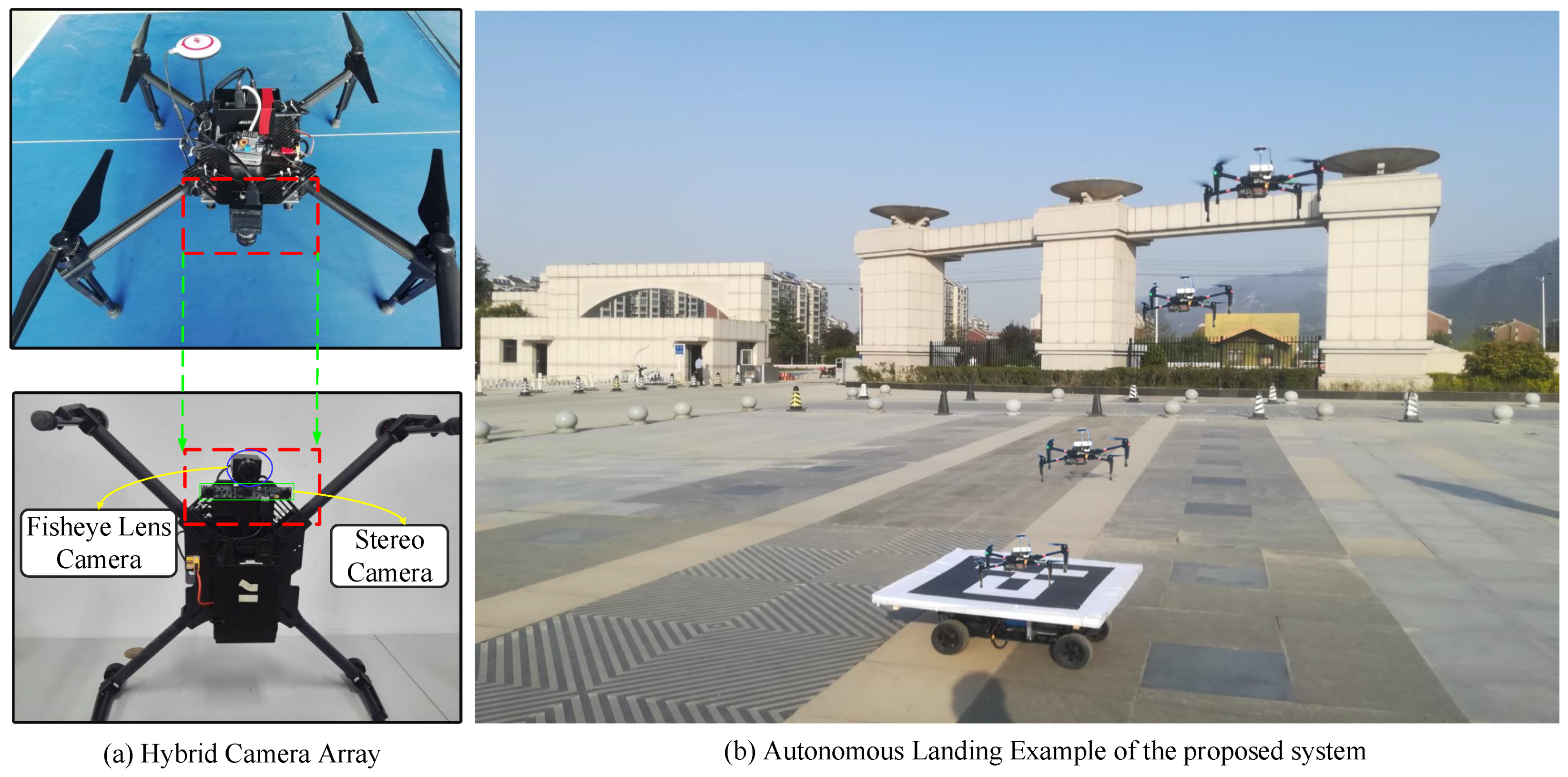
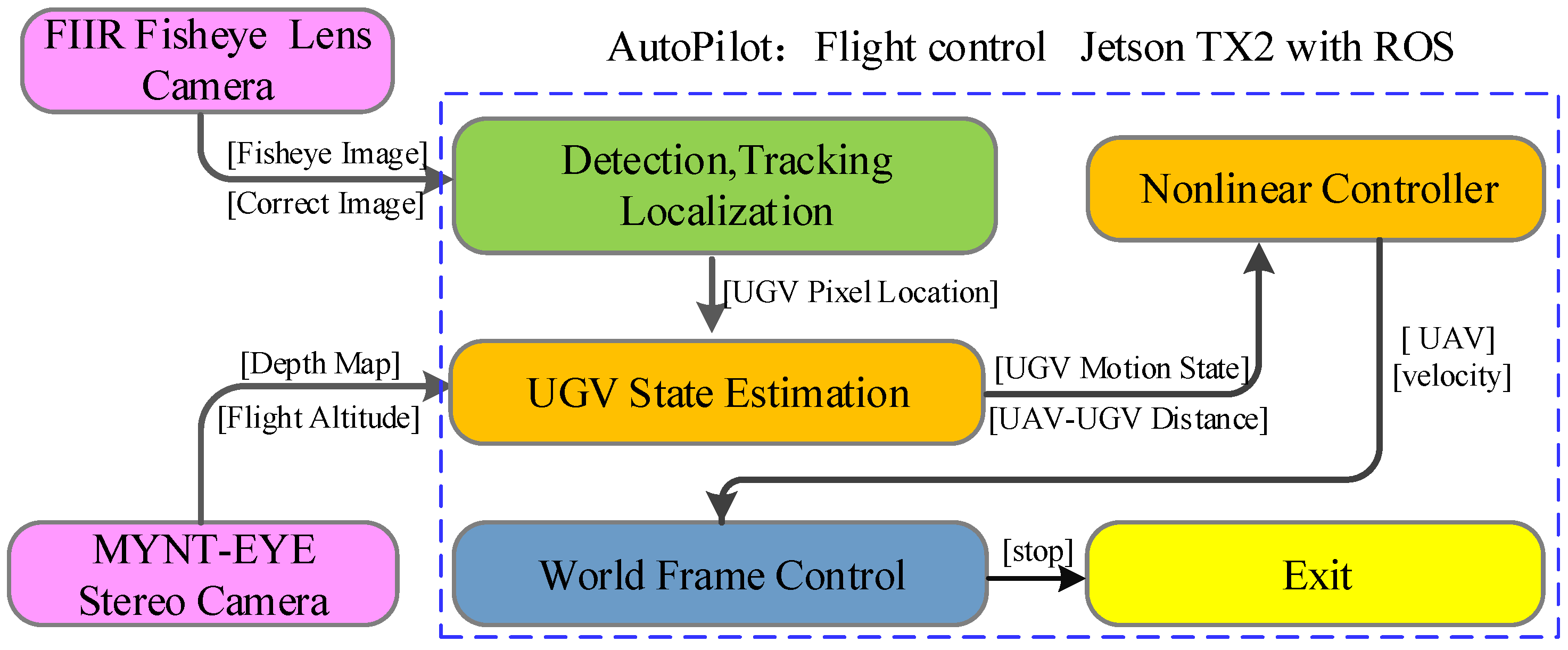
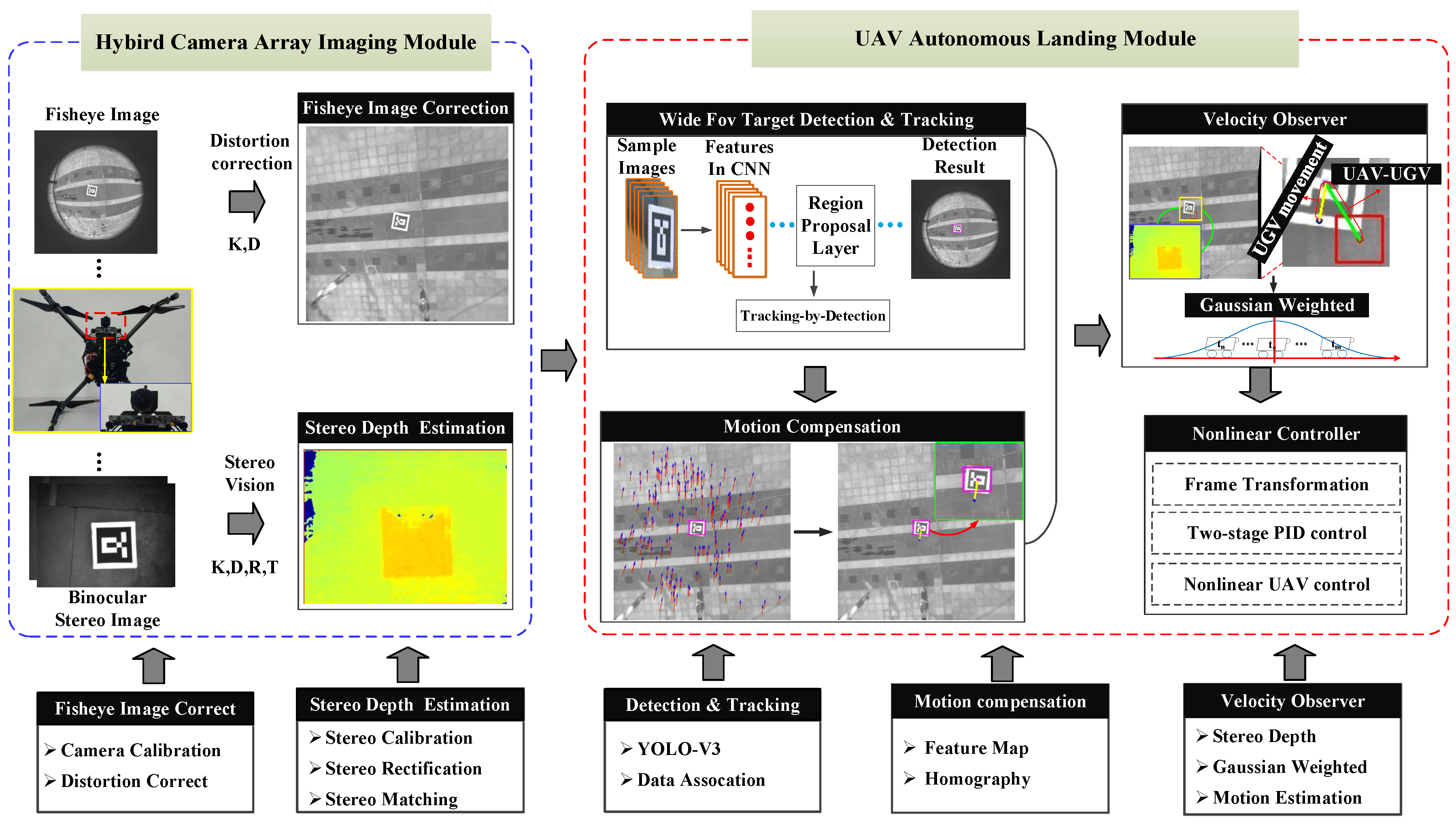
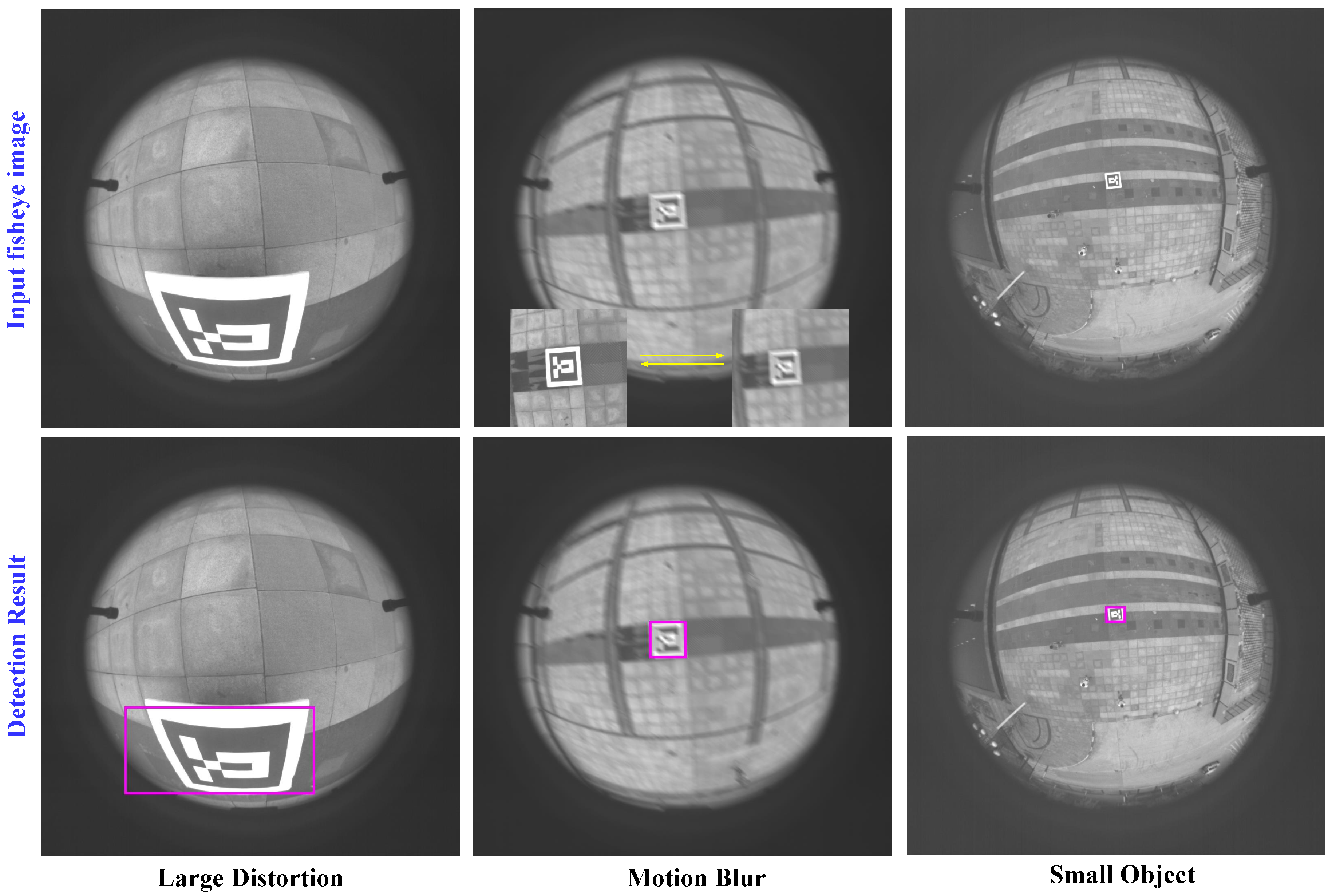
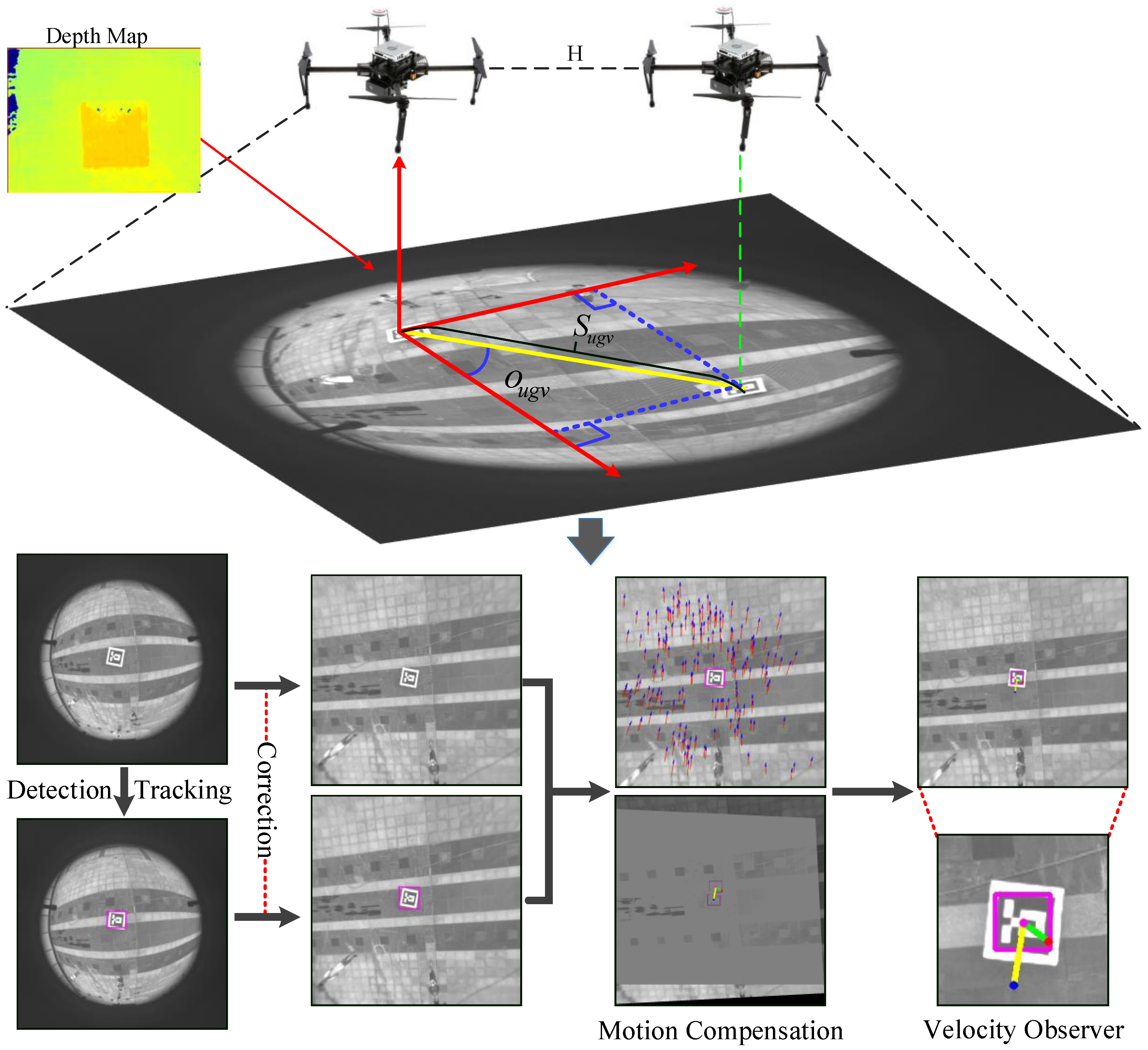
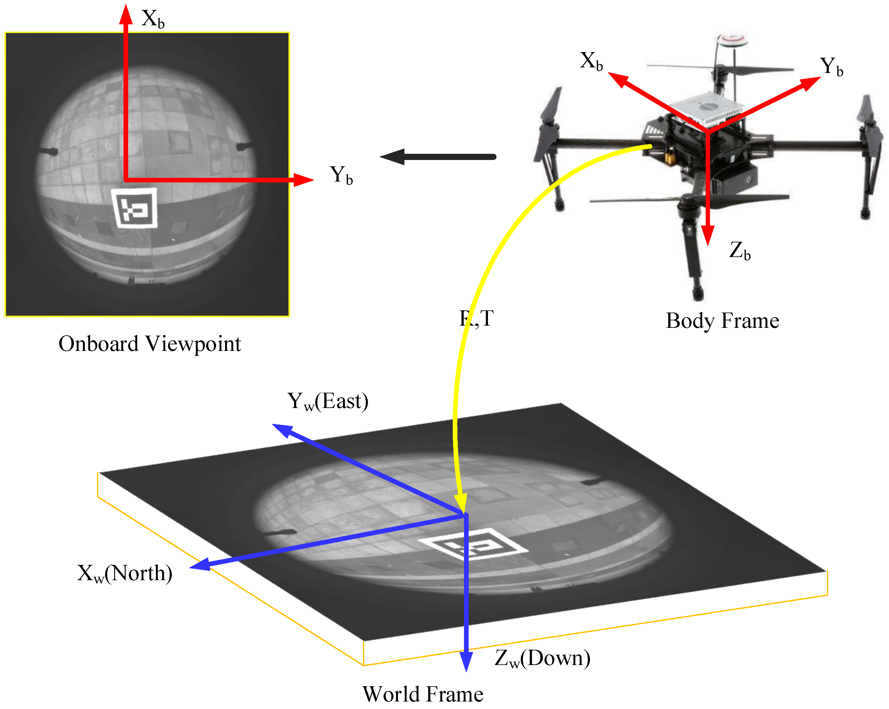
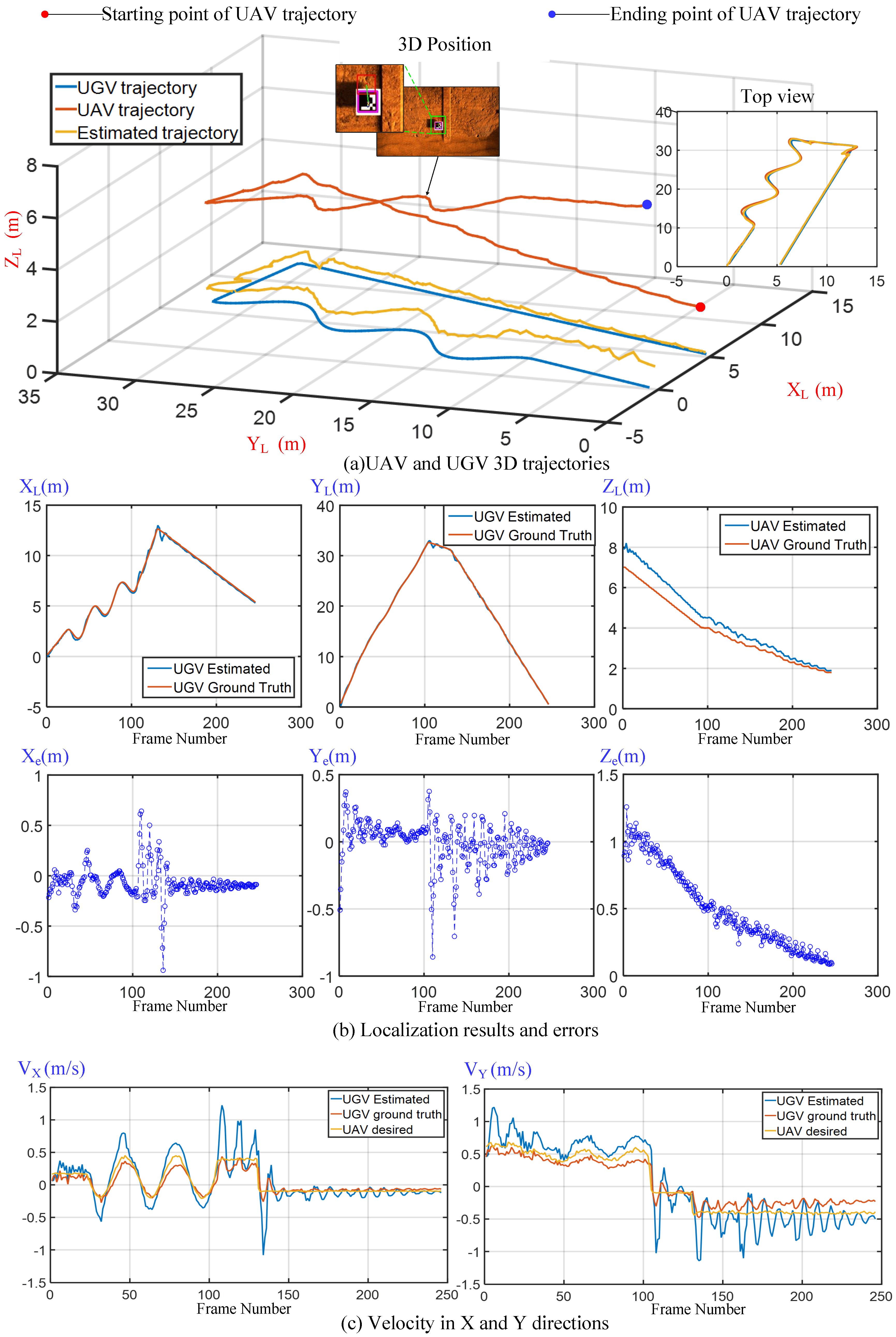
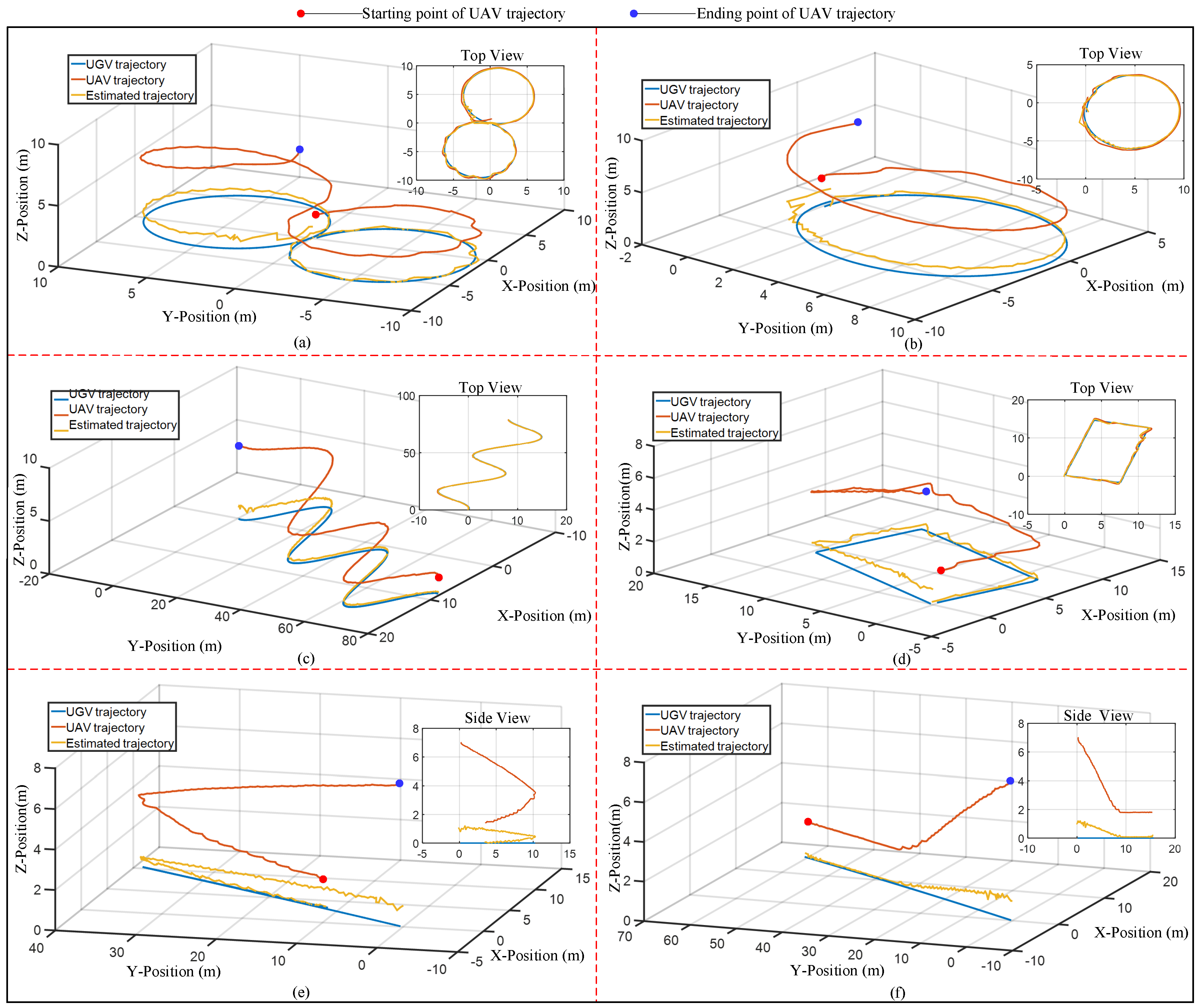
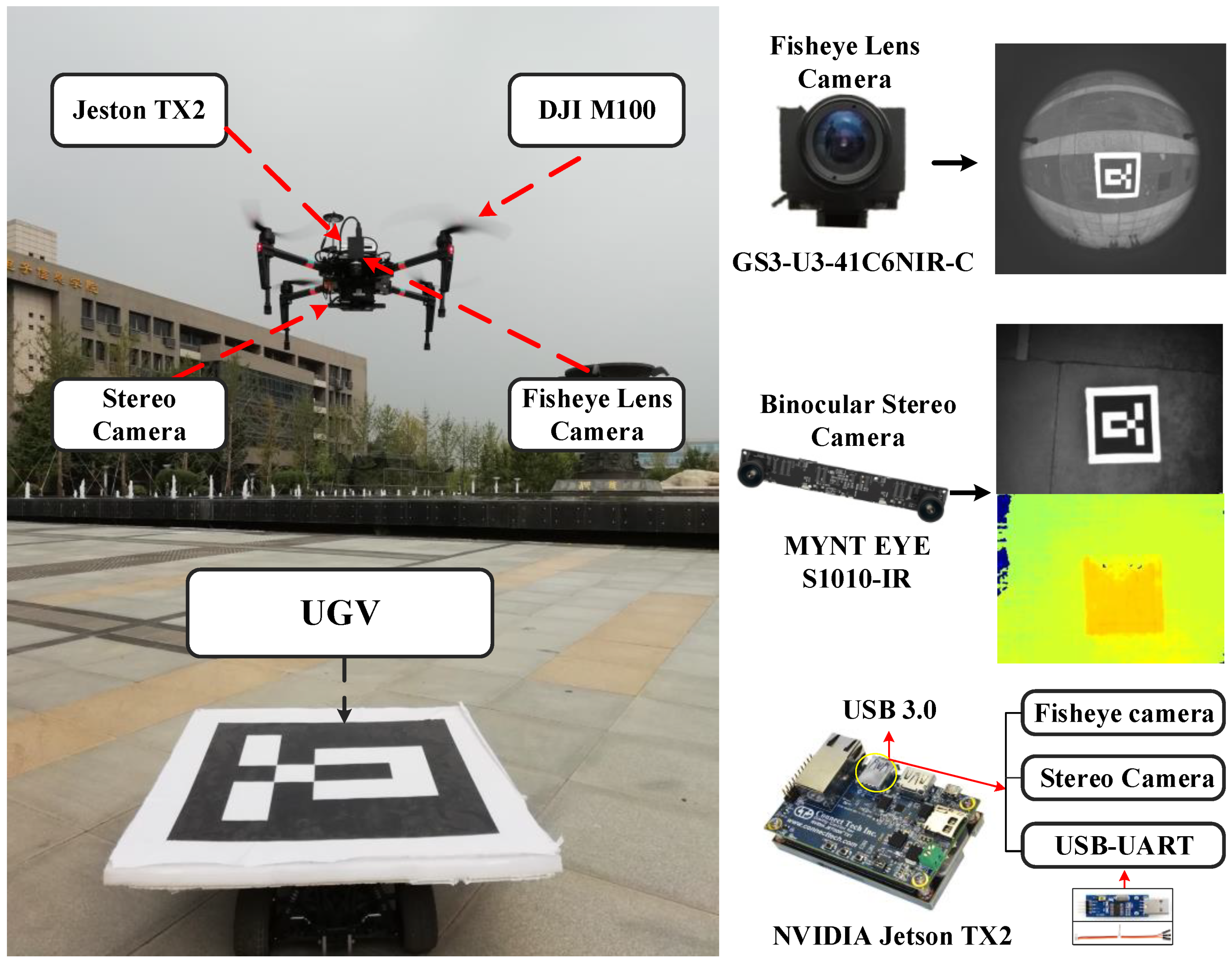
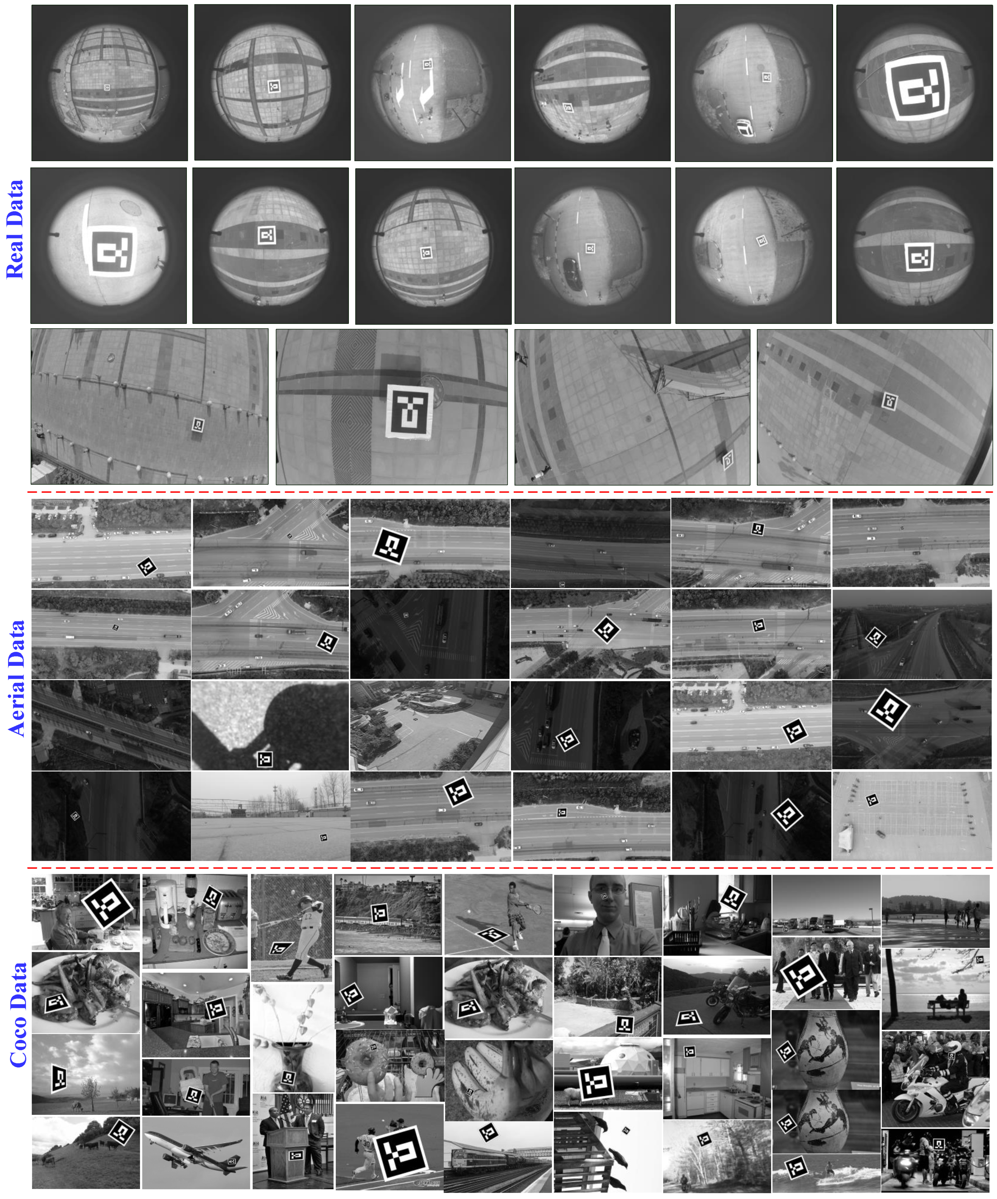
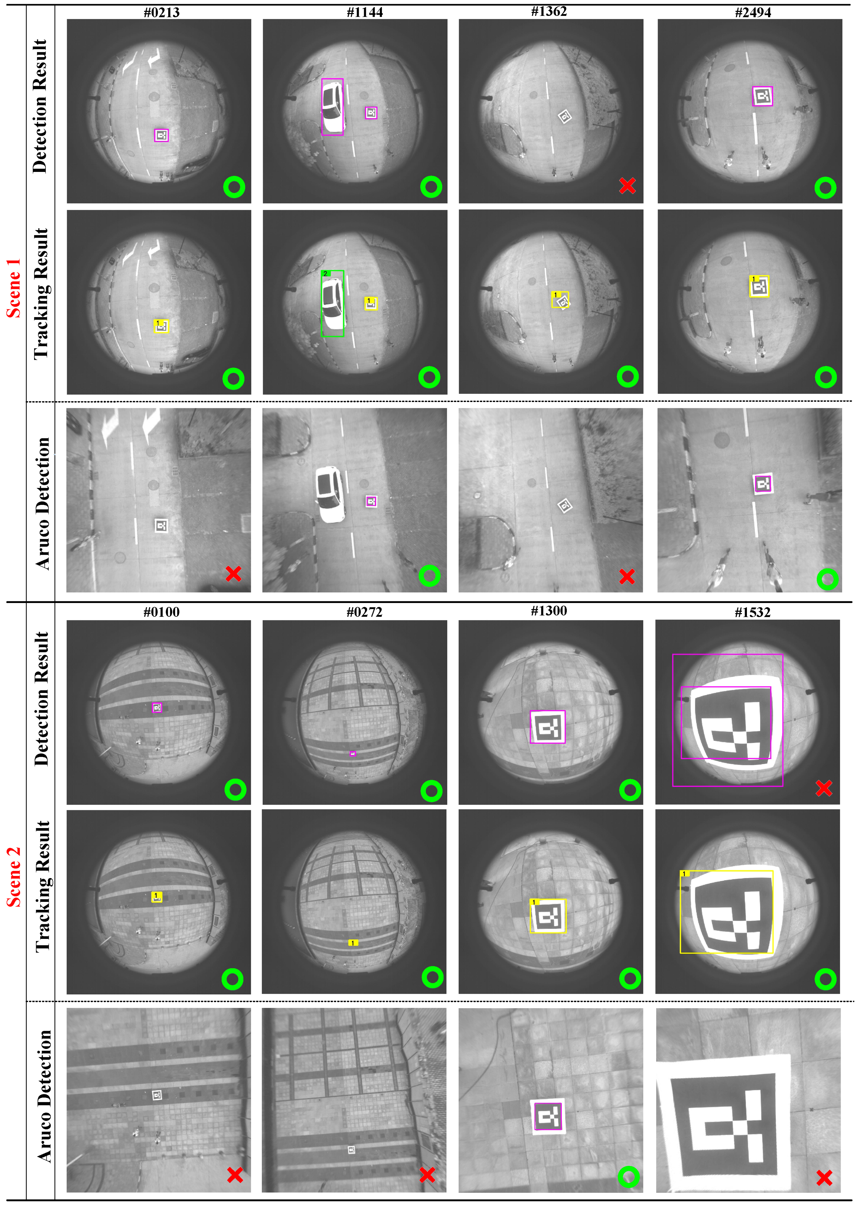
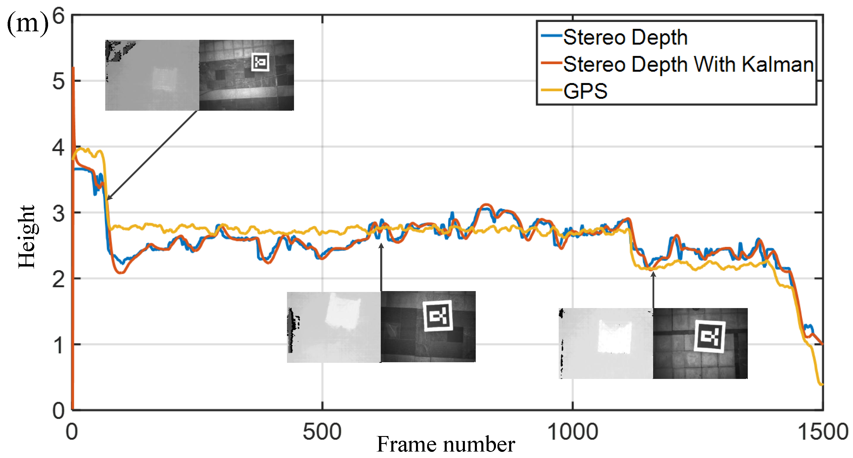
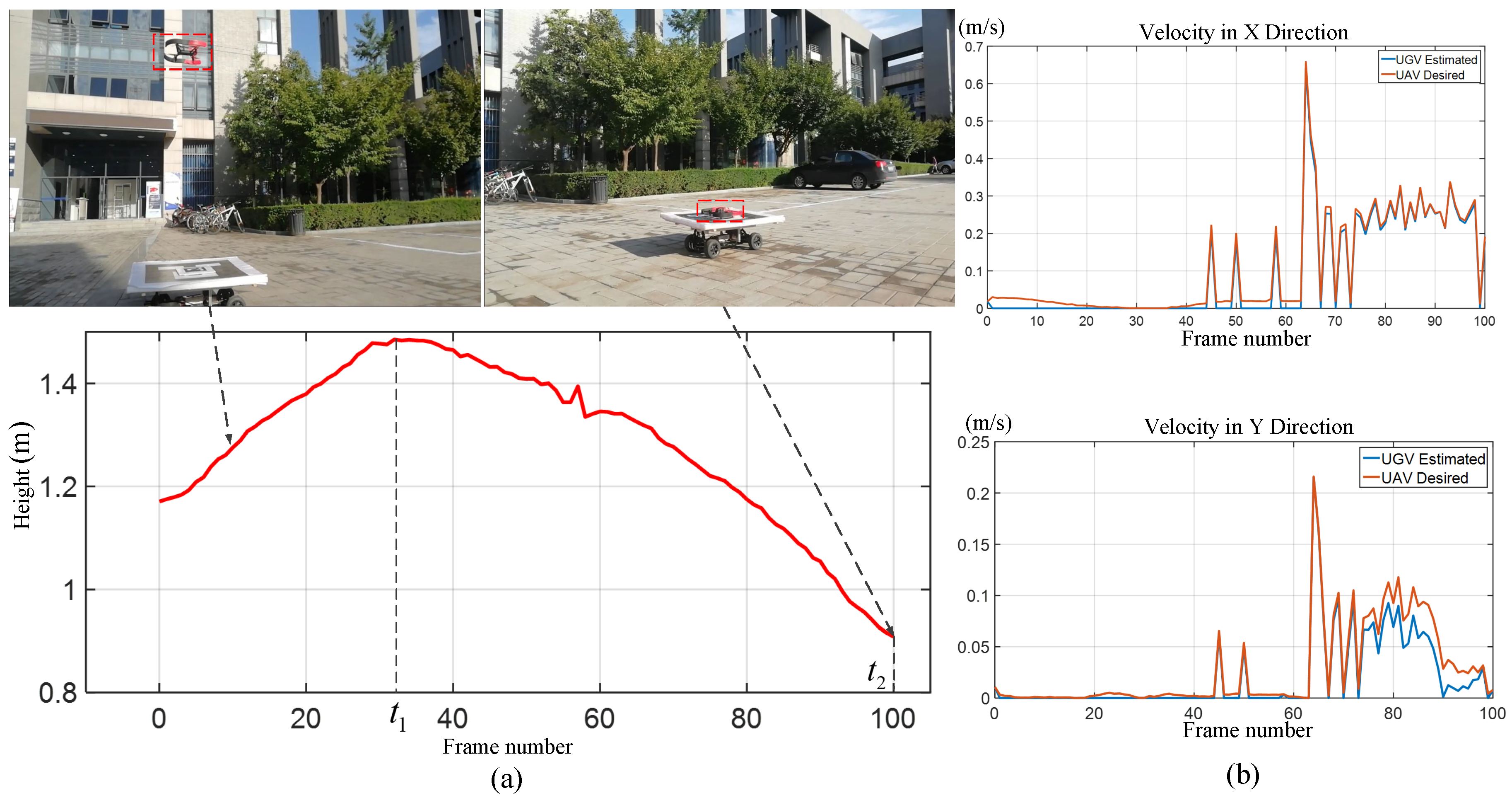
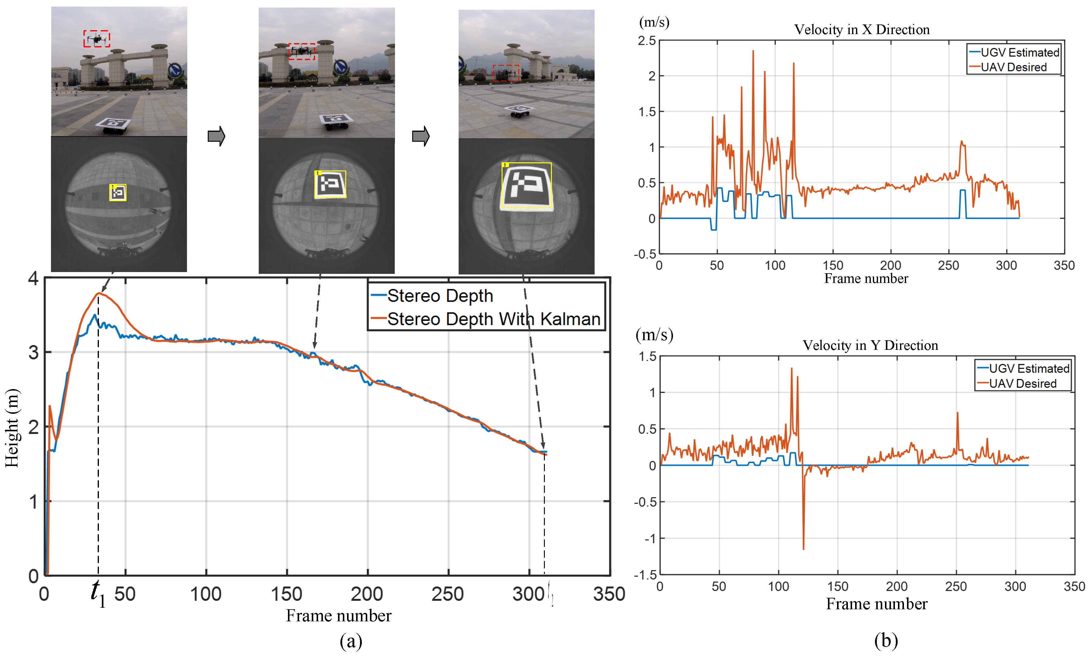
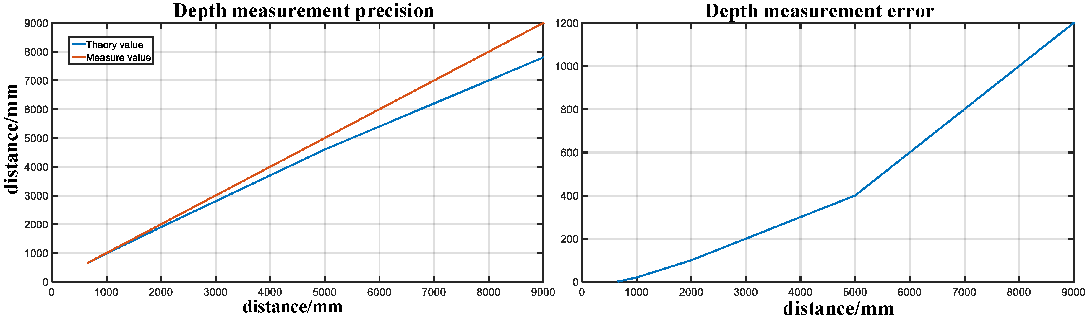
Table 1.
The camera and lens parameters.
| Camera/Lens | Specification | Parameter |
|---|---|---|
 | Sensor | CMV4000-3E12 |
| Resolution | pixels | |
| Frame rate | 90 fps | |
| Interface | USB 3.0 | |
| Power consumption | 4.5 W | |
| Infrared Camera | Operating temperature | C to ∼50 C |
 | Focal length | 3.5 mm |
| Angle of View | ||
| Magnification | ||
| TV distortion | % | |
| Kowa LM4NCL | Compatible sensor | 1.1 |
 | Focal length | 2.1 mm |
| Resolution | ||
| Base line | 120.0 mm | |
| Frame rate | 60 fps | |
| Interface | USB 3.0 | |
| Power consumption | 3.50 W | |
| MYNT EYE S1030-IR | Operating temperature | C to ∼40 C |
Table 2.
The PID control parameters.
| Experiments | Height (m) | |||
|---|---|---|---|---|
| Simulation | ≥4 | 0.80 | 0.00 | 0.35 |
| <4 | 1.50 | 0.00 | 0.50 | |
| Real-World (DJI) | ≥3 | 0.50 | 0.00 | 0.20 |
| <3 | 0.70 | 0.00 | 0.25 |
Table 3.
The detection performance on the test dataset.
| Datasets | Total Targets | TP | FP | FN | Precision | Recall | F1-Measure |
|---|---|---|---|---|---|---|---|
| Scene 1 | 408 | 391 | 0 | 17 | 100.00% | 95.83% | 97.87% |
| Scene 2 | 960 | 957 | 0 | 3 | 100.00% | 99.68% | 99.83% |
| Scene 3 | 934 | 932 | 0 | 2 | 100.00% | 99.78% | 99.88% |
| Scene 4 | 421 | 419 | 0 | 2 | 100% | 99.52% | 99.75% |
| Scene 5 | 3175 | 3175 | 2 | 0 | 99.93% | 100.00% | 99.96% |
| Total | 5898 | 5874 | 2 | 24 | 99.62% | 99.59% | 99.60% |
Table 4.
The NVIDIA Jetson TX2.
| Content | Jetson TX2 |
|---|---|
| GPU | NVIDIA Pascal, 256 CUDA cores |
| CPU | dual-core NVIDIA Denver2 + quad-core ARM Cortex-A57 |
| Memory | 8 GB 128-bit LPDDR4 59.7 GB/s |
| PCIE | Gen 2 | 1 × 4 + 1 × 1 OR 2 × 1 + 1 × 2 |
| USB | USB 3.0 + USB 2.0 |
| Mechanical | 50 mm × 87 mm (400-Pin Compatible Board-to-Board Connector) |
Table 5.
The CPU usage in NVIDIA Jetson TX2.
| Core 1 | Core 2 | Core 3 | Core 4 | Core 5 | Core 6 |
|---|---|---|---|---|---|
| 43–66% | 65–99% | 57–98% | 43–62% | 40–62% | 41–69% |
Table 6.
The YOLOv3-416 compared to YOLOv3-tiny in NVIDIA Jetson TX2.
| Model | Train | Test | Speed (FPS) | Precision | Recall | F1-Measure |
|---|---|---|---|---|---|---|
| YOLOv3-416 | UGV_Train_Data | Scene 5 | 3.00 | 98.91% | 100.00% | 99.45% |
| YOLOv3-tiny | UGV_Train_Data | Scene 5 | 20.00 | 99.93% | 100.00% | 99.96% |
Table 7.
The Computation time for Jetson TX2.
| Content | Mean | Standard Deviation | |
|---|---|---|---|
| Fisheye Correction | 6.15 | 1.97 | (ms) |
| Stereo Depth Estimation | 23.77 | 2.66 | (ms) |
| Detection | 51.24 | 55.69 | (ms) |
| Tracking | 1.51 | 0.86 | (ms) |
| Motion compensation | 105.71 | 0.03 | (ms) |
| Nonlinear Control | 0.34 | 0.07 | (ms) |
| Total (Max thread) | 110.08 | 0.03 | (ms) |
© 2018 by the authors. Licensee MDPI, Basel, Switzerland. This article is an open access article distributed under the terms and conditions of the Creative Commons Attribution (CC BY) license (http://creativecommons.org/licenses/by/4.0/).
Share and Cite
MDPI and ACS Style
Yang, T.; Ren, Q.; Zhang, F.; Xie, B.; Ren, H.; Li, J.; Zhang, Y. Hybrid Camera Array-Based UAV Auto-Landing on Moving UGV in GPS-Denied Environment. Remote Sens. 2018, 10, 1829. https://0-doi-org.brum.beds.ac.uk/10.3390/rs10111829
AMA Style
Yang T, Ren Q, Zhang F, Xie B, Ren H, Li J, Zhang Y. Hybrid Camera Array-Based UAV Auto-Landing on Moving UGV in GPS-Denied Environment. Remote Sensing. 2018; 10(11):1829. https://0-doi-org.brum.beds.ac.uk/10.3390/rs10111829
Chicago/Turabian StyleYang, Tao, Qiang Ren, Fangbing Zhang, Bolin Xie, Hailei Ren, Jing Li, and Yanning Zhang. 2018. "Hybrid Camera Array-Based UAV Auto-Landing on Moving UGV in GPS-Denied Environment" Remote Sensing 10, no. 11: 1829. https://0-doi-org.brum.beds.ac.uk/10.3390/rs10111829
Note that from the first issue of 2016, this journal uses article numbers instead of page numbers. See further details here.