Towards a 20 m Global Building Map from Sentinel-1 SAR Data


Luxembourg Institute of Science and Technology (LIST), Environmental Research and Innovation Department (ERIN), 4422 Belvaux, Luxembourg
*
Author to whom correspondence should be addressed.
Remote Sens. 2018, 10(11), 1833; https://0-doi-org.brum.beds.ac.uk/10.3390/rs10111833
Submission received: 17 September 2018
/
Revised: 28 October 2018
/
Accepted: 10 November 2018
/
Published: 19 November 2018
(This article belongs to the Special Issue Classification and Feature Extraction for Remote Sensing Image Analysis)
Abstract
:This study introduces a technique for automatically mapping built-up areas using synthetic aperture radar (SAR) backscattering intensity and interferometric multi-temporal coherence generated from Sentinel-1 data in the framework of the Copernicus program. The underlying hypothesis is that, in SAR images, built-up areas exhibit very high backscattering values that are coherent in time. Several particular characteristics of the Sentinel-1 satellite mission are put to good use, such as its high revisit time, the availability of dual-polarized data, and its small orbital tube. The newly developed algorithm is based on an adaptive parametric thresholding that first identifies pixels with high backscattering values in both VV and VH polarimetric channels. The interferometric SAR coherence is then used to reduce false alarms. These are caused by land cover classes (other than buildings) that are characterized by high backscattering values that are not coherent in time (e.g., certain types of vegetated areas). The algorithm was tested on Sentinel-1 Interferometric Wide Swath data from five different test sites located in semiarid and arid regions in the Mediterranean region and Northern Africa. The resulting building maps were compared with the Global Urban Footprint (GUF) derived from the TerraSAR-X mission data and, on average, a 92% agreement was obtained.
1. Introduction
Land cover and its changes have a significant impact on society, with effects such as the alteration of water and energy exchanges between the earth surface and the atmosphere, and changes in the sources of greenhouse gases and aerosols, as well as their decline. Moreover, land cover distribution is partially influenced by the regional climate. Hence, changes in land cover are an important element to consider when assessing climate change and its impacts [1]. In this context, land cover at a global scale is an essential variable for understanding the multiple relations between human activities and global change [2]. One important class of land cover is represented by urban areas that have a particularly strong effect on a region’s climate [3]. In most regions, the urban areas only represent a relatively small fraction of the overall land cover. However, in spite of their rather limited coverage worldwide, the detection and analysis of their extent, the estimation of population density, and the monitoring of population migration are all prerequisites for accurately assessing the impact of human activities on the environment [4]. Further evidence of this is provided in the 2014 United Nations World Urbanization Prospects report stating that 54% of the world’s population resides in urban areas and that this percentage is expected to increase to 66% by 2050 [5]. Observations from space can provide unique and much-needed information that enables a better understanding of the evolution of built-up areas and a more successful management of climate change. To this aim, many initiatives have been launched to generate high-precision land cover maps at a global scale that are based on different sensor data and made available at different spatial resolutions. In this context, the European Space Agency (ESA) has undertaken the Climate Change Initiative program to respond to the need for climate data of different organizations, such as the United Nations Framework Convention on Climate Change (UNFCCC) and the Global Climate Observing System (GCOS). In this context, one of the Essential Climate Variables (ECVs) is the global land cover map, which is provided at a resolution of 300 m. Some classes, such as water bodies, come at a higher resolution (up to 150 m) [6]. Regarding product needs for change analyses of urban areas, it was highlighted in a GCOS report [1] that land cover maps scales of 10–30 m should be produced annually.
Presently, global land cover maps are obtained using optical satellite data with a resolution ranging from 30 m (using optical Landsat Thematic Mapper (TM) and Enhanced Thematic Mapper Plus (ETM+) data) [2] to 500 m (using Modis data) [7]. Generating land cover inventories was the main scope of the early spaceborne missions focusing on the observation of our planet.
Synthetic aperture radars (SARs) are rarely the primary source of information for land cover classification, especially when multispectral optical images at high spatial resolution are available [8,9,10,11,12]. SAR data are more often used merely as a complementary or alternative data source in case of unfavorable atmospheric conditions or to identify classes that have a highly distinctive scattering behavior. Two good examples are (1) calm/shallow water, which is typically characterized by very low backscattering due to the specular reflection on very smooth surfaces, and (2) buildings, for which the appearance of double-bounce effects results in a drastic increase in the backscattering due to the presence of dihedral structures. It is the focus of this paper, therefore, to map building areas.
SAR images have several limitations in terms of information content when compared to optical ones, mainly due to the limited number of spectral channels available. Generally, a single frequency and one polarization are employed in classical SAR sensors. However, some of the SAR sensors also have dual and quad-polarization modes. Moreover, SAR images are affected by a peculiar noise, namely, the speckle, which is known to deteriorate the radiometric resolution, thereby influencing any classification step. In order to classify built-up areas using SAR data, textural parameters have been frequently used to attenuate the speckle effect and cope with the lack of information content [13]. Textural features, often in combination with multi-temporal datasets, have shown some potential to distinguish between different urban densities, as well as different types of urbanization [14]. Usually, given the multiscale nature of urban environments, the textural features are derived in a multiscale manner to overcome the limitations of single-scale procedures [15]. The use of supervised Bayesian classification methods based on the combination of textural features and amplitude derived from very high resolution SAR images has been promising for mapping urban areas [16]. Moreover, the SAR intensity was coupled with the interferometric phase extracted from two very high resolution SAR images to detect building edges [17]. Multi-temporal interferometric coherence represents another characteristic element that can be relevant for detecting urban areas. SAR coherence is defined as the correlation between the complex images of an interferometric image pair and thus provides information about the temporal steadiness of classes (i.e., coherence). As urban areas are likely stable over time intervals, the coherence can be used for delineating building footprints [18]. In [19], interferometric coherence information was used in order to detect human settlements from Sentinel-1 images. Polarimetric SAR data have also shown some promise for classifying urban areas thanks to their ability to identify the double-bounce component of the scattering when building facades are aligned with the satellite’s flight direction or to identify rotated dihedrals using the cross-polarization channel. Indeed, by making use of polarimetric information, it is even possible to determine the orientation of building facades with respect to the SAR’s line of sight [20]. As shown in Stasolla and Gamba [21], autocorrelation indices extracted from SAR intensity can be used to identify regular patterns, including those corresponding to urban areas. The spatial distribution of bright pixels has also been exploited to map buildings using a region-growing approach that employs a filtered multi-temporal average of a SAR intensity time series of Envisat ASAR data, acquired in Wide Swath Mode (WSM), with a spatial resolution of 150 m [22]. Recently, the same technique was also applied and validated with Sentinel-1 data [23]. The KTH-Pavia Urban Extractor, applied to C-band ASAR VV data, showed its effectiveness in detecting built-up areas at a 30 m resolution with very good accuracy [24]. This result indicates that urban mapping at a large scale is possible with spaceborne SAR data, especially when considering the large collections of Sentinel-1 (S-1) data that are available today. This method has been applied to 10 major cities and one rural area, as well as to smaller towns on six continents, showing its capability for mapping buildings in both urban and rural areas. It makes use of spatial indices and texture features, in addition to multi-temporal information [25].
The first so-called Global Urban Footprint (GUF) product is a binary settlement map at an unprecedented high spatial resolution of 12 m. It was derived using SAR data recorded by the TanDEM-X and TerraSAR-X X-band radar sensors. It provides a global-scale map of urban and rural settlements and was derived by means of a fully automated processing framework that analyzes an archive of more than 180,000 images with a spatial resolution of 3 m collected between 2011 and 2012 [26]. The approach consists of applying an unsupervised classification procedure to the backscatter amplitude data and to the speckle divergence, the latter being considered a measure of texture. A post-processing filtering operation is applied to the classification result and makes use of a set of reference layers providing different types of information, such as relief mask, road cluster, water body maps, or the Copernicus imperviousness layer.
As seen from the literature review, the potential for using SAR data to map urban areas has been assessed in multiple studies. These methods are of high interest due to the capability of the S-1 C-band SAR mission to systematically acquire images with a large swath width (i.e., 240 Km) and high spatial resolution (i.e., 20 m) in the Interferometric Wide Swath (IW) acquisition mode. In this context, on 1 September 2015, the ESA CCI-LC initiative launched an Urban Round-Robin (RRob) exercise. The aim of the RRob activity was the selection and identification of the most efficient algorithm for improving/updating the existing global urban land cover products using S-1 data. It is in this framework that we developed an automatic algorithm that exploits the multi-temporal interferometric coherence and the temporal information content of both the co- and cross-polarization channels of the S-1 SAR data in order to generate building maps at a 20 m resolution. The algorithm proposed makes use of a hierarchical split-based approach (HSBA) method to parameterize the distribution functions of the classes of interest [27,28]. Subsequently, based on the class distributions, a building map is generated using a hybrid SAR-based methodology that consists of a sequence of region-growing and histogram thresholding processes [27,29].
2. Methodology
2.1. SAR Feature Extraction and Algorithm Architecture for Identifying Buildings
SAR co-polarization backscattering, HH and VV, in urban areas is influenced by the double-bounce effect caused by the presence of buildings. The double-bounce is represented by the facade–ground and ground–facade scattering. Moreover, as double-bounce ray paths all have the same length, equal to the distance between the SAR sensor and the facade base illuminated by the radar, a high-value of backscattering is recorded. The double-bounce backscatter is composed of a coherent contribution (scattering from a dihedral reflector) and an incoherent one. The latter depends on the surface roughness, which can be defined with a Gaussian-type autocorrelation function. In urban areas, the coherent reflection dominates since the walls and streets can be considered smooth surfaces with respect to the signal wavelengths, such as those in the X, C, and L bands. Considering the angle between the satellite flight direction and the intersection line of the wall and road, the backscattering is at its maximum at 0 and declines gradually for higher angles [30,31,32]. To increase the possibility of detecting this type of behavior, it is useful to consider more than one azimuth looking angle. In urban areas, the building topology may substantially vary from one settlement to another, depending on the density of the urban fabric, the orientation of the buildings, the street width, etc. All these factors influence the double-bounce effect. Consequently, combining images of the same area from both ascending and descending orbits allows two lines of sight of the same building to be exploited, thereby increasing the chance to identify the effect of the double-bounce mechanism. For buildings with gable roofs, the part of the roof that is oriented toward the sensor produces a foreshortening effect that is an additional direct contribution to the backscattering [33,34]. This feature is another example where the joined use of ascending and descending images helps improve the characterization of buildings as objects generating high backscattering.
An additional important source of information that could be helpful for detecting buildings is cross-polarization backscattering (VH/HV). As stated by Sato et al. [35], the cross-polarization component increases due to multiple-bounce in the presence of more complex structures, such as oriented building blocks, i.e., the ones where the façade is not aligned with the satellite flight direction. However, the cross-polarization backscattering also increases due to volumetric scattering caused by the presence of vegetation. This could thus potentially produce false alarms. The same type of problem may occur for the co-polarization channel, where the typology of vegetation, especially with vertical stems, causes a significant increase in backscattering values.
To cope with problems of false alarms generated by vegetated areas, we propose employing the multi-temporal InSAR coherence, . Indeed, when assessing temporal coherence, one may consider that vegetation and buildings exhibit opposite behaviors. Buildings are considered stable structures while vegetated areas are not [36]. The complex coherence is primarily influenced by the phase difference between radar returns, the latter being a distinctive parameter measured by coherent sensors, such as SARs. Moreover, is particularly sensitive to the spatial arrangement of the scatterers within a pixel cell and thus to their possible random displacements. As stated in Zebker and Villasenor [37], factors that can influence InSAR coherence and that are sources of decorrelation are the spatial baseline, the rotation of the target between observations, and the temporal decorrelation. It is evident that these factors are the ones enabling the distinction between man-made structures and vegetated areas, while the spatial baseline, on the contrary, can attenuate this difference. The increase in the spatial baseline, particularly its perpendicular component, implies a decrease in the coherence, thus reducing the value of this feature for discriminating classes as coherent and incoherent in time [38]. The effect of the perpendicular baseline is even more important in urban areas where the geometrical complexity of structures accentuates this effect [34]. Concerning this last aspect, the S-1 mission is suitable for providing reliable coherence maps, given that the spatial baseline between image pairs is always limited and, in the worst case, equals 100 m. Hence, the decrease in coherence due to the perpendicular baseline is significantly reduced.
Based on the above-mentioned considerations, buildings imaged by a SAR sensor with a resolution in the order of tens of meters appear significantly brighter than other land cover classes in both the co- and cross-polarization intensity channels; at the same time, buildings show high values of multi-temporal InSAR coherence. However, steep slopes facing the sensor can also exhibit high backscattering values in SAR images due to the foreshortening effect [39]. When such areas are scarcely vegetated, the coherence values are also high. For these reasons, the detection of buildings under these circumstances may be problematic. To cope with this issue, it is highly recommended to make use of a digital elevation model (DEM) to determine areas where the foreshortening occurs [40]. In this study, we used the local incidence angle (LIA) derived from the SRTM30m DEM to identify steep slopes as pixels with markedly different values compared to the incidence angle computed based only on the ellipsoid. Based on a thresholding operation that verifies whether the difference between the two aforementioned incidence angles is higher than 90, foreshortening, layover, and shadow areas can be easily identified [39].
When handling SAR data, it is worth pointing out the importance of accounting for speckle noise, which generally hampers image classification using only backscattering values at the pixel level. Indeed, many approaches dealing with the urban area classification problem make use of textural features or efficient extractors that rely more on the spatial arrangement of pixels than the pixels themselves [14,41,42,43]. Usually, these approaches reduce the resolution of the produced maps because the parameters are derived using spatial filtering with a kernel of a certain size. Another common and simple operation that reduces the speckle effect is to create a multi-look image, which has the same drawback of decreasing the spatial resolution, thereby hampering the full exploitation of the high spatial resolution that SAR sensors offer. Temporal averaging represents an appropriate filtering approach when a temporal series of images are available. Its main advantage is that, contrary to the multi-looking and textural approaches, it reduces the speckle without decreasing the spatial resolution, making it well-suited for the classification of smaller (with respect to the resolution of the sensor) objects. It is supposed that a building is present in the entire time series, thus, the corresponding pixel is homogeneous in time. However, if another land cover class is present before or after, the pixels may be wrongly classified because the averaging operator can diminish the backscattering value. This drawback can be attenuated, reducing the time span of the time series, although it can be advantageous to analyze the vegetation classes that show a high backscattering value just for a certain period of the year. The long time period average can decrease the mean value of vegetation classes, increasing the separability between buildings and vegetation. A typical example is rice fields, which show high backscattering values in certain periods of the year, and very low ones in others [44]. The S-1 mission is particularly well-suited for applying this kind of filtering, as it systematically acquires images with a high revisit time (6 days). This makes it possible to generate building maps at the native sensor resolution, with a temporal resolution of a few months, while at the same time providing the possibility to average a sufficiently long time series of images. Hence, taking advantage of the S-1 mission characteristics, here, we propose an algorithm that is based on the following features:
- (a)
- Temporal average intensity (TAI) VV-ASC & -DESC ( and ): for these features, we average a multi-temporal set of co-polarization SAR intensity images. Both ascending and descending orbits are considered separately, and the two corresponding features will be employed for identifying buildings, i.e., areas of high backscattering. Both features are derived for the co-polarization SAR images knowing that this configuration is favorable for detecting the double-bounce effect that is usually observed in urban areas.
- (b)
- TAI VH-ASC & -DESC ( and ): these features are obtained as in (a) but we consider the cross-polarization channel, which is better suited for detecting buildings with a dihedral shape that are not perfectly aligned with the orbit orientation.
- (c)
- Temporal average coherence (TAC) VV-ASC & -DESC ( and ): the multi-temporal coherence is derived by averaging the coherences extracted from the successive interferometric image pairs of the multi-temporal set. The computation is made for both ascending and descending orbits while only the co-polarization channel is considered.
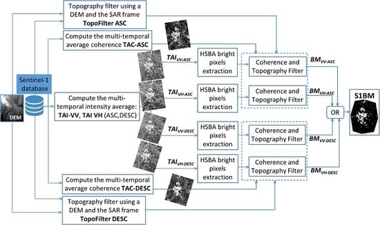
Based on the above-mentioned input features, the algorithm is composed of the following steps, illustrated in the block diagram given in Figure 1:
- (i)
- Identify double-bounce objects, i.e., brighter pixels, in all four temporally averaged intensities (, , , and ) using a hierarchical split-based thresholding approach (HSBA), which is described in the following subsection.
- (ii)
- From the binary maps generated using step (i), remove all pixels that show low coherence values according to the two averaged coherence maps obtained from the temporal series of ascending and descending orbits, and .
- (iii)
- Remove all pixels in mountainous areas potentially affected by foreshortening for ascending or descending orbits, respectively.
- (iv)
- Merge the four separate resulting buildings maps, , , , and , to obtain the final S-1 Buildings Map (S1BM).
2.2. Identification of Bright Pixels in the Co- and Cross-Polarization SAR Channels
In any given SAR intensity image, three canonical scattering mechanisms can be distinguished: (i) surface scattering, where the energy is scattered or reflected from a well-defined interface; (ii) volume scattering, where a single scattering site is not identifiable, as the reflections come from several elements (e.g., components of a tree canopy); (iii) hard-target scattering, such as corner/dihedral reflector behavior, which produces high responses in terms of backscatter. In reality, more than one scattering mechanism may simultaneously occur within a given pixel [45]. The strength of surface scattering depends on surface roughness and the dielectric constant of the scattering material. Considering water as a singular surface with a high dielectric constant and a very smooth surface in the absence of wind, it behaves as a typical specular reflector at radar wavelengths, causing low values of recorded backscattering; on the other hand, we can associate buildings with the hard-target scattering mechanism, typically characterized by high backscattering values and a distribution that is easily distinguishable from all other classes. The remaining land cover classes are characterized by both volume and surface scattering mechanisms, resulting in backscattering values between those of the two previously described classes. It follows that two main classes, namely, water and buildings, can be extracted from the backscatter distribution derived from a single SAR intensity image with both cross- and co-polarizations. These two classes are positioned in the lower and upper parts of the backscattering values histogram, respectively. In this study, and considering this assumption, we targeted the mapping of the building class.
Accurate classifications require adequate training data and parameter settings. When the objective is to classify just one class, conventional supervised classifiers are arguably not the best choice, since all classes have to be exhaustively defined in the training step of the analysis [46]. Conversely, one-class classifiers (OCCs) represent a relevant option because a training dataset is only necessary for the class of interest, i.e., positive samples, while, for all other classes, i.e., unlabeled samples, training data are not compulsory. Moreover, the OCCs can be separated into two main categories: the P-classifiers that make use only of positive samples as the training dataset and the PU-classifiers that consider both positive and unlabeled samples. PU-classifiers are computationally more demanding than P-classifiers, since a significant number of unlabeled samples are usually required as input. On the other hand, they tend to yield more accurate results, especially when positive and unlabeled classes overlap. To derive a binary classification, a threshold has to be applied and, especially for an OCC PU-classifier, its selection may be rather difficult [47,48].
To select the best threshold, here we used an adaptive approach that was originally developed as an algorithm for mapping water bodies [27,28,29]. The algorithm is statistically based and makes use of a hierarchical tilling of the image in order to define the probability density function (PDF) of the class of interest. Once the PDF of the class of interest has been estimated, the algorithm combines histogram thresholding and region-growing processes to identify the class of interest. The proposed approach can be associated with the OCC PU-classifier family since it attempts to characterize the positive and unlabeled samples in the training phase. The parameters of the region-growing and thresholding processes are automatically derived from the previously calibrated PDF of the class of interest (positive samples), i.e., Building Class (BC), and the one that represents the other pixels (unlabeled samples), i.e., all Other Classes (OC). The definition of the PDF for the BC is only possible if the class itself is identifiable, and this generally depends on the shape of the histogram. The BC may not be easily identifiable from the histogram in the common case when buildings represent only a small percentage of the entire image. Therefore, it is necessary to focus on those areas of the image that are, to a certain extent, composed of a similar number of pixels belonging to the BC and OC, respectively. For this reason, here we used an HSBA [27] to automatically identify regions in any given SAR image where the PDF of the BC is well-separated from that of the OC, and both have similar coverage. The objective is thus to obtain a robust parameterization of the BC and OC PDFs, which, in turn, can then be used to achieve a more accurate and reliable classification of the class of interest. Here, the PDFs of the BC and OC are assumed to be Gaussian. This choice is motivated by the fact that the input data are multi-looked, log-transformed SAR intensity images and averaged over time to increase the equivalent number of looks (ENL) and to have more Gaussian distributions [49].
The objective of our HSBA is to depict regions of the images where the two main classes are the BC and OC and where their PDFs are well-separated, meaning that their PDFs can be clearly fitted with two different Gaussian distributions. The detailed description of the approach is in [27], while, in the following section, a short recall is presented. In HSBA, a hierarchical tiling of the scene is initiated by starting with 4 tiles (i.e., the entire image) on the first level and then continuing by iteratively subdividing the image into 4 subimages, with L being the hierarchical level of splitting. In other words, at L = 1, the image is split into quarters; with L = 2, the image is subdivided into sixteenths; and so on. Depending on L, the tiles will thus be characterized by different sizes. At each level, descending from the upper level to the lower one, only tiles fulfilling the following criteria are retained, while the others will be further split:
- (a)
- The pixel values histogram in the considered tile () must be bimodal (see Equation (1)).
- (b)
- The number of pixels belonging to BC must represent at least 20% of the considered tile.
- (c)
- The mode of PDF of the class of interest, i.e., BC, has to be higher than a predefined value.
To extract the parameters of the Gaussian PDFs of the two classes, and , from the histogram of a given tile, the Levenberg–Marquardt algorithm was used, which is a standard technique to solve nonlinear least square problems that combine the steepest descent and inverse-Hessian function fitting methods [50]. Once the two PDFs are aligned, the Ashman D (AD) coefficient [51] is used for evaluating the bimodality of the histogram computed on the pixel values within the considered tile. This coefficient quantifies how well two Gaussian distributions are separated, e.g., and , by considering the distance between mean values and their dispersions, i.e., standard deviations, and can be expressed as [51]
For a mixture of two Gaussian distributions, AD > 2 is required for a clear separation of the distributions [51]. Equations (1) and (2) are used to fulfill the tile selection criteria a.
Once and have been parameterized, the verification of criteria b is straightforward. To do so, the surface ratio () is computed between the smallest and the largest class, i.e.,
For criteria c, has to be higher than the backscattering value for which the inclusion of a certain pixel in the BC is extremely low. To this aim, it has been fixed at −3 dB and −7 dB for the VV and VH polarizations, respectively.
When the tiles fulfilling criteria a, b, and c have been selected, the histogram of all corresponding pixel values is used to fit the final PDFs of the BC and OC to be used in the next steps for binarizing the image via adaptive thresholding and region-growing. HSBA was used because of its ability to automatically characterize the PDF of the class of interest, the BC, and, at the same time, the class that generally surrounds the BC, i.e., the OC. Even though the two distributions may be well-separated, some overlap will always be present. Therefore, setting the threshold in the ‘valley’ between the two distributions produces some overdetection. Hence, the selection of the threshold can benefit from the combination of the contextual information of the image with its intensity values [52]. Here, we introduce the spatial information content using a region-growing approach (for more detail, see [27,29]). The region-growing algorithm starts from seed pixels and searches for pixels within the whole image that are connected to the seeds and that lie within a predefined tolerance value. The latter represents the backscatter value that ends the growing of the seeds. The choice of the threshold value for generating seed regions and the identification of the region-growing tolerance value represent critical aspects. Here, the strategy to select these two parameters is driven by . To this end, we select seed pixels with a particularly high likelihood of belonging to the BC, e.g., pixels with backscattering values higher than the mode. Many different thresholds are tested as tolerance values for the region-growing. The one that minimizes the RMSE between the theoretical distribution of BC, , and the histogram resulting from the region-growing is selected.
3. Test Cases and Dataset
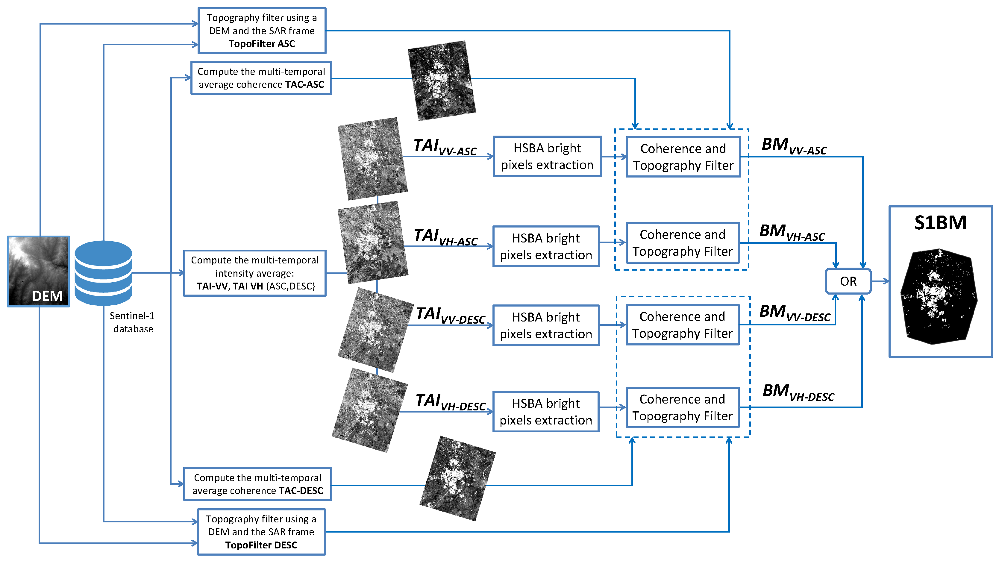
The selected areas focus on test sites located in semiarid and arid regions in the Mediterranean region and Northern Africa. The five sites are located respectively in Portugal, Turkey, Israel, Egypt, and Tunisia, as shown in Figure 2. The test sites were selected in the framework of the Urban Round-Robin exercise, supported by the European Space Agency (ESA), as it is well known that both optical and SAR data face major issues for urban area mapping in semiarid and arid regions [53]. The selection of these areas also aimed to reduce land cover uncertainties precisely in arid areas. Indeed, in the framework of the Climate Change Initiative (CCI), it has been stated that the uncertainty in the balance between grass and bare soil fraction in arid parts of Africa, central Asia, and central Australia is influencing albedo and evapotranspiration in all models, directly impacting uncertainties in global carbon, hydrology, and energy budgets [54].
The dataset consists of a multi-temporal series of Sentinel-1 IW images acquired on a monthly basis over the whole of 2016. For each test site, two time series comprising 12 VV- and 12 VH-polarization S-1 images acquired from both ascending and descending orbits were employed. The preprocessing steps include image calibration, terrain geocoding, topographic normalization, and multi-temporal averaging. For all five test sites, the input intensities were log-transformed and no further filtering nor resampling was applied. The images were processed at their original resolution in order to guarantee the same spatial resolution, i.e., 20 m, for the resulting building maps. The coherence was computed for each successive pair of images in the dataset (11 coherence images), first by generating an interferogram and then by estimating the coherence with a sliding window of 5 × 5 pixels. Both the intensity and coherence images of each set are stacked and the temporal average of intensity and coherence for both ASC&DESC and VV&VH are computed. The resulting datasets, defined as , and , are used as inputs for the proposed method.
4. Results
In this section, we present the results of the proposed algorithm for the five regions introduced in Section 3 and evaluate them by comparing the generated maps with the GUF product. The latter is a global-scale product that is derived from the information provided by a SAR sensor, albeit with a different spatial resolution and wavelength (X-band). The choice of GUF was made for the following reasons: it has a similar spatial resolution (i.e., 12.5 m), it is available at a global scale, and it is based on SAR data. This similarity in product characteristics allows a comparison to be performed that is both extensive and consistent. However, it goes without saying that the GUF cannot be considered a ’ground truth’, since it is derived from SAR data and, as a result, suffers from inherent classification uncertainty. Therefore, in the following, we intend to use the GUF for a cross-comparison in order to assess the agreement of S1BM with the established GUF product. This allows the capabilities of S-1 to be characterized to provide building maps on the global scale. In order to perform a pixel-by-pixel comparison between the two products, the GUF was resampled to 20 m, as were S1BM maps.
Figure 3 shows examples of the cross-comparison between the GUF and S1BM for the five selected test cases. The general agreement between the two products is evident, although differences are present and confirmed by the values reported in the confusion matrices (see Table 1). Table 1 reports the quantitative assessment of the entire areas through the overall accuracy (OA) and the K-coefficient indices together with the confusion matrices [55].
, the percentage of pixels that present an agreement between both maps with respect to the total number of classified pixels, is expressed as follows:
where is the number of pixels classified as buildings by S1BM and the GUF, is the number of pixels classified as not being buildings by S1BM and the GUF, and N is the total number of classified pixels.
The K-coefficient is defined as
where is the number pixels classified as buildings by S1BM, is the number pixels classified as buildings by GUF, is the number of pixels classified as not being buildings by S1BM, and is the number pixels classified as not being buildings by GUF.
It is important to highlight that the test cases are composed of millions of pixels (between 52 and 169 million for Egypt and Portugal, respectively), which allows for a meaningful statistical comparison. The overall accuracy ranges between 92% and 98%, thereby emphasizing the good agreement between the classifications obtained with the two algorithms. The K-coefficient reaches values exceeding 0.4 in four test areas (Turkey, Egypt, Portugal, and Israel), for which we can ascertain that there is a fairly good agreement between the two maps, while it equals 0.29 for the Tunisian test case, for which the agreement is thus rather poor.
5. Discussion
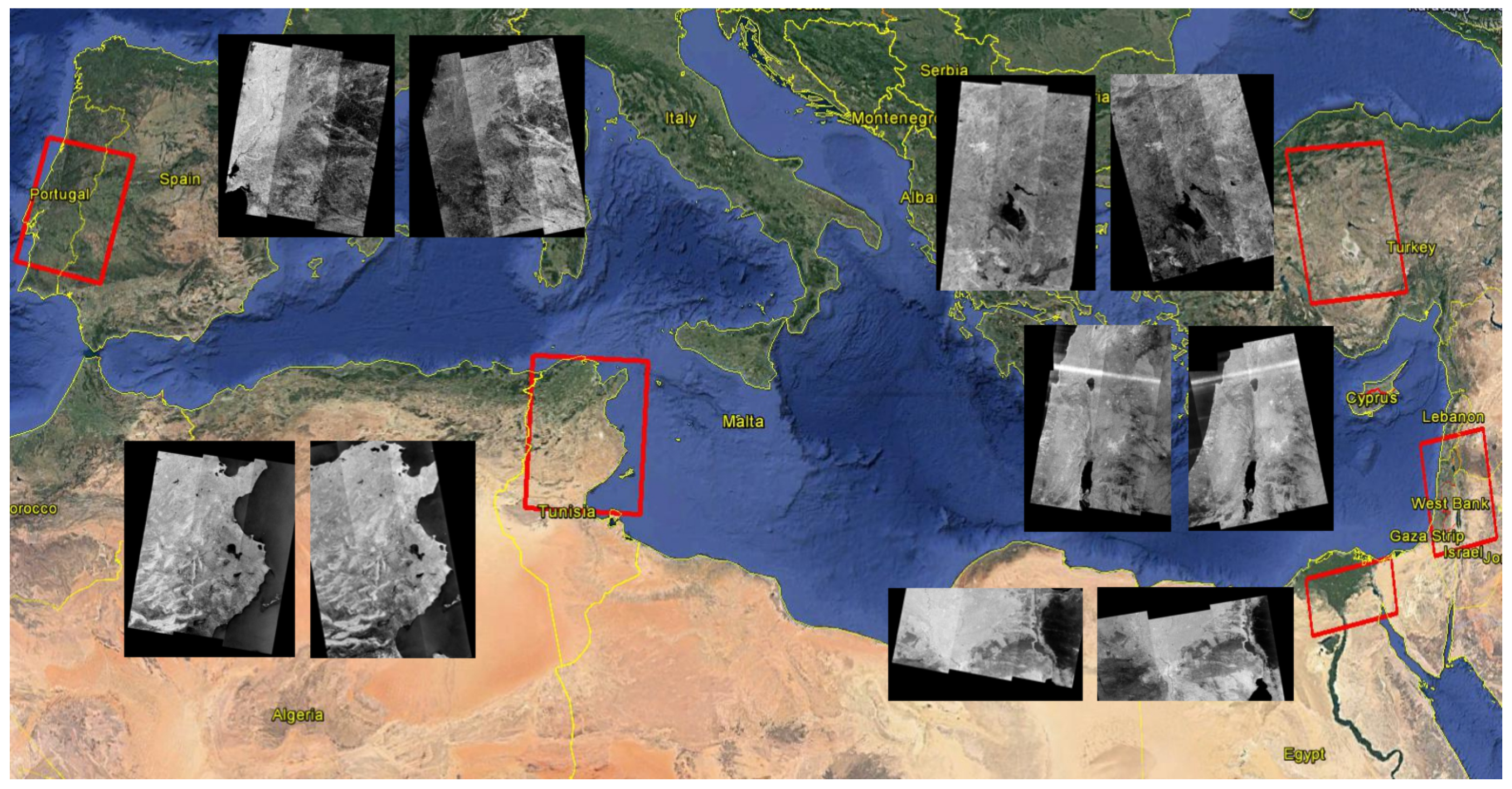
Looking at the confusion matrices, it is obvious that, overall, the proposed approach tends to underestimate building areas with respect to the GUF. There are three main reasons for this result: (i) the difference in the spatial resolution of source data (i.e., 20 m for Sentinel-1 vs. 3 m for TerraSAR-X), (ii) the difference in features used to delineate buildings (i.e., texture-based method for the GUF vs. pixel-based method for S1BM), and (iii) the difference in the semantic meaning of the two products (GUF and S1BM). For the first reason, it is worth indicating that, although the resolution of the GUF product is 12.5 m and thus rather close to the 20 m of S1BM, the 3 m spatial resolution of its source data is actually much higher. Therefore, due to the S-1 sensor resolution being limited to 20 m, small-sized buildings that are detectable at a 3 m resolution may be undetectable with S-1 data. Regarding the features used for extracting building areas, the GUF adopts speckle divergence, which is a textural parameter calculated using a kernel of a predefined size. This process implies a decrease in the resolution of the image. While the approach is very efficient for attenuating the speckle effect, it tends to include in the building class the area that is in the immediate vicinity of the actual building. Contrary to the GUF, the approach presented here focuses on identifying pixels characterized by high backscattering values that represent the double-bounce effect. In our study, it was possible to adopt a pixel-based approach because the speckle effect is attenuated by computing the multi-temporal average. The availability of large collections of S-1 images is thus a prerequisite for applying the method presented here. In this context, it is worth mentioning that the InSAR coherence feature, while extracted with a square kernel of a certain size, is used to remove false alarms from the final building map without decreasing its spatial resolution. There is also a semantic difference between the two products. S1BM is based on the detection of the DB feature, which is considered representative of the presence of a building. The GUF, on the other hand, starts from the detected DB to delineate urban settlements that may also include, for example, streets and parking lots. Moreover, some mismatches may occur due to the differences in the acquisition time of the images used. The TerraSAR-X dataset for extracting the GUF was acquired between 2011 and 2013, while the S-1 dataset was acquired in 2016. An example of this is shown in Figure 4, where it is possible to identify new settlements in the S1BM with respect to the GUF. We can see the new buildings in the corresponding area by visually comparing the optical images acquired in 2013 and 2016 (Figure 4c,d). For all these reasons, it can be expected that the difference in the number of pixels labeled, respectively, as “urban footprint” and “buildings” is due to the intrinsic difference between the characteristics of the two products. However, in spite of this, the overall accuracies indicate a rather good agreement between the two maps. It is also worth pointing out that to obtain the GUF product, 3 years of TerraSAR-X acquisitions (2011–2013) were necessary, while, to generate the S1BM at the global scale, 1 year, as is the case with this work, or less may be sufficient.
Most of the observed overdetection is related to the foreshortening effect in mountainous areas where the low resolution of the available DEM prevents the extraction of accurate LIA maps that would potentially allow the effect to be mitigated. The problem is most apparent in arid areas, where rocks are practically bare and the temporal coherence is high and constant. In such circumstances, not even the consideration of InSAR coherence allows the corresponding false alarms to be reduced. We observe this type of overdetection effect mostly in the Israel and Tunisia test cases, as can be seen in the examples shown in Figure 3. In the Israel dataset, some areas might be affected by the radio frequency interference (RFI) [56], as shown in Figure 2 (bright continuous stripes, in the northern part of the images, aligned with the range direction and present in both ascending and descending orbits), which causes some additional overdetection. Moreover, it is worth noting that the S1BM is obtained using only S-1 data and the SRTM DEM. Since the objective of our study is to show the potential of S-1 for generating building maps, no other images were used. This is not the case for the GUF, which removes some false alarms using other existing land cover layers during post-processing.
To highlight the individual benefits of the different features included in the processing chain, we calculated the K-coefficient and the overall accuracies for the five test cases using different combinations of inputs. The results are reported in Table 2. The analysis of these results shows that the role of the coherence and the LIA is to significantly improve the accuracy of the classification where only the intensity is considered. The InSAR coherence derived from S1 takes advantage of the sensor’s acquisition characteristics, being extracted in a consistent and systematic way, which allows an accurate classification of built-up areas. Most importantly, the use of the full set of features provides the highest accuracy for three test cases, while in the other two, which use only the VH channel, coherence and LIA yield better performances. Although in two cases the highest accuracies are obtained with a reduced dataset, the results are still rather close to those obtained with the full dataset. We would therefore argue that for generating a global product that is both reliable and accurate, it is preferable to make use of the full dataset.
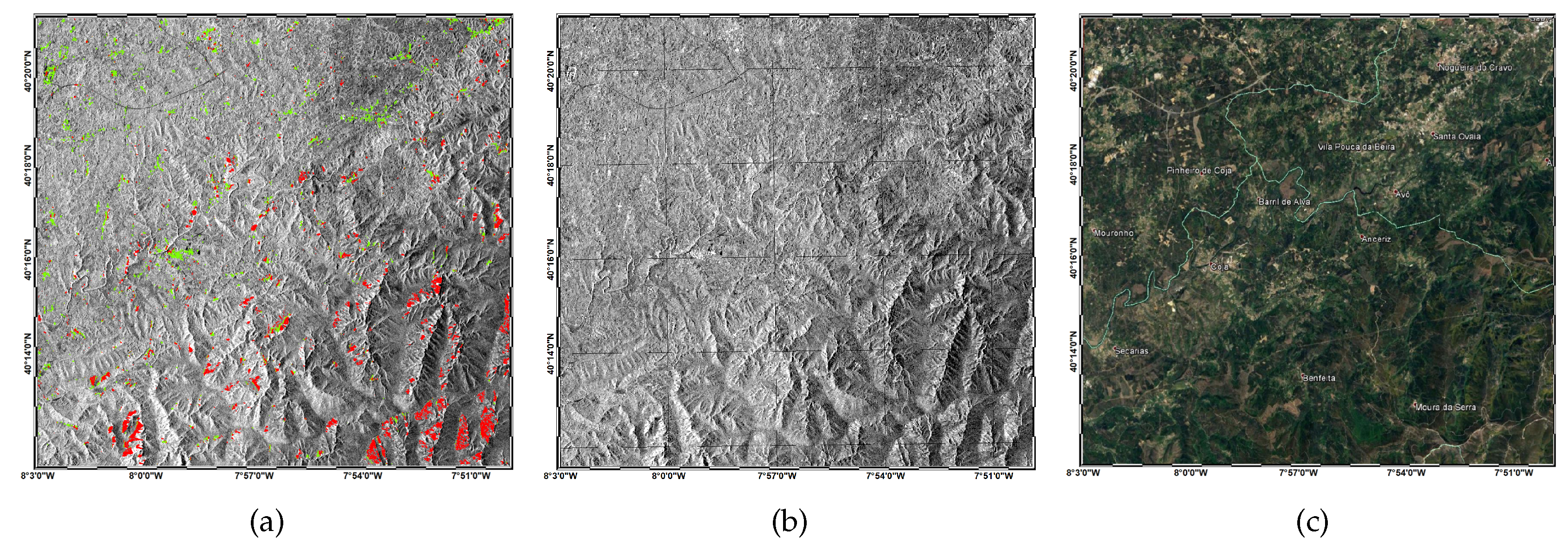
Examples of the role of the coherence and the LIA are shown in Figure 5 and Figure 6, respectively, where red pixels highlight the overdetected areas, and green pixels identify the buildings after the removal of false alarms due to vegetation and foreshortening in mountainous areas. In these two figures, the role of these two features in the classification results is then evidenced.
Although the results show that S-1 can provide essential information for generating land cover maps and, in particular, for delineating built-up areas, further work and efforts are required to cope with the remaining false alarms. For instance, especially in mountainous areas, the accuracy of the S1BM is affected by the resolution of the DEM. Other data sources, such as the one provided by the Sentinel-2 mission, could be exploited to remove some of the false alarms. Moreover, a higher-resolution and higher-precision DEM could be helpful to provide a more accurate LIA that would allow the removal of the foreshortening caused by steep slopes. Another important aspect worth investigating is the possibility to reduce the number of images employed, as this would allow the speeding-up of the whole process. Such developments would be especially useful when envisaging the generation of a global product and for regularly and frequently updating the resulting maps.
6. Conclusions
In this paper, we carried out an experiment to assess the capability of S-1 to map buildings by making use of IW images with a resolution of 20 m. In particular, the newly developed algorithm exploits the dual-polarization capability of S-1 (i.e., VV/VH in our case) and takes advantage of the particular characteristics of this satellite mission, such as the systematic imaging of the Earth, high revisit time, and small orbital tube. All these characteristics are particularly important when making use of InSAR coherence for classification purposes. As demonstrated in this study, the multi-temporal InSAR coherence, as a consistent and systematic feature, allows for a better characterization of urban areas. Moreover, the systematic S-1 acquisition plan allows us to frequently update buildings maps at a large scale, more than once per year. The algorithm was developed in the framework of the Urban Round-Robin exercise, supported by the European Space Agency (ESA) through the ESA Land Cover Climate Change Initiative (CCI), which aimed to evaluate the capability of S-1 to map urban areas. In this context, GCOS [1] expressed the need for annually updated urban maps with a resolution of 10–30 m and the detection of the land cover change derived therefrom. The S-1 dataset was made available through the Urban Round-Robin exercise, encompassing five different test sites located in challenging semiarid and arid regions in the Mediterranean region and Northern Africa.
For the five areas tested, the comparison with the GUF product from TerraSAR-X data showed an overall accuracy agreement between the two products in the range between 92% and 98%. The corresponding K-coefficient presents values of about 0.4, which shows the differences between the two products in terms of the spatial resolution and feature types employed. Although the test cases have different typologies of urban areas and vegetation, the algorithm provides similar results, thereby highlighting the potential for generalizing and upscaling. Furthermore, the results provide evidence that the two hypotheses that drive the setup of the algorithm, i.e., very high backscattering and time coherence for the buildings in the SAR images, are indeed valid and can be exploited to produce global building maps using S-1 images with a resolution of 20 m. This generalization has also been possible thanks to the adaptive thresholding approach used to identify very bright pixels in both VV and VH channels. The approach automatically and accurately parameterizes the distribution function of the class of interest by identifying tiles of variable size where the target class and its background are well balanced in terms of number of pixels. The systematic use of the InSAR temporal coherence to remove pixels that show high backscattering and low InSAR coherence from the classification, e.g., certain types of vegetation, was possible thanks to the small orbital S-1 tube. This prevents the drop-off of coherence due to high perpendicular baselines, which are known to be most relevant in urban areas.
Author Contributions
Conceptualization, M.C.; Formal analysis, M.C. and R.P.; Investigation, M.C. and R.P.; Methodology, M.C.; Software, M.C., R.P., R.H. and P.M.; Validation, R.P.; Writing—original draft, M.C. and R.P.; Writing—review & editing, M.C., R.P., R.H., P.M. And C.L.-M.
Funding
This research was funded by the National Research Fund of Luxembourg (FNR) through the MOSQUITO project, grant number C15/SR/10380137.
Acknowledgments
The authors would like to thank the European Space Agency (ESA) Climate Change Initiative (CCI) Land Cover (LC) project for making the dataset available and the German Aerospace Center (DLR) for providing us with the GUF data for our areas of interest.
Conflicts of Interest
The authors declare no conflict of interest.
References
- GCOS. The Global Observing System for Climate: Implementation Needs. Technical Report, 2016. Available online: https://unfccc.int/sites/default/files/gcos_ip_10oct2016.pdf (accessed on 16 November 2018).
- Gong, P.; Wang, J.; Yu, L.; Zhao, Y.; Zhao, Y.; Liang, L.; Niu, Z.; Huang, X.; Fu, H.; Liu, S.; et al. Finer resolution observation and monitoring of global land cover: first mapping results with Landsat TM and ETM+ data. Int. J. Remote Sens. 2013, 34, 2607–2654. [Google Scholar] [CrossRef]
- Pitman, A.J.; de Noblet-Ducoudré, N.; Avila, F.B.; Alexander, L.V.; Boisier, J.P.; Brovkin, V.; Delire, C.; Cruz, F.; Donat, M.G.; Gayler, V.; et al. Effects of land cover change on temperature and rainfall extremes in multi-model ensemble simulations. Earth Syst. Dyn. 2012, 3. [Google Scholar] [CrossRef]
- Henderson, F.M.; Xia, Z.G. SAR Applications in Human Settlement Detection, Population Estimation and Urban Land Use Pattern Analysis: A Status Report. IEEE Trans. Geosci. Remote Sens. 1997, 35, 79–85. [Google Scholar] [CrossRef]
- United Nations. World Urbanization Prospects—The 2014 Revision. Technical Report, 2014. Available online: http://esa.un.org/unpd/wup/ (accessed on 25 October 2018).
- ESA. The Land Cover Climate Change Initiative (CCI). Technical Report, European Space Agency, 2010. Available online: http://www.esa-landcover-cci.org/ (accessed on 25 October 2018).
- Schneider, A.; Friedl, M.A.; Potere, D. Mapping global urban areas using MODIS 500-m data: New methods and datasets based on urban ecoregions. Remote Sens. Environ. 2010, 114, 1733–1746. [Google Scholar] [CrossRef]
- Pesaresi, M.; Ehrlich, D.; Caravaggi, I.; Kauffmann, M.; Louvrier, C. Toward Global Automatic Built-Up Area Recognition Using Optical VHR Imagery. IEEE J. Sel. Top. Appl. Earth Obs. Remote Sens. 2011, 4, 923–934. [Google Scholar] [CrossRef]
- Pesaresi, M.; Huadong, G.; Blaes, X.; Ehrlich, D.; Ferri, S.; Gueguen, L.; Halkia, M.; Kauffmann, M.; Kemper, T.; Lu, L.; et al. A Global Human Settlement Layer From Optical HR/VHR RS Data: Concept and First Results. IEEE J. Sel. Top. Appl. Earth Obs. Remote Sens. 2013, 6, 2102–2131. [Google Scholar] [CrossRef]
- Benedek, C.; Descombes, X.; Zerubia, J. Building Development Monitoring in Multitemporal Remotely Sensed Image Pairs with Stochastic Birth-Death Dynamics. IEEE Trans. Pattern Anal. Mach. Intell. 2012, 34, 33–50. [Google Scholar] [CrossRef] [PubMed] [Green Version]
- Grinias, I.; Panagiotakis, C.; Tziritas, G. MRF-based Segmentation and Unsupervised Classification for Building and Road Detection in Peri-urban Areas of High-resolution. ISPRS J. Photogramm. Remote Sens. 2016, 122, 145–166. [Google Scholar] [CrossRef]
- Chini, M.; Chiancone, A.; Stramondo, S. Scale Object Selection (SOS) through a hierarchical segmentation by a multi-spectral per-pixel classification. Pattern Recognit. Lett. 2014, 49, 214–223. [Google Scholar] [CrossRef] [Green Version]
- Dekker, R.J. Texture Analysis and Classification of ERS SAR Images for Map Updating of Urban Areas in The Netherlands. IEEE Trans. Geosci. Remote Sens. 2003, 41. [Google Scholar] [CrossRef]
- Dell’Acqua, F.; Gamba, P. Texture-based characterization of urban environments on satellite SAR images. IEEE Trans. Geosci. Remote Sens. 2003, 41, 153–159. [Google Scholar] [CrossRef]
- Dell’Acqua, F.; Gamba, P. Discriminating urban environments using multiscale texture and multiple SAR images. Int. J. Remote Sens. 2006, 27, 3797–3812. [Google Scholar] [CrossRef]
- Voisin, A.; Krylov, V.A.; Moser, G.; Serpico, S.B.; Zerubia, J. Classification of Very High Resolution SAR Images of Urban Areas Using Copulas and Texture in a Hierarchical Markov Random Field Model. IEEE Geosci. Remote Sens. Lett. 2013, 10. [Google Scholar] [CrossRef]
- Baselice, F.; Ferraioli, G. Statistical Edge Detection in Urban Areas Exploiting SAR Complex Data. IEEE Geosci. Remote Sens. Lett. 2012, 9, 185–189. [Google Scholar] [CrossRef]
- Matikainen, L.; Hyyppä, J.; Engdahl, M.E. Mapping Built-up Areas from Multitemporal Interferometric SAR Images—A Segment-based Approach. Photogramm. Eng. Remote Sens. 2006, 6, 701–714. [Google Scholar] [CrossRef]
- Corbane, C.; Lemoine, G.; Pesaresi, M.; Kemper, T.; Sabo, F.; Ferri, S.; Syrris, V. Enhanced automatic detection of human settlements using Sentinel-1 interferometric coherence. Int. J. Remote Sens. 2017, 39, 842–853. [Google Scholar] [CrossRef]
- Xiang, D.; Tang, T.; Ban, Y.; Su, Y.; Kuang, G. Unsupervised polarimetric SAR urban area classification based on model-based decomposition with cross scattering. ISPRS J. Photogramm. Remote Sens. 2016, 1116, 86–100. [Google Scholar] [CrossRef]
- Stasolla, M.; Gamba, P. Spatial Indexes for the Extraction of Formal and Informal Human Settlements From High-Resolution SAR Images. IEEE J. Sel. Top. Appl. Earth Obs. Remote Sens. 2008, 1. [Google Scholar] [CrossRef]
- Gamba, P.; Lisini, G. Fast and Efficient Urban Extent Extraction Using ASAR Wide Swath Mode Data. IEEE J. Sel. Top. Appl. Earth Obs. Remote Sens. 2013, 6. [Google Scholar] [CrossRef]
- Lisini, G.; Salentinig, A.; Du, P.; Gamba, P. SAR-Based Urban Extents Extraction: From ENVISAT to Sentinel-1. IEEE J. Sel. Top. Appl. Earth Obs. Remote Sens. 2017. [Google Scholar] [CrossRef]
- Ban, Y.; Jacob, A.; Gamba, P. Spaceborne SAR data for global urban mapping at 30 m resolution using a robust urban extractor. ISPRS J. Photogramm. Remote Sens. 2015, 103. [Google Scholar] [CrossRef]
- Gamba, P.; Aldrighi, M.; Stasolla, M. Robust Extraction of Urban Area Extents in HR and VHR SAR Images. IEEE J. Sel. Top. Appl. Earth Obs. Remote Sens. 2011, 4. [Google Scholar] [CrossRef]
- Esch, T.; Heldens, W.; Hirner, A.; Keil, M.; Marconcini, M.; Roth, A.; Zeidler, J.; Dech, S.; Strano, E. Breaking new ground in mapping human settlements from space – The Global Urban Footprint. ISPRS J. Photogramm. Remote Sens. 2017, 134. [Google Scholar] [CrossRef]
- Chini, M.; Hostache, R.; Giustarinij, L.; Matgen, P. A Hierarchical Split-Based Approach (HSBA) for automatically mapping changes using SAR images of variable size and resolution: flood inundation as a test case. IEEE Trans. Geosci. Remote Sens. 2017, 55, 6975–6988. [Google Scholar] [CrossRef]
- Giustarini, L.; Hostache, R.; Kavetski, D.; Chini, M.; Corato, G.; Schlaffer, S.; Matgen, P. Probabilistic Flood Mapping Using Synthetic Aperture Radar Data. IEEE Trans. Geosci. Remote Sens. 2016, 54, 6958–6969. [Google Scholar] [CrossRef]
- Giustarini, L.; Hostache, R.; Matgen, P.; Schumann, G.J.P.; Bates, P.D.; Mason, D.C. A Change Detection Approach to Flood Mapping in Urban Areas Using TerraSAR-X. IEEE Trans. Geosci. Remote Sens. 2013, 51, 2417–2430. [Google Scholar] [CrossRef]
- Franceschetti, G.; Iodice, A.; Riccio, D. A canonical problem in electromagnetic backscattering from buildings. IEEE Trans. Geosci. Remote Sens. 2002, 40. [Google Scholar] [CrossRef]
- Ferro, A.; Brunner, D.; Bruzzone, L.; Lemoine, G. On the relationship between double bounce and the orientation of buildings in VHR SAR images. IEEE Geosci. Remote Sens. Lett. 2011, 8. [Google Scholar] [CrossRef]
- Pulvirenti, L.; Chini, M.; Pierdicca, N.; Boni, G. Use of SAR Data for Detecting Floodwater in Urban and Agricultural Areas: The Role of the Interferometric Coherence. IEEE Trans. Geosci. Remote Sens. 2016, 54. [Google Scholar] [CrossRef]
- Brunner, D.; Lemoine, G.; Bruzzone, L. Earthquake damage assessment of buildings using VHR optical and SAR imagery. IEEE Trans. Geosci. Remote Sens. 2010, 48, 2403–2420. [Google Scholar] [CrossRef]
- Chini, M. Building Damage from Multi-resolution, Object-Based, Classification Techniques. In Encyclopedia of Earthquake Engineering; Beer, M., Kougioumtzoglou, I.A., Patelli, E., Au, I.S.K., Eds.; Springer: Berlin/Heidelberg, Germany, 2014; pp. 1–11. [Google Scholar]
- Sato, A.; Yamaguchi, Y.; Singh, G.; Park, S.E. Four-Component Scattering Power Decomposition with Extended Volume Scattering Model. IEEE Geosci. Remote Sens. Lett. 2011, 9. [Google Scholar] [CrossRef]
- Thiele, A.; Cadario, E.; Schulz, K.; Thönnessen, U.; Soerge, U. Building recognition from multi-aspect high-resolution InSAR data in urban areas. IEEE Trans. Geosci. Remote Sens. 2007, 45, 3583–3593. [Google Scholar] [CrossRef]
- Zebker, H.; Villasenor, J. Decorrelation in interferometric radar echoes. IEEE Trans. Geosci. Remote Sens. 1992, 30. [Google Scholar] [CrossRef]
- Chini, M.; Albano, M.; Saroli, M.; Pulvirenti, L.; Moro, M.; Bignami, C.; Falcucci, E.; Gori, S.; Modoni, G.; Pierdicca, N.; et al. Coseismic liquefaction phenomenon analysis by COSMO-SkyMed: 2012 Emilia (Italy) earthquake. Int. J. Appl. Earth Obs. Geoinf. 2015, 39. [Google Scholar] [CrossRef]
- Kropatsch, W.G.; Strobl, D. The generation of SAR layover and shadow maps from digital elevation models. IEEE Trans. Geosci. Remote Sens. 1990, 28, 98–107. [Google Scholar] [CrossRef]
- Farr, T.G. The Shuttle Radar Topography Mission. Rev. Geophys. 2007. [Google Scholar] [CrossRef]
- Esch, T.; Thiel, M.; Schenk, A.; Roth, A.; Müller, A.; Dech, S. Delineation of Urban Footprints From TerraSAR-X Data by Analyzing Speckle Characteristics and Intensity Information. IEEE Trans. Geosci. Remote Sens. 2010, 48. [Google Scholar] [CrossRef]
- Esch, T.; Schenk, A.; Ullmann, T.; Thiel, M.; Roth, A.; Dech, S. Characterization of Land Cover Types in TerraSAR-X Images by Combined Analysis of Speckle Statistics and Intensity Information. IEEE Trans. Geosci. Remote Sens. 2011, 49, 1911–1925. [Google Scholar] [CrossRef]
- Esch, T.; Marconcini, M.; Felbier, A.; Roth, A.; Heldens, W.; Huber, M.; Schwinger, M.; Taubenböck, H.; Müller, A.; Dech, S. Urban Footprint Processor—Fully Automated Processing Chain Generating Settlement Masks From Global Data of the TanDEM-X Mission. IEEE Geosci. Remote Sens. Lett. 2013, 10. [Google Scholar] [CrossRef] [Green Version]
- Pierdicca, N.; Pulvirenti, L.; Boni, G.; Squicciarino, G.; Chini, M. Mapping Flooded Vegetation Using COSMO-SkyMed: Comparison With Polarimetric and Optical Data Over Rice Fields. IEEE J. Sel. Top. Appl. Earth Obs. Remote Sens. 2017, 10, 2650–2662. [Google Scholar] [CrossRef]
- Richards, J.A. Remote Sensing With Imaging Radar; Springer: Berlin/Heidelberg, Germany, 2009. [Google Scholar]
- Foody, G.M.; Mathur, A.; Sanchez-Hernande, C.; Boyd, D.S. Training set size requirements for the classification of a specific class. Remote Sens. Environ. 2006, 104. [Google Scholar] [CrossRef]
- Mack, B.; Roscher, R.; Waske, B. Can I Trust My One-Class Classification? Remote Sens. 2014, 6. [Google Scholar] [CrossRef]
- Mack, B.; Roscher, R.; Stenzel, S.; Feilhauer, H.; Schmidtlein, S.; Waske, B. Mapping raised bogs with an iterative one-class classification approach. ISPRS J. Photogramm. Remote Sens. 2016, 120. [Google Scholar] [CrossRef]
- Xie, H.; Pierce, L.E.; Ulaby, F.T. Statistical Properties of Logarithmically Transformed Speckle. IEEE Trans. Geosci. Remote Sens. 2002, 40, 721–727. [Google Scholar] [CrossRef]
- Marquardt, D.W. An algorithm for least-squares estimation of nonlinear parameters. J. Soc. Ind. Appl. Math. 1963, 11. [Google Scholar] [CrossRef]
- Ashman, K.M.; Bird, C.M.; Zepf, S.E. Detecting bimodality in astronomical datasets. Astrophysics 1994, 108, 2348–2361. [Google Scholar] [CrossRef]
- Haralick, R.M.; Shapiro, L.G. Image segmentation techniques. Comput. Vis. Graph. Image Process. 1985, 29, 100–132. [Google Scholar] [CrossRef]
- ESA CCI. Land Cover Newsletter, Special Issue. Technical Report, October 2015. Available online: https://www.esa-landcover-cci.org/?q=webfm_send/86 (accessed on 25 October 2018).
- ESA CCI. Uncertainty in Plant Functional Type Distributions and Its Impact on Land Surface Models, Land Cover Newsletter, Issue 7. Technical Report, April 2017. Available online: https://www.esa-landcover-cci.org/?q=webfm_send/88 (accessed on 25 October 2018).
- Hudson, W.; Ramm, C. Correct formulation of the Kappa coefficient of agreement. Photogramm. Eng. Remote Sens. 1987, 53, 421–422. [Google Scholar]
- Li, Y.; Monti Guarnieri, A.; Hu, C.; Rocca, F. Performance and Requirements of GEO SAR Systems in the Presence of Radio Frequency Interferences. Remote Sens. 2018, 10, 82. [Google Scholar] [CrossRef]
Figure 1.
Block diagram of the algorithm that performs the building extraction from multi-temporal synthetic aperture radar (SAR) intensity and InSAR coherence stacks extracted from Sentinel-1 data.
Figure 1.
Block diagram of the algorithm that performs the building extraction from multi-temporal synthetic aperture radar (SAR) intensity and InSAR coherence stacks extracted from Sentinel-1 data.

Figure 2.
Locations of the five test sites.

Figure 3.
Sentinel-1 (S-1) Buildings Map (S1BM) versus the Global Urban Footprint (GUF) for the Egypt (a,b), Israel (c,d), Portugal (e,f), Tunisia (g,h), and Turkey (i,j) test cases. Left column: confusion maps (Red: buildings detected only by S1BM, Green: overlap of detected buildings by S1BM & GUF, blue: buildings detected only by GUF, background: S1 backscattering intensity). Right column: examples of S1 VV intensity datasets.


Figure 4.
Illustration of new built-up areas identified in S1BM: (a) red—buildings detected only by S1BM; green—overlap of detected buildings by S1BM and the GUF; blue—buildings detected only by GUF. (b) Corresponding S1 image. Optical images from (c) 2013 and (d) 2016 (source: Google Earth).
Figure 4.
Illustration of new built-up areas identified in S1BM: (a) red—buildings detected only by S1BM; green—overlap of detected buildings by S1BM and the GUF; blue—buildings detected only by GUF. (b) Corresponding S1 image. Optical images from (c) 2013 and (d) 2016 (source: Google Earth).

Figure 5.
Illustration of the usefulness of the coherence information for reducing the vegetation false alarms which are strongly noticeable in the intensity TAI (temporal average intensity) image, Egypt (c). (a) red—areas removed by the coherence (temporal average coherence (TAC)) filter, green—areas retained by the TAC filter in the S1BM product; (b) optical image of the scene (source: Google Earth); (c) intensity image; (d) coherence image.

Figure 6.
Illustration of the removal of foreshortening regions with building-like backscattering values, Portugal. (a) Red—areas removed by the topography filter, green—areas retained by the topography filter in the S1BM product; (b) intensity image; (c) optical image of the scene (source: Google Earth).


Table 1.
Quantitative analysis and confusion matrices for the five different test cases. S1BM & GUF cross-comparison.
Table 1.
Quantitative analysis and confusion matrices for the five different test cases. S1BM & GUF cross-comparison.
| OA K-Coefficient | GUF | ||||
|---|---|---|---|---|---|
| Building | Non-Building | Total | S1BM | ||
| Egypt | 94.49% 0.40 | 1,098,252 1,958,899 3,057,151 | 922,663 48,389,217 49,311,880 | 2,020,915 50,348,116 52,369,031 | Building Non-Building Total |
| Israel | 91.55% 0.41 | 3,243,643 3,171,558 6,415,201 | 4,441,721 79,280,291 83,722,012 | 7,685,364 82,451,849 90,137,213 | Building Non-Building Total |
| Portugal | 97.93% 0.47 | 1,615,984 1,937,363 3,553,347 | 1,544,888 163,726,890 165,271,778 | 3,160,872 165,664,253 168,825,125 | Building Non-Building Total |
| Tunisia | 95.60% 0.29 | 140,9270 672,887 2,082,157 | 5,525,183 133,535,295 139,060,478 | 6,934,453 134,208,182 141,142,635 | Building Non-Building Total |
| Turkey | 96.94% 0.45 | 1,108,717 484,987 1,593,704 | 2,035,978 78,972,860 81,008,838 | 3,144,695 79,457,847 82,602,542 | Building Non-Building Total |
Table 2.
Quantitative analysis for different combinations of the inputs and filters. CC—InSAR coherence filter, LIA—local incidence angle filter (best performances are highlighted in bold font).
Table 2.
Quantitative analysis for different combinations of the inputs and filters. CC—InSAR coherence filter, LIA—local incidence angle filter (best performances are highlighted in bold font).
| S1BM & GUF Cross-Comparison: Overall Accuracy, K-Coefficient | ||||||
|---|---|---|---|---|---|---|
| VV-ASC&DESC VH-ASC&DESC CC, LIA | VV-ASC&DESC VH-ASC&DESC | VV-ASC CC, LIA | VV-DESC CC, LIA | VH-ASC CC, LIA | VH-DESC CC, LIA | |
| Egypt | 94% 0.40 | 93% 0.36 | 94% 0.24 | 94% 0.26 | 94% 0.25 | - |
| Israel | 91% 0.41 | 65% 0.16 | 92% 0.32 | 92% 0.29 | 91% 0.31 | 91% 0.29 |
| Portugal | 98% 0.47 | 83% 0.12 | 98% 0.29 | 98% 0.42 | 98% 0.24 | 98% 0.33 |
| Tunisia | 96% 0.30 | 90% 0.16 | 98% 0.35 | 97% 0.14 | 98% 0.40 | 98% 0.28 |
| Turkey | 97% 0.45 | 90% 0.20 | 98% 0.40 | 97% 0.38 | 98% 0.48 | 98% 0.49 |
© 2018 by the authors. Licensee MDPI, Basel, Switzerland. This article is an open access article distributed under the terms and conditions of the Creative Commons Attribution (CC BY) license (http://creativecommons.org/licenses/by/4.0/).
Share and Cite
MDPI and ACS Style
Chini, M.; Pelich, R.; Hostache, R.; Matgen, P.; Lopez-Martinez, C. Towards a 20 m Global Building Map from Sentinel-1 SAR Data. Remote Sens. 2018, 10, 1833. https://0-doi-org.brum.beds.ac.uk/10.3390/rs10111833
AMA Style
Chini M, Pelich R, Hostache R, Matgen P, Lopez-Martinez C. Towards a 20 m Global Building Map from Sentinel-1 SAR Data. Remote Sensing. 2018; 10(11):1833. https://0-doi-org.brum.beds.ac.uk/10.3390/rs10111833
Chicago/Turabian StyleChini, Marco, Ramona Pelich, Renaud Hostache, Patrick Matgen, and Carlos Lopez-Martinez. 2018. "Towards a 20 m Global Building Map from Sentinel-1 SAR Data" Remote Sensing 10, no. 11: 1833. https://0-doi-org.brum.beds.ac.uk/10.3390/rs10111833
Note that from the first issue of 2016, this journal uses article numbers instead of page numbers. See further details here.