Article

Capability of Remotely Sensed Drought Indices for Representing the Spatio–Temporal Variations of the Meteorological Droughts in the Yellow River Basin

1
School of Water Conservancy and Environment, Zhengzhou University, Zhengzhou 450001, China
2
China Institute of Water Resources and Hydropower Research, the State Key Laboratory of Simulation and Regulation of Water Cycle in River Basin, Beijing 100038, China
3
School of Engineering, Newcastle University, Newcastle upon Tyne NE1 7RU, UK
*
Authors to whom correspondence should be addressed.
Remote Sens. 2018, 10(11), 1834; https://0-doi-org.brum.beds.ac.uk/10.3390/rs10111834
Submission received: 22 October 2018 / Revised: 17 November 2018 / Accepted: 18 November 2018 / Published: 20 November 2018
(This article belongs to the Section Remote Sensing in Agriculture and Vegetation)

Abstract

:
Due to the advantages of wide coverage and continuity, remotely sensed data are widely used for large-scale drought monitoring to compensate for the deficiency and discontinuity of meteorological data. However, few studies have focused on the capability of various remotely sensed drought indices (RSDIs) to represent the spatio–temporal variations of meteorological droughts. In this study, five RSDIs, namely the Vegetation Condition Index (VCI), Temperature Condition Index (TCI), Vegetation Health Index (VHI), Modified Temperature Vegetation Dryness Index (MTVDI), and Normalized Vegetation Supply Water Index (NVSWI), were calculated using monthly Normalized Difference Vegetation Index (NDVI) and land surface temperature (LST) from the Moderate Resolution Imaging Spectroradiometer (MODIS). The monthly NDVI and LST data were filtered by the Savitzky–Golay (S-G) filtering method. A meteorological station-based drought index represented by the Standardized Precipitation Evapotranspiration Index (SPEI) was compared with the RSDIs. Additionally, the dimensionless Skill Score (SS) method was adopted to identify the spatiotemporally optimal RSDIs for presenting meteorological droughts in the Yellow River basin (YRB) from 2000 to 2015. The results indicated that: (1) RSDIs revealed a decreasing drought trend in the overall YRB consistent with the SPEI except for in winter, and different variations of seasonal trends spatially; (2) the optimal RSDIs in spring, summer, autumn, and winter were VHI, TCI, MTVDI, and VCI, respectively, and the average correlation coefficient between the RSDIs and the SPEI was 0.577 (α = 0.05); and (3) different RSDIs have time lags of zero–three months compared with the meteorological drought index.

Graphical Abstract

1. Introduction

Drought is a complex and recurring natural disaster that occurs throughout the world and often has negative impacts on many sectors of society [1,2]. Droughts are increasing in frequency and severity, and their impact on human lives and the economy is accelerating due to growing levels of urbanization and an increasing number of extreme weather events [3,4,5]. The effective assessment of drought is an essential means towards achieving sustainable development. Traditional drought monitoring is based on data from meteorological stations. The relatively mature meteorological drought index includes the Palmer Drought Severity Index (PDSI) [6], the Standardized Precipitation Index (SPI) [7], and the Standardized Precipitation Evapotranspiration Index (SPEI) [8]. Despite the high accuracy of meteorological station data, the meteorological drought index is constrained by the insufficient spatial distribution of stations, and has difficulty in reflecting a wide range of drought information [9]. In 2015, 17 sustainable development goals (SDGs) were formally adopted at the UN Sustainable Development Summit, which clearly indicates that remote sensing technology has become an important way to reduce the risk of loss from drought disaster and achieve the goal of sustainable development [10,11]. Remote sensing technology makes up for the shortage of meteorological stations thanks to its advantages of objective, its timely, economic, and wide coverage, its continuous data, and its ability to extend traditional “point” measurements to information about the entire areas. Remote sensing has proved to be the most promising technology in drought monitoring, and is now widely used in drought prevention, response, recovery, and mitigation [12,13].
Many drought-monitoring methods based on remote sensing have been developed, including the vegetation index method, thermal inertia method, canopy temperature method, and microwave remote sensing method. As vegetation growth is closely related to soil moisture levels, the vegetation index method has become the main approach for monitoring agricultural drought based on remote sensing [14]. Kogan considered that the Vegetation Condition Index (VCI) is capable of monitoring drought and providing accurate drought information under different ecological environmental conditions in the United States. The VCI is suitable for monitoring the interannual dry–wet conditions and can eliminate the effects of climatic conditions, soil type, and topography, allowing comparison between different regions [15,16]. The Temperature Condition Index (TCI) is defined by the principle of elevated temperature and deficient water, and vegetation canopy or soil surface temperature increases with the rise of water stress. The TCI can reflect the adverse effects of high temperature on the growth of crops [17]. The Vegetation Health Index (VHI) is a health condition index that takes into account the effect of vegetation leaf surface and temperature on vegetation. The VHI is used to reflect the differences in the spatio–temporal patterns of drought and has a better effect of drought monitoring [18]. Sandholt et al. indicated that there was a triangular or trapezoidal relationship between the vegetation index and land surface temperature, and developed the Temperature Vegetation Dryness Index (TVDI) based on the scattered point feature space of these two parameters [19]. Wang et al. proposed the Modified Temperature Vegetation Dryness Index (MTVDI) based on the difference between one and the TVDI [20]. The MTVDI combines the special physiological and ecological significance of the vegetation index and land surface temperature; it is easy to understand and calculate, and is widely used in drought monitoring. Abbas et al. revised the Vegetation Supply Water Index (VSWI), and discovered that the physical mechanism of the Normalized Vegetation Supply Water Index (NVSWI) is much clearer [21]. The NVSWI is superior to the VSWI for the analysis of time series, it can express the actual drought situation, and has a prominent advantage in drought monitoring [22].
There are many remotely sensed drought indices (RSDIs), which use data from the Moderate Resolution Imaging Spectroradiometer (MODIS) for drought monitoring. While all of these RSDIs can be used to monitor drought, the capability of different indices varies with temporal and spatial patterns [23]. Klisch et al. quantified drought strength by calculating the VCI at the pixel level from de-noised MODIS Normalized Difference Vegetation Index (NDVI) data, and successfully applied drought products to drought monitoring in Kenya [24]. Zhang et al. used drought events during 2011 and 2012 to compare various RSDIs, and found that different RSDIs had differing characteristics and were suitable for specific environments [25]. The studies of Hao et al. and Du et al. indicated that studying the capability of RSDIs can better reveal drought characteristics, by comparing the drought monitoring ability of several different RSDIs [26,27]. RSDIs are used to quantitatively evaluate the effects of drought and directly determine the accuracy of drought monitoring; therefore, it is particularly important to study their capability under different spatio–temporal patterns. However, few studies have combined RSDIs with the meteorological drought index to assess whether the remotely sensed index is suitable for drought monitoring, and the research on the capability of RSDIs under different spatio–temporal patterns is insufficient [28,29]. Moreover, most of the methods to evaluate capability are based on a single statistical indicator (e.g., average deviation and root-mean-square error). While average deviation can reflect the overall deviation degree of remotely sensed and meteorological drought results in time-field or space-field, it cannot measure the similarity degree. Likewise, the correlation coefficient can measure the similarity degree between remotely sensed and meteorological drought, but it cannot reflect the actual deviation information. Due to the obvious temporal and spatial differences in drought, it is urgent to improve the comprehensiveness and objectivity of drought assessment through a composite statistical indicator with explicit significance. The latest development of Skill Score (SS) is a composite indicator that considers deviation and correlation coefficient synthetically [30,31]. By comparing the grade results of remotely sensed and meteorological drought, the spatio–temporal capability of RSDIs is quantitatively evaluated [32].
The capability of RSDIs should be fully considered on temporal and spatial scales. However, the systematic investigation of the spatio–temporal capability of RSDIs has not been carried out in the Yellow River basin (YRB). In view of this, the composite indicator SS was used for the first time in the YRB to quantitatively evaluate the capability of RSDIs in order to obtain the optimal RSDIs under different spatio–temporal patterns. We can elaborately and systematically reveal the highly precise RSDIs used to assess the YRB under different temporal and spatial patterns based on SS, so as to improve the accuracy of drought monitoring. The research results can provide a reasonable scientific assessment of the drought situation in the YRB and provide reference and basis for drought relief measures. It is of great practical significance to study the evolution and scientific development of drought under the changing environment in the YRB.

2. Materials and Methods
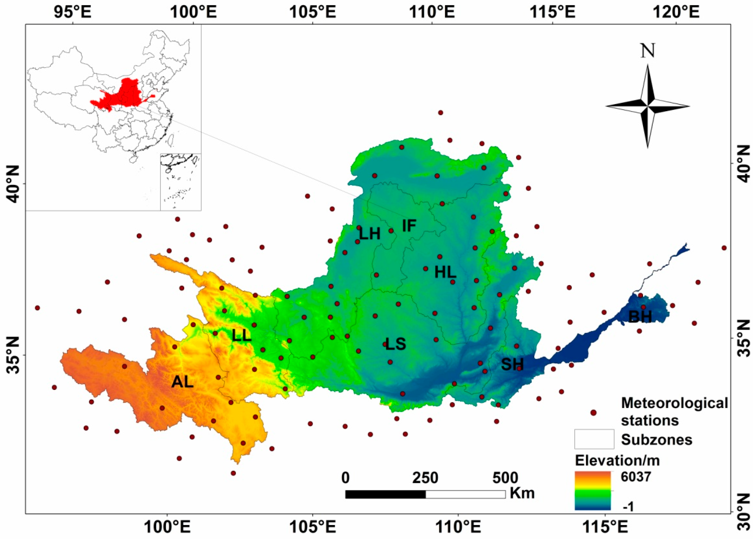
2.1. Study area

The Yellow River basin (YRB) is located between 95°53’–119°05’E and 32°10’–41°50’N. It originates in the Bayan Har Mountains and flows from Kenli County of Shandong Province to the Bohai Sea. Most of the YRB consists of arid and semi-arid areas with scarce water resources. Under the influence of climate change and human activities, the ecological environment of the YRB is fragile and has the basic characteristics of drought. The YRB is composed of eight water resource secondary subzones, namely, Above Longyangxia (AL), Longyangxia to Lanzhou (LL), Lanzhou to Hekou (LH), Inner Flow region (IF), Hekou to Longmen (HL), Longmen to Sanmenxia (LS), Sanmenxia to Huayuankou (SH), and Below Huayuankou (BH) (Figure 1). The distribution of meteorological stations is shown in Figure 1. According to the divided results of subzones in the YRB, the meteorological stations in each subzone are counted separately. It can be seen from Figure 1 that these meteorological stations are relatively well–distributed, and as such, can well represent the overall situation of the YRB.

2.2. Drought indices

2.2.1. Remotely sensed drought indices (RSDIs)

Five RSDIs were adopted: The Vegetation Condition Index (VCI), Temperature Condition Index (TCI), Vegetation Health Index (VHI), Modified Temperature Vegetation Dryness Index (MTVDI), and Normalized Vegetation Supply Water Index (NVSWI). The range, formula, parameter meaning, and source of the different RSDIs are shown in Table 1.

2.2.2. Meteorological station-based drought index

The Standardized Precipitation Evapotranspiration Index (SPEI) was adopted as a meteorological drought index. This index considers different types of droughts with the characteristics of multiple time scales. The SPEI can be calculated using precipitation and potential evapotranspiration (PET) information. The SPEI additionally takes temperature into account and involves the influence of changes in surface evapotranspiration on drought. The index is more sensitive to drought caused by the rapid rise of temperature, and the detailed procedures are described in Reference [33]. The SPEI is suitable for areas with annual precipitation greater than 200 mm; the mean annual precipitation in the YRB is approximately 466 mm [34]. Therefore, the SPEI can better reflect meteorological drought in the YRB. Referring to related research [35,36] and combined with the actual drought situation in the YRB, the grade standards of drought indices are shown in Table 2. The range of drought grade is between 1 and 5: 1 = no drought; 2 = mild drought; 3 = moderate drought; 4 = severe drought; and 5 = extreme drought.

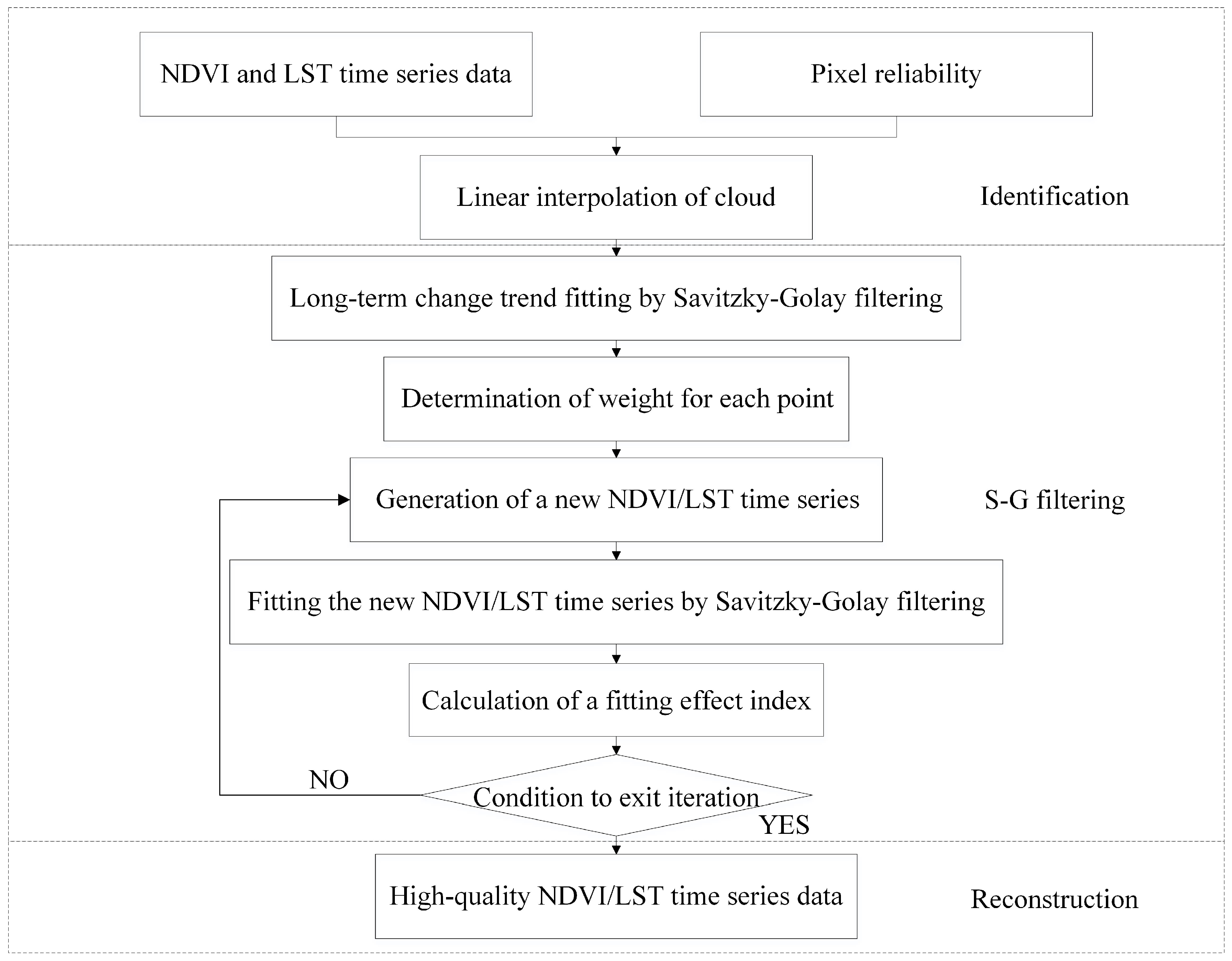
2.3. Savitzky–Golay (S-G) Filtering

MODIS data are affected by undetected clouds and poor atmospheric conditions, resulting in discontinuous data; thus, these data should be filtered [37,38]. The Savitzky–Golay (S-G) filtering method was proposed by Savitzky and Golay in 1964. This method smoothes and reconstructs a set of adjacent values or related spectral values by using the least squares algorithm, in order to reduce the errors or noises caused by undetected clouds and poor atmospheric conditions. S-G filtering can also be understood as a moving-window weighted averaging algorithm, taking each pixel in the study area as a unit, using a given high-order polynomial to fit the pixel values of each unit at different times, and reconstructing this set of data to compensate for the shortcomings of the data itself [39]. The formula for data processing by S-G filtering is as follows:
Y j * = i = m i = m C i Y j + 1 N
where Yj* is the reconstructed time series data; Y is the original time series data, Ci is the coefficient of filter fitting, i.e., the weight of the original time series data; N is the filter processing data length and is equal to the smoothing window size (2m+1); and m is the half-width of the smoothing window.
In this paper, we adopted S-G filtering to reconstruct the MODIS NDVI and land surface temperature (LST) data. In the process of data reconstruction, two parameters need to be set. The first parameter is m, the half-width of the smoothing window. The larger the value of m, the more smoothing is applied to the data. The second parameter is d, an integer specifying the degree of the smoothing polynomial. A smaller value of d will produce a smoother result, but may introduce larger deviation; a higher value of d will reduce the filter bias, and may ‘‘over fit’’ the data and give a noisier result [40]. The flowchart of the S-G filtering method is shown in Figure 2.

2.4. Data Processing

Monthly precipitation and temperature data from the 124 meteorological stations were obtained from the National Meteorological Information Center (NMIC) of the China Meteorological Administration. Spatio–temporal homogeneity tests, together with manual inspection and correction of the data, had been performed by the NMIC, and the monthly precipitation and temperature data of each meteorological station were reliable and of good quality during the research period (2000–2015). Monthly SPEI of each station were calculated using monthly precipitation and temperature data from the 124 meteorological stations. In this study, 10 spatial interpolation methods were compared to choose the best one (Table 3). These methods can be classified into four categories: Inverse Distance Weighting (IDW), Polynomial Interpolation (PI), Radial Basis Function (RBF), and Kriging Interpolation (KI). Spatial interpolation of SPEI, based on 99 randomly selected stations (i.e., 80% of the 124 stations), was performed using all of the interpolation methods to choose the best one. Then, the interpolated SPEI of the remaining 25 stations using each method were compared with the calculated SPEI. Cross-validation was used to compare and select the most suitable interpolation method by calculating the mean relative error (MRE), root-mean-square error (RMSE), and correlation coefficient (R). Through comparative analysis, the Ordinary Kriging method was found to be the most suitable interpolation method, having the lowest MRE (0.01), lowest RMSE (0.18), and highest R value (0.99). Hence, in this study, the raster dataset of the SPEI was interpolated into a spatial resolution of 1 km using the Ordinary Kriging interpolation method.
Vegetation index datasets based on remote sensing were derived from the monthly MOD13A3 data product with a spatial resolution of 1 km from the US National Aeronautics and Space Administration (NASA) website (https://ladsweb.nascom.nasa.gov), including the NDVI. Five tiles covering the YRB (h25v04, h26v04, h25v05, h26v05, and h27v05) were selected from 2000 to 2015. LST data were derived from the 8-day MOD11A2 data product with a spatial resolution of 1 km, and were composed by Maximum Value Composite (MVC). The NDVI involves bands 1 and 2 of MODIS, and LST involves bands 20, 22, 23, 29, and 31–33 of MODIS. Quality control was performed according to the MOD13 User’s Guide (see: https://lpdaac.usgs.gov/sites/default/files/public/product_documentation/mod13_user_guide.pdf) and the MOD11 User’s Guide (see: https://lpdaac.usgs.gov/sites/default/files/public/product_documentation/mod11_user_guide.pdf).
In this paper, we used the S-G filtering method to reconstruct MODIS NDVI and LST data for improving data quality. First, the MODIS Reprojection Tool (MRT) was used to deal with MODIS images by batch-processing splicing, re-projecting, and clipping, and obtained the NDVI and LST for the general scope of the YRB. Then, combined with the vector layer of the YRB, batch cutting was carried out in ArcMap10.2 to obtain the monthly NDVI and LST data. Finally, NDVI and LST time series data were reconstructed based on S-G filtering, and the final filtered NDVI and LST were obtained. On the basis of the formula of VCI, TCI, VHI, and NVSWI, the monthly values of VCI, TCI, VHI, and NVSWI in the YRB were obtained by band math in ENVI. Based on the NDVI and LST, IDL programming was adopted in order to extract the LST value corresponding to the NDVI, and an NDVI–LST feature space scatter-plot was obtained. The maximum and minimum LST values corresponding to each NDVI value can be obtained, which were the dry and wet edges, and the monthly MTVDI can be obtained by fitting the dry and wet edges equation. Filtered monthly, NDVI and LST with a spatial resolution of 1 km were used to calculate all the monthly RSDIs (VCI, TCI, VHI, MTVDI, and NVSWI) (see formulas in Table 1), with an identical spatial resolution of 1 km. In this way, the temporal and spatial resolutions of all the remote sensed datasets are identical, and can be compared with the interpolated SPEI dataset.

2.5. Statistical methods

2.5.1. Extreme-Point Symmetric Mode Decomposition (ESMD)

Extreme-Point Symmetric Mode Decomposition (ESMD) is the latest development of the Hilbert–Huang transform. ESMD draws on the ideas of Empirical Mode Decomposition (EMD) and can be used in the fields of information science, marine and atmospheric science, ecology, and all other scientific studies involving data processing [41]. It uses the least squares method for optimizing the last remaining mode to become the entire data “adaptive global mean line” in order to obtain the optimal screening number. ESMD is an innovative method for obtaining the overall variation situation of time series, and can decompose the original time series into a series of IMF components and a trend item. The detailed decomposition process is described in Reference [42].

2.5.2. The Modified Mann–Kendall (MMK) trend test method

The Mann–Kendall (MK) trend test method is a nonparametric statistical test method to detect the trend change of time series. The prerequisite of the MK method is that the time series is assumed to be random and independent. However, the time series often has autocorrelation, which influences the significance of the test results. However, the Modified Mann–Kendall (MMK) trend test method can eliminate the autocorrelation components in the sequence and improve the testing ability of the MK method [43]. The detailed steps of the MMK method are described in Reference [44] and Reference [45].

2.5.3. Skill Score (SS)

Ordinary statistical methods such as average deviation, root-mean-square error, and correlation coefficient are used to evaluate the capability of various RSDIs. In this paper, we not only consider these ordinary methods, but also use a composite indicator (SS), considering deviation and correlation coefficient comprehensively, to evaluate the capability of different RSDIs elaborately and systematically [46]. The detailed steps are as follows:
Assuming that Yt and Xt are the time series of remotely sensed and meteorological drought grade results, respectively, the square error of remotely sensed and meteorological drought time series is defined as:
M S E ( y , x ) = 1 n t = 1 n ( Y t X t ) 2  
where n is the length of the time series. Through the non-dimensionalization of the above formula, the dimensionless SS can be calculated as follows:
S S = 1 M S E ( y , x ) M S E ( x ¯ , x ) = r y , x 2 [ r y , x ( s y / s x ) ] 2 [ ( y ¯ x ¯ ) / s x ] 2
where r y , x 2 is the square of the correlation coefficient between the remotely sensed and meteorological drought sequence, s y and s x are the standard deviations of the remotely sensed and meteorological drought sequence, respectively, and y ¯ and x ¯ are the average values of the remotely sensed and meteorological drought sequence, respectively. The greater the correlation coefficient of the remotely sensed and meteorological drought grade results, and the smaller the deviation, the closer the results of the remotely sensed and meteorological drought (SS is close to 1). Otherwise, the SS is smaller (<1).

3. Results

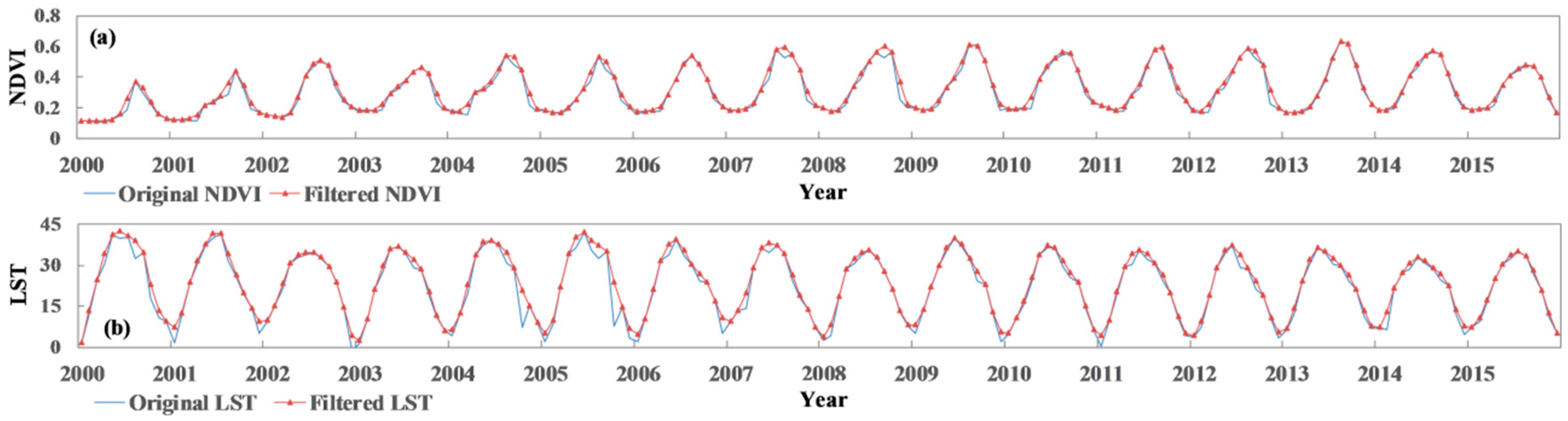
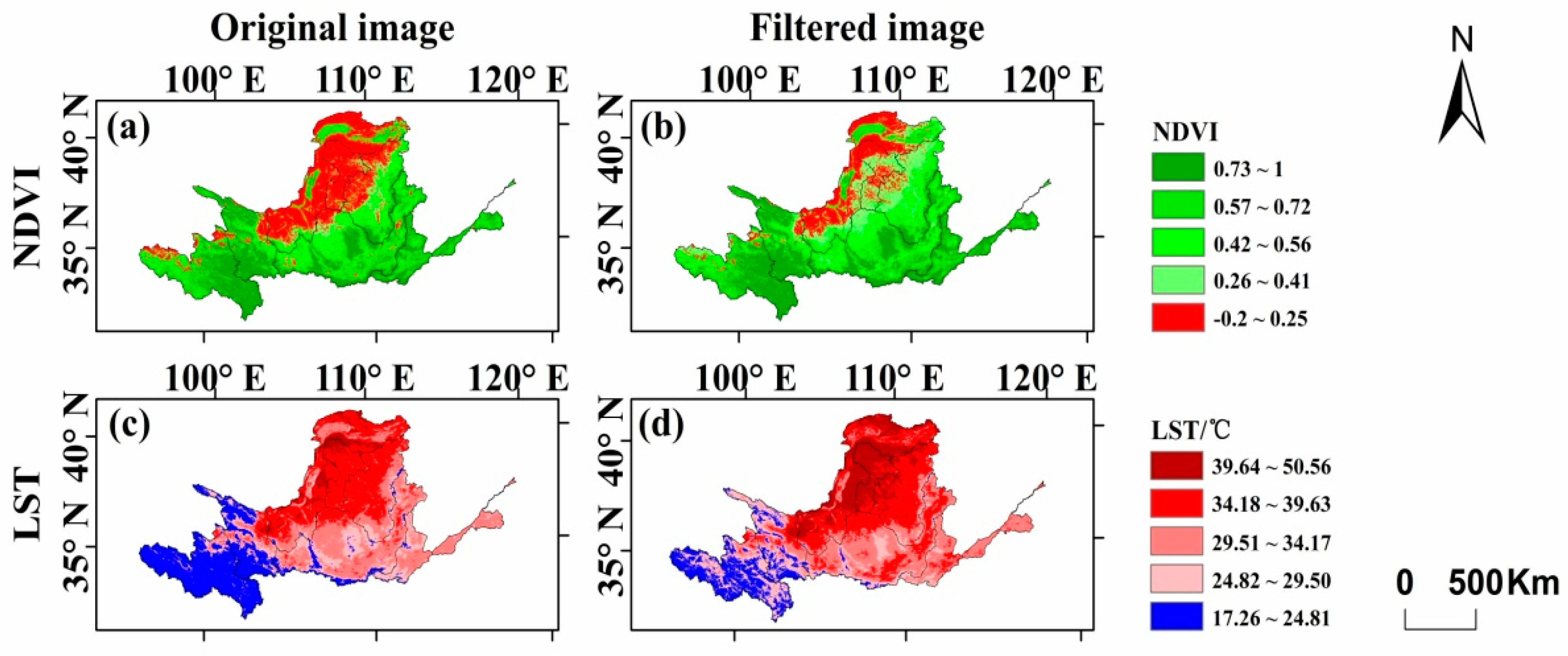
3.1. Reconstruction of NDVI and LST time series data

To minimize the possible impacts of undetected clouds and poor atmospheric conditions, S-G filtering was used to reconstruct the MODIS NDVI and LST time series data for the YRB during 2000–2015. The program achieved the best fitting effect after 10 iterations, and the filter parameters were set to m = 2, d = 3. The NDVI and LST profiles of one randomly selected pixel is shown in Figure 3. The pixel is located in the IF of the YRB with the land cover type of grassland. Theoretically, the inter-annual variation of NDVI and LST curves should be continuous and smooth. From the original NDVI and LST curves of the verification point, it can be seen that the time series were not very smooth, with a sudden drop occurring in some periods. The original NDVI and LST of the sudden drop were attributed to cloud and snow pixels, which resulted in sudden descent points (noises) that were inconsistent with the overall trend. After filtering, the values lower than the overall trend were considered as noise points, and were replaced by the filtering results, while the values higher than the overall trend were considered as normal values and were reserved. The NDVI and LST curves were obviously smoothed after S-G filtering, and the values marked as noise had been improved (Figure 3). The final curves were in accordance with the gradual variation trend of the NDVI and LST.
Figure 4 shows a comparison of the original and filtered images of NDVI and LST in July 2010. The good data in the original image can be retained to ensure the accuracy of the reconstructed image. The noise points were replaced by the new pixel values, and the difference of each pixel between the filtered and original image was greater than or equal to zero. From Figure 4, it can be seen that the NDVI in IF and the LST in AL were obviously improved. The data reconstructed by S-G filtering were significantly improved, as compared with the original data, and the filtered image can represent the real information of NDVI and LST. S-G filtering can effectively compensate for the data error caused by undetected clouds and poor atmospheric conditions, thus improving the quality of MODIS NDVI and LST time series data.

3.2. Temporal and spatial characteristics of drought

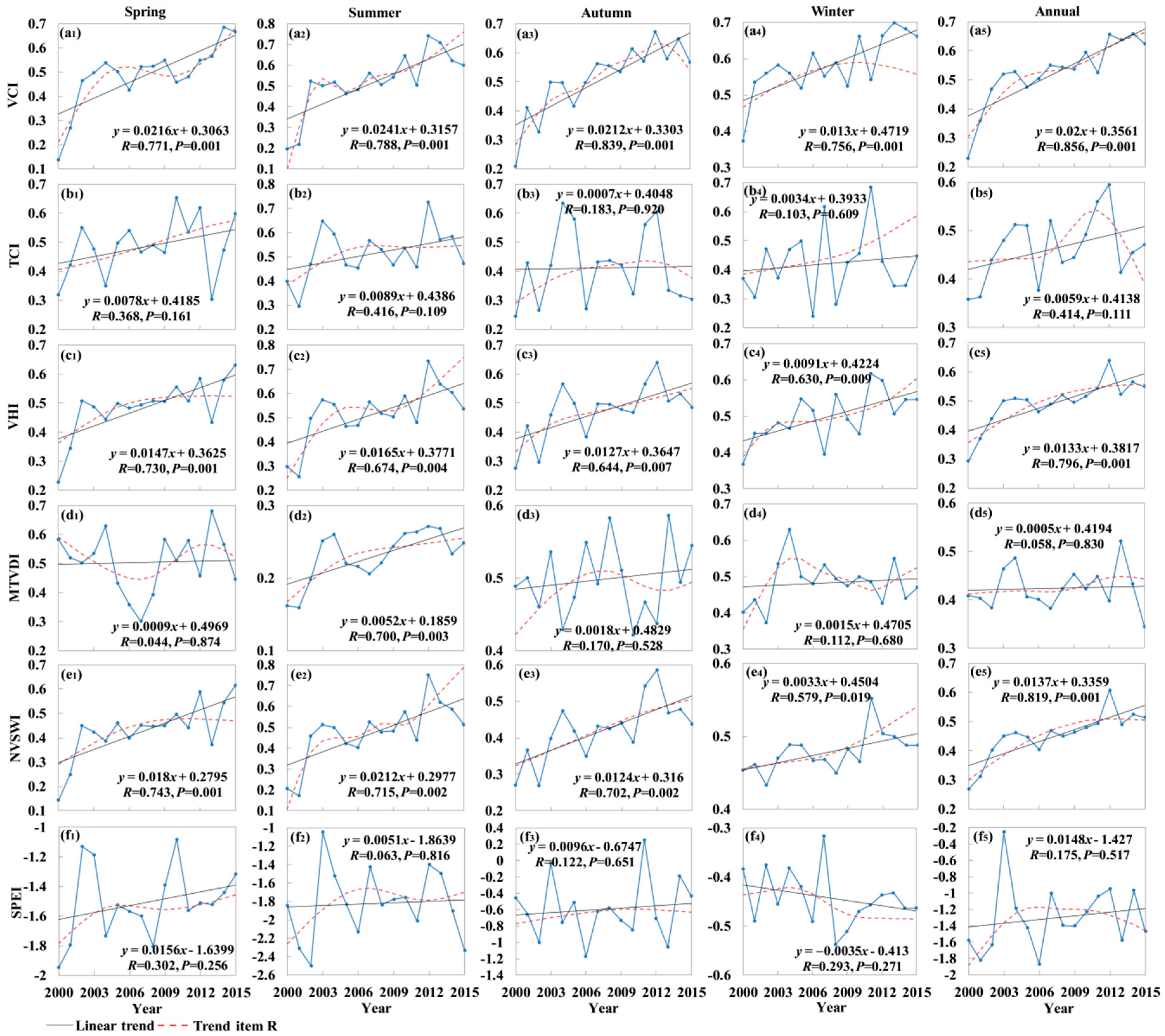
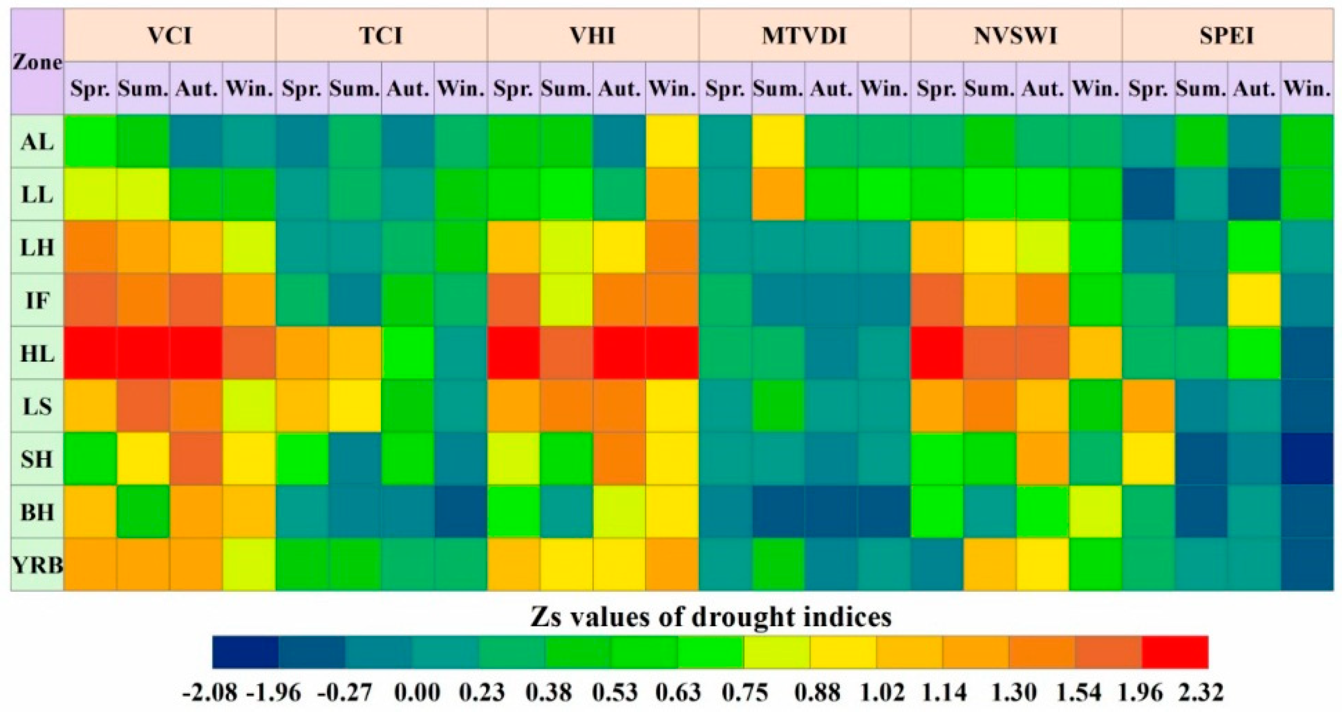
3.2.1. Temporal characteristics

In order to explore the overall drought variation in the YRB from 2000 to 2015, the RSDIs (VCI, TCI, VHI, MTVDI, and NVSWI) and the meteorological drought index (SPEI) were decomposed, respectively, using ESMD. The ESMD decomposition automatically stopped with trend item R corresponding to the minimum variance ratio, and the long-term overall variation trend of drought could be obtained (Figure 5). The trend item R based on ESMD decomposition can reflect the overall variation trend of drought, which was the adaptive global average line of the sequence. The variation trends of different drought indices clearly varied. The linear tendency rates of the annual VCI, TCI, VHI, MTVDI, NVSWI, and SPEI were 0.2/10a, 0.059/10a, 0.133/10a, 0.005/10a, 0.137/10a, and 0.148/10a, with the most obvious increasing trend being observed in the VCI. The remotely sensed and meteorological drought index showed an upward trend during 2000–2015, indicating that the drought in the YRB was slowing down on the annual scale. On the seasonal scale, the agricultural drought in each season, based on remote sensing, showed a downward trend, with the most obvious decreasing trend of drought being observed in summer. The linear tendency rates of VCI, TCI, VHI, MTVDI, and NVSWI in summer was 0.241/10a, 0.089/10a, 0.165/10a, 0.052/10a, and 0.212/10a, respectively. The average SPEIs for spring, summer, autumn, and winter were −1.51, −2.03, −0.59, and −0.44, respectively. The most severe season for meteorological drought was summer, followed by spring. The smaller the SPEI value was, the heavier the drought was; that is, a downward trend of SPEI indicates that drought is increasing. The tendency rate of winter SPEI was −0.035/10a, indicating that meteorological drought was increasing in winter. This shows that, although meteorological drought occurred, agricultural drought was not necessarily occurring due to agricultural irrigation and other field management measures.

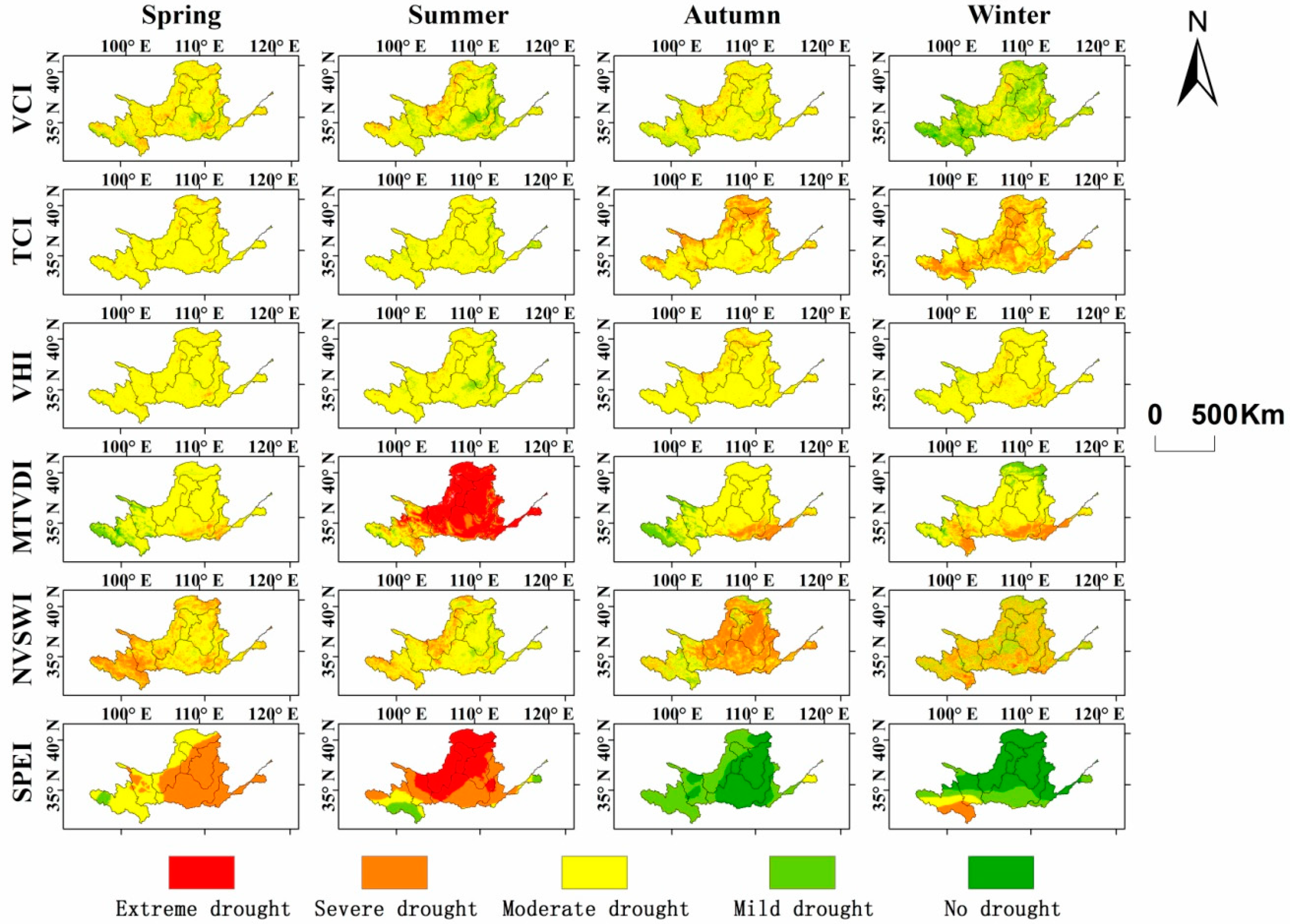
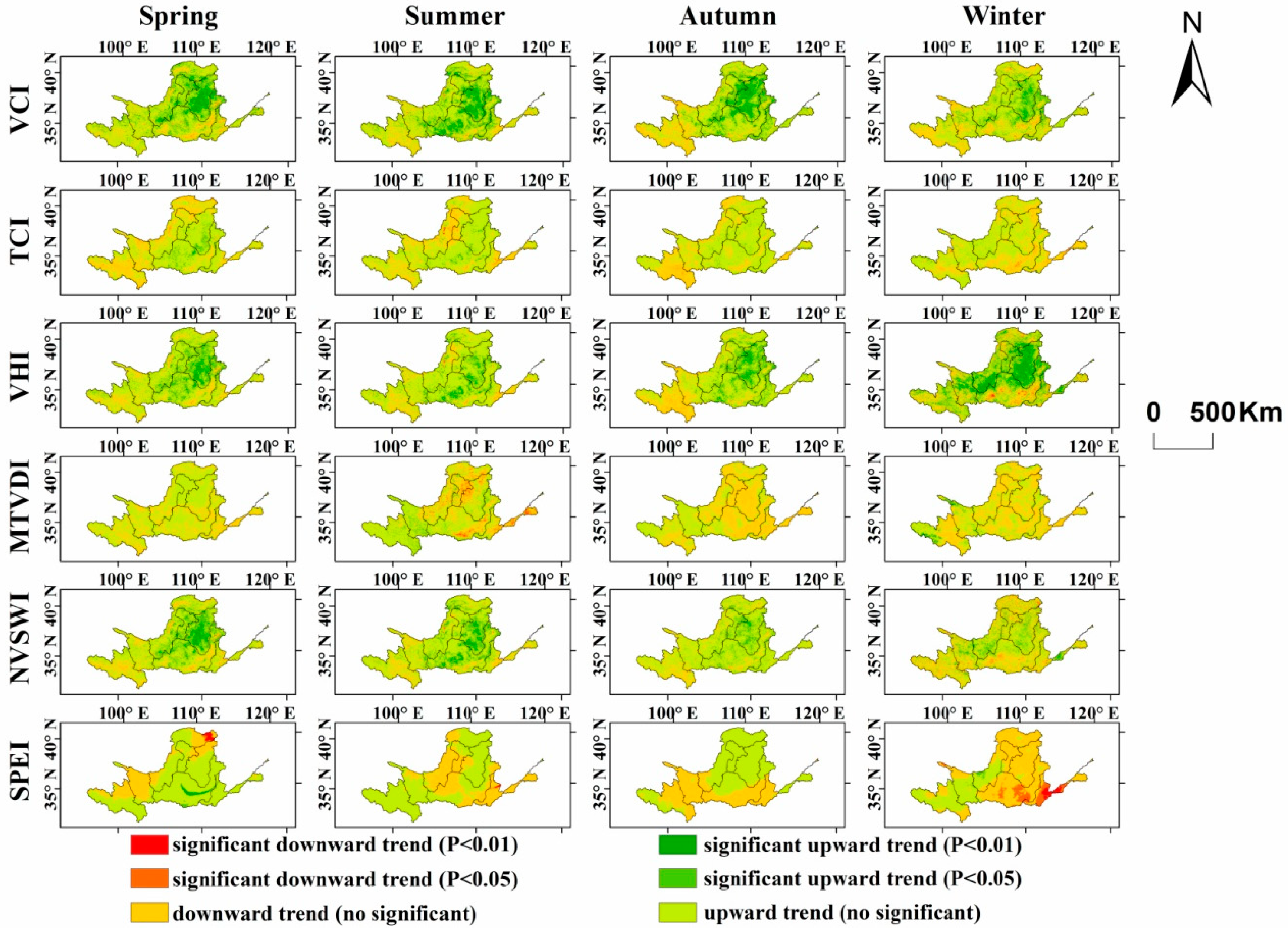
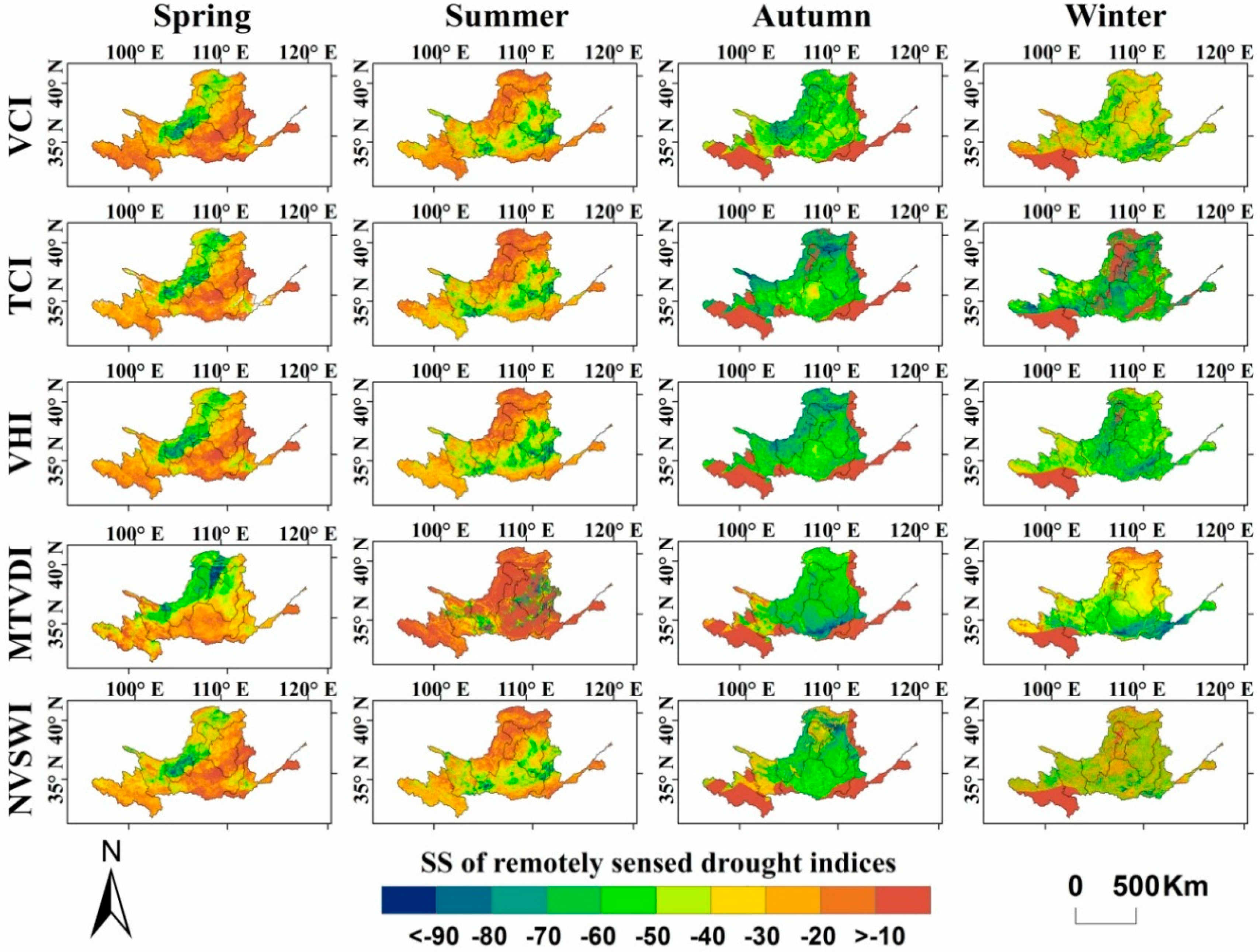
3.2.2. Spatial distribution

The drought spatial distribution characteristics of the YRB were obtained after the drought classification monitored by remotely sensed and meteorological drought index (Figure 6). In spring, the percentage of areas with moderate drought monitored by VCI, TCI, VHI, MTVDI, NVSWI, and SPEI was 81.6%, 95.5%, 96.3%, 85.2%, 65.8%, and 38.3%, respectively, and the percentage of areas with severe drought (59.4%) was also higher—monitored by the SPEI. With the increase of temperature in summer, extreme drought occurred in most areas monitored by the MTVDI and SPEI, with area percentages of 63.2% and 48.2%, respectively. The percentage of areas with moderate drought monitored by VCI, TCI, VHI, and NVSWI was 75.7%, 93.7%, 91.9%, and 79.6%, respectively. In autumn, the percentage of areas with moderate drought monitored by the VCI, TCI, VHI, MTVDI, and NVSWI was 84.8%, 75.8%, 94.3%, 78.2%, and 39.2%, respectively, while the percentage of areas with mild drought monitored by SPEI (48.3%) was also higher. The TCI and NVSWI also detected severe drought in some areas, with the percentage of areas with severe drought detected by NVSWI (52.1%) being higher than that detected by TCI (24.2%). In winter, the percentage of areas with moderate drought monitored by the VCI, TCI, VHI, MTVDI, and NVSWI was 53.1%, 61.6%, 92.9%, 70.9%, and 47.2%, respectively; conversely, most areas experienced no drought, as monitored by SPEI, which detected an area percentage of 62.7%. The VCI and TCI also detected mild drought and severe drought, respectively, giving area percentages of 41.9% and 38.1%, respectively.
From the drought grade results, it can be seen that the main drought type was moderate drought as monitored by different RSDIs in the YRB. The TCI and NVSWI in autumn, and the TCI in winter, detected severe drought in the YRB. The MTVDI in summer, and the VCI in winter, detected extreme drought and mild drought, respectively. The grade results of meteorological drought indicated that meteorological drought was more serious in spring (severe drought) and summer (extreme drought), and less serious in autumn (mild drought) and winter (no drought).
The seasonal trends of drought indices in the YRB based on the MMK trend test method are shown in Figure 7 and Figure 8. The trend characteristic values of the VCI, TCI, VHI, MTVDI, NVSWI, and SPEI were 1.22, 0.50, 1.13, 0.19, 1.07, and 0.37 in spring; 1.24, 0.48, 0.96, 0.42, 1.05, and 0.04 in summer; 1.15, 0.34, 0.99, 0.06, 0.96, and 0.21 in autumn; and 0.87, 0.26, 1.25, 0.11, 0.58, and −0.39 in winter. Seasonal drought showed a decreasing trend based on remote sensing in the YRB. Among them, the Zs values of spring, summer, and autumn VCI, spring, autumn, and winter VHI, and spring NVSWI in HL all passed the significance test of α = 0.05, which indicated that drought in these regions was significantly slowing down, as monitored by these indices. Based on the SPEI, the meteorological drought showed a decreasing trend in spring, summer, and autumn, and an increasing trend in winter (Zs = −0.39) in the YRB. The trend characteristic value of each subzone was slightly different; the Zs value of winter SPEI passed the significance test of α = 0.05 in SH, which showed that the meteorological drought in this region increased significantly in winter.

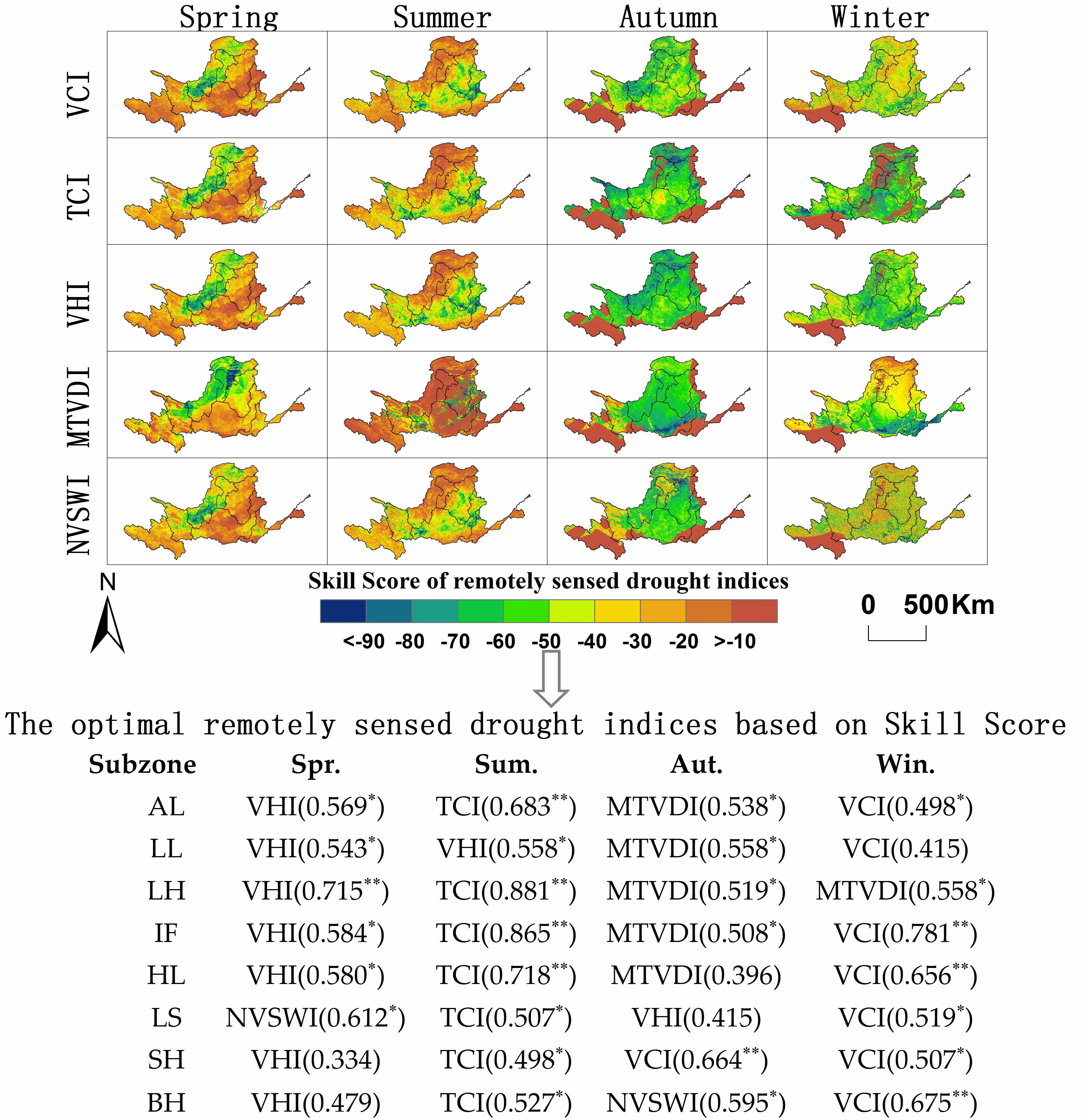
3.3. Capability of remotely sensed drought indices

This paper compared the grade results of remotely sensed and meteorological drought in order to quantitatively explore the capability of RSDIs in the YRB. The spatial distribution of SS was used to reflect the correlation coefficient and deviation information between remotely sensed and meteorological drought. The optimal RSDIs with high accuracy under different temporal and spatial patterns were selected by using optimal strategy in order to improve the accuracy of remotely sensed drought monitoring in the YRB.
Based on the classification standard of drought indices (Table 2), the spatial distribution of remotely sensed and meteorological drought grade results were obtained. The grade results of the meteorological drought index (SPEI) were considered as reference values, the grade results of RSDIs (VCI, TCI, VHI, MTVDI, and NVSWI) were considered as evaluation values, and the SS of the RSDIs were calculated (Figure 9). The greater the SS value, the higher the accuracy of Remotely Sensed Drought Index (RSDI). The average SS value of all pixels was calculated in each subzone of the YRB and the optimal RSDI with the maximum SS value in a specific season of each subzone was obtained (Table 4). In spring, the optimal RSDI of seven subzones was the VHI. In summer, the optimal RSDI of seven subzones was the TCI. In autumn, the optimal RSDI of five subzones was the MTVDI. In winter, the optimal RSDI of seven subzones was the VCI. As mentioned above, the optimal RSDI in spring, summer, autumn, and winter was the VHI, TCI, MTVDI, and VCI, respectively.
A total of 18 optimal drought indices passed the significance test of α = 0.05 and nine optimal drought indices passed the significance test of α = 0.01. The proportion of optimal drought indices reached 84.4%, which passed the significance test. The average correlation coefficient was 0.577, which passed the significance test of α = 0.05. It can be seen that the correlation coefficient of drought grade results between the agricultural drought based on the optimal RSDIs and meteorological drought based on SPEI was higher. In view of the fact that the SS was a dimensionless indicator, which took into account correlation coefficient and deviation, the evaluation result was more comprehensive and objective. In future research, we should adopt these optimal RSDIs based on SS to monitor drought in the YRB in order to provide a scientific and rational assessment of drought conditions and provide reference and basis for the formulation of drought relief measures.

4. Discussion

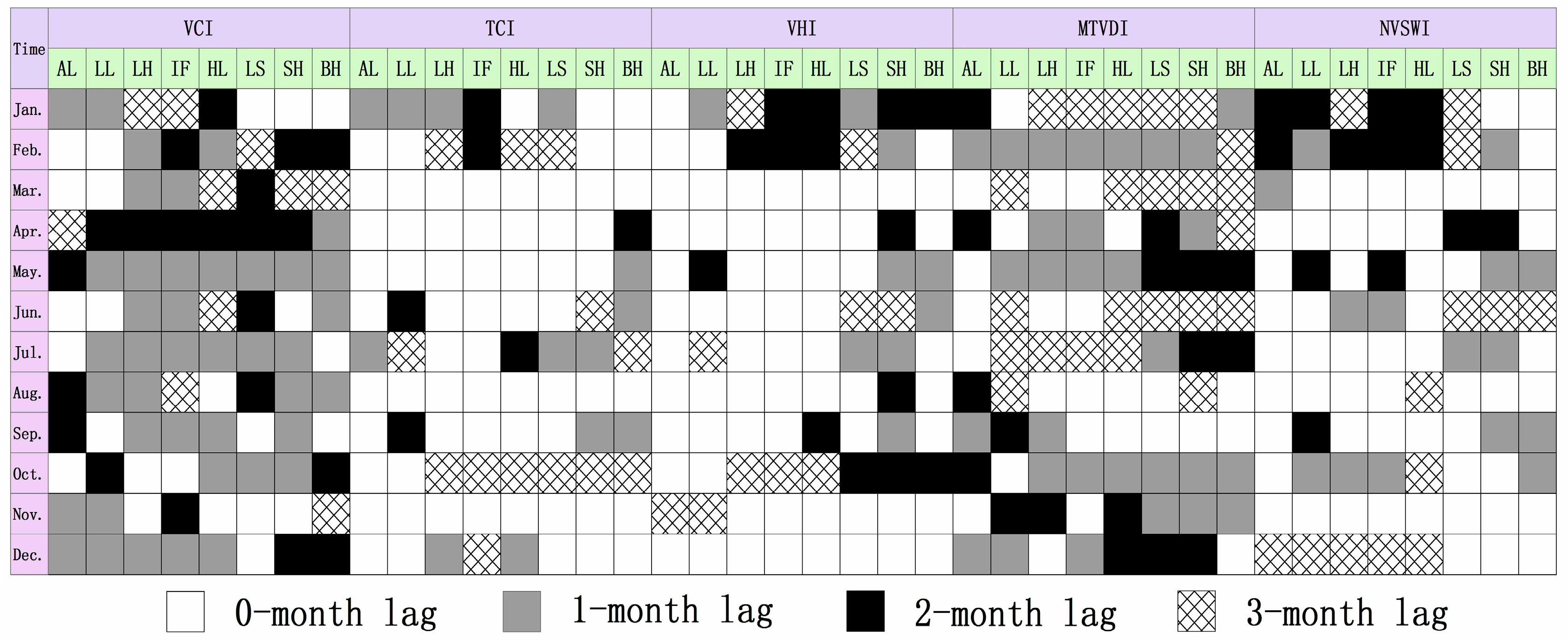
4.1. Hysteresis analysis

The results of remotely sensed drought showed different delayed responses to meteorological drought with a certain time lag [47]. In order to quantitatively investigate the hysteresis of remotely sensed drought monitoring results relative to meteorological drought results, this paper delayed the drought results of RSDIs for zero to three months (zero-month lag, one-month lag, two-month lag, and three-month lag) so as to seek the optimal time-lag effect between remotely sensed and meteorological drought [48,49]. By comparing the average SS between meteorological drought and remotely sensed drought with a zero-month lag, one-month lag, two-month lag, and three-month lag, the time lags of RSDIs in each subzone were obtained (Figure 10). Remotely sensed drought monitored by VCI, TCI, VHI, MTVDI, and NVSWI had hysteresis relationships with meteorological drought, with different time-lags in each subzone. In January, the time lag of VCI was one month in AL and LL, three months in LH and IF, two months in HL, and zero months in LS, SH, and BH. The time lag of TCI was one month in AL, LL, LH, and LS, two months in IF, and zero months in HL, SH, and BH. The time lags of the other RSDIs are shown in Figure 10. Each RSDI had a time lag in different periods. This was because changes in vegetation greenness and moisture due to drought took time to accumulate and develop, which is in accordance with the result of Reference [50].

4.2. Drought evolution in the YRB

Drought occurrence has obvious temporal and spatial characteristics. The drought conditions were different when monitored by different RSDIs. On the annual scale, drought slowed down in the YRB during the 16-year study period, which is consistent with the previous research of References [51,52]. On the seasonal scale, the agricultural drought in each season showed a decreasing trend based on remote sensing, which was slightly different from the meteorological drought (which was aggravated in winter). The decreasing trend of precipitation (−3.88 mm/10a) and the increasing trend of temperature (0.18℃/10a) were more significant in winter; thus, winter was the only season when an increase in meteorological drought was observed (SPEI tendency rate of −0.035/10a), which was in agreement with the conclusion of the characteristic value of the MMK trend test (Zs < 0). While meteorological drought occurred, agricultural drought did not necessarily occur, due to agricultural irrigation and other field management measures [53]. If meteorological drought occurred with a long-term reduction in precipitation, the occurrence of agricultural drought depended on the time and location of meteorological drought and the local irrigation conditions and planting structure. If timely irrigation can be provided for crops after meteorological drought, or other agricultural measures can be taken to maintain soil moisture and meet crop demand, agricultural drought will not occur [25,54]. Furthermore, human activities can also affect the vegetation status of the YRB, thus affecting vegetation coverage and the development of agricultural drought. The YRB has always been the major region of ecological protection and construction in China. Since 2000, China has invested significant funds in ecological restoration. A large number of major ecological environmental protection and construction projects have been implemented, such as grain for green, returning pasture to grass, natural forest protection, and protective forest system engineering [55]. With the implementation of ecological engineering, the vegetation status of the YRB has been improved and the vegetation growth has an obvious increasing trend. Therefore, it was considered that agricultural drought tended to slow down in the YRB, which was the result of ecological protection and forest planting in large areas in recent years [56,57]. Besides forest planting, an increase in precipitation (19.88 mm/10a) was also one of the main causes of drought mitigation [58]. The characteristic of meteorological drought in each season was obviously different, with the highest average temperature being recorded in summer (20.08℃) and the second highest in spring (9.64℃). The most serious meteorological drought occurred in summer and spring. Liu et al. indicated that there was relatively large crop water demand in summer, and less rainfall in spring with great inter-annual variation, resulting in serious meteorological drought in summer and spring, which is consistent with the research results obtained in this study [59].

5. Conclusions

The capability of RSDIs should be fully considered under different spatio–temporal patterns, which can improve the accuracy of drought monitoring in the YRB. Based on the SS method, five RSDIs (VCI, TCI, VHI, MTVDI, and NVSWI) were quantitatively evaluated with the meteorological drought index SPEI in order to determine the optimal RSDIs under different spatio–temporal patterns from 2000 to 2015.
Drought slowed down in the YRB during 2000–2015. The linear tendency rates of the VCI, TCI, VHI, MTVDI, NVSWI, and SPEI were 0.2/10a, 0.059/10a, 0.133/10a, 0.005/10a, 0.137/10a, and 0.148/10a, with the most obvious trend being seen for the VCI. The main drought type was moderate drought, as monitored by different RSDIs in the YRB. On the seasonal scale, agricultural drought showed a decreasing trend based on the RSDIs, and meteorological drought showed a decreasing trend based on spring, summer, and autumn SPEI and an increasing trend based on winter SPEI. The drought results based on remote sensing were slightly different from the results obtained for meteorological drought, and had time lags of zero–three months compared with meteorological drought. By investigating the capability of RSDIs under different spatio–temporal patterns, the optimal RSDIs in spring, summer, autumn, and winter were found to be the VHI, TCI, MTVDI, and VCI, respectively, and the average correlation coefficient between the RSDIs and the SPEI was 0.577 (α = 0.05). In the future, the optimal RSDIs should be adopted to monitor drought conditions in the YRB, which can provide a reasonable scientific basis for relevant departments to plan and make decisions relating to drought.
In this study, we combined remotely sensed and meteorological drought indices to study the characteristics of drought and quantitatively evaluated the capability of RSDIs in the YRB. However, the factors involved in this paper were limited, and the physical mechanism of drought was not taken into account. There are many other factors involved in the occurrence of drought, and we should take these into account. Furthermore, we should increase the category of RSDIs to expand the scope of selection in future research, which is highly necessary for accurate drought monitoring.

Author Contributions

Haibo Yang and Yong Zhao formulated the problem and designed the experiments; Fei Wang analyzed the data and performed the experiments. Zhenhong Li provided crucial guidance and support through the research. Fei Wang, Haibo Yang, Yong Zhao and Zongmin Wang contributed to the discussion and edited the manuscript. Fei Wang and Jiapeng Wu contributed to the validation work and data interpretation.

Funding

This research was supported by National Key R&D Program of China (2018YFC0406505), Henan Province Scientific and Technological Project (Grant Nos. 162102410066 & 172102410075), the Open Research Fund of the State Key Laboratory of Simulation and Regulation of Water Cycle in River Basin at the China Institute of Water Resources and Hydropower Research (IWHR-SKL-201701), and Science and technology project of Guizhou Province Water Resources Department (KT201705). The work was also supported by the UK National Environment Research Council (NERC) through the Drier-China project (ref.: NE/P015484/1) and the UK Science and Technology Facilities Council (STFC) through the PAFiC project (ref.: ST/N006801/1).

Acknowledgments

Thanks to Enchong Li for data collection and arrangement.

Conflicts of Interest

The authors declare no conflict of interest.

References

  1. Huang, S.Z.; Chang, J.X.; Leng, G.Y.; Huang, Q. Integrated index for drought assessment based on variable fuzzy set theory: A case study in the Yellow River Basin, China. J. Hydrol. 2015, 527, 608–618. [Google Scholar] [CrossRef]
  2. Yao, J.Q.; Zhao, Y.; Chen, Y.N.; Yu, X.J.; Zhang, R.B. Multi-scale assessments of droughts: A case study in Xinjiang, China. Sci. Total Environ. 2018, 630, 444–452. [Google Scholar] [CrossRef] [PubMed]
  3. Yao, N.; Li, Y.; Lei, T.J.; Peng, L.L. Drought evolution, severity and trends in mainland China over 1961–2013. Sci. Total Environ. 2017, 616, 73–89. [Google Scholar] [CrossRef] [PubMed]
  4. Yang, P.; Xia, J.; Zhang, Y.Y.; Zhan, C.S.; Qiao, Y.F. Comprehensive assessment of drought risk in the arid region of Northwest China based on the global palmer drought severity index gridded data. Sci. Total Environ. 2018, 627, 951–962. [Google Scholar] [CrossRef] [PubMed]
  5. Xia, L.; Zhao, F.; Mao, K.B.; Yuan, Z.J.; Zuo, Z.Y.; Xu, T.R. SPI-based analyses of drought changes over the past 60 years in China’s major crop-growing areas. Remote Sens. 2018, 10, 171. [Google Scholar] [CrossRef]
  6. Palmer, W.C. Meteorological Drought Research Paper 45; US Weather Bureau: Washington, DC, USA, 1965.
  7. Mckee, T.B.; Doesken, N.J.; Kleist, J. The relationship of drought frequency and duration to time scales. Am. Meteorol. Soc. 1993, 58, 174–184. [Google Scholar]
  8. Lopez-Moreno, J.I.; Vicente-Serrano, S.M.; Zabalzaa, J.; Beguería, S.; Lorenzo-Lacruz, J.; Azorin-Molina, C.; Morán-Tejeda, E. Hydrological response to climate variability at different time scales: A study in the Ebro basin. J. Hydrol. 2013, 477, 175–188. [Google Scholar] [CrossRef] [Green Version]
  9. Dorjsuren, M.; Liou, Y.A.; Cheng, C.H. Time series MODIS and in situ data analysis for Mongolia drought. Remote Sens. 2016, 8, 509. [Google Scholar] [CrossRef]
  10. Islam, M.M.; Shamsuddoha, M. Coastal and marine conservation strategy for Bangladesh in the context of achieving blue growth and sustainable development goals (SDGs). Environ. Sci. Policy. 2018, 87, 45–54. [Google Scholar] [CrossRef]
  11. Salvia, A.L.; Filho, W.L.; Brandli, L.L.; Griebeler, J.S. Assessing research trends related to Sustainable Development Goals: local and global issues. J. Clean. Prod. 2019, 208, 841–849. [Google Scholar] [CrossRef]
  12. Winkler, K.; Gessner, U.; Hochschild, V. Identifying droughts affecting agriculture in Africa based on remote sensing time series between 2000–2016: rainfall anomalies and vegetation condition in the context of ENSO. Remote Sens. 2017, 9, 831. [Google Scholar] [CrossRef]
  13. Wu, D.; Qu, J.J.; Hao, X.J. Agricultural drought monitoring using MODIS-based drought indices over the USA Corn Belt. Int. J. Remote Sens. 2015, 36, 5403–5425. [Google Scholar] [CrossRef]
  14. Cong, D.M.; Zhao, S.H.; Chen, C.; Duan, Z. Characterization of droughts during 2001-2014 based on remote sensing: A case study of Northeast China. Ecol. Inform. 2017, 39, 56–67. [Google Scholar] [CrossRef]
  15. Kogan, F.N. Droughts of the late 1980s in the United States as derived from NOAA polar-orbiting satellite data. B. Am. Meteorol. Soc. 1995, 76, 655–668. [Google Scholar] [CrossRef]
  16. Zambrano, F.; Lillo-Saavedra, M.; Verbist, K.; Lagos, O. Sixteen years of agricultural drought assessment of the BioBío region in Chile using a 250 m resolution Vegetation Condition Index (VCI). Remote Sens. 2016, 8, 530. [Google Scholar] [CrossRef]
  17. Kogan, F.N. Application of vegetation index and brightness temperature for drought detection. Adv. Space Res. 1995, 15, 91–100. [Google Scholar] [CrossRef]
  18. Chang, S.; Wu, B.F.; Yan, N.; Davdai, B.; Nasanbat, E. Suitability assessment of satellite-derived drought indices for Mongolian Grassland. Remote Sens. 2017, 9, 650. [Google Scholar] [CrossRef]
  19. Sandholt, I.; Rasmussen, K.; Andersen, J. A simple interpretation of the surface temperature/vegetation index space for assessment of surface moisture status. Remote Sens. Environ. 2002, 79, 213–224. [Google Scholar] [CrossRef]
  20. Wang, P.X.; Gong, J.Y.; Li, X.W. Vegetation-Temperature condition index and its application for drought monitoring. Geomat. Inform. Sci. Wuhan Univ. 2001, 26, 412–418. (In Chinese) [Google Scholar]
  21. Abbas, S.; Nichol, J.E.; Qamer, F.M.; Xu, J.C. Characterization of drought development through Remote Sensing: A case study in Central Yunnan, China. Remote Sens. 2014, 6, 4998–5018. [Google Scholar] [CrossRef] [Green Version]
  22. Nichol, J.E.; Abbas, S. Integration of remote sensing datasets for local scale assessment and prediction of drought. Sci. Total Environ. 2015, 505, 503–507. [Google Scholar] [CrossRef] [PubMed]
  23. Wang, X.W.; Liu, M.; Liu, L. Responses of MODIS spectral indices to typical drought events from 2000 to 2012 in southwest China. J. Remote Sens. 2014, 18, 432–452. [Google Scholar]
  24. Klisch, A.; Atzberger, C. Operational drought monitoring in Kenya using MODIS NDVI time series. Remote Sens. 2016, 8, 267. [Google Scholar] [CrossRef]
  25. Zhang, L.F.; Jiao, W.Z.; Zhang, H.M.; Huang, C.P.; Tong, Q.X. Studying drought phenomena in the Continental United States in 2011 and 2012 using various drought indices. Remote Sens. Environ. 2017, 190, 96–106. [Google Scholar] [CrossRef]
  26. Hao, C.; Zhang, J.H.; Yao, F.M. Combination of multi-sensor remote sensing data for drought monitoring over Southwest China. Int J Appl Earth Obs. 2015, 35, 270–283. [Google Scholar] [CrossRef]
  27. Du, L.T.; Tian, Q.J.; Yu, T.; Meng, Q.Y.; Jancso, T.; Udvardy, P.; Huang, Y. A comprehensive drought monitoring method integrating MODIS and TRMM data. Int J Appl Earth Obs. 2013, 23, 245–253. [Google Scholar] [CrossRef]
  28. Zhang, J.; Mu, Q.Z.; Huang, J.X. Assessing the remotely sensed drought severity index for agricultural drought monitoring and impact analysis in North China. Ecol. Indic. 2016, 63, 296–309. [Google Scholar] [CrossRef]
  29. Zhang, X.; Wei, C.H.; Obringer, R.; Li, D.; Chen, N.C.; Niyogi, D. Gauging the severity of the 2012 Midwestern U.S. drought for agriculture. Remote Sens. 2017, 9, 767. [Google Scholar] [CrossRef]
  30. Pierce, D.W.; Barnett, T.P.; Santer, B.D.; Gleckler, P.J. Selecting global climate models for regional climate change studies. Proc. Natl. Acad. Sci. 2009, 106, 8441–8446. [Google Scholar] [CrossRef] [PubMed] [Green Version]
  31. Liu, Y.; Wu, Y.Z.; Feng, Z.Z.; Huang, X.R.Z.; Wang, D.G. Evaluation of a variety of satellite retrieved precipitation products based on extreme rainfall in China. Trop. Geogr. 2017, 37, 417–433. (In Chinese) [Google Scholar]
  32. Chen, W.L.; Jiang, Z.H.; Li, L. Probabilistic projections of climate change over China under the SRES A1B scenario using 28 AOGCMs. J. Climate. 2011, 24, 4741–4756. [Google Scholar] [CrossRef]
  33. Zhang, B.Q.; He, C.S.; Morey, B.; Zhang, L.H. Evaluating the coupling effects of climate aridity and vegetation restoration on soil erosion over the Loess Plateau in China. Sci. Total Environ. 2016, 539, 436–449. [Google Scholar] [CrossRef] [PubMed]
  34. Jiang, S.H.; Zhou, M.; Ren, L.L.; Cheng, X.R.; Zhang, P.J. Evaluation of latest TMPA and CMORPH satellite precipitation products over Yellow River Basin. Water Sci. Eng. 2016, 9, 87–96. [Google Scholar] [CrossRef]
  35. Zhao, H.Y.; Gao, G.; An, W.; Zou, X.K.; Li, H.T.; Hou, M.T. Timescale differences between SC-PDSI and SPEI for drought monitoring in China. Phys. Chem. Earth. 2015, 10, 1–11. [Google Scholar] [CrossRef]
  36. Zhang, B.Q.; Zhao, X.N.; Jin, J.M.; Wu, P. Development and evaluation of a physically based multiscalar drought index: The Standardized Moisture Anomaly Index. J. Geophys. Res. 2015, 120, 11575–11588. [Google Scholar] [CrossRef]
  37. Beck, P.S.A.; Atzberger, C.; Høgda, K.A.; Johansen, B.; Skidmore, A.K. Improved monitoring of vegetation dynamics at very high latitudes: A new method using MODIS NDVI. Remote Sens. Environ. 2005, 100, 321–334. [Google Scholar] [CrossRef]
  38. Vuolo, F.; Ng, W.T.; Atzberger, C. Smoothing and gap-filling of high resolution multi-spectral time series: Example of Landsat data. Int J Appl Earth Obs. 2017, 57, 202–213. [Google Scholar] [CrossRef]
  39. Savitzky, A.; Golay, M.J.E. Smoothing and differentiation of data by simplified least squares procedures. Anal. Chem. 1964, 36, 1627–1639. [Google Scholar] [CrossRef]
  40. Chen, J.; Jönsson, P.; Tamura, M.; Gu, Z.H.; Matsushita, B.; Eklundh, L. A simple method for reconstructing a high-quality NDVI time-series dataset based on the Savitzky–Golay filter. Remote Sens. Environ. 2004, 91, 332–344. [Google Scholar] [CrossRef]
  41. Wang, J.L.; Li, Z.J. The ESMD method for climate data analysis. Clim. Change Res. Lett. 2014, 3, 1–5. [Google Scholar] [CrossRef]
  42. Li, H.F.; Wang, J.L.; Li, Z.J. Application of ESMD method to air-sea flux investigation. Int. J. Geos. 2013, 4, 8–11. [Google Scholar] [CrossRef]
  43. Huang, S.Z.; Chang, J.X.; Huang, Q.; Chen, Y.T. Spatio-temporal changes and frequency analysis of drought in the Wei River basin, China. Water Resour. Manag. 2014, 28, 3095–3110. [Google Scholar] [CrossRef]
  44. Tabari, H.; Talaee, P.H.; Nadoushani, S.S.M.; Willems, P.; Marchetto, A. A survey of temperature and precipitation based aridity indices in Iran. Quatern. Int. 2014, 345, 158–166. [Google Scholar] [CrossRef]
  45. Huang, S.Z.; Huang, Q.; Zhang, H.B.; Chen, Y.T.; Leng, G.Y. Spatio-temporal changes in precipitation, temperature and their possibly changing relationship: a case study in the Wei River Basin, China. Int. J. Climatol. 2016, 36, 1160–1169. [Google Scholar] [CrossRef]
  46. Jiang, Z.H.; Lu, Y.; Ding, Y.G. Analysis of the high-resolution merged precipitation products over China based on the temporal and spatial structure score indices. Acta. Meteorol. Sin. 2013, 71, 891–900. [Google Scholar]
  47. Potopová, V.; Štěpánek, P.; Možný, M.; Türkott, L.; Soukup, J. Performance of the standardised precipitation evapotranspiration index at various lags for agricultural drought risk assessment in the Czech Republic. Agr. Forest Entomol. 2015, 202, 26–38. [Google Scholar] [CrossRef]
  48. Caccamo, G.; Chisholm, L.A.; Bradstock, R.A.; Puotinen, M.L. Assessing the sensitivity of MODIS to monitor drought in high biomass ecosystems. Remote Sens. Environ. 2011, 115, 2626–2639. [Google Scholar] [CrossRef]
  49. Wang, H.S.; Lin, H.; Liu, D.S. Remotely sensed drought Index and its responses to meteorological drought in Southwest China. Remote Sens. Lett. 2014, 5, 413–422. [Google Scholar] [CrossRef]
  50. Ji, L.; Peters, A.J. Assessing vegetation response to drought in the northern Great Plains using vegetation and drought indices. Remote Sens Environ. 2003, 87, 85–98. [Google Scholar] [CrossRef]
  51. Yuan, L.H.; Jiang, W.G.; Shen, W.M.; Liu, Y.H.; Wang, W.J.; Tao, L.L.; Zheng, H.; Liu, X.F. The spatial-temporal variations of vegetation cover in the Yellow River Basin from 2000 to 2010. Acta. Ecol. Sin. 2013, 33, 7798–7806. (In Chinese) [Google Scholar]
  52. Zhao, Q.; Chen, Q.Y.; Jiao, M.Y.; Wu, P.T.; Gao, X.R.; Ma, M.H.; Hong, Y. The temporal-spatial characteristics of drought in the Loess Plateau using the remote-sensed TRMM precipitation data from 1998 to 2014. Remote Sens. 2018, 10, 838. [Google Scholar] [CrossRef]
  53. Tang, Y.; Sun, R. Drought characteristics in Henan province with meteorological and remote sensing data. J. Nat. Resour. 2013, 28, 646–655. (In Chinese) [Google Scholar]
  54. Pablos, M.; Martínez-Fernández, J.; Sánchez, N.; González-Zamora, Á. Temporal and spatial comparison of agricultural drought indices from moderate resolution satellite soil moisture data over Northwest Spain. Remote Sens. 2017, 9, 1168. [Google Scholar] [CrossRef]
  55. Zhang, Y.L.; Su, H.M.; Zhang, X.Y. The spatial-temporal changes of vegetation restoration in the Yellow River Basin from 1998 to 2012. J. Desert Res. 2014, 34, 597–602. (In Chinese) [Google Scholar]
  56. Jiang, W.G.; Yuan, L.H.; Wang, W.J.; Cao, R.; Zhang, Y.F.; Shen, W.M. Spatio-temporal analysis of vegetation variation in the Yellow River Basin. Ecol. Indic. 2015, 51, 117–126. [Google Scholar] [CrossRef]
  57. Gao, X.R.; Sun, M.; Zhao, Q.; Wu, P.T.; Zhao, X.N.; Pan, W.X.; Wang, Y.B. Actual ET modelling based on the Budyko framework and the sustainability of vegetation water use in the loess plateau. Sci. Total Environ. 2017, 579, 1550–1559. [Google Scholar] [CrossRef] [PubMed]
  58. Huang, S.Z.; Huang, Q.; Chang, J.X.; Zhu, Y.L.; Leng, G.Y.; Xing, L. Drought structure based on a nonparametric multivariate standardized drought index across the Yellow River basin, China. J. Hydrol. 2015, 530, 127–136. [Google Scholar] [CrossRef]
  59. Liu, Q.; Yan, C.R.; He, W.Q. Drought variation and its sensitivity coefficients to climatic factors in the Yellow River Basin. Chin. J. Agrometeorol. 2016, 37, 623–632. (In Chinese) [Google Scholar]
Figure 1. The study area and distribution of meteorological stations.
Remotesensing 10 01834 g001
Figure 2. Flowchart of Savitzky–Golay (S-G) Filtering Method.
Remotesensing 10 01834 g002
Figure 3. Original and filtered Normalized Difference Vegetation Index (NDVI) (a) and land surface temperature (LST) (b) time series.
Remotesensing 10 01834 g003
Figure 4. Original and filtered image comparisons of Normalized Difference Vegetation Index (NDVI) and land surface temperature (LST) in July 2010: (a) Original NDVI image; (b) Filtered NDVI image; (c) Original LST image; and (d) Filtered LST image.
Remotesensing 10 01834 g004
Figure 5. Characteristics of drought in the Yellow River basin (YRB) during 2000–2015.
Remotesensing 10 01834 g005
Figure 6. Spatial distribution of seasonal drought in the Yellow River basin (YRB).
Remotesensing 10 01834 g006
Figure 7. Seasonal trends of drought indices in the Yellow River basin (YRB) during 2000–2015.
Remotesensing 10 01834 g007
Figure 8. Zs values of drought indices during 2000–2015.
Remotesensing 10 01834 g008
Figure 9. Spatial distribution of Skill Score (SS) in the Yellow River basin (YRB).
Remotesensing 10 01834 g009
Figure 10. Time-lags of remotely sensed drought indices (RSDIs) in the Yellow River basin (YRB).
Remotesensing 10 01834 g010
Table 1. Descriptions of remotely sensed drought indices (RSDIs).
IndexRangeFormulaParameterSource
VCI[0,1] V C I = N D V I i N D V I m i n N D V I m a x N D V I m i n NDVIi is the NDVI value of a certain period, and NDVImax and NDVImin are the maximum and minimum NDVI values in multi-year dataset.[13]
TCI[0,1] T C I = L S T m a x L S T i L S T m a x L S T m i n LSTi is the LST value of a certain period, and LSTmax and LSTmin are the maximum and minimum LST values in multi-year dataset.[15]
VHI[0,1] V H I = a V C I + b T C I a and b are used to show the contributions of VCI and TCI to VHI. Here we assume that the contributions are equal (a = b = 0.5).[15]
MTVDI[0,1] M T V D I = L S T s m a x L S T s L S T s m a x L S T s m i n LSTs is the land surface temperature of an arbitrary pixel, and LSTsmin and LSTsmax are LST values on wet edge and dry edge. LSTsmin and LSTsmax are calculated by groups of points at the lower and upper limits of the scatterplots, where LSTsmin is the minimum LST for a given NDVI (wet edge), and LSTsmax is the maximum LST for a given NDVI (dry edge).[18]
NVSWI[0,1] N V S W I = V S W I i V S W I m i n V S W I m a x V S W I m i n VSWIi is the VSWI value of a certain period, VSWImax and VSWImin are the maximum and minimum VSWI values in multi-year dataset.[19]
Table 2. Classification of drought indices used in this study.
GradeClassificationVCITCIVHIMTVDINVSWISPEI
1No drought[0.8,1][0.8,1][0.8,1][0.8,1][0.8,1](−0.5,+∞)
2Mild drought[0.6,0.8)[0.6,0.8)[0.6,0.8)[0.6,0.8)[0.6,0.8)(−1, −0.5]
3Moderate drought[0.4,0.6)[0.4,0.6)[0.4,0.6)[0.4,0.6)[0.4,0.6)(−1.5, −1]
4Severe drought[0.2,0.4)[0.2,0.4)[0.2,0.4)[0.2,0.4)[0.2,0.4)(−2,−1.5]
5Extreme drought[0,0.2)[0,0.2)[0,0.2)[0,0.2)[0,0.2)(−∞, −2]
Table 3. Comparison of different interpolation methods.
Interpolation methodsMRERMSER
Inverse Distance WeightingIDW1.111.050.91
Polynomial InterpolationGlobal PI2.601.750.71
Local PI1.491.090.90
Radial Basis FunctionCompletely Regularized Spline0.030.190.99
Spline With Tension0.030.190.99
Multiquadric Spline0.040.210.99
Inverse Multiquadric Spline0.030.190.99
Thin Plate Spline0.030.190.99
Kriging InterpolationOrdinary Kriging0.010.180.99
Universal Kriging1.871.350.84
Table 4. The optimal remotely sensed drought indices (RSDIs) in various subzones. Spr., Sum., Aut., and Win. denote spring, summer, autumn, and winter, respectively. The values in parentheses are the correlation coefficients of drought grade results between the optimal index and the Standardized Precipitation Evapotranspiration Index (SPEI). “” means significance at the 95% confidence level and “∗∗” means significance at the 99% confidence level.
SubzoneSpr.Sum.Aut.Win.
ALVHI(0.569)TCI(0.683∗∗)MTVDI(0.538)VCI(0.498)
LLVHI(0.543)VHI(0.558)MTVDI(0.558)VCI(0.415)
LHVHI(0.715∗∗)TCI(0.881∗∗)MTVDI(0.519)MTVDI(0.558)
IFVHI(0.584)TCI(0.865∗∗)MTVDI(0.508)VCI(0.781∗∗)
HLVHI(0.580)TCI(0.718∗∗)MTVDI(0.396)VCI(0.656∗∗)
LSNVSWI(0.612)TCI(0.507)VHI(0.415)VCI(0.519)
SHVHI(0.334)TCI(0.498)VCI(0.664∗∗)VCI(0.507)
BHVHI(0.479)TCI(0.527)NVSWI(0.595)VCI(0.675∗∗)

