A Noise-Resilient Online Learning Algorithm for Scene Classification


1
College of Science, China University of Petroleum, Qingdao 266580, China
2
College of Information and Control Engineering, China University of Petroleum, Qingdao 266580, China
3
School of Statistics, Jiangxi University of Finance & Economics, Nanchang 330013, China
*
Author to whom correspondence should be addressed.
Remote Sens. 2018, 10(11), 1836; https://0-doi-org.brum.beds.ac.uk/10.3390/rs10111836
Submission received: 26 August 2018
/
Revised: 5 October 2018
/
Accepted: 16 November 2018
/
Published: 20 November 2018
(This article belongs to the Special Issue Advances in Representation Learning for Remote Sensing Analytics (RLRSA))
Abstract
:The proliferation of remote sensing imagery motivates a surge of research interest in image processing such as feature extraction and scene recognition, etc. Among them, scene recognition (classification) is a typical learning task that focuses on exploiting annotated images to infer the category of an unlabeled image. Existing scene classification algorithms predominantly focus on static data and are designed to learn discriminant information from clean data. They, however, suffer from two major shortcomings, i.e., the noisy label may negatively affect the learning procedure and learning from scratch may lead to a huge computational burden. Thus, they are not able to handle large-scale remote sensing images, in terms of both recognition accuracy and computational cost. To address this problem, in the paper, we propose a noise-resilient online classification algorithm, which is scalable and robust to noisy labels. Specifically, ramp loss is employed as loss function to alleviate the negative affect of noisy labels, and we iteratively optimize the decision function in Reproducing Kernel Hilbert Space under the framework of Online Gradient Descent (OGD). Experiments on both synthetic and real-world data sets demonstrate that the proposed noise-resilient online classification algorithm is more robust and sparser than state-of-the-art online classification algorithms.
1. Introduction
Due to the rapid development of sensor and aerospace technology, more and more high-resolution images are available [1,2,3,4,5,6]. Remote sensing images enable us to measure the Earth’s surface with detailed structures that have been extensively used in many applications such as military reconnaissance, agriculture, and environmental monitoring [7]. Hence, the remote sensing image is one kind of important data source [8]. The proliferation of remote sensing imagery motivates numerous image learning tasks such as representation learning [9,10,11] and further scene recognition (classification) [1,12,13,14,15,16]. Thereinto, scene classification aims to automatically assign a semantic label to each image in order to know which category it belongs to. As scene classification can provide a relatively high-level interpretation of images, it has received growing attention and much exciting progress has been extensively reported in recent years. However, there are two major challenges that seriously limit the development of scene classification.
- -
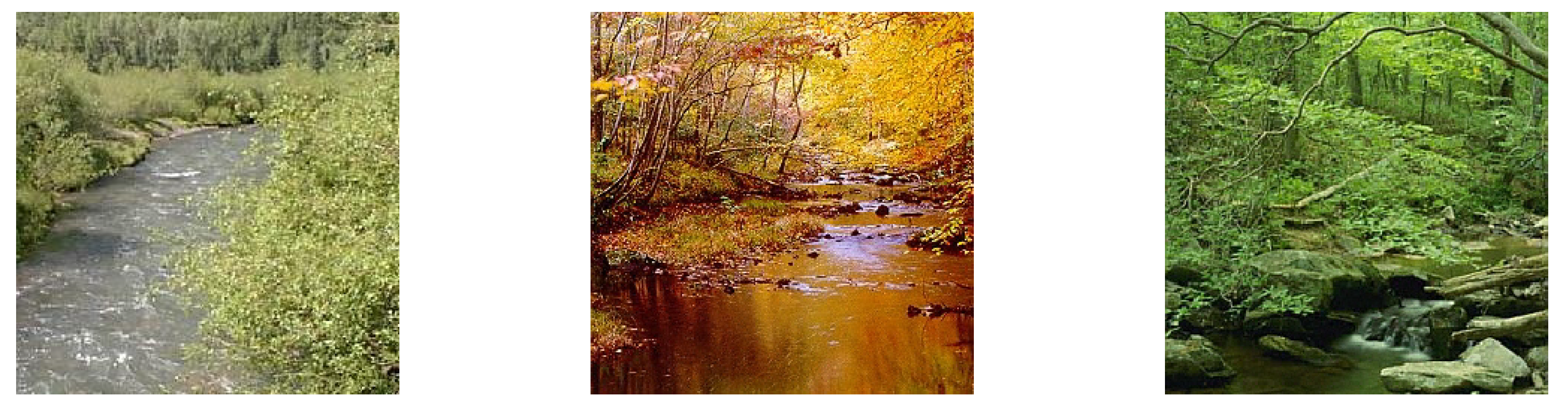
- Lacking Noise-Resilient Scene Classification Algorithm: since images’ categories are often annotated by human beings, and it is natural for us to make some incorrect annotations especially when we are provided with massive images. In addition, an image may cover several semantics. For example, the images in Figure 1 can be annotated with the scene of river or forest, but, under the framework of multi-classification, only one category is assigned to each of the images. Thus, noisy labels are often inevitable in scene classification. It is necessary to devise a scene classification algorithm that is robust to noisy labels.
- -
- Lacking Online Scene Classification Algorithm: a vast majority of existing scene classification algorithms predominantly focus on the static setting and require the accessibility of the whole image data set. However, with the constant improvement of satellite and aerospace technology, a large number of images are available continuously in the streaming fashion. The requirement to have all the training data in prior to training poses a serious constraint in the application of traditional scene classification algorithms based on batch learning techniques. To this end, it is necessary and of vital importance to perform online scene classification to adapt to the streaming data accordingly.
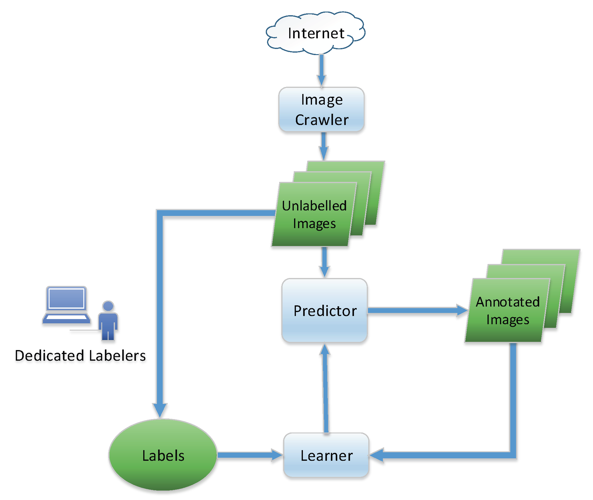
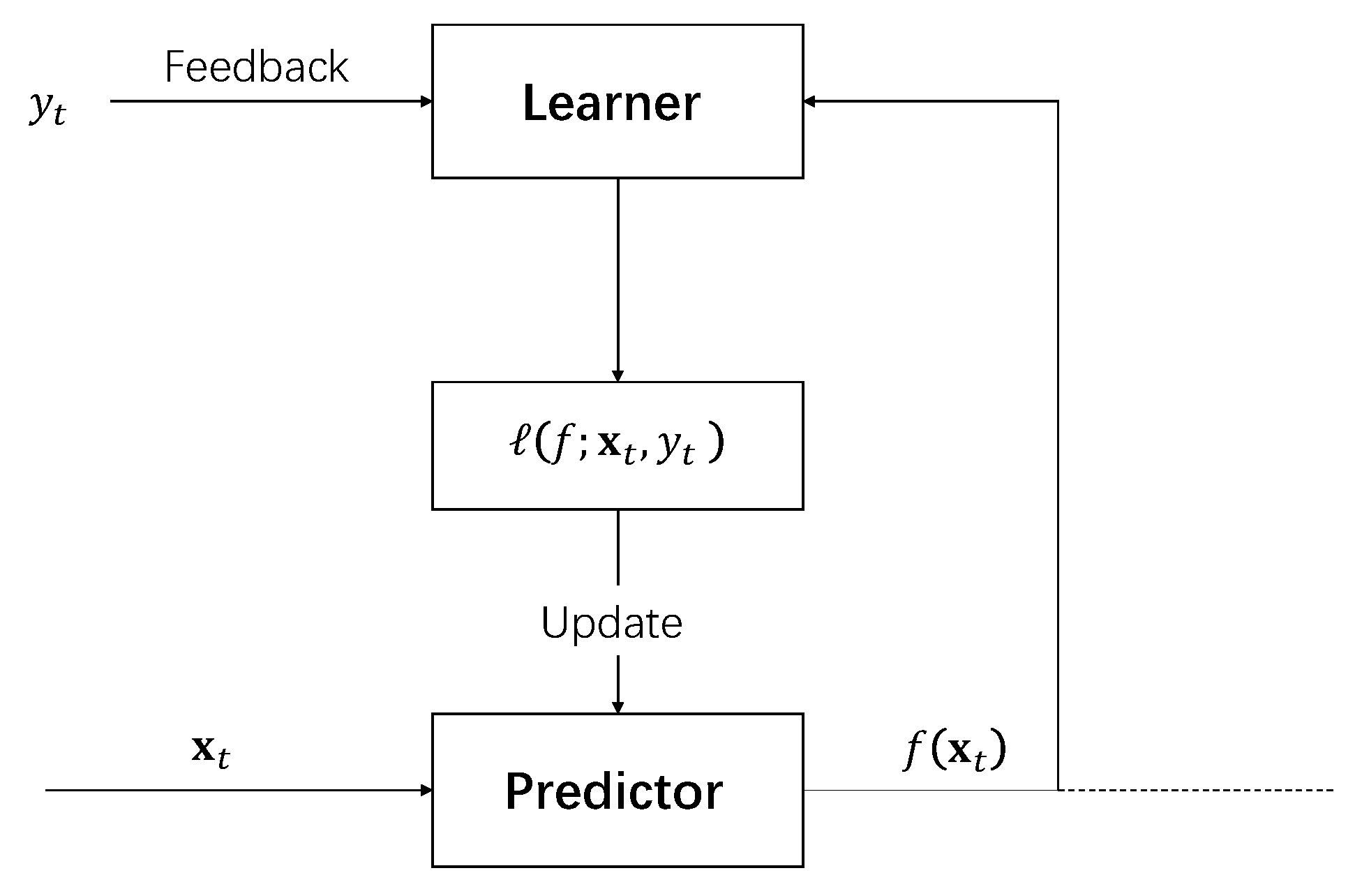
To tackle the above challenges, in this paper, we propose a noise-resilient online multi-classification algorithm to promote the scene classification problem for remote sensing images. Specifically, we generalize the ramp loss designed for a batch learning algorithm, e.g., ramp-Support Vector Machine (SVM), to the online learning setting and employ the Online Gradient Descent (OGD) algorithm to optimize the decision function in the Reproducing Kernel Hilbert Space. To effectively reduce the impact of noises, an adjust strategy to dynamically control the threshold parameter s in ramp loss is given in the proposed algorithm. Large-scale examples are assumed to arrive consecutively one by one without any initial pre-labeled training set for the initialization of classifier. In the online learning procedure, as shown in Figure 2, the parameters of the predictor (classifier) are updated in an iterative manner with sequential incorporated examples. The noise-resilient online multi-classification algorithm we proposed in this paper has two major merits:
- -
- Noise-Resilient: by the dynamical setting of threshold parameter s, the noise which would lead to a large loss (larger than the threshold parameter) would be identified and won’t be incorporated into the Support Vectors (SVs) set.
- -
- Sparsity: as can be seen from Figure 3, only a fraction of examples (with the loss between s and 1) would serve as Support Vectors (SVs). It is designed to reduce the computational cost and enjoy the perfect scalability property.
The remainder of the paper is organized as follows: Section 2 reviews related work along scene classification and online learning. Section 3 introduces the proposed noise-resilient online learning algorithm for scene classification. Section 4 presents experimental results with discussions. Section 5 concludes the whole paper.
2. Related Work
In this section, we review the related work from two aspects: scene classification and online learning.
Scene classification is a fundamental task in the remote sensing image analysis field. The core aim of scene classification is to identify the land-cover categories of remotely sensed image patches. Numerous feature learning algorithms have been presented for scene classification. In the earlier years, feature extraction algorithms including GIST (represents the dominant spatial structure of a scene by a set of perceptual dimensions based on the spatial envelope model) [17], BoVW (bag-of-visual-words) model [11] and VGGNet (based on deep convolutional neural network model) [18], focus on hand-crafted features. Recently, data-driven features are developed via unsupervised feature learning algorithms [1,12,19]. For example, Zhang et al. propose a saliency guided unsupervised feature learning approach that is named as an auto-encoder. Romero et al. introduce the highly efficient conforcing lifetime and population sparsity (EPLS) algorithm into the auto-encoder to improve the classification performance [19]. A multiple feature-based remote sensing image retrieval approach was proposed in [12] by combining hand-crated features and data-driven features via unsupervised feature learning. In addition, an incremental Bayesian approach has also been presented to address the problem in image processing to learn generative visual models from a few training examples [20].
Instead of training the classifier again from scratch on the combined training set, the online learning algorithm incrementally updates the classifier to incorporate new examples into the learning model [21]. In this way, online learning can significantly save on computation costs and be more suitable to deal with large scale problems. In recent years, online learning has been extensively studied in the machine learning community. For example, Song et al. propose an incremental online algorithm to dynamically update the LS-SVM model when a new chunk of samples are incorporated into the SV set [22]. Hu et al. use an incremental online variant of the nearest class mean classifier and update the class means incrementally [23]. A novel online universal classifier capable of performing the multi-classification problem is proposed in [24]. In order to solve the cost-sensitive classification task on the fly, some novel online learning algorithms are proposed [25] to directly optimize different cost-sensitive metrics.
3. Method
In this section, we propose a noise-resilient online learning algorithm for scene classification of remote sensing images. A vast majority of existing online classification algorithms are mainly designed to learn discriminant information from clean data. However, in the scenario of scene classification, labels of some images could be noisy and erroneous, mainly because of the imperfect human labeling process and the inherent attribute of multiple label (as shown in Figure 1). To enable the online classification on streaming remote sensing images and to alleviate the negative impacts from noisy labels, we generalize the ramp loss designed for batch learning algorithm, i.e., ramp-SVM, to the online learning setting. Next, we propose a novel strategy to dynamically adjust the ramp loss parameter s.
3.1. Ramp Loss
In the case of pattern recognition, one argument was that the misclassification rate is poorly approximated by convex losses such as the hinge loss or the least square loss. Researchers proposed non-convex alternatives, such as hard-margin loss, Laplace error penalty [26], normalized sigmoid loss [27], -learning loss [28], ramp loss [29], etc. Among the mentioned non-convex losses, ramp loss which also called truncated hinge loss [30] is an attractive one. The merits of ramp loss proposed by Collobert et al. lie in two folds, i.e., scalability and noise-resilient [29].
Steinwart shows that the number of SVs, i.e., n, increases in classical SVMs and its online version Pegasos linearly with the number of training examples N [31]. More specifically, where is the best possible error achievable in the chosen feature space . Since the SVM training and recognition times grow quickly with the number of SVs, it appears obviously that SVMs cannot deal with large scale data. The curse can be exorcised by replacing the classical hinge loss by a non-convex loss function, e.g., the ramp loss. Shown in Figure 3, replacing hinge loss by ramp loss guarantees that examples with score wont be selected as SVs. The increased sparsity leads to better scaling properties for ramp-SVMs. Using the ramp loss, Collobert et al. obtained the ramp loss support vector machine (ramp-SVM) [29].
In addition, in classification methodologies, robustness to noise is always an important issue. The effect of noise samples can be significantly large since the penalty given to the outliers by the hinge loss is quite huge. In fact, any convex loss is unbounded. In ramp loss, the loss of any example has an upper bound, so it can control the effect of noisy sample and remove the effect of noise. Plots of hinge loss and ramp loss in Figure 3 show the robustness (noise-resilient) of the ramp loss.
The sparsity and noise-resilient arguments provide the motivation for using ramp loss as the loss function, and using it as a base to develop an online learning algorithm for large scale scene classification problems.
3.2. Online Learning Algorithm
One of the most common and well-studied tasks in data mining and knowledge discovery is classification. Over the past decades, a great deal of research has been performed on inductive learning methods for classification such as decision trees, artificial neural networks, and support vector machines. All of these techniques have been successfully applied to a great number of real-world problems. However, their standard application requires the availability of all of the training data at once, making their use for large-scale data mining applications and mining task on streaming data problematic [32].
In recent years, a great deal of attention in the machine learning community has been directed toward online learning methods (shown in Figure 4) such as Forgetron [33], online Passive Aggressive algorithm [34], Projectron [35], bounded online gradient descent algorithm [36], and online soft-margin kernel learning algorithm [37], to name a few. However, these online learning algorithms are proposed based on clean data. On the other hand, there are comparably few studies on online learning from noisy examples, and, in particular, from noisy labels.
In this work, we investigate the extent to the scenario of examples with noise which are not uncommon in scene categorization. Based on kernel trick and ramp loss, a sparsity and noise-resilient multi-classification algorithm is proposed for scene categorization problem.
3.3. Noise-Resilient Online Multi-Classification Algorithm
In this subsection, we introduce a sparse and robust online learning algorithm to perform a scene classification task when images’ labels are noisy or even erroneous. Specifically, we first introduce the proposed online learning algorithm for binary classification problem, and then present the general formulation to tackle multi-classification problems.
For similarity, we begin with the binary classification problem. In this scenario, the goal is to learn a series of nonlinear mapping function : based on a sequence of examples , where t is the current time stamp, d stands for the number of features, denotes the feature vector of remote sensing image and is the scene category of an image. Suppose that images arrive continuously in a streaming fashion, and the online classification algorithm makes the prediction in a sequential way. Specifically, each time when an image arrives, we first apply feature representation algorithm, e.g., Vector of Locally Aggregated Descriptors (VLAD) [38], Visual Geometry Group Descriptors (VGG) [18], Scale Invariant Feature Transform (SIFT) [39], or Spatial Envelope Model (GIST) [17] to obtain its representation vector , and then predicts its label as by the latest decision function . After the true label is revealed, the algorithm suffers an instantaneous loss
with the specification of loss function as ramp loss. In addition, the online classification algorithm updates the classifier by incorporating the new sample for the next round. Here, we assume that the nonlinear mapping f belongs to a Reproducing Kernel Hilbert Space (RKHS) (Given a nonempty set and a Hilbert space of functions , is an RKHS [40] endowed with kernel function if k has the reproducing property:
in particular, , and k is called the reproducing kernel for ).
Similar to the standard SVMs, our algorithm tries to find the optimal decision function by optimizing the regularized loss function of examples , i.e.,
Note that Equation (2) is not a convex optimization problem, but it can be formulated as a Difference of Convex (DC) programming. The Concave-Convex Procedure (CCCP) [41] may be applied to get the optimal solution. However, it falls into the category of batch learning algorithms and cannot meet the real-time requirement when dealing with streaming data. In the current work, we employ the well known online gradient descent (OGD) [42] framework Equation (3) to find the near-optimal solution. It is a trade-off between the accuracy and scalability:
Here, stands for the Gâteaus derivative of ramp loss . We can deduce as the following:
Now, we extend the sparse and noise-resilient online classification algorithm to the case of the multi-classification problem. Assume that there is a sequence of examples , where is the feature representation of the ith image and is the corresponding label that belongs to a label set . Similar to the multi-class SVM formulation proposed by Crammer and Singer [43], the multi-class model is defined as:
where is the predictor associated with the kth class. Assume that is a c-dimensional vector with as its kth component, i.e., . Similar to the aforementioned binary classification problem, the multi-class online learning algorithm receives examples in a sequential order and updates continuously. In particular, when we receive the new image , our algorithm predicts the label according to Equation (6). After the prediction, our algorithm receives the true label . The instantaneous loss specified by the ramp loss in the case of multi-class scenario is defined as:
with the notation of . Given and , we list the update rule for decision function according to the deduced OGD framework Equation (5) as:
where . In the case of or , the instantaneous loss is constant, and the gradient is zero. Thus, we don’t update the decision function. Otherwise, if , we get the formula:
One should note that the update rule in the case of binary classification can also be formulated into the framework of multi-classification by the replacement of f by .
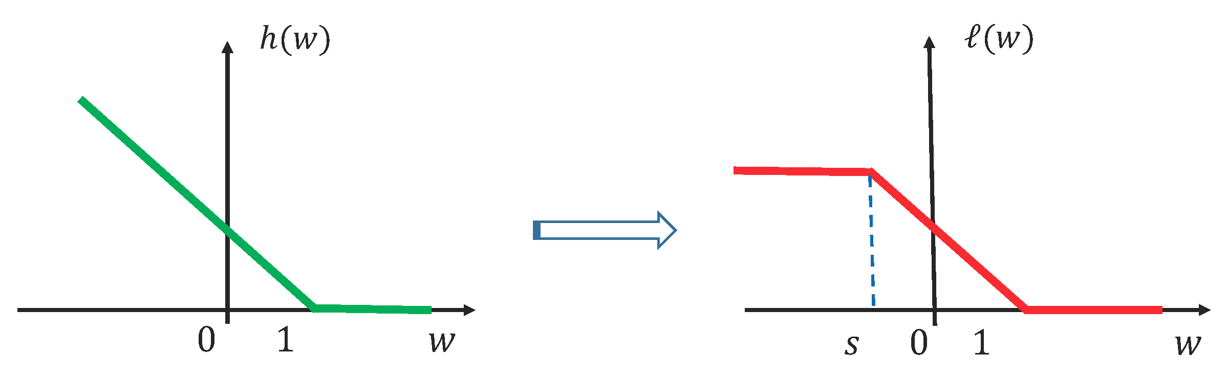
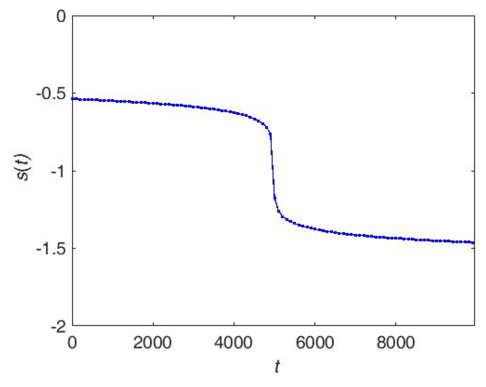
As shown in Equation (4), there is a noise-resilient parameter s ranging from in the proposed noise-resilient online learning algorithm. The smaller the parameter s, the closer the proposed algorithm is to the classical Pegasos algorithm proposed in [44]. Meanwhile, when the parameter is set as 1, the proposed algorithm won’t learn from any example and never update the classifier. It is an urgent issue to give a parameter setting strategy to assist the proposed noise-resilient algorithm with adjusting the ramp loss parameter s adaptively. In the current work, we set the parameter as Equation (11) and show it in Figure 5. In Equation (11), c stands for the number of categories and n is an estimate number of examples:
We summarize the proposed noise-resilient online multi-classification algorithm (Algorithm 1) as follows.
| Algorithm 1 Noise-Resilient Online Multi-classification Algorithm |
|
4. Experiments
In this section, we conduct experiments to evaluate the performance of the proposed noise-resilient online multi-classification algorithm. All experiments are performed in a MATLAB 7.14 environment on a PC with 3.4 GHz Intel Core i5 processors and 8G RAM running under the Windows 10 operating system. The source code of the proposed algorithm will be available upon the acceptance of the manuscript. First, we perform the parameter sensitivity study to show how the ramp loss parameter s affects the classification results. Then, we present an experiment on synthetic data sets to show the efficacy and efficiency of the proposed method for noisy labels. Finally, we conduct extensive experiments to evaluate the performance of the proposed algorithm on different remote sensing image classification tasks.
4.1. Parameter Sensitivity Study
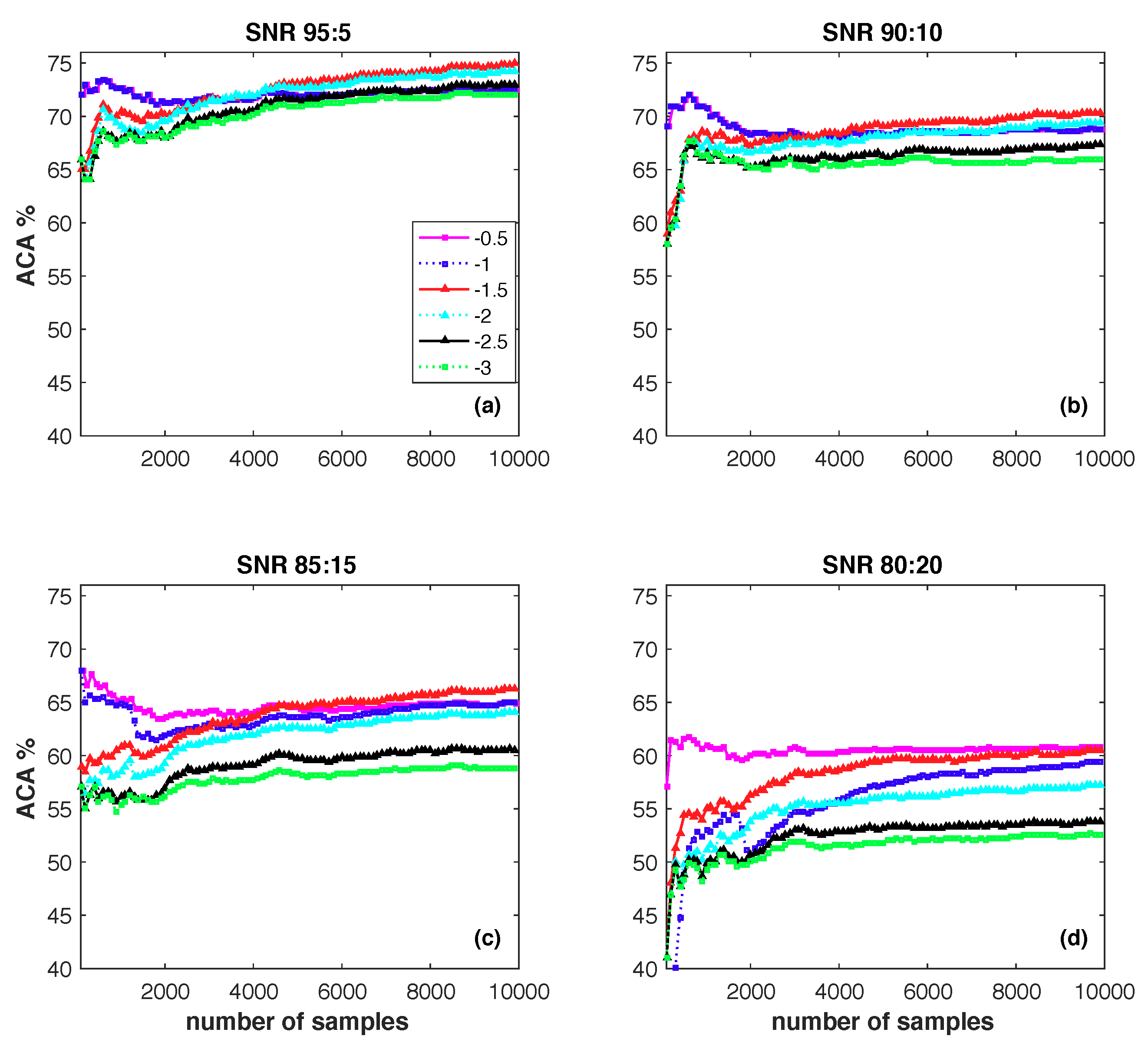
There is an important hyper parameter in the proposed online classification algorithm: ramp loss parameter s. The parameter s controls the sparsity and noise-resilient level of the proposed model. The bigger the parameter s, the sparser the proposed algorithm is, and the less noisy examples will be incorporated into the learning model. However, bigger parameter s will decrease more informative examples and further influence the classification efficacy. To study how this parameter affects the classification result, we conduct an experiment on synthetic data sets. Specifically, we derive a set of synthetic data sets from a real-world data set, i.e., Adult (http://archive.ics.uci.edu/ml/datasets/Adult), which consists of 7579 negative samples and 2372 positive samples, by adding some random noise to the labels. To simulate the case of noisy labels, we randomly change some entries in the label vector . The percentage of changed labels is varied among {5%, 10%, 15%, 20%}. In this way, we generate synthetic data sets with signal-to-noise ratio (SNR) as 95:5, 90:10, 85:15, 80:20, respectively. In this study, we tune the parameter s from {} and draw a 2D performance variation (Average Classification Accuracy, ACA %) figure w.r.t. the different parameter setting of s in Figure 6.
We make the following observations from Figure 6:
- -
- At the beginning of the online learning process, the bigger s always outperforms small ones.
- -
- On the whole, the higher the noise level is, the worse the performance of the algorithm will be. On a fixed noise level, e.g., SNR 90:10, a smaller s will incorporate more SVs into the classifier. Among them some are useful examples and the other are noisy examples. Thus, a proper setting for s is the key problem for the proposed noise-resilient online classification algorithm.
- -
- The proposed algorithm is sensitive to ramp loss parameter s. In this study, gives the overall best performance, and is the worst one. Any fixed setting of s can not outperform others in all four of the situations.
Regarding this, we propose an adaptive parameter setting strategy in Equation (11) to adjust s dynamically and investigate its performance in the next subsection.
4.2. Synthesis Data Sets
We investigate the proposed noise-resilient online classification algorithm on synthetic data sets when label information is noisy. Specifically, we attempt to answer the following two questions:
- -
- Sparsity: How sparse is the proposed online classification algorithm for streaming data?
- -
- Noise-Resilient: How effective is the proposed online classification algorithm for data with noisy labels?
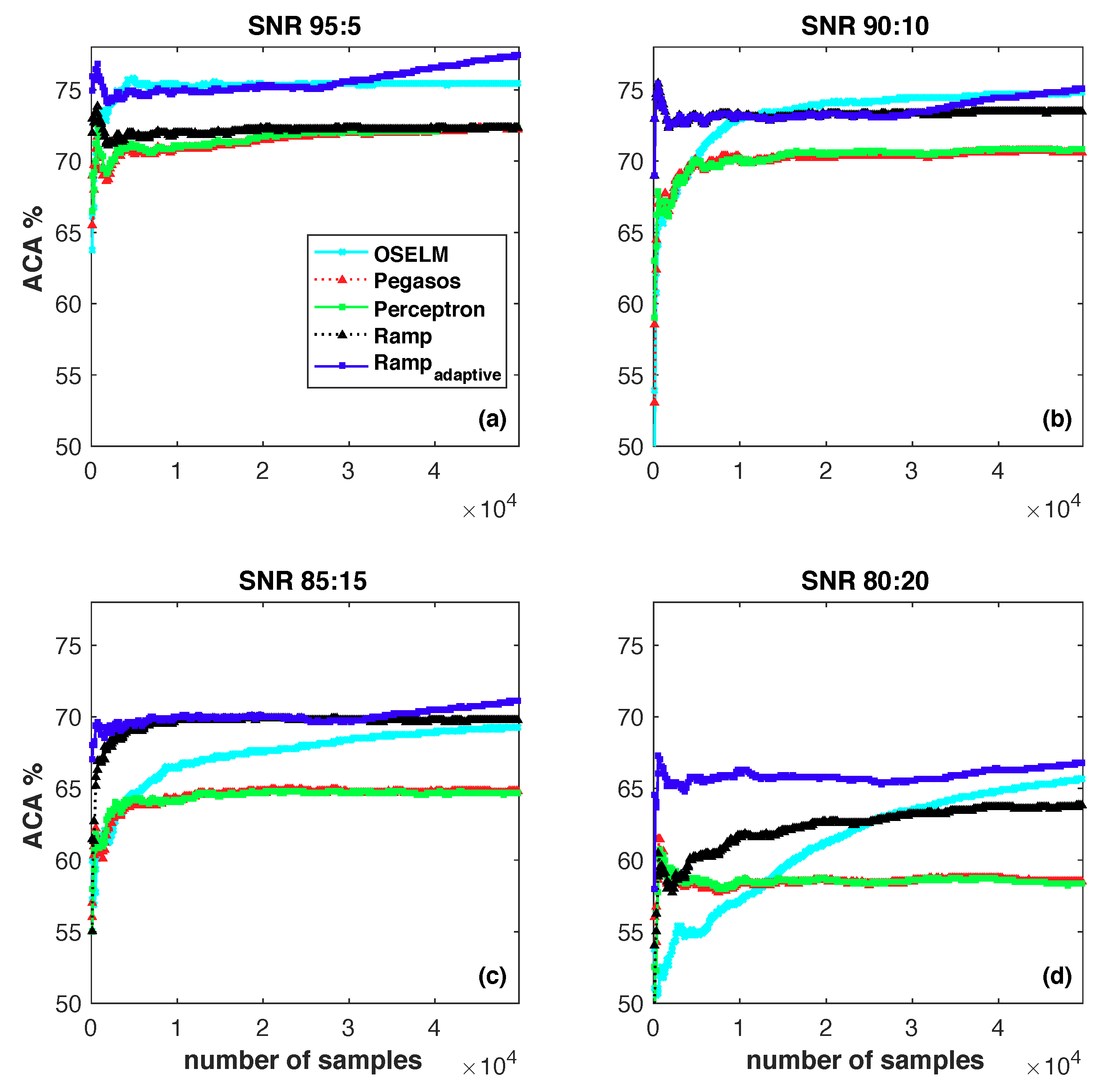
Our algorithm incorporated with adaptive parameter s is denoted as ; meanwhile, the algorithm with fixed parameter settings is denoted as Ramp. We compare the proposed and Ramp with the following widely used online learning algorithms:
For OSELM, we specify the sigmoid function as the active function and set the number of hidden neurons as 50. We use the default setting for parameters in Pegasos and Perceptron: the regularization parameter is set as for Pegasos and the learning rate parameter is set as 1 for Perceptron. In Ramp, the parameter s is set to be . In the current experiments, the RBF kernel is selected as the kernel function for kernel based learning algorithms. Kernel parameter is set as , where d is the number of features. To simulate a large scale scenario, in the current experiment, we repeat the data of Adults five times. In addition, we randomly change some entries in the label vector with the percentage of {5%, 10%, 15%, 20%}. The classification performances of different algorithms are listed in Figure 7.
Figure 7a,b show that the average classification performance of is comparable to OSELM, and they outperform other algorithms. In Figure 7c,d, outperforms the other algorithms. It indicates that is indeed a noise-resilient algorithm that is able to mine discriminative information when the labels contain explicit noise.
To further investigate the superiority of the proposed algorithm on sparsity and efficiency, we compare the number of SVs and speedup rate of the proposed online learning algorithm w.r.t. the state-of-art online learning algorithms, i.e., Pegasos and Perceptron. One should note that the OSELM incrementally incorporates examples to update the learning model. As all of the learning examples serve as the SVs, the OSELM does not belong to the family of sparse learning algorithm. Thus, we did not investigate its sparsity and efficiency here. In Table 1, we show the number of support vectors (SVs) and running time that each method needs to perform online classification. Among the two proposed noise-resilient online classification algorithms, uses less SVs than Ramp and only costs half of the running time of Ramp on the four data sets. The proposed achieves about 2.7×, 3.3×, 3.8×, and 5.7× sparsity in the case of SNR 95:5, SNR 90:10, SNR 85:15 and SNR 80:20, respectively. As for running time, achieves about 3.5×, 5.2×, 5.8×, and 7.5× speedup in the case of SNR 95:5, SNR 90:10, SNR 85:15 and SNR 80:20, respectively. In a nutshell, the proposed online classification algorithm is more suitable to scale up among the online kernel learning algorithms.
4.3. Benchmark Data Sets
In this section, we will conduct extensive experiments to evaluate the performance of the proposed algorithm on different remote sensing image analysis tasks, including Outdoor Scene categories data set (http://people.csail.mit.edu/torralba/code/spatialenvelope/), UC Merced Landuse data set (http://weegee.vision.ucmerced.edu/datasets/landuse.html), and Aerial Image Data (AID) set (www.lmars.whu.edu.cn/xia/AID-project.html).
- -
- AID7 data set: AID is a large-scale aerial image data set, by collecting sample images from Google Earth imagery. AID7 is made up of the following seven aerial scene types: grass, field, industry, river lake, forest, resident, and parking. The AID7 data set has a number of 2800 images within seven classes and each class contains 400 samples of size 600×600 pixels.
- -
- Outdoor Scene categories data set: this data set contains eight outdoor scene categories, i.e., coast, mountain, forest, open country, street, inside city, tall buildings and highways. There are 2600 color images of 256×256 pixels. All of the objects and regions in this data set have been fully labeled. There are more than 29,000 objects.
- -
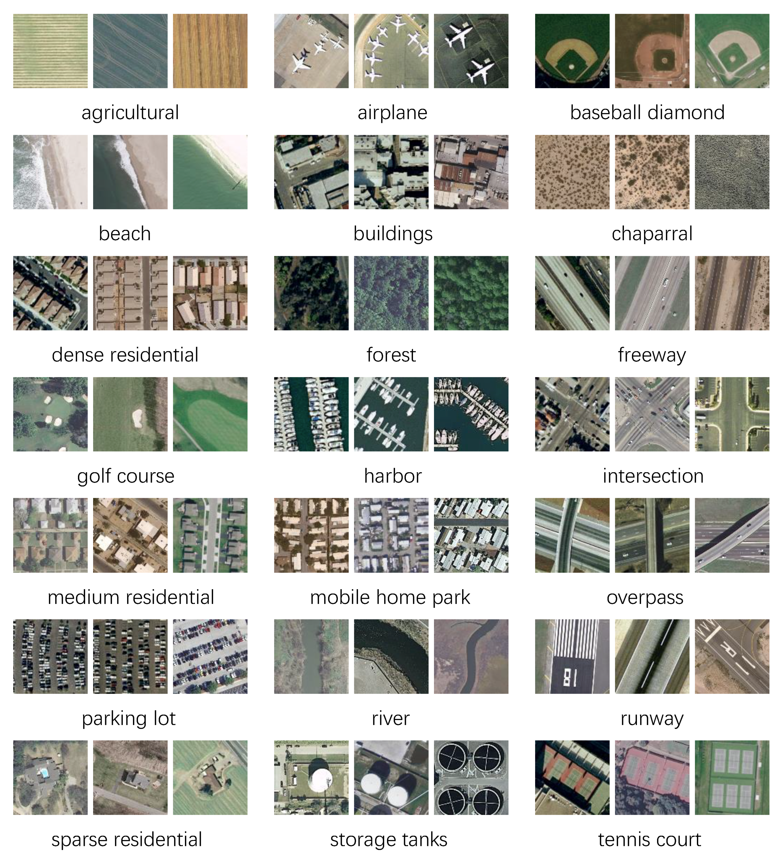
- UC Merced Landuse data set: the images in the UC Merced Landuse data set were manually extracted from large images from the USGS (United States Geological Survey) National Map Urban Area Imagery collection for various urban areas around the country. The pixel resolution of this public domain imagery is one foot. The UC Merced data set contains 2100 images in total and each image measures 256×256 pixels. There are 100 images for each of the following 21 classes: agricultural, airplane, baseball diamond, beach, buildings, chaparral, dense residential, forest, freeway, golf course, harbor, intersection, medium residential, mobile home park, overpass, parking lot, river, runway, sparse residential, storage tanks, and tennis court. Some sample images from this data set are shown in Figure 8.
- -
- AID30 data set: similar to the AID7 data set, this data set is made up of the following 30 aerial scene types: airport, bareland, baseballfield, beach, bridge, center, church, commercial, dense residential, desert, farmland, forest, industrial, meadow, medium residential, mountain, park, parking, playground, pond, port, railway station, resort, river, school, sparse residential, square, stadium, storage tanks and viaduct. In total, the AID30 data set has a number of 10,000 images within 30 classes and each class contains about 200 to 400 samples of size 600×600 pixels.
In this experiment, we randomly select 50% of the images from each class to form the training set and the remaining 50% images are used for testing. This procedure is repeated five times and the average performance is finally reported. We use the GIST Descriptor (http://people.csail.mit.edu/torralba/code/spatialenvelope/) to transform an image into a feature vector of 512 dimensions. For OSELM, we conduct comparison experiments on dataset AID7 and Outdoor Scene to check if different settings for OSELM can change the results significantly. We specify the activation function to be sigmoid, sin, rbf, and hardlim, respectively. Meanwhile, set the number of hidden nodes as 50, 100, 200, and 300, respectively. Comparison experiments show that the sigmoid function with the number of hidden neurons as 200 is a good candidate for OSELM without prior knowledge. Without loss of generality, we specify the sigmoid function as active function and set the number of hidden neurons as 200. For kernel based learning algorithms, polynomial kernel is selected as the kernel function for it is extensively used for image processing. Here, we set to be , where d is the number of features, to be 0 and polynomial order p to be 1.
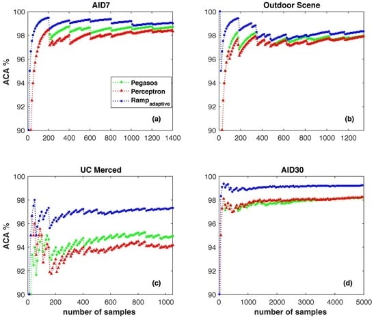
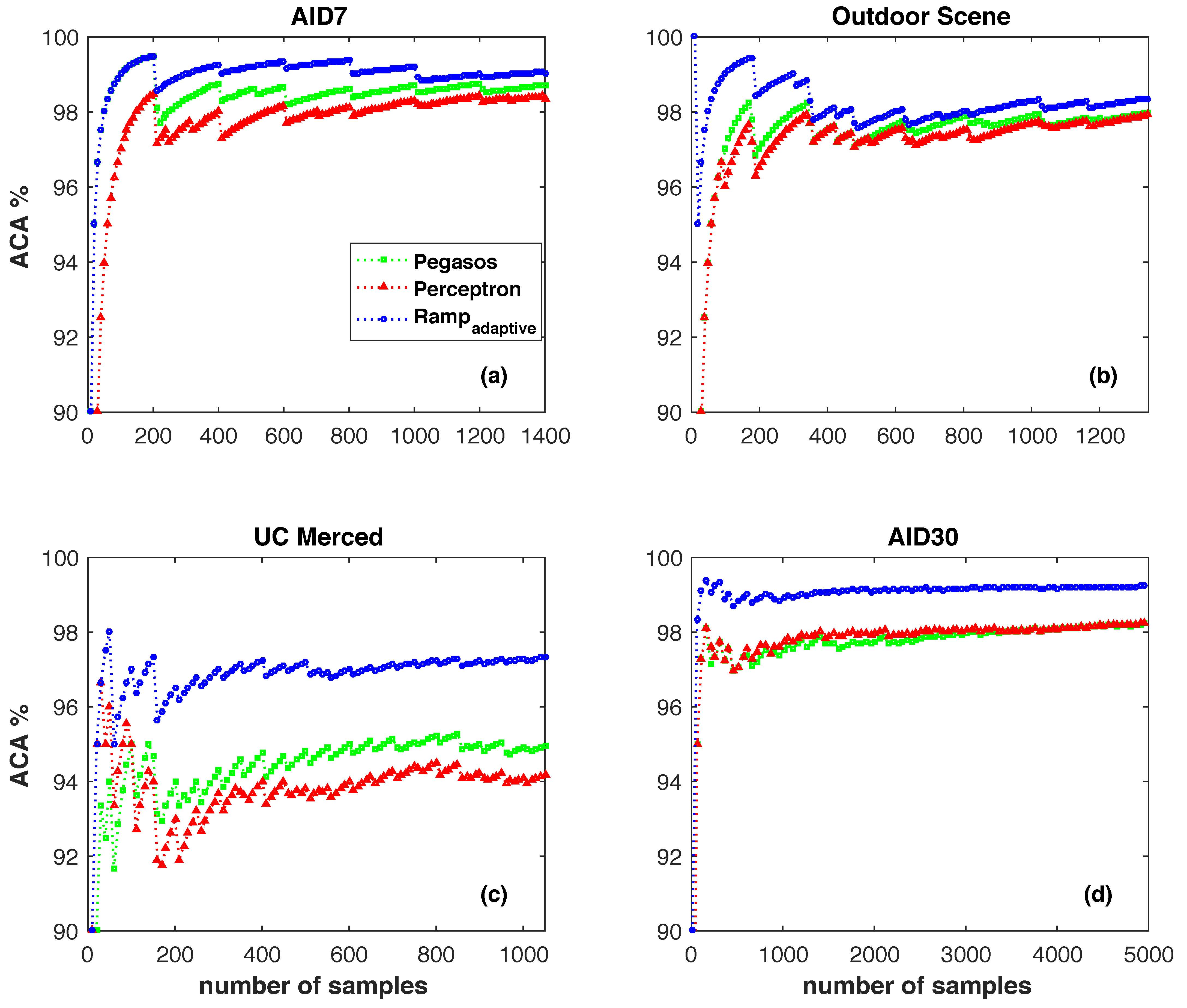
First of all, we show the behavior of the algorithms over time. Figure 9 shows the average online classification accuracy. The average online classification accuracy is the total number of correctly classified samples seen as a function of the number of all samples. From Figure 9, we can draw the following conclusions: (1) kernel based online learning algorithms consistently outperform the OSELM, which validates that polynomial kernel is a good candidate for the image classification problem; (2) always beats other kernel based online learning algorithms, i.e., Pegasos and Perceptron; (3) in Figure 9c, the proposed clearly shows a big advantage over the state-of-the art online learning methods.
For a comprehensive comparison, Table 2 summarizes the frequently used criteria: Overall Accuracy (%), Average Accuracy (%), Kappa and running time of different online learning algorithms. It can be observed from Table 2 that kernel based online learning algorithms significantly improve the performance (Overall Accuracy (%), Average Accuracy (%) and Kappa) compared with OSELM. The three kernel based online learning algorithms achieve similar performance and the proposed slightly outperforms others in four data sets. The column of Time (s) shows that OSELM is extremely efficient. The proposed costs significantly more running time on small scale data sets AID7, Outdoor Scene, and UC Merced (around 1000 testing samples), which conflicts with the observation in Table 1. The reason lies in the extra computation of the ramp loss parameter s in Equation (11) per iteration in . On small scale data sets, the number of SVs in different online learning algorithms is comparable and so is the iteration number. In this case, the proposed costs more running time than Pegasos and Perceptron. As time goes by, more and more learning samples will be misclassified. All of the misclassified samples are selected as SVs and will further be used to update the learning model of Pegasos and Perceptron. In contrast, only a small fraction of misclassified samples will be selected as SVs for the model updating of . Thus, the efficiency and sparsity advantages of will be fully demonstrated when dealing with large-scale problems.
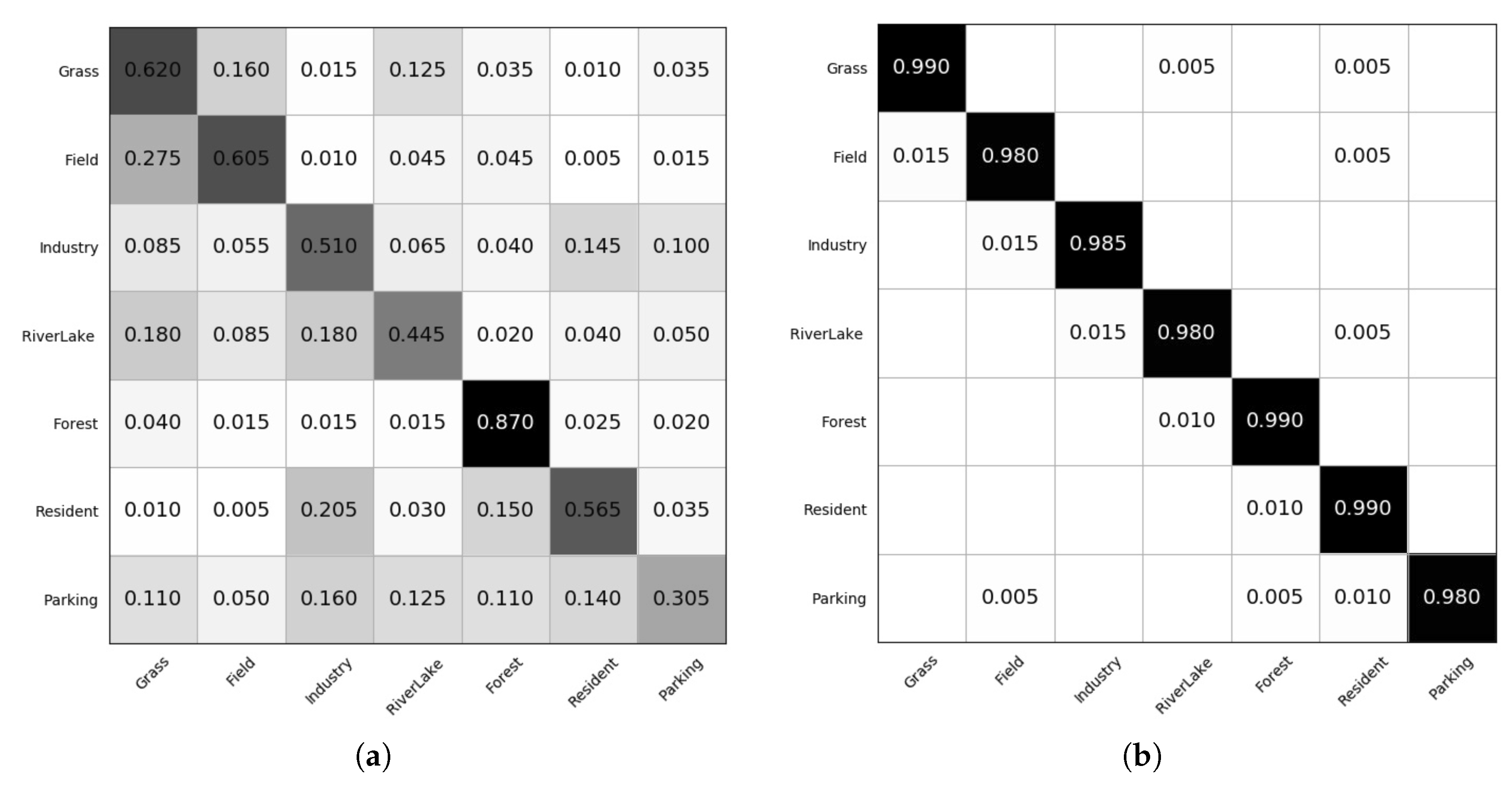
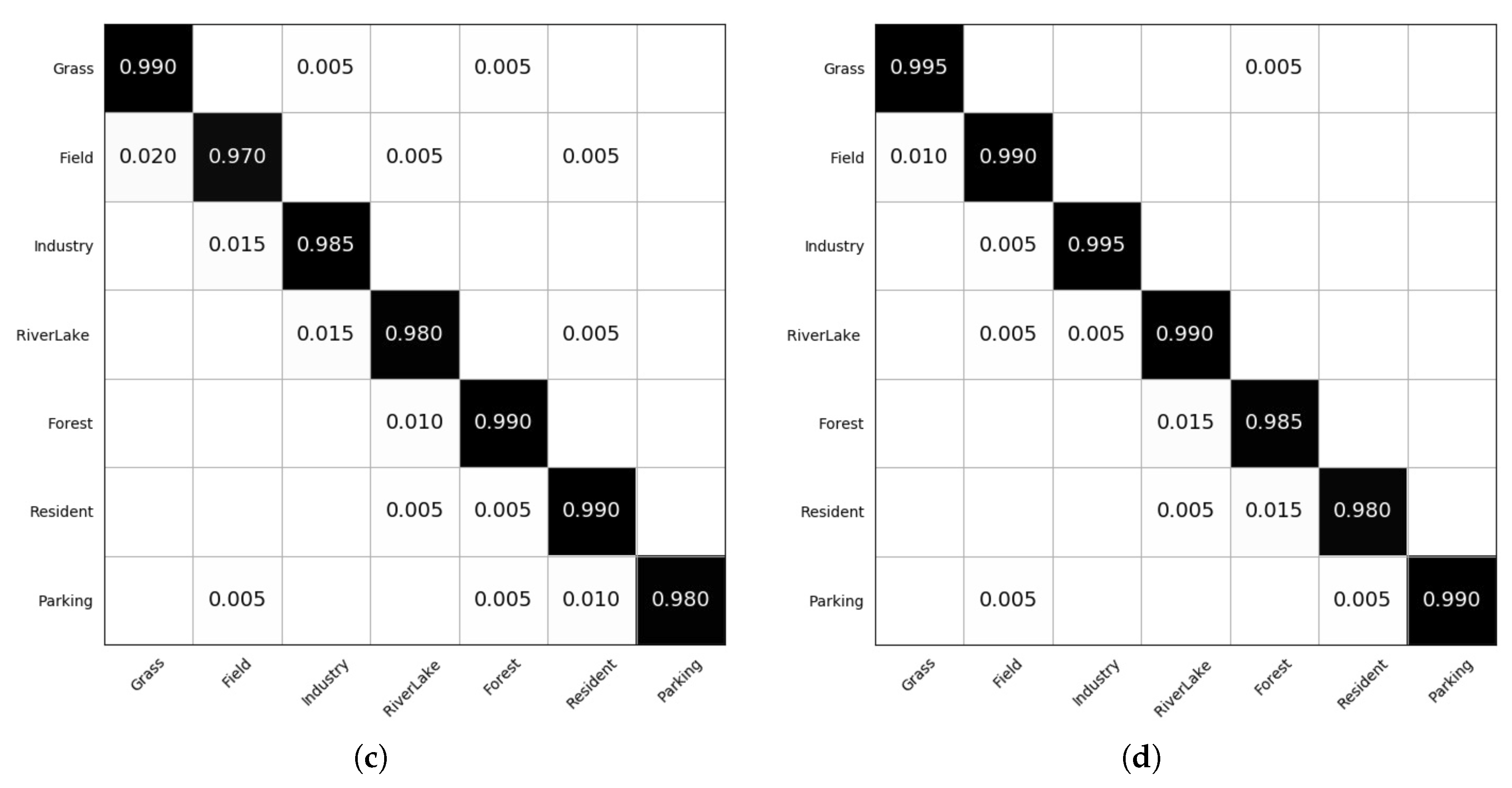
Figure 10 shows the confusion matrix of online learning algorithms OSELM, Pegasos, Perceptron and the proposed on the AID7 data set. From the figure, we observe that accuracies above 97% are obtained for all seven of the classes with kernel based online learning approaches. As for the three kernel based online learning algorithms, our proposed outperforms Pegasos and Perceptron on the classes “Grass”, “Field”, “Industry”, “RiverLake”, “Parking” and ’s performance is slightly lower than Pegasos and Perceptron upon “Forest” and “Resident”.
5. Conclusions
For a variety of reasons such as multiple label, human errors, etc., noisy labels are inevitable in the scenario of large scale scene classification problems. In this paper, we studied a novel problem on performing online scene classification of remote sensing images and providing a noise-resilient online classification algorithm to incrementally predict the scene category of new images. Due to the fact that less examples are incorporated into the SV set during the learning procedure, the proposed method leads to better sparsity and hence much faster learning speed. The aforementioned merits make it a good candidate for large scale scene classification of remote sensing images. We conduct extensive experiments on both synthetic and real-world data sets to validate the efficiency and efficacy of the proposed algorithm. Though experimental studies shows the potential of the proposed online learning algorithm, relevant theoretical analysis has not been carried out deeply and will be our future investigation focus. In addition, with the increasing number of SVs, the computational efficiency of updating the learning model will decrease gradually. Incorporating the budget strategy can further improve the efficiency of the proposed online learning algorithm and will be another focus of our investigation.
Author Contributions
L.J. and S.L. designed the algorithm; L.J. and P.R. wrote the draft manuscript; F.G. and Y.S. performed the experiments; S.L. revised the paper.
Funding
This research was funded by National Natural Science Foundation of China under Grant Nos. 61873279 and 61563018, the National Key Research and Development Program of Shandong Province under Grant No. 2018GSF120020 and Fundamental Research Funds for the Central Universities under Grant No. 16CX02048A.
Conflicts of Interest
The authors declare no conflict of interest.
References
- Zhang, F.; Du, B.; Zhang, L. Saliency-guided unsupervised feature learning for scene classification. IEEE Trans. Geosci. Remote Sens. 2015, 53, 2175–2184. [Google Scholar] [CrossRef]
- Yu, Y.; Liu, F. Dense connectivity based two-stream deep feature fusion framework for aerial scene classification. Remote Sens. 2018, 10, 1158. [Google Scholar] [CrossRef]
- Faisal, A.; Kafy, A.; Roy, S. Integration of remote sensing and GIS techniques for flood monitoring and damage assessment: A case study of naogaon district. Egypt. J. Remote Sens. Space Sci. 2018, 7, 2. [Google Scholar] [CrossRef]
- Bi, S.; Lin, X.; Wu, Z.; Yang, S. Development technology of principle prototype of high-resolution quantum remote sensing imaging. In Quantum Sensing and Nano Electronics and Photonics XV; International Society for Optics and Photonics: Bellingham, WA, USA, 2018. [Google Scholar]
- Weng, Q.; Quattrochi, D.; Gamba, P.E. Urban Remote Sensing; CRC Press: Boca Raton, FL, USA, 2018. [Google Scholar]
- Mukherjee, A.B.; Krishna, A.P.; Patel, N. Application of remote sensing technology, GIS and AHP-TOPSIS model to quantify urban landscape vulnerability to land use transformation. In Information and Communication Technology for Sustainable Development; Springer: Singapore, 2018. [Google Scholar]
- Li, P.; Ren, P.; Zhang, X. Region-wise deep feature representation for remote sensing images. Remote Sens. 2018, 10, 871. [Google Scholar] [CrossRef]
- Xia, G.S.; Hu, J.; Hu, F. AID: A benchmark data set for performance evaluation of aerial scene classification. IEEE Trans. Geosci. Remote Sens. 2017, 55, 3965–3981. [Google Scholar] [CrossRef]
- Aptoula, E. Remote sensing image retrieval with global morphological texture descriptors. IEEE Trans. Geosci. Remote Sens. 2014, 52, 3023–3034. [Google Scholar] [CrossRef]
- Yang, Y.; Newsam, S. Geographic image retrieval using local invariant features. IEEE Trans. Geosci. Remote Sens. 2013, 52, 818–832. [Google Scholar] [CrossRef]
- Yang, Y.; Newsam, S. Bag-of-visual-words and spatial extensions for land-use classification. In Proceedings of the 18th SIGSPATIAL International Conference on Advances in Geographic Information Systems, San Jose, CA, USA, 2–5 November 2010; pp. 270–279. [Google Scholar]
- Li, Y.; Zhang, Y.; Tao, C. Content-based high-resolution remote sensing image retrieval via unsupervised feature learning and collaborative affinity metric fusion. Remote Sens. 2016, 8, 709. [Google Scholar] [CrossRef]
- Yu, Y.; Gong, Z.; Wang, C. An unsupervised convolutional feature fusion network for deep representation of remote sensing images. IEEE Geosci. Remote Sens. Lett. 2018, 15, 23–27. [Google Scholar] [CrossRef]
- Wang, Q.; Liu, S.; Chanussot, J.; Li, X. Scene classification with recurrent attention of VHR remote sensing images. IEEE Trans. Geosci. Remote Sens. 2018. [Google Scholar] [CrossRef]
- Ma, X.; Liu, W.; Li, S.; Tao, D.; Zhou, Y. Hypergraph-Laplacian regularization for remotely sensed image recognition. IEEE Trans. Geosci. Remote Sens. 2018. [Google Scholar] [CrossRef]
- Wang, Q.; He, X.; Li, X. Locality and structure regularized low rank representation for hyperspectral image classification. IEEE Trans. Geosci. Remote Sens. 2018. [Google Scholar] [CrossRef]
- Oliva, A.; Torralba, A. Modeling the shape of the scene: A holistic representation of the spatial envelope. Int. J. Comput. Vis. 2001, 42, 145–175. [Google Scholar] [CrossRef]
- Simonyan, K.; Zisserman, A. Very deep convolutional networks for large-scale image recognition. arXiv 2014, arXiv:1409.1556. [Google Scholar]
- Romero, A.; Gatta, C.; Camps-Valls, G. Unsupervised deep feature extraction for remote sensing image classification. IEEE Trans. Geosci. Remote Sens. 2016, 54, 1349–1362. [Google Scholar] [CrossRef]
- Li, F.F.; Fergus, R.; Perona, P. Learning generative visual models from few training examples: An incremental Bayesian approach tested on 101 object categories. In Proceedings of the Conference on Computer Vision and Pattern Recognition Workshop, Washington, DC, USA, 27 June–2 July 2004; Volume 106, p. 178. [Google Scholar]
- Jian, L.; Shen, S.Q.; Li, J.D.; Liang, X.J.; Li, L. Budget online learning algorithm for least squares SVM. IEEE Trans. Neural Netw. Learn. Syst. 2017, 28, 2076–2087. [Google Scholar] [CrossRef] [PubMed]
- Song, X.X.; Jian, L.; Song, Y.Q. A chunk updating LS-SVMs based on block Gaussian elimination method. Appl. Soft Comput. 2017, 51, 96–104. [Google Scholar] [CrossRef]
- Hu, J.; Sun, Z.; Li, B. Online user modeling for interactive streaming image classification. In Proceedings of the Conference on Multimedia Modeling, Reykjavik, Iceland, 4–6 January 2017; pp. 293–305. [Google Scholar]
- Meng, J.E.; Venkatesan, R.; Ning, W. An online universal classifier for binary, multi-class and multi-label classification. In Proceedings of the IEEE International Conference on Systems, Man, and Cybernetics, Budapest, Hungary, 9–12 October 2017; pp. 3701–3706. [Google Scholar]
- Zhao, P.; Hoi, S.C.H. Cost-sensitive online active learning with application to malicious URL detection. In Proceedings of the ACM SIGKDD International Conference on Knowledge Discovery and Data Mining, Chicago, IL, USA, 11–14 August 2013; pp. 919–927. [Google Scholar]
- Jian, L.; Ma, X.; Song, Y.; Luo, S. Laplace error penalty-based M-type model detection for a class of high dimensional semiparametric models. J. Comput. Appl. Math. 2019, 347, 210–221. [Google Scholar] [CrossRef]
- Mason, L.; Bartlett, P.L.; Baxter, J. Improved generalization through explicit optimization of margins. Mach. Learn. 2000, 38, 243–255. [Google Scholar] [CrossRef]
- Shen, X.T.; Tseng. On ψ-learning. J. Am. Stat. Assoc. 2003, 98, 724–734. [Google Scholar] [CrossRef]
- Collobert, R.; Sinz, F.; Weston, J.; Bottou, L. Trading convexity for scalability. In Proceedings of the ACM International Conference on Machine Learning, Pittsburgh, PA, USA, 25–29 June 2006; pp. 201–208. [Google Scholar]
- Wu, Y.; Liu, Y. Robust truncated hinge loss support vector machines. Publ. Am. Stat. Assoc. 2007, 102, 974–983. [Google Scholar] [CrossRef]
- Steinwart, I. Sparseness of support vector machines. J. Mach. Learn. Res. 2008, 4, 1071–1105. [Google Scholar]
- Aggarwal, C.C. Data Mining: The Textbook; Springer: Berlin, Germany, 2015. [Google Scholar]
- Dekel, O.; Shalev-Shwartz, S.; Singer, Y. The Forgetron: A kernel-based Perceptron on a budget. SIAM J. Comput. 2008, 37, 1342–1372. [Google Scholar] [CrossRef]
- Crammer, K.; Dekel, O.; Keshet, J. Online passive-aggressive algorithms. J. Mach. Learn. Res. 2006, 7, 551–585. [Google Scholar]
- Francesco, O.; Joseph, K.; Barbara, C. The projectron: A bounded kernel-based Perceptron. In Proceedings of the International Conference on Machine Learning, Helsinki, Finland, 5–9 July 2008; pp. 720–727. [Google Scholar]
- Zhao, P.; Wang, J.; Wu, P. Fast bounded online gradient descent algorithms for scalable kernel-based online learning. In Proceedings of the International Conference on Machine Learning, Edinburgh, UK, 26 June–1 July 2012; pp. 169–176. [Google Scholar]
- Jian, L.; Li, J.D.; Liu, H. Toward online node classification on streaming networks. Data Min. Knowl. Discov. 2018, 32, 231–257. [Google Scholar] [CrossRef]
- Jégou, H.; Douze, M.; Schmid, C.; Pérez, P. Aggregating local descriptors into a compact image representation. In Proceedings of the Computer Vision and Pattern Recognition, San Francisco, CA, USA, 13–18 June 2010; pp. 3304–3311. [Google Scholar]
- Cheung, W.; Hamarneh, G. n-SIFT: n-dimensional scale invariant feature transform. IEEE Trans. Image Process. 2009, 18, 2012–2021. [Google Scholar] [CrossRef] [PubMed]
- Schölkopf, B.; Smola, A.J.; Bach, F. Learning with Kernels: Support Vector Machines, Regularization, Optimization, and Beyond; MIT Press: Cambridge, UK, 2002. [Google Scholar]
- Yuille, A.L.; Anand, R. The concave-convex procedure. Neural Comput. 2003, 15, 915–936. [Google Scholar] [CrossRef] [PubMed]
- Shalev-Shwartz, S. Online learning and online convex optimization. Found. Trends Mach. Learn. 2012, 4, 107–194. [Google Scholar] [CrossRef]
- Crammer, K.; Singer, Y. On the algorithmic implementation of multiclass kernel-based vector machines. J. Mach. Learn. Res. 2002, 2, 265–292. [Google Scholar]
- Shalev-Shwartz, S.; Singer, Y.; Srebro, N.; Cotter, A. Pegasos: Primal estimated sub-gradient solver for SVM. Math. Program. 2011, 127, 3–30. [Google Scholar] [CrossRef]
- Huang, G.; Zhou, H.; Ding, X.; Zhang, R. Extreme learning machine for regression and multiclass classification. IEEE Trans. Syst. Man Cybern. Part B Cybern. 2012, 42, 513–529. [Google Scholar] [CrossRef] [PubMed]
- Liang, N.; Huang, G.; Saratchandran, P.; Sundararajan, N. A fast and accurate online sequential learning algorithm for feedforward networks. IEEE Trans. Neural Netw. 2006, 17, 1411–1423. [Google Scholar] [CrossRef] [PubMed]
- Crammer, K.; Singer, Y. Ultraconservative online algorithms for multiclass problems. J. Mach. Learn. Res. 2003, 3, 951–991. [Google Scholar]
Figure 1.
Image may be associated with more than one semantic category. Three images listed here can be annotated with the scene of rivers or forests.
Figure 1.
Image may be associated with more than one semantic category. Three images listed here can be annotated with the scene of rivers or forests.

Figure 2.
Illustration of the online scene classification framework. As time goes by, unlabeled images are assumed to arrive consecutively. A predictor is applied to annotate the images that have arrived. When the true label is revealed, the online learner updates the predictor for the next prediction.

Figure 3.
Hinge loss is shown in the first panel and the second panel lists the ramp loss.

Figure 4.
An illustration schematic of the online learning algorithm. Online learning is performed in a sequence of consecutive rounds. At each round t, the online learner picks a predictor f to make the prediction . When the true label is revealed, the online learner suffers from an instantaneous loss and updates the predictor for the next prediction.

Figure 5.
An illustration of the adaptive parameter setting for s.

Figure 6.
Average classification accuracy with respect to the parameter s on different synthetic data sets: (a) SNR 95:5; (b) SNR 90:10; (c) SNR 85:15 and (d) SNR 80:20.
Figure 6.
Average classification accuracy with respect to the parameter s on different synthetic data sets: (a) SNR 95:5; (b) SNR 90:10; (c) SNR 85:15 and (d) SNR 80:20.

Figure 7.
Comparison of online learning algorithms w.r.t. average classification accuracy on synthetic data sets: (a) SNR 95:5; (b) SNR 90:10; (c) SNR 85:15 and (d) SNR 80:20.
Figure 7.
Comparison of online learning algorithms w.r.t. average classification accuracy on synthetic data sets: (a) SNR 95:5; (b) SNR 90:10; (c) SNR 85:15 and (d) SNR 80:20.

Figure 8.
Some sample images from the UC Merced Landuse data set.

Figure 9.
Average classification accuracy for different algorithms on (a) AID7; (b) Outdoor Scene; (c) UC Merced and (d) AID30 as a function of the number of learning samples.
Figure 9.
Average classification accuracy for different algorithms on (a) AID7; (b) Outdoor Scene; (c) UC Merced and (d) AID30 as a function of the number of learning samples.

Figure 10.
Confusion matrix of (a) OSELM; (b) Pegasos; (c) Perceptron and (d) on AID7 data set.


Table 1.
The #Support Vectors (SVs) and running time of kernel based online learning algorithms.
| SNR | Pegasos | Perceptron | Ramp | |||||
|---|---|---|---|---|---|---|---|---|
| #SVs | Time (s) | #SVs | Time (s) | #SVs | Time (s) | #SVs | Time (s) | |
| 95:5 | 13097 | 232.44 | 13210 | 280.59 | 6264 | 169.91 | 4970 | 65.78 |
| 90:10 | 15651 | 331.68 | 15761 | 351.32 | 6047 | 157.93 | 4853 | 61.54 |
| 85:15 | 17795 | 354.82 | 17759 | 397.43 | 5611 | 129.35 | 4692 | 56.52 |
| 80:20 | 19980 | 387.33 | 19849 | 447.82 | 5492 | 117.69 | 3934 | 53.76 |
Table 2.
Performance comparison of different algorithms.
| Data Sets | Algorithms | Overall Accuracy (%) | Average Accuracy (%) | Kappa | Time (s) |
|---|---|---|---|---|---|
| AID7 | OSELM | 56.00 | 56.00 | 0.4867 | 3.05 |
| Pegasos | 98.50 | 98.50 | 0.9825 | 5.01 | |
| Perceptron | 98.36 | 98.36 | 0.9808 | 6.55 | |
| 98.93 | 98.93 | 0.9875 | 8.29 | ||
| Outdoor Scene | OSELM | 78.94 | 79.25 | 0.7588 | 2.92 |
| Pegasos | 98.07 | 98.04 | 0.9778 | 3.83 | |
| Perceptron | 98.14 | 98.08 | 0.9787 | 4.91 | |
| 98.59 | 98.50 | 0.9838 | 6.11 | ||
| UC Merced | OSELM | 47.14 | 47.14 | 0.4450 | 2.40 |
| Pegasos | 94.57 | 94.57 | 0.9430 | 3.72 | |
| Perceptron | 94.38 | 94.38 | 0.9410 | 4.59 | |
| 97.33 | 97.33 | 0.9720 | 6.17 | ||
| AID30 | OSELM | 35.44 | 35.32 | 0.3307 | 11.21 |
| Pegasos | 98.14 | 98.11 | 0.9807 | 90.82 | |
| Perceptron | 98.08 | 98.05 | 0.9801 | 101.23 | |
| 99.16 | 99.12 | 0.9913 | 103.96 |
© 2018 by the authors. Licensee MDPI, Basel, Switzerland. This article is an open access article distributed under the terms and conditions of the Creative Commons Attribution (CC BY) license (http://creativecommons.org/licenses/by/4.0/).
Share and Cite
MDPI and ACS Style
Jian, L.; Gao, F.; Ren, P.; Song, Y.; Luo, S. A Noise-Resilient Online Learning Algorithm for Scene Classification. Remote Sens. 2018, 10, 1836. https://0-doi-org.brum.beds.ac.uk/10.3390/rs10111836
AMA Style
Jian L, Gao F, Ren P, Song Y, Luo S. A Noise-Resilient Online Learning Algorithm for Scene Classification. Remote Sensing. 2018; 10(11):1836. https://0-doi-org.brum.beds.ac.uk/10.3390/rs10111836
Chicago/Turabian StyleJian, Ling, Fuhao Gao, Peng Ren, Yunquan Song, and Shihua Luo. 2018. "A Noise-Resilient Online Learning Algorithm for Scene Classification" Remote Sensing 10, no. 11: 1836. https://0-doi-org.brum.beds.ac.uk/10.3390/rs10111836
Note that from the first issue of 2016, this journal uses article numbers instead of page numbers. See further details here.