A Point Pattern Chamfer Registration of Optical and SAR Images Based on Mesh Grids

Abstract

Automatic image registration of optical-to-Synthetic aperture radar (SAR) images is difficult because of the inconsistency of radiometric and geometric properties between the optical image and the SAR image. The intensity-based methods may require many calculations and be ineffective when there are geometric distortions between these two images. The feature-based methods have high requirements on features, and there are certain challenges in feature extraction and matching. A new automatic optical-to-SAR image registration framework is proposed in this paper. First, modified holistically nested edge detection is employed to detect the main contours in both the optical and SAR images. Second, a mesh grid strategy is presented to perform a coarse-to-fine registration. The coarse registration calculates the feature matching and summarizes the preliminary results for the fine registration process. Finally, moving direct linear transformation is introduced to perform a homography warp to alleviate parallax. The experimental results show the effectiveness and accuracy of our proposed method.

1. Introduction

1.1. Background

Image registration is the process of matching and overlaying two images obtained at different times, from different sensors or under different conditions, such as the weather, illumination, camera position and angle [1]. Image registration has been widely used in remote sensing data analysis, computer vision, image processing and other fields. Compared with single-sensor image data, multi-sensor data can provide more abundant information and can describe the original target more completely and objectively. Synthetic aperture radar (SAR) can obtain images at any time of the day and night independently of the weather conditions. SAR has a larger detection range than that for collecting optical images and can find targets that are not easily discovered by optical sensors. Although optical images contain richer spectral information, they are greatly influenced by external conditions such as the weather and atmospheric conditions. In some applications, using only one kind of data set usually results in limitations [2]. In contrast, the registration of optical images and SAR images uses the advantages of both data types to obtain complementary information, which makes it easier to detect and identify the object of the image and has greater accuracy [3].

However, due to the different geometric and radiometric properties of SAR and optical images, to automatically register these two types of images, one must overcome many difficulties. In particular, optical images and SAR images have different geometrical characteristics. Whereas geometric distortions such as foreshortening and layover exist in SAR images, perspective and shadow exist in optical images, which cause the differences between the two types of images. In addition, optical images and SAR images have different radiometric distortion, the SAR sensor is an active remote sensing system, but the optical sensor is a passive system [4]. A large quantity of speckle noise in SAR images renders it difficult to obtain common features from a SAR image and an optical image [5]. For these reasons, the registration of optical images and SAR images has more challenges than mono-sensor image registration.

The existing optical-to-SAR registration methods are mainly divided into two types: intensity-based registration methods and feature-based registration methods. Intensity-based registration methods include mutual information (MI) [6], cross-cumulative residual entropy [7] and normalized cross-correlation (NCC) [8]. Although this kind of registration method can register multi-sensor images with intensity differences, it is insensitive to the local differences between the two images and it requires many calculations [9]. Therefore, some improved intensity-based registration methods combined edges and gradient have been proposed [10,11,12]. For example, Cheah et al. [10] proposed the adaptation of MI measure which incorporates the spatial information by combining intensity and gradient information. Chen et al. [13] implemented MI through joint histogram estimation using various interpolation algorithms to complete multi-sensor and multiresolution image registration. Saidi et al. [14] proposed a refined automatic co-registration method (RACM) for high-resolution optical and SAR images by extracting edges and maximizing the MI. However, when there are geometric distortions in the two images, this kind of registration method can be insufficient [15]. The feature-based methods are more commonly used for the automatic optical-to-SAR image registration.

The feature-based method extracts features from the optical image and the SAR image, then aligns the two images based on the matching features. The image features include points [16,17,18,19,20,21,22,23,24], lines [25,26,27] and regions [28]. The scale-invariant feature transform (SIFT) [16] is the most widely used point feature matching algorithm due to its invariance to scale, rotation, and illumination changes. However, the traditional SIFT algorithm is not appropriate in optical-to-SAR registration because of the speckle noise in SAR images. Therefore, some improved SIFT algorithms have been proposed. Fan et al. proposed an improved SIFT by skipping the dominant orientation assignment to obtain initial matching features from optical and SAR images [17]. Dellinger et al. [18] proposed SAR-SIFT algorithms specifically dedicated to SAR imaging by introducing a new gradient definition. For multi-sensor images, edge features have better stability during the registration process. Traditional edge feature extraction methods include Canny [29], LSD [30] and the ratio of exponentially weighted averages (ROEWA) edge extraction [31]. To complete the edge feature extraction of multi-sensor images, some new edge detection methods have been proposed. Xiang et al. [32] proposed a new edge detector for PolSAR images by using a spherically invariant random vector product model and a Gauss-shaped filter. Liu et al. [33] developed an automatic detection algorithm to detect the ice edge in SAR images by using curvelet transforms and active contours. Xie et al. [34] proposed holistically nested edge detection (HED) to perform image-to-image prediction by means of a deep learning model. HED has a clear advantage in consistency over traditional line feature detectors, and it is not affected by speckle noise.

In recent years, some new multi-sensor image registration methods have received considerable attention. Algorithms integrating the advantages of both intensity-based methods and feature-based methods [15,35,36,37,38] have been proposed. For example, a registration algorithm combined an adaptive sampling method with SAR-SIFT and NCC has been proposed for GF-3 images [37]. Methods based on multi-features or multi-layer features [39,40] have been developed to improve the robustness of SAR image registration. Sui [41] proposed a registration method based on iterative line extraction and Voronoi integrated spectral point matching (VSPM). In addition, Ma et al. [42] proffered a robust point matching algorithm that combines the position, scale, and orientation of each key point to enhance the feature matching, this algorithm is called PSO-SIFT because it was inspired by the SIFT algorithm. Considering the linear features are often incomplete and fragmented [43], while the contours with large information content are easily to be distinguished and matched, some contour-based methods [26,27,43,44] have been proposed for multi-sensor image registration.

Although many people have conducted considerable research, optical-to-SAR image registration is still a challenge.

1.2. Problems and Motivations

There are several problems with the registration of optical images and SAR images acquired at different times.

First, SAR images have a considerable quantity of speckle noises, and even when they are denoised, it is difficult to obtain ideal zero-noise results. Because traditional point feature extraction methods are ineffective in extracting common point features from SAR images and optical images, we use line features to achieve feature matching. However, traditional line feature extraction methods have a sensitivity to noise that will directly affect the feature extraction results.

Second, there are distinctions in the greyscale, geometric distortion and resolution between the optical image and the SAR image; therefore, the contour details in these two images are different. To eliminate the influence of SAR image noise and the difference in the details between the optical image and the SAR image on registration, that is, to solve problem 1 and 2 mentioned above, the main contours of the two images are extracted for the registration in the next step. Therefore, it is necessary to distinguish the main contour and the other pixels. HED [34] is often used to extract edge information. However, the background information is not completely eliminated in the greyscale image computed by HED. Furthermore, some minor contours that only exist in one image are extracted, which will interfere with the subsequent matching. Therefore, in this paper, a modified HED algorithm is used to extract the main contour.

Third, due to the influence of terrain and other factors, there is parallax between the optical image and the SAR image. In the process of the main contour registration, the contour has a slight deformation because of the parallax between the two images, which makes the registration of the entire contour difficult. Therefore, a mesh grid strategy is introduced to divide the contour of the optical image into several parts, and each part is matched with the contour of the SAR image to reduce the effect of deformation. For the contour registration in each grid, the line segments are used to represent the contour, and fast directional chamfer matching (FDCM) [45] is introduced to complete the line segment matching. While FDCM is usually used for shape detection, all the shapes that are similar to the template will be detected, which makes it difficult to ascertain the shape that corresponds to the template. The mesh grid strategy can solve the problem of false matching in FDCM and obtain the correct matching results by evaluating the matching results of each grid in the coarse registration. Finally, after FDCM has detected the corresponding location of the contour of each grid in the SAR image, MI can be applied to fine-tune the coarse matching result. Furthermore, the mesh grid strategy integrates the matching results to solve the false matching problem in the fine registration.

After we obtain the initial matching points, we consider the matching points derived by the mesh grid strategy. Because using a global homography matrix to complete the image alignment would lose information and would not resolve the parallax, a moving direct linear transformation (DLT) [46] is introduced to align the images.

1.3. Contribution and Structure

This paper proposes a new optical-to-SAR image registration framework because of the above considerations. Our method is based on the edge features of the optical images and the SAR images, and it makes the following contributions:

(1)

For optical-to-SAR image registration, a new registration framework is proposed, that we call the point pattern chamfer registration based on mesh grids (PPCM). The mesh grid strategy [47] is introduced to perform a coarse-to-fine registration. In the process of the coarse registration, PPCM provides the template so that FDCM can be used and shape detection can be applied to the points matching. Then, PPCM can resolve the false matching caused by FDCM. In the process of the fine registration, PPCM applies MI in different grids to fine-tune the coarse matching results, and then, PPCM integrates the whole matching results, which can solve the deformation problem to a certain extent.

(2)

For traditional edge extraction algorithms that are sensitive to noise, a modified HED is applied in the framework. This algorithm uses a deep learning model, completes predictions from image to image by learning rich multi-scale features and achieves more accurate contour extraction. Then, the edge map will contain the main contours.

(3)

For the extracted edge map, FDCM is introduced. By using line segments to represent the contour and endpoints to represent the line segments, the preliminary matching points are obtained. After acquiring the fine matching points, a moving DLT is introduced to align the images and alleviate the problem of parallax.

The remainder of this paper is organized as follows: Section 2 introduces the algorithms of each step, including the modified HED, FDCM, mesh grid strategy and moving DLT, and Section 3 shows the whole framework of our proposed method. In Section 4, the proposed method is tested, and its performance is compared with other optical-to-SAR image registration methods. Finally, this paper is concluded in Section 5.

2. Methodology

In this section, we describe the underlying principles of our proposed method sequentially. Section 2.1 introduces HED and describes the modification of our proposed method. Section 2.2 reviews FDCM in image registration. Then, Section 2.3 describes the mesh grid strategy presented by our proposed method, and Section 2.4 presents the moving DLT in our proposed method.

2.1. Modified HED

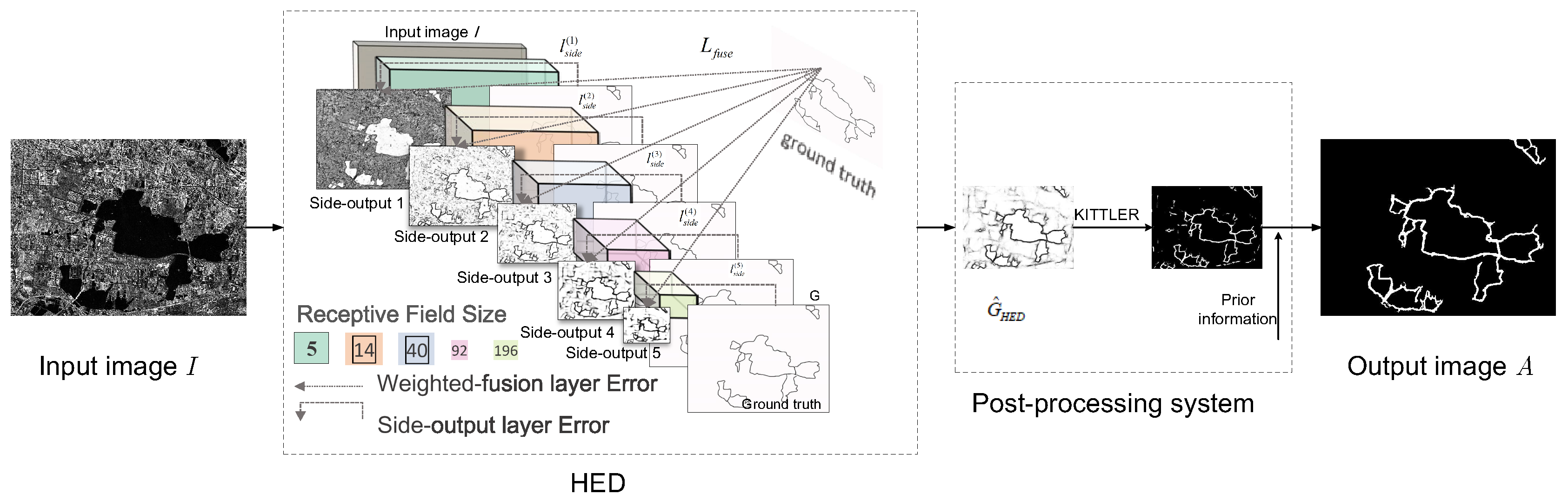
A post-processing system is added to modify the HED algorithm. The modified HED can output the binary edge map A of the input image I. The structure of modified HED is shown in Figure 1; it consists of the original HED and a post-processing system. Before discussing the post-processing system, we first introduce HED.

HED is an end-to-end edge prediction algorithm based on the fully convolutional neural network and deeply supervised nets. This algorithm completes the prediction from image to image through a deep learning model and completes the edge detection for details by multilevel and multi-scale feature learning. HED incorporates two improvements upon VGG-Net. First, as it is advantageous to obtain multiple prediction results and then fuse all the edge maps, HED connects the side-output layer to the last convolutional layer in each stage, respectively conv1_2, conv2_2, conv3_3, conv4_3 and conv5_3. The side-output layer is implemented as a convolution layer with 1 kernel and 1 output. Therefore, the size of the receptive field of each convolutional layer is the same as the corresponding side-output layer. Second, to obtain meaningful side-output results and reduce the memorytime cost, HED cuts the fifth pooling layer and all the fully connected layers of the VGG-Net. The completed HED network architecture includes 5 stages with strides of 1, 2, 4, 8, and 16, respectively, and all nested in the VGG-Net with different receptive field sizes. The network architecture of HED is shown in Figure 1, the network is trained with multiple error propagation paths. The five side-output layer of HED are inserted after the convolutional layer respectively, and deep supervision is imposed at each side-output layer, so that the result is toward the edge detection. At the same time, as the size of side-output layer becomes smaller, the receptive field becomes larger. Finally, the output of HED is obtained through a weighted fusion layer from multi-scale outputs.

The detailed formulation for HED training and testing is given here. During the training process, the goal is to obtain a network which can learn features to produce edge maps approaching the ground truth. HED defines an image-level loss function $l_{side}$ for the side-outputs and uses $w=(w^{\left(1\right)},\dots ,w^{\left(M\right)})$ to represent the weights of the classifiers. In this equation, each weight corresponds to a side-output layer, M represents the number of side-output layers, and W represents the collection of the other network parameters. The objective function is

$$L_{side}(W,w)=\sum _{m=1}^M{\alpha }_m{l}_{side}^{\left(m\right)}(W,w^{\left(m\right)})$$

(1)

Only 10% of the ground truth consists of edge pixels, which causes a bias problem between the edge and non-edge pixels. To solve this problem, HED introduces a class-balancing weight $\beta$ to define the following class-balanced cross-entropy loss function:

$${\ell }_{side}^{\left(m\right)}(W,w^{\left(m\right)})=-\beta \sum _{j\in G_{+}}logPr(g_j=1|I;W,w^{\left(m\right)})-(1-\beta )\sum _{j\in G_{-}}logPr(g_j=0|I;W,w^{\left(m\right)})$$

(2)

where I represents the original image, G represents the corresponding ground truth, $|G_{-}|$ and $|G_{+}|$ represent the edge and non-edge pixels, respectively, and $\beta =\frac{|G_{-}|}{|G_{-}|+|G_{+}|}$. $Pr(g_j=1|I;W,w^{\left(m\right)})=\sigma (a_j^m)\in [0,1]$ is calculated by the sigmoid function $\sigma (·)$ on the activation value at pixel j.

To use the prediction results of each side-output layer, HED adds a “weight-fusion” layer to connect all the prediction results and learn the fusion weight during the training process. $h=(h_1,\dots ,h_M)$ is denoted as the fusion weight, and the loss function of the fusion layer is

$$L_{fuse}(W,w,h)=Dist(G,{\widehat{G}}_{fuse})$$

(3)

In this equation, ${\widehat{G}}_{fuse}=\sigma ({\sum }_{m=1}^M{h}_m{\widehat{A}}_{side}^{\left(m\right)})$ where ${\widehat{A}}_{side}^{\left(m\right)}=\{a_j^{\left(m\right)},j=1,\dots ,\left|G\right|\}$ are activations of the side-output of layer m. Then, the total loss function is:

$$L(W,w,h)=L_{side}(W,w)+L_{fuse}(W,w,h)$$

(4)

Through HED, we obtain the greyscale edge map ${\widehat{G}}_{HED}$ and insert it into the post-processing system. In the post-treatment system, it is important to extract the edge pixels and filter out the non-edge pixels, which directly affect the results of the image registration.

There are two stages in the post-processing system; in the first stage, we use the KITTLER [48] algorithm to calculate the threshold. We assume that the edge pixel is the target, that the non-edge pixel is the background, and that these pixels satisfy a mixed Gaussian distribution. We calculate the mean and variance of the target and background. Then, based on the minimum classification error, the minimum error objective function (7) is obtained. In these formulations, $h\left(g\right)$ is the grey-level histogram of ${\widehat{G}}_{HED}$.

$${\mu }_i\left(T\right)=\left[\sum _{g=a}^{b}h\left(g\right)\right]/P_i\left(T\right)$$

(5)

$${\sigma }_i^2\left(T\right)=\left[\sum _{g=a}^b{\{g-{\mu }_i\left(T\right)\}}^{2}h\left(g\right)\right]/P_i\left(T\right)$$

(6)

where $a=\left\{\begin{array}{cc}0& i=1\\ T+1& i=2\end{array}\right.$ and $b=\left\{\begin{array}{cc}T& i=1\\ n& i=2\end{array}\right.$.

$$J\left(T\right)=1+2[P_1\left(T\right)log{\sigma }_1\left(T\right)+P_2\left(T\right)log{\sigma }_2\left(T\right)]-2[P_1\left(T\right)log{P}_1\left(T\right)+P_2\left(T\right)log{P}_2\left(T\right)]$$

(7)

The optimal threshold $\tau$ satisfies the following:

$$J\left(\tau \right)=\underset{\tau }{min}J\left(T\right)$$

(8)

We divide the image into binary images by the threshold $\tau$. Then, in the second stage, we introduce the prior information such as the length and position of the edge to filter out the wrong edges. Finally, the post-processing system outputs the binarized edge image A of the original image I.

2.2. FDCM

Chamfer matching is a popular shape-based object detection method; it is usually used in the image matching of two edge maps. Although this method can tolerate small distortions and rotations, it ignores the orientations of the edge pixels. To improve the robustness of chamfer matching, several modified chamfer matching techniques have been proposed, such as orientation chamfer matching (OCM) and directional chamfer matching (DCM).

DCM matches directional edge pixels by using a three-dimensional distance transform. We denote $U=\{u_i\}$ as the template sets and $B=\{b_i\}$ as the query image edge map sets. For each edge pixel x, we denote $\varphi \left(x\right)$ as its orientation, and $\varphi \left(x\right)$ is computed at modulo $\pi$. The DCM score is

$$d_{DCM}(U,B)=\frac{1}{n}\sum _{u_i\in U}\underset{b_j\in B}{min}|u_i-b_j|+\lambda |\varphi (u_i)-\varphi (b_j)|$$

(9)

where $\lambda$ represents a weighting factor between the location and orientation terms.

To reduce the computational burden, FDCM has incorporated several optimal methods. First, it uses a variant RANSAC algorithm to extract line segments from the edge map, and it denotes all of the line segments in the template as $L_U={\{l_{[s_j,e_j]}\}}_{j=1,\dots ,m}$, where $s_j$ and $e_j$ represent the start and end locations of the j-th line, respectively. Thus, the noise is filtered, and the remaining points have a certain structure and support. Second, FDCM proposes a three-dimensional distance transformation to increase the matching speed. Specifically, FDCM quantizes the orientation into q discrete channels $\widehat{\mathsf{\Phi }}=\{{\widehat{\varphi }}_i\}$ evenly in the range [0 π) and sets the quantized edge orientations as the third dimension of a three-dimensional image tensor, where the locations are the first two dimensions of the tensor. Then, the distance from each entry in this tensor to an edge point in the joint location and orientation space is

$$DT{3}_B(x,\varphi \left(x\right))=\underset{b_i\in B}{min}|x-b_j|+\lambda |\widehat{\varphi }\left(x\right)-\widehat{\varphi }\left(b_j\right)|$$

(10)

where $\widehat{\varphi }\left(x\right)$ is the nearest quantization level in the orientation space to $\varphi \left(x\right)$ in $\widehat{\mathsf{\Phi }}$. Then, the DCM matching score of template U and query image B becomes

$$d_{DCM}(U,B)=\frac{1}{n}\sum _{u_i\in U}DT{3}_B(u_i,\widehat{\varphi }(u_i))$$

(11)

Third, FDCM assumes that the directions of all the line segments $L_U$ are the same as the q discrete channels $\widehat{\mathsf{\Phi }}$. FDCM rearranges the DCM matching score as follows:

$$d_{DCM}(U,B)=\frac{1}{n}\sum _{l_j\in L_U}\sum _{u_i\in l_j}DT{3}_B(u_i,\widehat{\varphi }\left(l_j\right))$$

(12)

FDCM computes the distance transformation along each direction and saves the integral distance transform as a tensor, which is denoted as $IDT{3}_B$. Then, each element of $IDT{3}_B$ is

$$IDT{3}_B(x,{\widehat{\varphi }}_i)=\sum _{x_j\in l_{[x_0,x]}}DT{3}_B(x_j,{\widehat{\varphi }}_i)$$

(13)

where $l_{[x_0,x]}$ represents the line with direction $\widehat{{\varphi }_i}$, and $x_0$ is the intersection of the image boundary and this line. Thus, the DCM matching distance score becomes

$$d_{DCM}(U,B)=\frac{1}{n}\sum _{l_{[s_j,e_j]}\in L_U}[IDT{3}_B(e_j,\widehat{\varphi }(l_{[s_j,e_j]}))-IDT{3}_B(s_j,\widehat{\varphi }(l_{[s_j,e_j]}))]$$

(14)

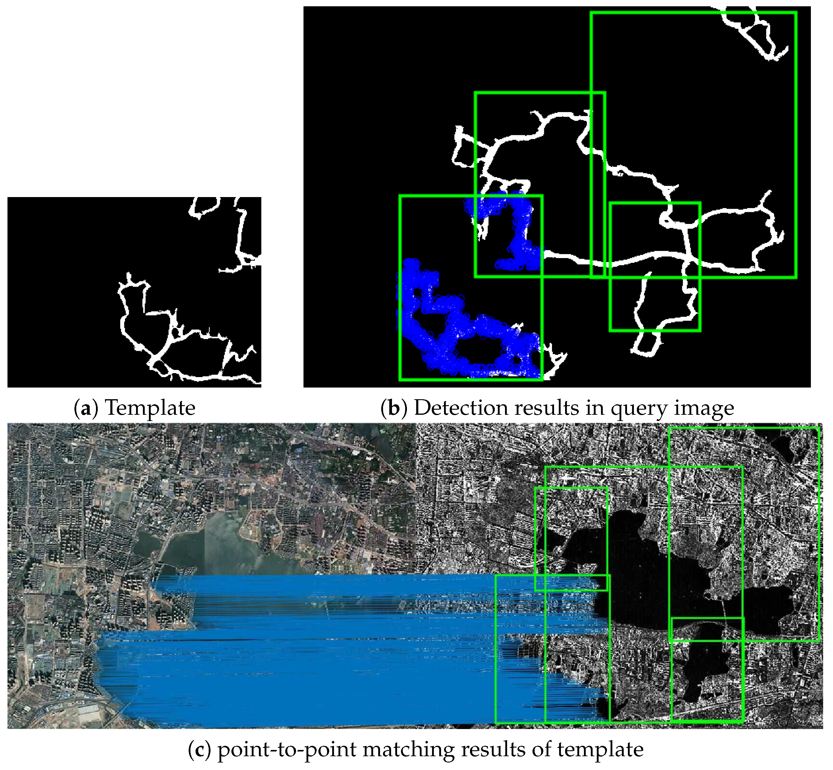
Finally, FDCM sets the matching cost threshold and obtains the results of the shape detection, as shown in Figure 2. Figure 2a shows the template, and the green box in Figure 2b represents the matched shape location. The locations of each point $u_i\in U$ and its nearest edge point in V are output; and then, these points are matched one by one. In Figure 2b, the blue points show the nearest edge points of $u_i\in U$. Figure 2c shows the point-to-point matching results of this template and query image on the optical and SAR images.

2.3. Mesh Grid Strategy

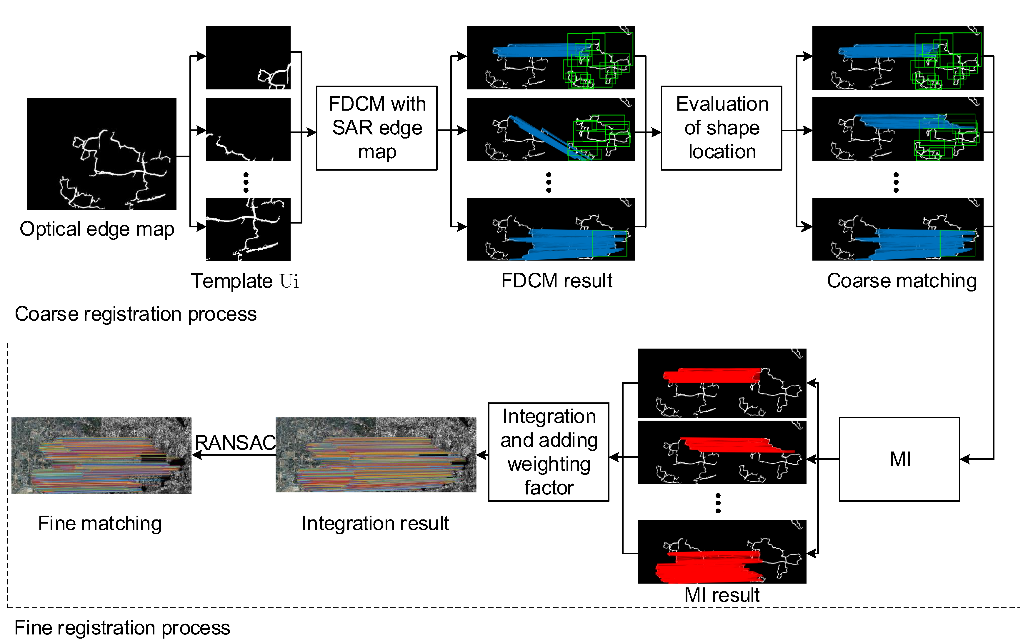
A mesh grid strategy is employed to perform a coarse-to-fine image registration, as shown in Figure 3. The upper part of Figure 3 shows the coarse registration process. In this process, the optical edge map is first divided into N templates; then, FDCM is introduced to obtain the matching points between the SAR edge map and the template. After estimating the matching points of all the grids, the wrongly detected shape locations can be corrected and the coarse matching result is obtained. The lower part of Figure 3 shows the fine registration process. In this process, MI is introduced to fine-tune the coarse matching result; then, matching points are integrated, and a weighting factor is added to each grid. Finally, RANSAC is introduced to obtain a fine matching result.

The mesh grid strategy is given in detail here. First, the optical edge map A is divided into N mesh grids, where $U_i(i=1,2,\dots ,N)$ represents the i-th grid, which can be used as a template for the FDCM. Let the SAR edge map be denoted as B. Then, FDCM is used to calculate the matching points between $U_i$ and B.

However, FDCM is usually used for shape-based object detection. When it is used to match points, there are two problems: first, it can detect all the shapes that resemble the template, which makes it difficult to determine whether the corresponding matching location has the minimum cost. Second, the point in the template and its corresponding nearest point in the query image are not always correctly matched. As a result, the corresponding shape cannot always be detected.

The mesh grid strategy can be used to solve these two problems. We denote the matching points location of template $U_i$ as $L{(A,U_i)}_{[s_j,e_j]}$, and its corresponding nearest points location is denoted as $L{(B_i)}_{[s_j,e_j]}$. In the coarse registration process, after we obtain the matching points between $U_i$ and B, we calculate their coordinates transformation in N grids. There is similarity between the point coordinates transformation of different grids within a certain threshold. Then, the wrong matching is determined, and the correct location is obtained according to the matching results of the other grids.

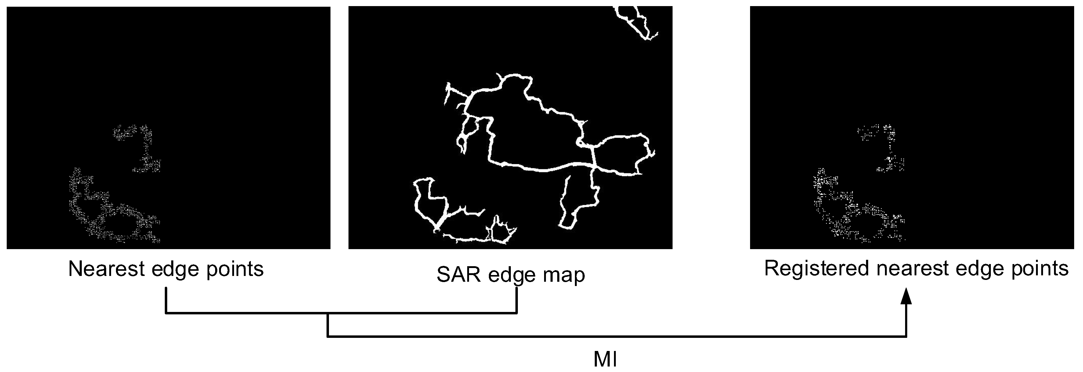
Second, as the nearest edge points’ locations $L{(B_i)}_{[s_j,e_j]}$ are known, MI is introduced to register the nearest edge points and their corresponding region in the SAR edge map, as shown in Figure 4. Thus, we can calculate the nearest coordinates after the transformation, and we denote them as $L^{\prime }{(B_i)}_{[s_j,e_j]}$. Third, we add a weighting factor $\delta$ to each grid. For each template $U_i$, if there is no correct matching location for all of the detection boxes in B obtained by FDCM, we set ${\delta }_i=0$; otherwise, ${\delta }_i=1$, and the matching points in optical edge image A are

$$L_{A_{[s_j,e_j]}}=\sum _{i=1}^N{\delta }_i\ast L{(A,U_i)}_{[s_j,e_j]}.$$

(15)

The matching points in optical edge image B are

$$L_{B_{[s_j,e_j]}}=\sum _{i=1}^N{\delta }_i\ast L^{\prime }{(B_i)}_{[s_j,e_j]}.$$

(16)

Finally, RANSAC is introduced to fine-tune the integrated points matching to obtain a fine matching result. In this stage, note that there is parallax between images; we can set a loose threshold for RANSAC, then introduce moving DLT.

2.4. Moving DLT

When there is parallax or distortion in the images, using a homography matrix for the homography warp will result in misalignment. We solve this problem by drawing on the experience of APAP [46]: the image is divided into several cells, then the homography matrix of each cell is calculated to align all the pixels in this cell. The matrix is calculated by moving DLT.

If we assumed that there is a feature point $x\in L_B$ in the SAR image, its corresponding matching points in the optical image will be $x^{\prime }\in L_A$. Furthermore, the homogeneous coordinates of the two points are marked as $\tilde{x}={\left[\begin{array}{ccc}s& e& 1\end{array}\right]}^T$ and ${\tilde{x}}^{\prime }={\left[\begin{array}{ccc}{s}^{\prime }& e^{\prime }& 1\end{array}\right]}^T$, and the following mapping relationship between them is satisfied:

$${\tilde{x}}^{\prime }\sim H\tilde{x}$$

(17)

In non-homogeneous coordinates, the j-th row of matrix H is recorded as $r_j$. Then, the coordinates of the map satisfy the following formula:

$${\tilde{s}}^{\prime }=\frac{r_1{\left[\begin{array}{ccc}s& e& 1\end{array}\right]}^T}{r_3{\left[\begin{array}{ccc}s& e& 1\end{array}\right]}^T} and {\tilde{e}}^{\prime }=\frac{r_2{\left[\begin{array}{ccc}s& e& 1\end{array}\right]}^T}{r_3{\left[\begin{array}{ccc}s& e& 1\end{array}\right]}^T}$$

(18)

DLT is a basic algorithm for computing homography matrix H: by substituting $\tilde{x}$ and ${\tilde{s}}^{\prime }$ into the formula $0_{3\times 1}={\tilde{x}}^{\prime }\times H\tilde{x}$, we obtain

$$0_{3\times 1}=\left[\begin{array}{ccc}{0}_{1\times 3}& -{\tilde{x}}^T& y^{\prime }\tilde{x}{}^T\\ {\tilde{x}}^T& 0_{1\times 3}& -x^{\prime }{\tilde{x}}^T\\ -y^{\prime }{\tilde{x}}^T& x^{\prime }{\tilde{x}}^T& 0_{1\times 3}\end{array}\right]h,h=\left[\begin{array}{c}{r_1}^T\\ {r_2}^T\\ {r_3}^T\end{array}\right]$$

(19)

where h is the vector obtained by the vectorization of H. Set the first two lines of the upper matrix as $a_j\in R^{2\times 9}$ and let j represent the j-th matching point pair. Then, the objective function of matrix H is

$$\widehat{h}=\underset{h}{argmin}\sum _{j=1}^N{∥a_{j}h∥}^{2}s.t.∥h∥=1$$

(20)

After rearranging $h$, we obtain the homography matrix H. Once this matrix has been obtained, the other pixels in the image can be linearly transformed according to it. The moving DLT algorithm uses a weighted value to estimate the homography matrix based on DLT. We set the coordinates of the center points of each cell as $x_{\ast }$, and the corresponding cells of the two images satisfy the following condition:

$${{\tilde{x}}_{\ast }}^{\prime }\sim H_{\ast }{{\tilde{x}}_{\ast }}^{\prime }$$

(21)

$H_{\ast }$ is estimated by the following formula:

$$h_{\ast }=\underset{h}{argmin}\sum _{j=1}^n{∥{\omega }_{\ast }^j{a}_{j}h∥}^{2}s.t.∥h∥=1$$

(22)

where ${\{{\omega }_{\ast }^j\}}_{j=1}^N\in [0,1]$ is positively related to the geometric distance between each pixel $x_{\ast }$ and the j-th matching point $x_j$ in the picture. To avoid the error of having $\omega$ be too close to 0, we set a small value $\gamma \in [0,1]$ to offset the weights:

$${\omega }_{\ast }^i=max(exp(-||x_{\ast }-x_j|{|}^2/{\sigma }^2),\gamma )$$

(23)

3. Framework of the Point Pattern Chamfer Registration Based on Mesh Grids

A point pattern chamfer registration method based on mesh grids (PPCM) is proposed in this paper; its overall framework is shown in Figure 5. First, to eliminate the effects of noise in the SAR image and the differences in the greyscale and resolution between the optical and SAR image, the main edge contour of the image is extracted by our modified HED algorithm. Second, due to the edge distribution and computation cost, we set $N=4$ to divide the edge of the optical image into 4 grids. For each grid, a template is obtained, FDCM is introduced to complete the matching of the template and the SAR image, and the matching result of each mesh grid is evaluated to obtain a coarse matching result. Third, MI is employed to fine-tune the results. Hence, we obtain the fine matching result of the two images after adding a weighting factor and applying the RANSAC algorithm. Finally, we complete the registration of the optical and SAR images by using moving DLT to align the SAR images.

4. Experiment

In this section, we first show the three sets of optical and SAR images which are designed to evaluate the proposed method. Then, the output of the intermediate steps of the algorithm and the final registered images are displayed. Finally, the matching correctness of feature points and the root mean square error (RMSE) [49] of registered images are calculated to evaluate the accuracy and robustness of our proposed algorithm.

4.1. Experiment Data

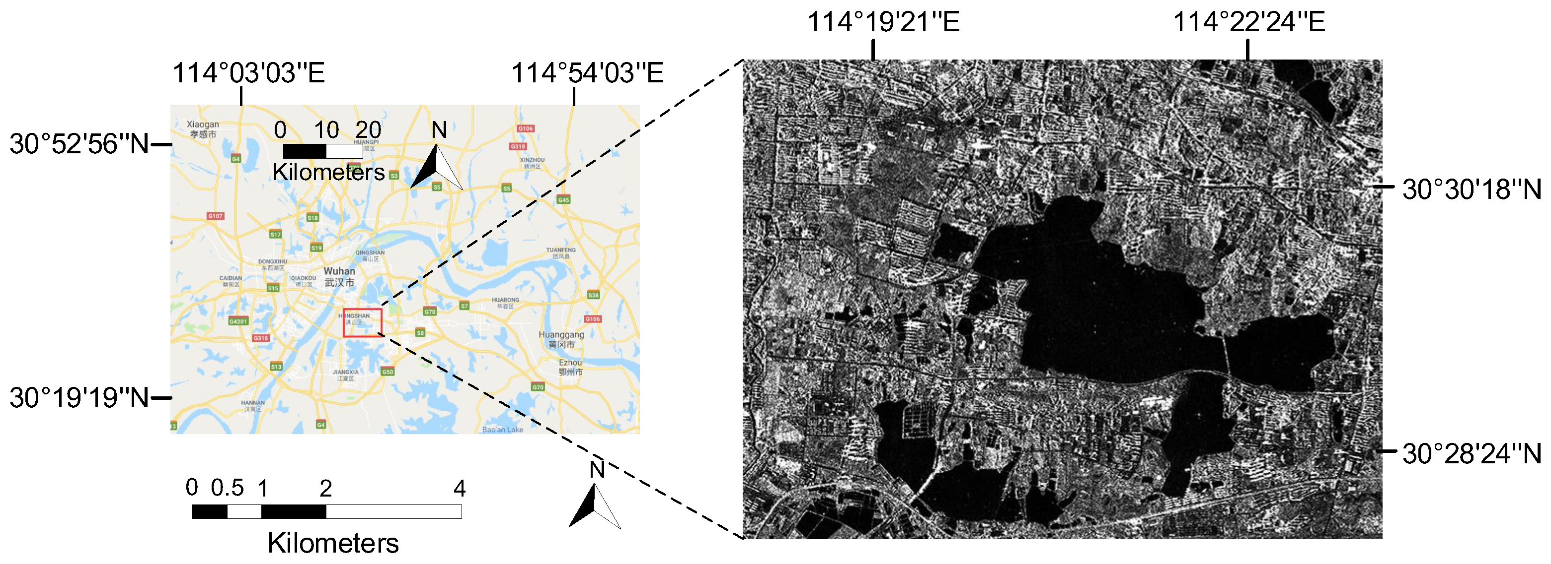
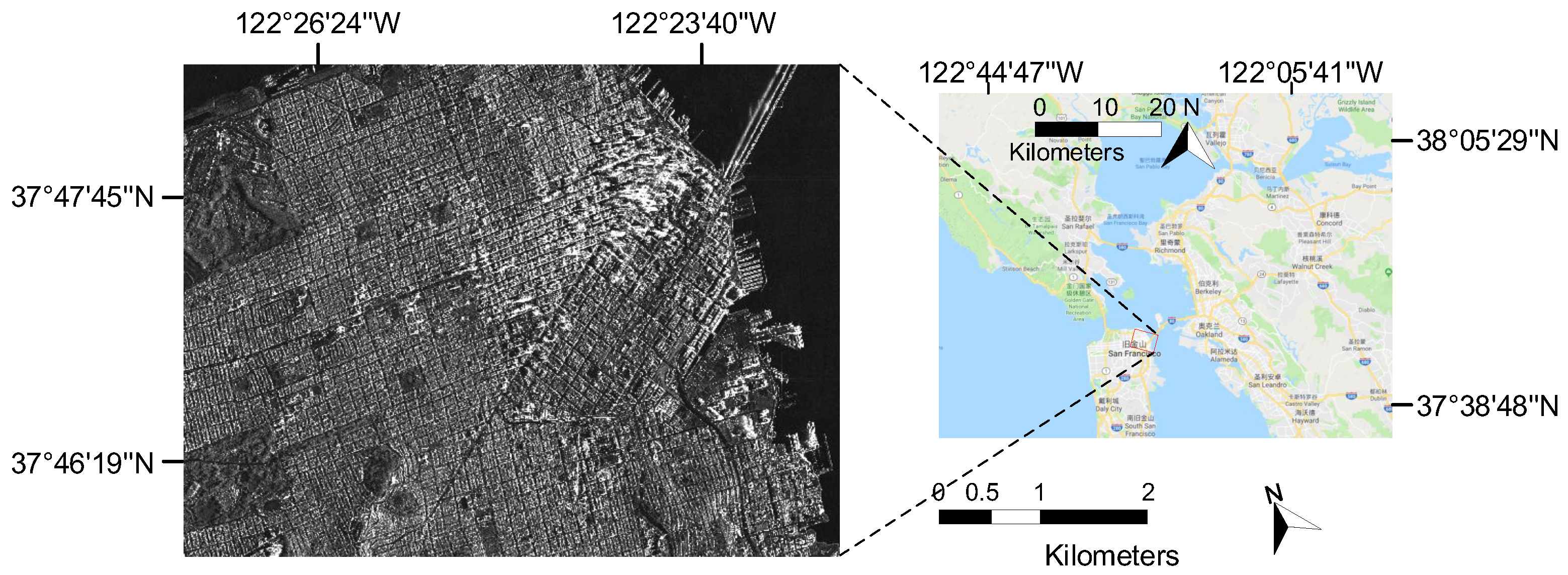
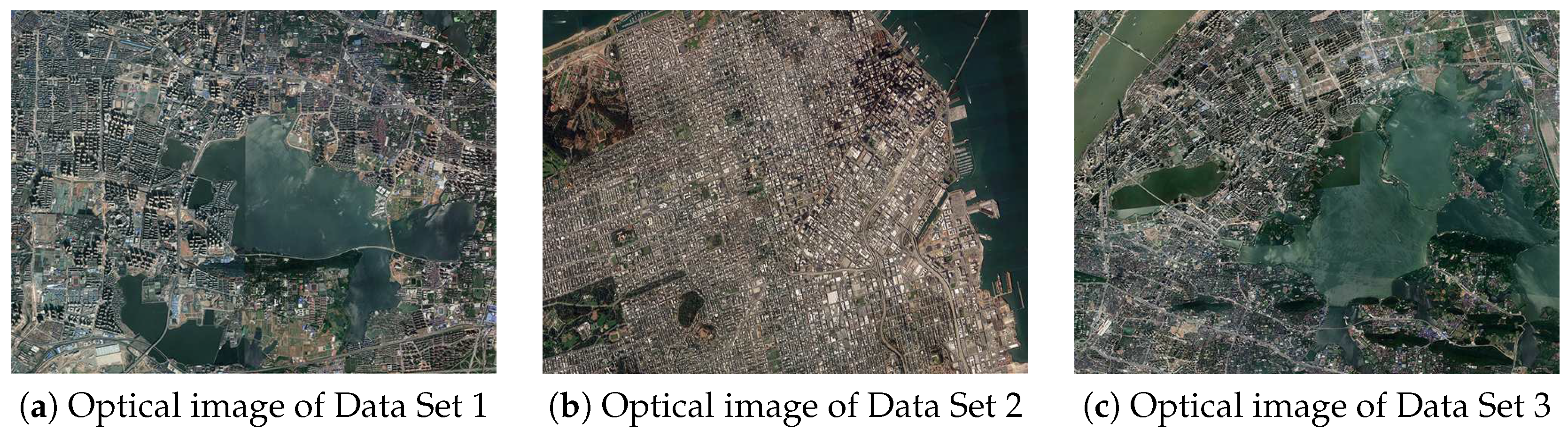
In the registration experiments, three sets of data are used to evaluate our proposed method, and details of these tested images are listed in

Table 1. Experimental images and their characteristics.

Data Set	Sensor	Resolutions	Position	Date	Size
Data Set 1	TerraSAR-X (VV polarization)	1.75 m	Wuhan	28 September 2008	3040 × 2481
	Google Earth	17 m	Wuhan	5 May 2017	998 × 819
Data Set 2	TerraSAR-X (HH polarization)	0.455 m × 0.872 m	San Francisco	2 October 2011	782 × 510
	Google Earth	8 m	San Francisco	11 May 2018	2126 × 1388
Data Set 3	TerraSAR-X (VV polarization)	1.75 m	Wuhan	28 September 2008	1020 × 772
	Google Earth	8 m	Wuhan	9 December 2017	3048 × 2252

. For Data Set 1, the study area is within Wuhan City, Hubei Province, China. The SAR image are single polarized (VV channel) data acquired by the TerraSAR-X, its near incidence angle is 34.074 degree, and the far incidence angle is 35.486 degree, as shown in Figure 6. The scaling difference between tested images is close to 10 times and the time interval is nearly 9 years. The SAR image of Data Set 2 is presented in Figure 7, it is single polarized (HH channel) Terra-SAR data acquired in San Francisco, the United States, the near incidence angle is 39.557 degree and the far incidence angle is 40.162 degree. The tested images are captured with a difference of 7 years. For last set of experiment data, the SAR image has the same resolution, incidence angle and acquisition time with the SAR image of the first data set, the specific location is shown in Figure 8. The resolution between tested images is nearly 5 times and the time interval reaches 9 years. The optical images of these three experiment data sets are downloaded from Google Earth, they are displayed in Figure 9.

4.2. Experiment Result

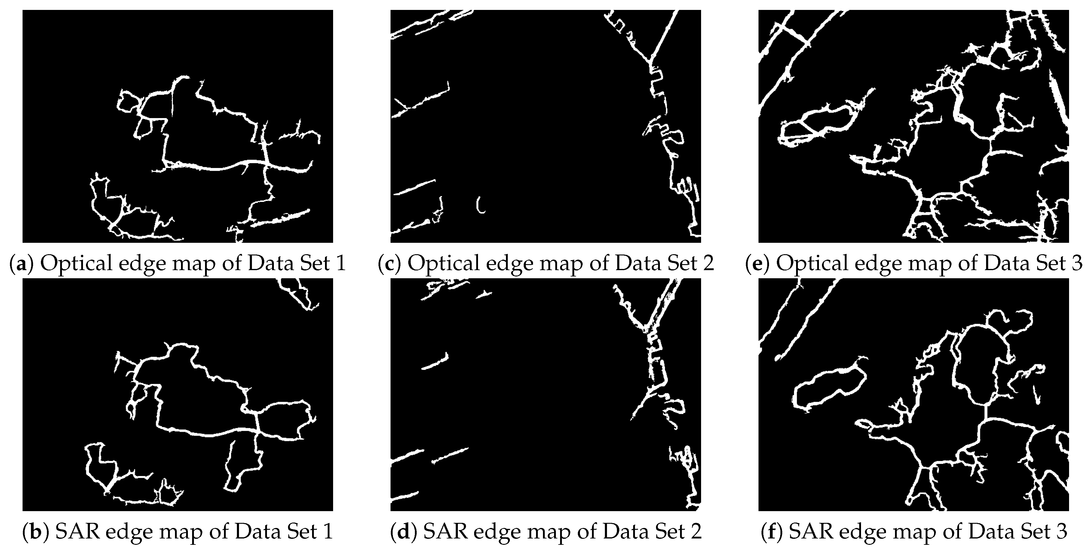
First, all images are resized to 640 × 480, and the modified HED is used to obtain their edge maps of the original optical image and the SAR image. The output edge map is presented in Figure 10.

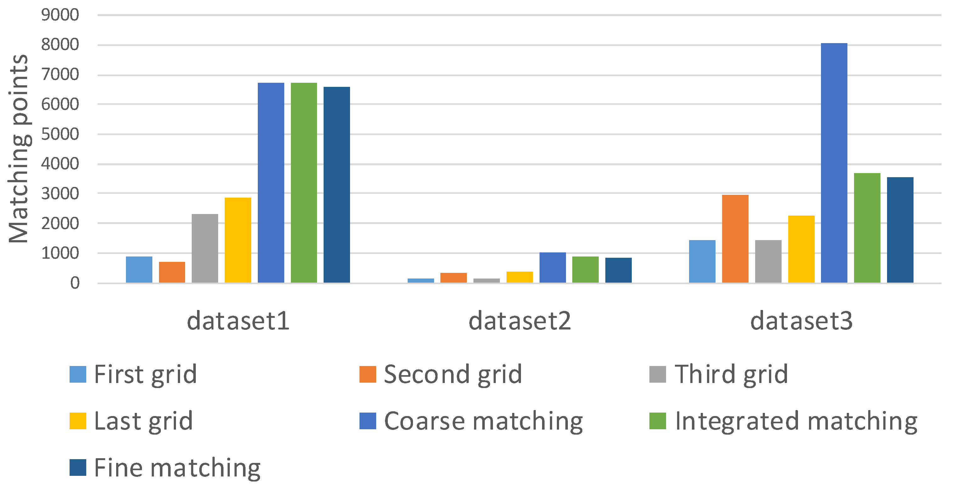
The matching points obtained from the distinct grids are calculated as shown in

Table 2. Point matching results by different methods.

Matching Points	First Grid	Second Grid	Third Grid	Last Grid	Coarse Matching	Integrated Matching	Fine Matching
Data Set 1	896	680	2284	2852	6712	6712	6574
Data Set 2	156	346	148	370	1020	864	851
Data Set 3	1442	2934	1454	2254	8084	3708	3545

; the number of the matching points in each grid, the matching points obtained by coarse matching and fine matching, and the number of integrated matching points before RANSAC are listed. For Data Set 1, the matching results of each grid are evaluated, and the correct matching result of the 2-nd grid is determined; then, MI is used to fine-tune the coarse matching result and the weighting factor is calculated, ${\delta }_1={\delta }_2={\delta }_3={\delta }_4=1$. For Data Set 2, we set ${\delta }_1=0$, ${\delta }_2={\delta }_3={\delta }_4=1$. For Data Set 3, we set ${\delta }_1={\delta }_2=0$, ${\delta }_3={\delta }_4=1$. Figure 11 depicts the statistical results of the three sets of data.

The number of matching points of each grid is related to the number of contour pixels in that grid, and the matching ratio between the template and the SAR image. Because the number of matching points of each grid in an image is close, the weight of each grid is nearly equal. Thus, this approach will help us to determine the correct matching location in the process of estimation and integration.

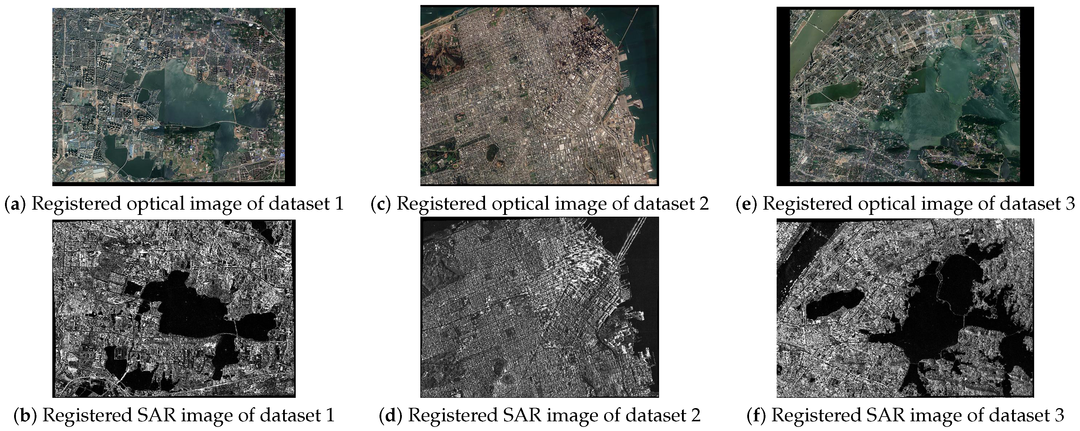
The final results of the image registration is shown in Figure 12. To permit convenient comparison and observation, the optical images and the registered SAR images are displayed in the same coordinate system.

4.2.1. Correct Matching Ratio Comparison

To evaluate the correct matching ratio of our proposed method, PSO-SIFT [42] and the joint spectral correspondence for disparate image matching (JSCM) [50] are chosen for comparison. PSO-SIFT can be applied to register multi-spectral and multi-sensor remote sensing images, including Landsat, optical and SAR images. It defined a new gradient and enhanced the feature matching method to increase the accuracy of matching. JSCM can be applied to match images with disparate appearance, such as dramatic illumination, age and rendering style differences. It analyzes the eigen-spectrum of the joint image graph constructed from all the pixels in the two images to match persistent features between them. Considering that the time interval of our experiment data sets may cause differences of features, JSCM is chosen as a comparison method for evaluating points matching correctness, although it is not used for registration of the optical images and the SAR images. The results are shown in

Table 3. Point matching results by different methods.

Dataset	Matching Results	PSO-SIFT	JSCM	Proposed Method (PPCM)
Data Set 1	Initial matches	40	11	6712
	Correct matches	0	5	6574
	matching ratio	0	0.4545	0.9794
Data Set 2	Initial matches	18	9	864
	Correct matches	0	5	851
	matching ratio	0	0.5556	0.9850
Data Set 3	Initial matches	39	16	3708
	Correct matches	0	10	3545
	matching ratio	0	0.6250	0.9560

.

According to the results in Table 3, PSO-SIFT fails to detect and match feature points between the optical and SAR images; JSCM obtains several correct matches, while PPCM obtains a large number of matching points and has the highest matching correctness among these three methods.

4.2.2. Registration Performance Comparison

To evaluate the registration results of PPCM, four methods are chosen for comparison. Based on MI [6], the first method maximizes the MI between the optical and SAR image to complete optical-to-SAR image registration. The second method is PSO-SIFT (position scale orientation SIFT) [42], widely used in multi-spectral and multi-sensor remote sensing images registration with modified SIFT and enhanced feature matching. A RACM [14], which is based on edge features and MI to complete the optical-to-SAR image registration, is chosen to be the third comparison method. The last method for comparison is a global warping plus the points matching results obtained by our proposed method. The registration results are estimated by calculating the RMSE [49] of the two images after registration. The RMSE is computed by the following formula:

$$\mathrm{RMSE}=\sqrt{\frac{1}{n}\sum _{i=1}^n[{({x_B}_i-x_{Ai})}^2+{(y_{Bi}-y_{Ai})}^2]}$$

(24)

Since the estimation results are affected by the number and location of the control points, 5 and 30 pairs of control points are respectively selected for estimation. The results are summarized in

Table 4. Quantitative comparisons.

Data Set			MI	PSO-SIFT	RACM	Matching Result + Global Warping	Proposed Method
Data Set 1	RMSE	5	8.3427	/	16.2911	4.7958	4.7117
		30	10.0283	/	20.8854	7.1157	5.1704
	time (s)		101.4491	/	86.6159	72.8378	113.6955
Data Set 2	RMSE	5	77.0766	/	8.1564	8.2183	8.4971
		30	80.9856	/	10.3005	9.4498	9.1378
	time (s)		34.0148	/	75.335	28.6711	39.5018
Data Set 3	RMSE	5	23.3152	/	27.4299	17.3090	13.5527
		30	22.4061	/	21.7394	16.4874	12.0153
	time (s)		170.7673	/	376.4573	57.7867	82.5684

.

To analyze the matching results, comparing the optical images and the SAR images in the three sets of data may be helpful. For Data Set 1, there is a gradient change in the middle of the image caused by illumination or other imaging conditions, thus, the feature detector tends to extract the extra lines. Brightness changes also exists in the optical image of Data Set 3. For Data Set 2, the straight-line features are obvious, and the geometric distortion is very small, while the straight-line edges of the first set of data and the third set of data are not obvious. For Data Set 3, there are geometric distortions between the optical and SAR images. In fact, intrinsic and distinct differences exist in the optical and SAR images, with time interval and resolution differences in testing images added, registration becomes more difficult.

From Table 4, it can be seen that the PSO-SIFT algorithm cannot complete the registration of the three groups of images. After combining the results of matching pairs in Table 3, it is clear that PSO-SIFT detects 0 correct matching points. In PSO-SIFT algorithm, after defining a new gradient to overcome the difference of image intensity between the two images, the histograms of scale ratio, horizontal shifts, and vertical shifts of the matched key points are expected to only have a single mode. However, it can be inferred that this new gradient is ineffective for our three experiment data sets by observing the histograms. By applying PSO-SIFT on resized testing images and images with short time interval, it can be speculated two reasons for the failure of the PSO-SIFT algorithm. First, even though improved, SIFT is not robust enough to detect and match feature points between the optical and SAR image due to their intrinsic differences [41]. Second, SIFT-based methods are not suitable to register large size and high-resolution SAR images since they are proposed for small-size images [51]. In addition, the differences of resolution and time interval will increase the difficulty of registration. Furthermore, the geometric deformation can also affect the registration results.

MI can complete the registration of the first and third data sets, but it cannot register Data Set2. There may be two reasons for the failure of MI-based method. One is that the registration results obtained by MI can be trapped into a local optimum; the other is that the registration of MI is based on the intensity of the image. Thus, MI will be ineffective when the change in the information entropy is not obvious. For RACM, it performs well on Data Set 2, but has a low accuracy on the first and third data sets. RACM is based on edge features and MI, and its application has two limitations. First, the edge detection results determines the accuracy of the registration, but the edge detection methods used in RACM is sensitive to speckle noises and edges, which will have a negative influence on the accuracy of registration. Second, RACM is insufficient in solving the geometric distortions.

The comparison result of our proposed method and a global image warping based on the point matching results obtained by our proposed method are listed in Table 4, the moving DLT has better accuracy than the global image alignment, especially in the third set of data with geometric distortion. Both methods obtain more accurate results than the other three methods and prove that PPCM has good robustness.

The running times of five methods are also listed in Table 4. The computation complexity of PPCM depends on the distribution of edges and the number of points on the edge, moving DLT has a larger amount of computation cost than a global warping. Moreover, the computation cost of MI and RACM become large while registering the remote sensing image with large size. As the image size increases, PPCM has less computation cost than other comparison methods, because PPCM resizes the image before the main contour is extracted by the modified HED. Since PPCM extracts the main contour as matching primitive and ignores other areas, the image size change has no effect on feature matching. The calculation time of our proposed method in Table 4 has added the time of image resizing.

4.3. Discussion

For these three image pairs, PPCM completes the registration of all the datasets and has the minimum error, it is more robust than other comparison methods. There are three main contributions in our proposed method: (1) Traditional edge-based optical-to-SAR registration methods usually extract almost all the edges. In contrast, PPCM introduces modified HED to extract the main contour of image pairs so that it is not influenced by local features and speckle noises, especially for image pairs which have differences of resolutions and acquisition time. (2) The mesh grid strategy proposed by PPCM can perform a coarse-to-fine registration and solve small geometric distortions. This strategy selects the point matching result of FDCM and integrates all the matching pairs to complete a point pattern chamfer matching. Then, PPCM can obtain a large amount of feature points, while the traditional feature-based algorithms detect a small number of correct feature matches. (3) Based on the large amount of matching points obtained by PPCM, moving DLT is introduced to complete the image alignment.

However, there are still some limitations in our proposed method. The major limitation is that PPCM would be not that robust when applied to mountainous area without main contours. Second, for small-size images, the computation cost of the proposed method is larger than other similar optical-to-SAR image registration methods. Furthermore, PPCM still has difficulty in registering images with large geometric distortions. Therefore, our future work includes three aspects: (1) Extracting better contours to complete more robust registration for areas without obvious contours. (2) Finding a flexible way to mesh grids, for example, grids associated with contours can be helpful for solving large geometric distortions. (3) Obtaining more concise contour information to reduce the computation cost.

5. Conclusions

In this paper, a new optical-to-SAR image registration framework called PPCM is proposed. In PPCM algorithm, a modified HED algorithm is used to extract the main contour edge map from the images, and FDCM is used to calculate the matching points of each template and SAR image. First, the mesh grid strategy provides the templates required for FDCM and evaluates the fast directional chamfer matching results to obtain a coarse matching result. Then, the strategy introduces MI and integrates the matching results. Finally, our strategy introduces RANSAC to obtain the fine matching result. The experimental results show that our proposed method can complete the optical-to-SAR image registration with small geometric distortions and thereby proves its effectiveness and accuracy. However, there is still a major limitation of the algorithm, when applied to forests or mountains in which obvious contour does not exist, the proposed method will be no longer robust, since it extracts the main contour as the matching primitive. Enhancing the robustness of our proposed method for areas without obvious contour and reducing its computation cost are the goals of our future work.

References

- Brown, L.G. A survey of image registration techniques. ACM Comput. Surv. 1992, 24, 325–376. [Google Scholar] [CrossRef] [Green Version]
- Liesenberg, V.; de Souza Filho, C.R.; Gloaguen, R. Evaluating moisture and geometry effects on L-band SAR classification performance over a tropical rain forest environment. IEEE J. Sel. Top. Appl. Earth Obs. Remote Sens. 2016, 9, 5357–5368. [Google Scholar] [CrossRef]
- Errico, A.; Angelino, C.V.; Cicala, L.; Persechino, G.; Ferrara, C.; Lega, M.; Vallario, A.; Parente, C.; Masi, G.; Gaetano, R. Detection of environmental hazards through the feature-based fusion of optical and SAR data: A case study in southern Italy. Int. J. Remote Sens. 2015, 36, 3345–3367. [Google Scholar] [CrossRef]
- Zhang, G.; Sui, H.; Song, Z.; Hua, F.; Hua, L. Automatic Registration Method of SAR and Optical Image Based on Line Features and Spectral Graph Theory. In Proceedings of the International Conference on Multimedia and Image Processing, Wuhan, China, 17–19 March 2017; pp. 64–67. [Google Scholar]
- Yang, L.J.; Tian, Z.; Zhao, W. A new affine invariant feature extraction method for SAR image registration. Int. J. Remote Sens. 2014, 35, 7219–7229. [Google Scholar] [CrossRef]
- Suri, S.; Reinartz, P. Mutual-Information-Based Registration of TerraSAR-X and Ikonos Imagery in Urban Areas. IEEE Trans. Geosci. Remote Sens. 2010, 48, 939–949. [Google Scholar] [CrossRef]
- Hasan, M.; Pickering, M.R.; Jia, X. Multi-modal registration of SAR and optical satellite images. In Proceedings of the Digital Image Computing: Techniques and Applications, Melbourne, VIC, Australia, 1–3 December 2009; pp. 447–453. [Google Scholar]
- Merkle, N.; Müller, R.; Schwind, P.; Palubinskas, G.; Reinartz, P. A new approach for optical and sar satellite image registration. ISPRS Ann. Photogramm. Remote Sens. Spat. Inf. Sci. 2015, 2, 119. [Google Scholar] [CrossRef]
- Li, W.; Leung, H. A maximum likelihood approach for image registration using control point and intensity. IEEE Trans. Image Process. 2004, 13, 1115–1127. [Google Scholar] [CrossRef] [PubMed]
- Cheah, T.C.; Shanmugam, S.A.; Mann, K.A.L. Medical image registration by maximizing mutual information based on combination of intensity and gradient information. In Proceedings of the 2012 International Conference on Biomedical Engineering (ICoBE), Penang, Malaysia, 27–28 February 2012; pp. 368–372. [Google Scholar]
- Cole-Rhodes, A.A.; Johnson, K.L.; LeMoigne, J.; Zavorin, I. Multiresolution registration of remote sensing imagery by optimization of mutual information using a stochastic gradient. IEEE Trans. Image Process. 2003, 12, 1495–1511. [Google Scholar] [CrossRef] [PubMed] [Green Version]
- Li, Z.; Leung, H. Contour-based multisensor image registration with rigid transformation. In Proceedings of the 2007 10th International Conference on Information Fusion, Quebec, QC, Canada, 9–12 July 2007; pp. 1–7. [Google Scholar]
- Arora, M.K. Mutual information-based image registration for remote sensing data. Int. J. Remote Sens. 2003, 24, 3701–3706. [Google Scholar] [Green Version]
- Saidi, F.; Chen, J.; Wang, P. A refined automatic co-registration method for high-resolution optical and sar images by maximizing mutual information. In Proceedings of the IEEE International Conference on Signal and Image Processing, Beijing, China, 13–15 August 2017; pp. 231–235. [Google Scholar]
- Gong, M.; Zhao, S.; Jiao, L.; Tian, D.; Wang, S. A novel coarse-to-fine scheme for automatic image registration based on SIFT and mutual information. IEEE Trans. Geosci. Remote Sens. 2014, 52, 4328–4338. [Google Scholar] [CrossRef]
- Lowe, D.G. Distinctive Image Features from Scale-Invariant Keypoints. Int. J. Comput. Vis. 2004, 60, 91–110. [Google Scholar] [CrossRef] [Green Version]
- Fan, B.; Huo, C.; Pan, C.; Kong, Q. Registration of optical and SAR satellite images by exploring the spatial relationship of the improved SIFT. IEEE Geosci. Remote Sens. Lett. 2013, 10, 657–661. [Google Scholar] [CrossRef]
- Dellinger, F.; Delon, J.; Gousseau, Y.; Michel, J.; Tupin, F. SAR-SIFT: A SIFT-Like Algorithm for SAR Images. IEEE Trans. Geosci. Remote Sens. 2013, 53, 453–466. [Google Scholar] [CrossRef] [Green Version]
- Schwind, P.; Suri, S.; Reinartz, P.; Siebert, A. Applicability of the SIFT operator to geometric SAR image registration. Int. J. Remote Sens. 2010, 31, 1959–1980. [Google Scholar] [CrossRef]
- Wang, S.; You, H.; Fu, K. BFSIFT: A Novel Method to Find Feature Matches for SAR Image Registration. IEEE Geosci. Remote Sens. Lett. 2012, 9, 649–653. [Google Scholar] [CrossRef]
- Wang, F.; You, H.; Fu, X. Adapted Anisotropic Gaussian SIFT Matching Strategy for SAR Registration. IEEE Geosci. Remote Sens. Lett. 2015, 12, 160–164. [Google Scholar] [CrossRef]
- Fan, J.; Wu, Y.; Wang, F.; Zhang, Q.; Liao, G.; Li, M. SAR Image Registration Using Phase Congruency and Nonlinear Diffusion-Based SIFT. IEEE Geosci. Remote Sens. Lett. 2014, 12, 562–566. [Google Scholar]
- Wang, B.; Zhang, J.; Lu, L.; Huang, G.; Zhao, Z. A Uniform SIFT-Like Algorithm for SAR Image Registration. IEEE Geosci. Remote Sens. Lett. 2015, 12, 1426–1430. [Google Scholar] [CrossRef]
- Xiang, Y.; Wang, F.; Wan, L.; You, H. An Advanced Rotation Invariant Descriptor for SAR Image Registration. Remote Sens. 2017, 9, 686. [Google Scholar] [CrossRef]
- Huang, L.; Li, Z. Feature-based image registration using the shape context. Int. J. Remote Sens. 2010, 31, 2169–2177. [Google Scholar] [CrossRef] [Green Version]
- Li, H.; Manjunath, B.S.; Mitra, S.K. A Contour-Based Approach to Multisensor Image Registration; IEEE Press: Piscataway, NJ, USA, 1995; p. 320. [Google Scholar]
- Pan, C.; Zhang, Z.; Yan, H.; Wu, G.; Ma, S. Multisource data registration based on NURBS description of contours. Int. J. Remote Sens. 2008, 29, 569–591. [Google Scholar] [CrossRef]
- Dare, P.; Dowman, I. An improved model for automatic feature-based registration of SAR and SPOT images. ISPRS J. Photogramm. Remote Sens. 2001, 56, 13–28. [Google Scholar] [CrossRef]
- Canny, J. A Computational Approach to Edge Detection. IEEE Trans. Pattern Anal. Mach. Intell. 1986, PAMI-8, 679–698. [Google Scholar] [CrossRef]
- Gioi, R.G.V.; Jakubowicz, J.; Morel, J.M.; Randall, G. LSD: A line segment detector. Image Process. Line 2012, 2, 35–55. [Google Scholar] [CrossRef]
- Fjortoft, R.; Lopes, A.; Marthon, P.; Cuberocastan, E. An optimal multiedge detector for SAR image segmentation. IEEE Trans. Geosci. Remote Sens. 1998, 36, 793–802. [Google Scholar] [CrossRef] [Green Version]
- Xiang, D.; Ban, Y.; Wang, W.; Tang, T.; Su, Y. Edge Detector for Polarimetric SAR Images Using SIRV Model and Gauss-Shaped Filter. IEEE Geosci. Remote Sens. Lett. 2016, 13, 1661–1665. [Google Scholar] [CrossRef]
- Liu, J.; Scott, K.A.; Gawish, A.; Fieguth, P. Automatic Detection of the Ice Edge in SAR Imagery Using Curvelet Transform and Active Contour. Remote Sens. 2016, 8, 480. [Google Scholar] [CrossRef]
- Xie, S.; Tu, Z. Holistically-Nested Edge Detection. Int. J. Comput. Vis. 2015, 125, 3–18. [Google Scholar] [CrossRef]
- Liang, J.; Liu, X.; Huang, K.; Li, X.; Wang, D.; Wang, X. Automatic Registration of Multisensor Images Using an Integrated Spatial and Mutual Information (SMI) Metric. IEEE Trans. Geosci. Remote Sens. 2013, 52, 603–615. [Google Scholar] [CrossRef]
- Liu, F.; Bi, F.; Chen, L.; Shi, H.; Liu, W. Feature-Area Optimization: A Novel SAR Image Registration Method. IEEE Geosci. Remote Sens. Lett. 2016, 13, 242–246. [Google Scholar] [CrossRef] [Green Version]
- Xiang, Y.; Wang, F.; You, H. An Automatic and Novel SAR Image Registration Algorithm: A Case Study of the Chinese GF-3 Satellite. Sensors 2018, 18, 672. [Google Scholar] [CrossRef] [PubMed]
- Xiong, B.; Li, W.; Zhao, L.; Lu, J.; Zhang, X.; Kuang, G. Registration for SAR and optical images based on straight line features and mutual information. In Proceedings of the 2016 IEEE International Geoscience and Remote Sensing Symposium, Beijing, China, 10–15 July 2016; pp. 2582–2585. [Google Scholar]
- Chen, T.; Chen, L. A Union Matching Method for SAR Images Based on SIFT and Edge Strength. IEEE J. Sel. Top. Appl. Earth Obs. Remote Sens. 1939, 7, 4897–4906. [Google Scholar] [CrossRef]
- Zhu, H.; Ma, W.; Hou, B.; Jiao, L. SAR Image Registration Based on Multifeature Detection and Arborescence Network Matching. IEEE Geosci. Remote Sens. Lett. 2016, 13, 706–710. [Google Scholar] [CrossRef]
- Sui, H.; Xu, C.; Liu, J.; Hua, F. Automatic Optical-to-SAR Image Registration by Iterative Line Extraction and Voronoi Integrated Spectral Point Matching. IEEE Trans. Geosci. Remote Sens. 2015, 53, 6058–6072. [Google Scholar] [CrossRef]
- Ma, W.; Wen, Z.; Wu, Y.; Jiao, L.; Gong, M.; Zheng, Y.; Liu, L. Remote Sensing Image Registration with Modified SIFT and Enhanced Feature Matching. IEEE Geosci. Remote Sens. Lett. 2016, 14, 3–7. [Google Scholar] [CrossRef]
- Rui, J.; Wang, C.; Zhang, H.; Jin, F. Multi-Sensor SAR Image Registration Based on Object Shape. Remote Sens. 2016, 8, 923. [Google Scholar] [CrossRef]
- Eugenio, F.; Marques, F. Automatic satellite image georeferencing using a contour-matching approach. IEEE Trans. Geosci. Remote Sens. 2008, 41, 2869–2880. [Google Scholar] [CrossRef]
- Liu, M.Y.; Tuzel, O.; Veeraraghavan, A.; Chellappa, R. Fast directional chamfer matching. In Proceedings of the 2010 IEEE Computer Society Conference on Computer Vision and Pattern Recognition, San Francisco, CA, USA, 13–18 June 2010; pp. 1696–1703. [Google Scholar]
- Zaragoza, J.; Chin, T.J.; Tran, Q.H.; Brown, M.S.; Suter, D. As-Projective-As-Possible Image Stitching with Moving DLT. In Proceedings of the IEEE Conference on Computer Vision and Pattern Recognition, Portland, OR, USA, 23–28 June 2013; pp. 2339–2346. [Google Scholar]
- Lin, W.Y.; Liu, S.; Matsushita, Y.; Ng, T.T. Smoothly varying affine stitching. In Proceedings of the Computer Vision and Pattern Recognition, Colorado Springs, CO, USA, 20–25 June 2011; pp. 345–352. [Google Scholar]
- Kittler, J.; Illingworth, J. Minimum error thresholding. Pattern Recognit. 1986, 19, 41–47. [Google Scholar] [CrossRef]
- Buiten, H.; Van Putten, B. Quality assessment of remote sensing image registration-analysis and testing of control point residuals. ISPRS J. Photogramm. Remote Sens. 1997, 52, 57–73. [Google Scholar] [CrossRef]
- Bansal, M.; Daniilidis, K. Joint Spectral Correspondence for Disparate Image Matching. In Proceedings of the Computer Vision and Pattern Recognition, Portland, OR, USA, 23–28 June 2013; pp. 2802–2809. [Google Scholar]
- Huo, C.; Pan, C.; Huo, L.; Zhou, Z. Multilevel SIFT matching for large-size VHR image registration. IEEE Geosci. Remote Sens. Lett. 2012, 9, 171–175. [Google Scholar] [CrossRef]
Figure 1.
Framework of the modified HED.
Figure 2.
Template matching results.
Figure 3.
Framework of the mesh grid strategy.
Figure 4.
Mutual information registration in the fine registration process.
Figure 5.
Framework of the proposed method.
Figure 6.
SAR image of Data Set 1.
Figure 7.
SAR image of Data Set 2.
Figure 8.
SAR image of Data Set 3.
Figure 9.
Optical images of the three experimental Data Sets.
Figure 10.
Binary edge maps of the experimental data.
Figure 11.
Statistics on the matching points.
Figure 12.
Registered images of the experimental data. To enable convenient comparison and observation, the optical image and the registered SAR image are displayed in the same coordinate system. The black borders of optical images are the background of the coordinate system.