CubeSats Enable High Spatiotemporal Retrievals of Crop-Water Use for Precision Agriculture


1
Water Desalination and Reuse Center, King Abdullah University of Science of Technology, Thuwal 23955, Saudi Arabia
2
Geospatial Sciences Center of Excellence, South Dakota State University, Brookings, SD 57007, USA
3
Department of Geography, South Dakota State University, Brookings, SD 57007, USA
4
Corteva Agriscience, Agriculture Division of DowDuPont 8325 NW 62nd Ave, P.O. Box 7062, Johnston, IA 50131, USA
5
Theiss Research, 7411 Eads Ave., La Jolla, CA 92037, USA
6
Jet Propulsion Laboratory, California Institute of Technology, 4800 Oak Grove Dr., Pasadena, CA 91109, USA
*
Author to whom correspondence should be addressed.
Remote Sens. 2018, 10(12), 1867; https://0-doi-org.brum.beds.ac.uk/10.3390/rs10121867
Submission received: 28 September 2018
/
Revised: 19 November 2018
/
Accepted: 20 November 2018
/
Published: 22 November 2018
(This article belongs to the Special Issue Advances in the Remote Sensing of Terrestrial Evaporation)
Abstract
:Remote sensing based estimation of evapotranspiration (ET) provides a direct accounting of the crop water use. However, the use of satellite data has generally required that a compromise between spatial and temporal resolution is made, i.e., one could obtain low spatial resolution data regularly, or high spatial resolution occasionally. As a consequence, this spatiotemporal trade-off has tended to limit the impact of remote sensing for precision agricultural applications. With the recent emergence of constellations of small CubeSat-based satellite systems, these constraints are rapidly being removed, such that daily 3 m resolution optical data are now a reality for earth observation. Such advances provide an opportunity to develop new earth system monitoring and assessment tools. In this manuscript we evaluate the capacity of CubeSats to advance the estimation of ET via application of the Priestley-Taylor Jet Propulsion Laboratory (PT-JPL) retrieval model. To take advantage of the high-spatiotemporal resolution afforded by these systems, we have integrated a CubeSat derived leaf area index as a forcing variable into PT-JPL, as well as modified key biophysical model parameters. We evaluate model performance over an irrigated farmland in Saudi Arabia using observations from an eddy covariance tower. Crop water use retrievals were also compared against measured irrigation from an in-line flow meter installed within a center-pivot system. To leverage the high spatial resolution of the CubeSat imagery, PT-JPL retrievals were integrated over the source area of the eddy covariance footprint, to allow an equivalent intercomparison. Apart from offering new precision agricultural insights into farm operations and management, the 3 m resolution ET retrievals were shown to explain 86% of the observed variability and provide a relative RMSE of 32.9% for irrigated maize, comparable to previously reported satellite-based retrievals. An observed underestimation was diagnosed as a possible misrepresentation of the local surface moisture status, highlighting the challenge of high-resolution modeling applications for precision agriculture and informing future research directions.

1. Introduction
By the year 2050, agricultural water use can be expected to increase in order to meet the food production demands required to feed a growing population [1]. Globally, about 72% of freshwater withdrawals are currently being used for agricultural purposes [2]. While only accounting for 16% of all agricultural lands, crops under irrigation produce almost forty per cent of total production [3], representing a vital element of global food security. With increasing water demands across all sectors, hydrological systems are already facing pressure to supply the water needed for existing irrigation activities [4], let alone those that may be required in the future. Indeed, groundwater provides nearly 43% towards irrigated agriculture [5]. It has been proposed that much of the increased demand in water resources can be met by a commensurate increase in irrigation efficiency [6]. However, achieving this is not trivial as it would require significant capital investment to upgrade existing infrastructure and irrigation techniques.
To design effective water management strategies and to accurately model and optimize the use of agricultural water resources requires a clear understanding and quantification of the water fluxes [7]. Terrestrial evapotranspiration (ET) represents the transfer of water from the soil, canopy interception and canopy transpiration into the atmosphere [8] and is one of the most important components of the water budget. In water-limited regions, where by definition precipitation is insufficient to meet the potential ET [9], the monitoring and modeling of water fluxes is especially important. When agriculture is active in such environments, ET is generally the predominant component of the water balance and provides direct insight into the crop water use.
ET can be derived using modeling approaches, in which vegetation parameters, meteorological and radiative information and surface properties are combined to provide surface specific descriptions. Indeed, there exists a wide range of models that have been proposed for estimating evaporative fluxes at the land surface, each of which has distinct data requirements and associated accuracies [8,10,11,12]. Even after many decades of model development and evaluation, there remains no clear consensus on the best performing model [13,14,15]. A common basis underlying many of these models is the concept of heat and vapor transport from the surface to the atmosphere: a process described by Monin-Obukhov similarity theory [16]. One approach to flux estimation is through the use of energy balance models [17,18,19,20], which commonly derive ET as a residual of the surface energy equation, and treat the surface as either a homogeneous unit or as a mixture composed of soil and vegetation. However, despite being physically based, these models are often sensitive to the accuracy of estimated variables, including surface temperature and aerodynamic resistances. In the case of surface temperature, separation of the radiometric temperature into soil and vegetation components may be required, which can be challenging [21]. In addition, surface heterogeneity introduces errors into the calculation of aerodynamic resistances that are not well understood [22,23]. Another approach is to estimate ET by using the Penman-Monteith combination equation [24,25], which avoids the use of surface temperature, but still requires calculation of resistance terms. A further simplification of the Penman-Monteith method yields the Priestley-Taylor (PT) equation [26], providing an estimate of the potential ET without requiring direct knowledge of the aerodynamic resistances to heat transport. Fisher et al. [27] developed a modified approach (referred to as the Priestley-Taylor Jet Propulsion Laboratory model; PT-JPL), that introduced biophysical multipliers to scale potential ET to actual ET using a minimum amount of meteorological data and vegetation parameters derived from optical satellite imagery. The model has been employed at various spatial and temporal resolutions [13,14,15] and has shown good performance across a variety of different biomes [28,29,30,31,32]. It is also the primary ET retrieval algorithm for NASA’s ECOSTRESS mission [33].
While direct estimation of ET can be obtained at the local scale from a range of in situ devices, such as eddy covariance systems, lysimeters, scintillometers, and sap-flow meters [34], these instruments only provide point scale responses and are therefore not generally representative of larger scales [8]. Unfortunately, although providing a benchmark measurement, monitoring ET over large areas with these systems is not feasible due to their expense and ongoing maintenance needs [35]. One approach to overcome the inherent spatial constraint of ground-based monitoring is to use satellite-based platforms, which provide information on surface properties at scales from around a meter to tens of kilometers [36]. Indeed, to compensate for the spatial limitation of ground-based measurement devices, there is an extensive history of combining satellite data with process-based descriptions of the evaporative process to estimate ET [37]. With an increasing heritage of space-based platforms, satellite observations can also provide a long-term record for analysis of global and regional trends and variability [14,15,38].
In a recent synthesis paper, Fisher et al. [33] highlighted the need to obtain ET with high accuracy and with high spatial and temporal resolutions. Unfortunately, satellite-based retrieval has generally required a compromise between spatial and temporal resolution. That is, one can obtain imagery occasionally at high-resolution, or frequently but at coarse resolutions. While coarse resolution products are well suited for climate studies [14,15,38,39], they are suboptimal for farm scale analysis, where fine spatial detail is needed [40]. Indeed, for precision agriculture [41], the characterization of the spatial variability both between and within fields is necessary not only to quantify water needs and to establish effective irrigation scheduling [42], but also to provide the level of detail needed to drive informed water and nutrient management decisions.
A promising technology for overcoming these spatiotemporal constraints has been the development and deployment of CubeSats [43]. These small satellite systems exploit the miniaturization of digital electronics and other commercial off-the-shelf components to provide a cost-effective alternative to traditional satellite missions. The standard 1-unit (1U) CubeSat has approximate dimensions of 10 × 10 × 10 cm and a weight of around one kilogram, making it affordable to launch [44] and providing a building block upon which larger systems can be developed. The central concept behind achieving a high spatiotemporal density is that instead of launching a single CubeSat, multiple systems can be launched relatively cheaply, providing an expanded capacity for both overpass repetition and replacement, given their shorter lifetime (relative to standard earth observation satellite missions). One company that has taken advantage of the CubeSat approach is Planet (www.planet.com), who has deployed more than 170 small satellites into low earth orbit using a 3U configuration (i.e., 10 × 10 × 30 cm). Most of these satellites are equipped with an imaging unit that captures snapshots at up to 3 m pixel resolution from four bands in the blue, green, red and near-infrared portions of the spectrum. Using the entire constellation of Planet CubeSats, near-daily monitoring of the Earth surface can be achieved [45]. Although these CubeSat “Doves” only provide optical imagery, they represent an entirely new earth observing resource that can be used to derive hydrological variables such as evaporation [43] or vegetation parameters [46,47].
Given the unsustainable nature of water use in the agricultural sector globally, it is critical that a clearer understanding of crop water demand and requirements is available for both resource assessment and planning. Here we combine the new sensing capabilities afforded by CubeSats, in conjunction with the well-established PT-JPL model, to demonstrate the estimation of crop water use at unprecedented spatial and high temporal resolutions. Apart from demonstrating the highest spatial resolution temporal sequence of crop water use ever retrieved from space, some of the key objectives of this work were to (1) evaluate the capacity of CubeSats to provide crop water use information at precision agricultural scales; (2) to assess these retrievals against a time-series of tower-based flux measurements and irrigation flow-meter data; (3) to assess the performance of a modified PT-JPL model for dry and hot environments; and (4) to identify modeling and data challenges related to using such high spatiotemporal imagery in an operational context.
2. Materials and Methods
2.1. Study Site
The study focuses on a center-pivot irrigated farmland located in an arid region of Saudi Arabia. The site, which operates as a commercial agricultural facility, is located between Al-Kharj and Haradh (Figure 1), approximately 200 km southeast of Riyadh. The farm consists of 50 center-pivot fields, each with a diameter of approximately 800 m and representing an agricultural surface area approaching 24 km2. The primary agricultural outputs from the farm during the study period were alfalfa, Rhodes grass, and maize. The region is mostly cloud-free throughout the year, but has an atmosphere with a sizeable aerosol loading [48], with sandstorms occurring on a semi-regular basis. Typical of the region, the climate is extreme, with average high summer temperatures of 43 °C and low annual precipitation values of around 100 mm year−1 [49]. Given the negligible amount of precipitation, all the pivots are irrigated with water extracted from an unmanaged fossil aquifer.
2.2. Satellite Data and Derivation of Vegetation Metrics
The constellation of Planet CubeSats provides an approximately 3 m ground sampling distance at a near-daily coverage over land. Here, we focus on an intensive period of fieldwork performed in late 2016, with 16 cloud free Level 3A PlanetScope ortho tile images collected between September and December forming the basis of our analysis. It is worth noting that at this time, only around 75 CubeSats formed the Planet constellation, so daily coverage was not yet available (see Figure 2). As of mid-2018, the constellation has grown to approximately 175, allowing for near-daily revisit times. The PlanetScope ortho tile product merges consecutive CubeSat scenes into a single 25 × 25 km tile that is orthorectified and referenced to a UTM projection, providing a final pixel size of 3.125 m [45,47]. Further details on the CubeSat imagery used in this study can be found in Houborg and McCabe [47]. Available Landsat 8 images were also acquired for the same period. Approximately half of the farm is observed by two different overlapping Landsat scene paths (165/43 and 164/43), increasing the temporal resolution from the usual 16 days to 8 days. In both cases, nadir (straight-down) imaging was enforced.
Conforming to the CubeSat approach of using commercial off-the-shelf components, the onboard sensors are not research grade, and can have a spectral response with a wider bandwidth and low signal to noise ratio compared to the imaging sensors on platforms such as Landsat 8 or Sentinel 2 [47]. There are also inter-satellite sensor differences that need to be accounted for to produce consistent imagery for intercomparison and merging. In order to address these CubeSat specific issues (as well as to atmospherically correct the imagery), the CubeSat Enabled Spatio-Temporal Enhancement Method (CESTEM) of Houborg and McCabe [47] was employed. CESTEM leverages a machine learning based workflow that integrates high radiometric quality satellite data (e.g., MODIS and Landsat 8) with CubeSat imagery to produce retrievals that are radiometrically consistent with Landsat 8 surface reflectances. Here, CESTEM is also employed to provide leaf area index (LAI) maps at the CubeSat overpass date, following the approach outlined in Houborg and McCabe [50]. The accuracy of the LAI product over our study site and retrieval period has been previously validated [46]. For training purposes, all the available Landsat 8 images were used as target variables in the production of CESTEM-derived LAI. Figure 2 shows the LAI time-series produced over the center-pivot study site, which was growing maize at this time. As can be seen, the entire growing cycle for this maize pivot is well captured by the CubeSat imagery, showing peak growth around day of the year (DOY) 277, from a planting date starting on DOY 227. The total crop growth cycle covers approximately 113 days, with harvest on DOY 340.
2.3. Eddy Covariance Measurements and Meteorological Data
In situ heat and water vapor flux measurements were acquired by an eddy covariance tower that was installed next to the study pivot (blue ring in Figure 1) during the study period. The raw 10 Hz data was processed, filtered and quality checked using the LICOR EddyPro software to derive 30 min average measurements of sensible heat flux , evapotranspiration and friction velocity (). Meteorological data were recorded in parallel using a colocated weather station installed on the eddy covariance tower. Measurements of net radiation (), air temperature (), wind speed () and direction, relative humidity , ground heat flux and other ancillary data were obtained from these data. The eddy covariance sonic anemometer and infrared gas analyzer were placed at a measurement height of approximately 3.8 m, while the colocated weather station radiometer was positioned at 3 m above ground level. Other instruments such as the air temperature and humidity sensor were installed at a height of 2 m. Over the course of the study period, the energy balance closure of the system was 0.85 on average, with a minimum value of 0.59 and a maximum value of 1.23. Closure was forced upon the measurements following the Bowen ratio correction method [35], which assumes that the Bowen ratio is accurately reproduced by the eddy covariance system. It should be noted that the ideal value for the energy balance closure is that of unity. However, due to factors that are still debated, closure is seldom achieved [51,52].
Considering that the eddy covariance flux footprint [53] was not always centered over the crop field at the time of satellite overpass, meteorological forcing and flux evaluation data were only analyzed for those measurements taken when the wind direction was between 0 and 100 degrees north (i.e., data with fluxes arriving from within the field). By doing this, we avoid the sampling of fluxes from the desert and any subsequent mixed signal contributions. Furthermore, only daytime fluxes, defined to be between 7:30 am and 4:00 pm, were used. It was also assumed that the LAI and normalized difference vegetation index (NDVI) remain constant throughout the day. A total of 285 30 min averaged eddy covariance records overlapped with the 16 days of CubeSat retrievals, of which 79 records satisfied the wind direction and daytime constraint. From these, 8 were removed as they corresponded to a period with no satellite coverage on the eastern side of the farm, and 22 were marked as low quality following Mauder [54]. Ultimately, 49 unique ET records and their corresponding meteorological forcing data observed at varying times during the day were available for model retrieval and product evaluation.
To examine the utility of using CubeSats observations to estimate daily ET for precision agriculture, an additional evaluation set was compiled from model retrievals forced with data at 10 am, which is the approximate timing of the CubeSat overpass and is within two hours before solar noon as recommended by Colaizzi et al. [55] for daily extrapolation. Following the approach of Jackson et al. [56], these instantaneous ET estimates were extrapolated to daily ET using an approximation relating the ratio of daytime incoming solar radiation to the instantaneous incoming solar radiation () under clear sky conditions.
2.4. Eddy Covariance Footprint Derivation
The tower-based eddy covariance flux values are influenced by a time-varying source area. That is, the ground surface area that contributes to the flux measured at the tower is not always of the same size or location, as its orientation and dimensions change according to wind and atmospheric conditions. As such, at any given time, each footprint shape and size is determined by atmospheric stability, wind speed, wind direction, lateral wind dispersion, and instrument effective measurement height. To more realistically compare modeled ET with observations from the eddy covariance system, it is necessary to mathematically determine the eddy covariance footprint at the time of the observation. To compute the effective measurement height , a linear map between vegetation fractional cover and canopy height was implemented:
where is instrument height, is the zero-plane displacement height (estimated as 2/3 of the canopy height [57]), is the vegetation fractional cover (with and being the maximum and minimum NDVI values for the period), and and are the maximum and minimum vegetation height values respectively, which are derived from in situ measurements for maize (n.b. if there is no information about minimum and maximum canopy height, standard agronomic tables could also be used). The value for fractional cover was taken as an area average of the pivot adjacent to the eddy covariance tower to comply with the required homogeneity assumption of the footprint model.
The footprints were computed using the approach of Kljun et al. [58] up to the 90% contribution distance. This approach was selected based on its low computational requirements, ease of implementation for use with raster images, and overall accuracy. Here, the footprint is a mathematical construct that accounts for the effect of all sources or sinks that contribute to a measurement flux [53], taking the form of the following relationship:
where is the measured flux at the receptor location and effective measurement height , is the source or sink of the flux, and is the footprint function. The footprint function is defined as:
where is the crosswind-integrated footprint and is the crosswind dispersion function. Further details on this approach can be found in Kljun et al. [58]. The footprint model was applied on a pixel basis to derive a 2D map that could be used in conjunction with the estimated evapotranspiration maps. This required a resampling to 1 m and to use Equation (1) with a discrete approach:
where n is the number of pixels that comprise the area up to the 90% contribution, is the flux value at the corresponding th pixel and is the value of the footprint function of pixel .
2.5. Model Description (PT-JPL)
The Priestley-Taylor Jet Propulsion Laboratory (PT-JPL) retrieval model has been evaluated extensively across a wide range of biomes [27,29,30], time scales [14,15,31], and environments [13,28,32]. The model used in this study is a slightly modified version of the original PT-JPL approach described in Fisher et al. [27], which requires a minimum of commonly available meteorological forcing and satellite data. The model was originally designed to be run at the month-to-daily time scale, rather than on an instantaneous basis. A brief description of the model as implemented herein follows, with a focus on some key adjustments that better reflect the time scales employed here and features of the dryland system examined.
PT-JPL partitions actual ET into three components: canopy transpiration , soil evaporation , and canopy interception evaporation . To compute the actual ET, the model downscales the potential ET for the three components based on a set of biophysical multipliers. These biophysical multipliers represent constraints for the surface wetness , fraction of green canopy , plant temperature , plant moisture and soil moisture (). Detailed information behind the specification of the biophysical multipliers, model parameters and model constants can be found in a range of previously published contributions [13,27,28,29,32] and in Table S1.
The potential evapotranspiration is computed using the Priestley-Taylor equation [26], with the total ET expressed as:
The three components depend on the available energy to each of the layers and are calculated by:
where , , , , , and are the net radiation to the canopy, net radiation to the soil, ground heat flux, Priestley-Taylor coefficient (with a constant value of 1.26), the slope of the saturation to vapor pressure curve and the psychrometric constant respectively. Radiation partitioning into soil and canopy components was performed using:
where , following the original model parameterization [27].
To exploit the availability of the CubeSat-based remotely sensed vegetation datasets (see Section 2.2), LAI was specified as an input to the model rather than being derived through an NDVI based fractional vegetation cover (as in the original formulation). LAI is involved in the partitioning of into soil and canopy components (Equation 9 and Equation 10). As previously noted, these distinct NDVI and LAI products derive from the CESTEM framework [47].
Given the influence of the soil heat flux (G) at the instantaneous time scales examined here, a separate computation of G based on the approach of Santanello and Friedl [59] was incorporated:
where represents the maximum expected value of , is a constant that minimizes the deviation of from Equation 11, to the soil heat flux simulations made by Santanello and Friedl [59], and is the time in seconds between the retrieval time and solar noon. Through Equations 9 to 11, the CubeSat derived crop specific LAI values play a vital role in partitioning the available energy for soil and canopy evaporation and in the computation of the soil heat flux.
The plant temperature constraint was also modified to only depend on air temperature as opposed to the original parametrization that required the computation of an optimal growth temperature for global application. The derivation of optimal growth temperatures for semi-arid environments has been shown to be unnecessary [28]. Thus, by avoiding the computation of this parameter, we avoid the need for site specific calibration. Importantly, this new temperature parameter only constrains low temperature values. The modification was done based on the features of our specific environment, which is characterized by non-limiting air temperatures:
An additional modification included the parametrization of the fraction of photosynthetically active radiation absorbed by the vegetation cover (), which was adjusted using a parametrization based on NDVI [60,61]:
where is the maximum NDVI value for the vegetated areas and is the minimum value of NDVI over bare soil for the study period. This approach assumes that a pixel’s spectral response consists only of the linear combination of the green vegetation and bare soil. It was first proposed by Wittich and Hansing [62] and has been shown to work adequately compared to other common methods (such as Xiao and Moody [63]), while remaining computationally simple. The parameter is then incorporated into the model following the original study of Fisher et al. [27] (Table S1)
Finally, given that we incorporate no specific information on the soil moisture or thermal data, the sensitivity parameter was increased from its original value of 1 to a more representative value of 3, based on our knowledge of the local environment (i.e., an irrigated dryland) and the specifics of the instrument placement (i.e., advective conditions present on site). Modifying this parameter directly affects the value of the soil moisture constraint
with the increase in translating to an increase in the value of (or greater soil moisture availability). The value was modified due to the lower than expected estimates for the soil moisture constraint over our well irrigated fields and given the low vapor pressure deficit of the environment where our weather station was installed. Such an approach was previously outlined in Fisher et al. [27].
For comparison purposes, the original parametrization of the model was also evaluated (albeit with the addition of the soil heat flux estimation routine) and served as a benchmark to quantify potential model improvement.
2.6. Model Evaluation Criteria
The performance of the instantaneous PT-JPL model retrievals was evaluated against the ground-based eddy covariance data using a number of statistical metrics as described in Table 1.
3. Results
Using the available CubeSat-derived vegetation retrievals and the previously described sets of meteorological forcing data, we derived crop water use estimates using both the original and modified model formulations for the period from September to December 2016. In this section, we assess the footprint integrated model retrievals against the eddy covariance observations, together with a demonstration of the potential of these data for precision agricultural applications.
3.1. Description of Eddy Covariance Footprints
A common rule of thumb suggests that the footprint fetch (i.e., the horizontal upwind distance from the tower to the footprint’s extent when integrated to the 90% contribution) is approximately one hundred times the measurement height. However, this has been shown to commonly overestimate the extent [64]. Furthermore, the approximation provides no information on the width of the footprint. During periods of a low ratio of wind to friction velocity and an unstable atmosphere, the contributions of the surface fluxes can come from a relatively small area (i.e., near the tower). Thus, there is a need for the CubeSat-derived heat flux maps to have a high enough spatial extent (and resolution) to be comparable with the eddy covariance measured heat flux.
Figure 3 presents a box plot of the 49 upwind distances at which the cumulative footprint reaches 90% of the total flux. For example, the left-most box plot (blue in color) summarizes all the footprint estimates, producing an average fetch of 167 m and indicating that half the footprints (i.e., the interquartile range) have a size between 93 m and 265 m. This means that the average footprint covers a relatively small area in relation to the total pivot area (c.a. 50 ha). The footprints were further stratified into three groups according to wind direction. The first group comprises 18 footprints that come from 0 to 20 degrees from north (orange box plot). In this first group, half of the footprints have small fetch distance close to 126 m. Still, some footprints had a large fetch and occurred at the end of the study period when the field was bare (reflected by the top whisker). The second grouping (grey box plot) also has 18 samples and shows footprints with origins from 20 to 40 degrees, with the plot showing a skew towards larger fetch distances. The last group (with 13 samples) corresponds to footprints that come from 40 to 100 degrees and shows both the smallest (16 m) and the largest fetch distances (324 m).
The small size or width of some of the footprints can make it difficult to compare the remotely estimated fluxes to the eddy covariance tower values: at least in those cases where the spatial resolution of the satellite retrievals is unable to capture the contributing area (i.e., when the footprint is less than the observable resolution). For instance, Landsat 8 retrievals, with a 30 m spatial resolution, would have been unable to resolve the smallest footprint fetch distance of 16 m for our dataset as it would have been contained within a single pixel. Furthermore, the contribution to the measured flux is not uniform inside the footprint, with the most contributing flux sources tending to be closer to the tower location. In the arid environment studied here, the lateral wind dispersion also plays an important role, as some of the footprints can be outside of the irrigated field (i.e., sampling from the surrounding desert). For the eddy covariance system, this could mean a violation of the homogeneity assumption of the technique. For the remotely derived data, this also presents a challenge, as the footprint integration could combine fluxes from both vegetated and bare soil areas, lowering the evapotranspiration estimates as a result. It should be noted that the footprints are derived from different dates and times. The distance to the 90% contribution depends not only on crop height (which affects the effective measurement distance) and wind speed but also on the atmospheric conditions, where the fetch distance is larger under stable conditions [65].
3.2. Impact of Model Adjustment on Flux Simulations
Figure 4 shows the retrieved evapotranspiration values from both the original and modified PT-JPL model against the measured eddy covariance fluxes (n = 49). Both parametrizations present a consistent coefficient of determination of approximately 0.86, indicating that each model variant explains most of the observed variability. However, the modified version outperforms the original parametrization in other statistical aspects. The new formulation has less than half of the bias (−66.0 W m−2 vs. −135.9 W m−2), reflecting a relative mean bias of −22.9% compared to −47.3% in the original parameterization. Moreover, the modified version also has a significantly lower rRMSE value (32.87% vs. 55.53%). In a different dryland system, Garcia et al. [28] attributed the systematic underestimation of the original PT-JPL formulation to a misrepresentation of the underlying soil moisture status. In another study, Purdy et al. [66] integrated SMAP soil moisture into PT-JPL and found the most improvement in arid and semi-arid climates. Although there is still an underestimation at higher flux values, this is in line with previous studies in which advection can cause the observed ET to be higher than the available energy by 30–50 percent [67]. It follows that advective effects pose a parametrization constraint to models that use available energy to estimate potential evaporation. Another contributing factor to the underestimation can also come from the footprint integration of the fluxes, given that one of the underlying assumptions for the footprint model is that of a homogeneous surface and that sources close to the eddy covariance tower contribute more to the integrated value.
The performance of the modified model was also analyzed by comparing retrievals discriminated by an LAI threshold value of 4 m2 m−2. This comparison is presented as part of figure 4 in which fluxes where are shown as red circles for both the modified and original model. For the original parametrization (left panel) a large underestimation can be observed that is irrespective of vegetation condition, with an rRMSE of 46.8% and 69.5% for the high LAI and low LAI periods respectively. The modified model (right panel) shows improvement under both regimes. For the low LAI period, the bias was −63.2 W m−2 and rRMSE was 49.0%. The two high ET points for this regime present a strong underestimation and occurred during DOY 255 when the crop was not fully developed (green ring on Figure 4). The bias and rRMSE values during the high LAI period were −69.2 W m−2 and 24.6% respectively, reinforcing that the model performs relatively poorer under low LAI conditions. It is worth noting that the low value (purple ring on Figure 4) on this subset occurred in the late afternoon, when lower ET fluxes are to be expected.
Two points should be emphasized here: (1) the footprint integration process during periods of peak vegetation growth have values that generally reflect a smaller and more homogeneous area, given that the canopy height reduces footprint fetch distance and that the crop has mostly reached maturity; and (2) for the period with low LAI, most of the ET can be attributed to soil evaporation, and therefore the underestimation may be partly attributed to an inadequate soil moisture representation, as the major contributor to crop water use would likely derive from the soil component () under irrigation conditions. Given the location of the meteorological tower, this misrepresentation could be due to lower sensed RH values influenced by the surrounding dry air, which are ultimately reflected via the function.
To further examine the impact of footprint response on retrievals, a comparison of the footprint integrated fluxes was undertaken, discriminating data based on the predominant wind direction (as was shown in Section 3.1. Figure 5 presents flux estimates when the wind was coming from 0–20 degrees from north (left; n = 18), from 20–40 (middle; n = 18) and from 40-100 degrees (right; n = 13). In the first instance (0–20 degrees), when the source area is coming predominantly from the north of the tower, the model presents a degraded response, with a significant underestimation bias. For this subset, 11 of the 18 measurements overlapped the peak growth period. As already mentioned, the poorer performance for low LAI cases may be due to soil moisture misrepresentation, while the underestimation during peak growth could be attributed to advection. For the 20–40 degree results, there is a strong correlation to the data, although in other statistics it is comparable to the overall performance of the modified model, with a rMBD of −23.7% and rRMSE of 32.6%. This set had only five observations during the period with high LAI, with three of these occurring later in the day where lower fluxes are expected. The 40–100 degree subset, which captures those fluxes derived from towards the center of the field, shows a strong statistical response, with low bias (−23.1 W m−2) and rRMSE values (22.3%). These data also present the lowest rMBD of −9.6%, an error that is comparable to eddy covariance measurement uncertainty in the most ideal cases [35,68]. The vegetation conditions in this subset (n = 13) were split almost evenly between low and peak growth LAI. Interestingly, the average wind speed and friction velocities for the 40–100 direction were much lower than for the 0–20 data, with average values of compared with (for the 0–20 degree data). These lower values could signal lower advective effects, thus favoring an increased agreement with the flux retrievals.
3.3. Potential of Crop Water Use Estimates from CubeSats for Precision Agriculture
Using the modified PT-JPL model, we expand the analysis to estimate daily evaporative water use for the entire study site, assuming that the tower based meteorological information (see Figure 2) is representative of the surrounding farmland. The instantaneous ET retrievals were extrapolated to daily values using the approach of Jackson [69]. Colaizzi et al. [55] recommended that the instantaneous flux should be within two hours of solar noon, so we used derived fluxes at 10 am.
Figure 6 presents a daily ET map for DOY 277. The map shows a large degree of spatial variability within many of the pivots, reflecting different planting dates (e.g., one half of a pivot may be planted at a different time to the other half), or that some are only partially planted (brown fields represent unplanted locations). Considerable within field variability can also be observed, possibly identifying areas affected by nutrient deficiency, water stress, soil salinity or related management and environmental factors. Lower evaporation rates can be observed at the boundary of many of the pivots, which is likely a response of either plant stress (due to lower irrigation rates at the edges) or wind and advection effects from the surrounding desert (i.e., hot dry winds affecting the health and vigor of these unprotected plants). Importantly, there is incredibly rich spatial (and temporal) detail that is present in these high-resolution CubeSat retrievals that even Landsat scale estimates are unable to retrieve [43]. From this figure alone, the amount of water being used by the 34 cultivated fields was estimated at 72,900 m3, or approximately 2150 m3 per vegetated field.
To undertake a more detailed assessment, a center-pivot planted with maize was selected for analysis. This particular field was fitted with a flowmeter during the campaign, allowing an estimate of the applied irrigation rates to be determined. The planting schedule was conducted on two different dates, with the upper half sown on DOY 210 and the lower half on DOY 218. Figure 7 shows the daily ET time-series for the pivot evolution in mm day−1, from before sowing, through crop maturity, to post-harvesting. As can be seen, the impact of the delayed planting schedule is observable, as the lower half of the field has a consistently lower evaporation rate relative to the upper area. Despite a uniform fertigation treatment, the field still displays a significant degree of variability, particularly on its lower half and edges, although these seem to normalize during the latter parts of the growing cycle.
Figure 8 presents the fields averaged LAI calculated using CESTEM (see Section 2.2) together with the temporal pattern of derived crop water use. The field reveals quite a different response from the flux evaluation field in Figure 2, with a peak LAI of 3.6 m2 m−2 that is 25% lower than the 4.8 m2 m−2 measured near the eddy covariance tower. As expected, the daily crop water use time-series of Figure 7 (mm day-1) reflects the development pattern of LAI, given the key role this variable plays in the PT-JPL model. An interesting response is evident from the last two crop water use estimates (DOY 340 and 348), which show a decreasing evaporation rate of approximately 1.7–1.3 mm day−1 in the absence of any significant LAI. As can be seen from Figure 8, the field was cropped close to DOY 340, so this evaporation is likely a result of the residual crop cover, or purely as a response of the soil evaporation component. It may also reflect the impact of using meteorological forcing variables from a different field, which were assumed to be representative of the entire farm.
To supplement the evaluation undertaken at this site and to provide a broader context on these particular field measurements, crop water use estimates from maize fields grown under different meteorological forcing and environmental conditions were also reviewed. Li et al. [70] reported a range from 1.5–6.5 mm day-1 during the growing season of maize in northwest China, while, Chávez et al. [71] found values in the range of 2.5–6.5 mm day−1 during the one month SMACEX and SMEX02 campaigns. Tyagi et al. [72] observed a slightly larger range of 3–7 mm day−1 during their experiment over Karnal, India for the growing seasons of 1996 and 1997, while Gu et al. [73] provided an estimate between 2–4 mm day−1 for the whole maize season of 2008 in the Zhangye Oasis of China. While providing a broad range of crop water estimates for maize under a range of growing conditions, these literature values are consistent with those reported in Figure 6, Figure 7 and Figure 8.
Inspection of the flow meter data installed on the pivot reveals a daily irrigation rate of approximately 12 mm day−1 (on average), with a standard deviation of 2.6 mm day−1 for September, October and November. Irrigation occurred daily, but was stopped on DOY 319, reflected by decreasing evaporation rates and reduced LAI values. Irrigation efficiency, defined as the ratio of actual daily ET to applied irrigation [74], was computed for all retrieval days in which irrigation was higher than ET. As can be seen from Figure 9, irrigation efficiency ranged from 22% to 72%, with a mean value of 40%. The expected mismatch between ET and applied irrigation is due to several factors, including water losses due to infiltration, evaporative losses of the sprinkler system (before the water reaches the field), water storage on the soil (ponding), as well as night time transpiration, which is rarely considered but can account for between 3–8% of evaporative loss [75,76]. One of the most significant losses is related to sprinkler losses due to wind effects, which have been estimated at up to 17.5% [77].
4. Discussion
One of the motivations for this work was to examine whether existing modeling approaches could be employed at the spatiotemporal scales necessary for precision agricultural purposes. Indeed, recent advances in remote sensing platforms [78,79,80] and modeling approaches [27,81,82] have afforded the opportunity to quantify within-field spatial variability of both inputs (e.g., water and fertilizer) and potential outputs (yield). CubeSat imagery may offer an ideal platform that allows this potential to be realized [43,83]. Following the results of previous intercomparison studies that have highlighted the utility of PT-JPL [13,14,15], we developed a modified version of this model for the particular features of both our study site and the dataset being employed. These modifications included the incorporation of a CubeSat-derived LAI product, a time and vegetation dependent computation of soil heat flux and the modification of three key biophysical parameters: the plant temperature constraint , the fraction of photosynthetically active radiation absorbed by the vegetation cover (), and the sensitivity to relative humidity of the soil moisture constraint by increasing the value of the parameter. It should be noted that although the daily estimates of crop water use of this study are within range of those presented in the literature, the 30 min averaged measurements were used to represent instantaneous quantities both for model forcing, evaluation and daily extrapolation, which could contribute to slight disagreement between computed and observed fluxes [55].
While encouraging, the results also identified areas for potential model improvement. For instance, a previously documented limitation [28] relates to the models capacity to account for soil moisture status. One approach to address this may be to use radar backscatter data (i.e., from Sentinel 1) to obtain a soil water index instead of using the current approach based on point-scale measured relative humidity [84,85]. As was discussed in Section 3.2, the RH sensor can be influenced by the surrounding dry air, leading to a soil moisture underestimation and hence lower evaporative fluxes. Another avenue for improvement could be the integration of land surface temperature, which may contain information on the soil moisture status [28]. Incorporation of thermal information could come from traditional satellite missions such as Landsat 8, although this would impose a constraint. To address spatial mismatches between CubeSat data (3 m), active backscatter retrievals (10 m) or land surface temperatures (100 m), one could exploit statistical downscaling methods [86,87,88]. Such approaches have been demonstrated previously, albeit at coarser scales [89]. For example, Rodriguez-Galiano et al. [90] examined the downscaling of Landsat 7 LST images using a sharpening approach based on NDVI, while Peng et al. [91] increased the spatial resolution of soil moisture products using the relationship between the vegetation index and temperature trapezoid [84]. While integrating thermal sensors into CubeSats would provide an ideal solution, this has proven challenging, even for earth-bound unmanned vehicle platforms [92,93,94,95]. Of particular interest, the recently launched ECOSTRESS mission [33,96] will offer an opportunity to explore the value of diurnal temperature data.
An intrinsic limitation of most existing ET models is their inability to account for advection. Indeed, under advective conditions in dry climates, ET can be higher than available energy by 30–50% [67]. In such instances, modeled ET will invariably be lower than what is measured. A possible solution to this would be to incorporate advection terms into the model parametrization, or in the case of Priestley-Taylor based models, adjust the parameter. Song et al. [97] evaluated the applicability of a landcover dependent parameter into a two-source energy balance model, showing that this led to better ET estimates under advective conditions. A more generic challenge in ET modeling relates to product evaluation. Indeed, a major theoretical limitation of footprint assessment approaches is the assumption of surface homogeneity, which in most cases, may not be realistic [98]. The impact of imprecise canopy heights on the footprint integration is reflected in slightly different footprint fetch distances. Importantly, this change does not dramatically affect the footprint integrated flux, as the contribution to the overall flux decreases with distance from the eddy covariance position [58]. However, care must be taken in tower positioning, as surface inhomogeneities close to the sensor have a substantial contribution to the footprint integrated flux [99]. As it turns out, the results of our flux footprint integration tend to be quite similar to those obtained by using pivot-averaged flux values. The statistical results obtained from using a pivot-averaged flux yielded an of 0.82 and an rRMSE of 36.5%. These slightly degraded results are due to the different surface representativeness of the computed flux value.
Fisher et al. [33] have previously highlighted the need for a higher spatiotemporal resolution in ET estimates. With the launch of the twin Sentinel-2 satellites, 10–20 m resolution optical imagery with a 5-day revisit time is now available, paving the way for a better understanding of scaling issues in ET retrievals and acting as a potential bridge between CubeSat and Landsat 8 resolutions. Yet, the question remains as to how much resolution is enough? Is the CubeSat 3 m near daily resolution sufficient, or do we require the centimeter and sub-daily resolutions that are now available from UAV-based platforms [100]? At what point do our current suite of models, which were designed for much larger scales and based on assumptions of canopy homogeneity, simplified aerodynamic resistances and the representativeness of key empirical parameters, fail relative to the forcing data being provided and the physics captured by the enhanced observations. While our observation capacity is becoming increasingly finer, our modeling approach has not necessarily developed in parallel. That is, process development or physical understanding has often been deferred in favor of just applying existing models at higher resolutions. In examining such applications, the scaling insensitivity assumption of most evaporation models will be put to the test. If we are observing sub-canopy and leaf-scale processes, do we require models that can represent the physics of those scales? Clearly, multi-scale and multi-site studies are needed to shed light not just on the suitability of different models, but also on the need for more rigorous physical model definitions, as well as examining the compromise between generality and specificity (i.e., the ability to run the model over a wide range of climates and biomes, as opposed to site-dependent tuning).
5. Conclusions
CubeSats provide an unprecedented observation capacity and the opportunity for new insights into terrestrial processes. The present study provides the first time series examination of CubeSat data for crop water use estimation undertaken anywhere in the world. Using CubeSat data and a modified PT-JPL model that was adapted for instantaneous prediction in dryland climates, instantaneous evapotranspiration estimates were calculated across the growing season of a maize crop and evaluated against eddy covariance measurements. The PT-JPL derived fluxes showed good statistical agreement to flux tower values, with an R2 value of 0.86, a -66 W/m2 bias (equivalent to 22.9% relative bias) and a rRMSE of 32.9%. A comparison to pivot-based irrigation data was also undertaken, which found that the irrigation efficiency was around 40%, implying that much of the applied water is lost to either infiltration or wind-driven sprinkler losses. The high spatial resolution (~3 m) provided by these systems enables the capacity to undertake a more in-depth model evaluation than is normally possible. For instance, through undertaking a high-resolution footprint analysis, some of the model bias was attributed to an oasis effect caused by advection: a problem that requires the incorporation of advective terms to explicitly correct. Such an approach would not be possible using traditional single mission satellites, such as Landsat’s 30 m capacity, let alone coarser satellite observations. Although the present study addresses a less dense network of CubeSats than is available now, future studies will utilize more recent daily data to examine longer-term agricultural response [50]. With daily retrievals, derived products could enable farmers to rapidly identify potential issues within the fields, such as stressed plants, issues with irrigation or nutrient application, or even soil physical properties that might affect plant growth. Such information is critical to providing farm operators and managers with the insights needed to respond and remedy issues as they appear. Given near-daily retrievals, it would also be possible to evaluate treatment response time and effectiveness at the subplot level: something that is not possible by relying on ground-based observations or less frequent imagery. Overall, the results from our study show the potential of CubeSat technology for water management and assessment. Additional research is required to further develop evaporation models to meet the needs and represent the scales relevant to precision agriculture. Incorporating an improved soil moisture parametrization and applying the model over extended time periods, varying scales and different environments, constitute crucial objectives for ongoing research.
Supplementary Materials
The following are available online at https://0-www-mdpi-com.brum.beds.ac.uk/2072-4292/10/12/1867/s1.
Author Contributions
M.M. and B.A. conceived the project. B.A. analyzed the data and compiled the results. R.H. processed the vegetation retrievals. B.A wrote the paper with the assistance of M.M. Advice regarding the biophysical parameters in the model was provided by K.T. and J.B.F. All authors discussed the results and contributed to the writing and editing of the manuscript.
Funding
The research reported in this publication was supported by the King Abdullah University of Science and Technology (KAUST). R.H. acknowledges research support by the South Dakota State University. K.T. recognizes support by NASA THP. J.B.F. contributed to this research with support from the Jet Propulsion Laboratory, California Institute of Technology, under a contract with the National Aeronautics and Space Administration. California Institute of Technology. Government sponsorship acknowledged. J.B.F. was supported in part by NASA programs: THP, SUSMAP and ECOSTRESS.
Acknowledgments
We acknowledge the support of Joe Mascaro and the Planet Ambassadors Program, which provided access to Planetscope satellite imagery. We also appreciated the logistical, equipment and scientific support offered to our team by Jack King, Alan King, and employees of the Tawdeehiya Farm in Al Kharj, Saudi Arabia. We appreciate the effort of Research Engineer Samer K Al-Mashharawi, without whom this research would not have been possible. Copyright 2018. All rights reserved.
Conflicts of Interest
The authors declare no conflict of interest.
References
- Water, U.N. The United Nations World Water Development Report 2014: Water and Energy; United Nations: Paris, France, 2014. [Google Scholar]
- Wisser, D.; Frolking, S.; Douglas, E.M.; Fekete, B.M.; Vörösmarty, C.J.; Schumann, A.H. Global irrigation water demand: Variability and uncertainties arising from agricultural and climate data sets. Geophys. Res. Lett. 2008, 35. [Google Scholar] [CrossRef] [Green Version]
- Tilman, D.; Cassman, K.G.; Matson, P.A.; Naylor, R.; Polasky, S. Agricultural sustainability and intensive production practices. Nature 2002, 418, 671–677. [Google Scholar] [CrossRef] [PubMed] [Green Version]
- Famiglietti, J.S. The global groundwater crisis. Nat. Clim. Chang. 2014, 4, 945–948. [Google Scholar] [CrossRef]
- Siebert, S.; Burke, J.; Faures, J.M.; Frenken, K.; Hoogeveen, J.; Döll, P.; Portmann, F.T. Groundwater use for irrigation – a global inventory. Hydrol. Earth Syst. Sci. 2010, 14, 1863–1880. [Google Scholar] [CrossRef] [Green Version]
- Wallace, J.S. Increasing agricultural water use efficiency to meet future food production. Agric. Ecosyst. Environ. 2000, 82, 105–119. [Google Scholar] [CrossRef]
- Zhuang, Q.; Wu, B. Estimating evapotranspiration from an improved two-source energy balance model using aster satellite imagery. Water 2015, 7, 6673–6688. [Google Scholar] [CrossRef]
- Kalma, J.D.; McVicar, T.R.; McCabe, M.F. Estimating land surface evaporation: A review of methods using remotely sensed surface temperature data. Surv. Geophys. 2008, 29, 421–469. [Google Scholar] [CrossRef]
- Newman, B.D.; Wilcox, B.P.; Archer, S.R.; Breshears, D.D.; Dahm, C.N.; Duffy, C.J.; McDowell, N.G.; Phillips, F.M.; Scanlon, B.R.; Vivoni, E.R. Ecohydrology of water-limited environments: A scientific vision. Water Resour. Res. 2006, 42. [Google Scholar] [CrossRef] [Green Version]
- Li, Z.-L.; Tang, R.; Wan, Z.; Bi, Y.; Zhou, C.; Tang, B.; Yan, G.; Zhang, X. A review of current methodologies for regional evapotranspiration estimation from remotely sensed data. Sensors 2009, 9, 3801–3853. [Google Scholar] [CrossRef] [PubMed]
- Wang, K.; Dickinson, R.E. A review of global terrestrial evapotranspiration: Observation, modeling, climatology, and climatic variability. Rev. Geophys. 2012, 50. [Google Scholar] [CrossRef] [Green Version]
- Zhang, K.; Kimball, J.S.; Running, S.W. A review of remote sensing based actual evapotranspiration estimation. Wiley Interdiscip. Rev. Water 2016, 3, 834–853. [Google Scholar] [CrossRef]
- Ershadi, A.; McCabe, M.F.; Evans, J.P.; Chaney, N.W.; Wood, E.F. Multi-site evaluation of terrestrial evaporation models using fluxnet data. Agric. For. Meteorol. 2014, 187, 46–61. [Google Scholar] [CrossRef]
- McCabe, M.F.; Ershadi, A.; Jimenez, C.; Miralles, D.G.; Michel, D.; Wood, E.F. The gewex landflux project: Evaluation of model evaporation using tower-based and globally gridded forcing data. Geosci. Model. Dev. 2016, 9, 283–305. [Google Scholar] [CrossRef] [Green Version]
- Michel, D.; Jiménez, C.; Miralles, D.G.; Jung, M.; Hirschi, M.; Ershadi, A.; Martens, B.; McCabe, M.F.; Fisher, J.B.; Mu, Q.; et al. The wacmos-et project—Part 1: Tower-scale evaluation of four remote sensing-based evapotranspiration algorithms. Hydrol. Earth Syst. Sci. Discuss. 2015, 12, 10739–10787. [Google Scholar] [CrossRef]
- Monin, A.S.; Obukhov, A.M.F. Basic laws of turbulent mixing in the surface layer of the atmosphere. Contrib. Geophys. Inst. Acad. Sci. USSR 1954, 151, e187. [Google Scholar]
- Allen, R.G.; Tasumi, M.; Trezza, R. Satellite-based energy balance for mapping evapotranspiration with internalized calibration (metric)—Model. J. Irrig. Drain. Eng. 2007, 133, 380–394. [Google Scholar] [CrossRef]
- Anderson, M. A two-source time-integrated model for estimating surface fluxes using thermal infrared remote sensing. Remote Sens. Environ. 1997, 60, 195–216. [Google Scholar] [CrossRef]
- Roerink, G.; Su, Z.; Menenti, M. S-sebi: A simple remote sensing algorithm to estimate the surface energy balance. Phys. Chem. Earth Part B Hydrol. Oceans Atmos. 2000, 25, 147–157. [Google Scholar] [CrossRef]
- Timmermans, W.J.; Kustas, W.P.; Anderson, M.C.; French, A.N. An intercomparison of the surface energy balance algorithm for land (sebal) and the two-source energy balance (tseb) modeling schemes. Remote Sens. Environ. 2007, 108, 369–384. [Google Scholar] [CrossRef]
- Norman, J.M.; Kustas, W.P.; Prueger, J.H.; Diak, G.R. Surface flux estimation using radiometric temperature: A dual-temperature-difference method to minimize measurement errors. Water Resour. Res. 2000, 36, 2263–2274. [Google Scholar] [CrossRef] [Green Version]
- Ershadi, A.; McCabe, M.F.; Evans, J.P.; Walker, J.P. Effects of spatial aggregation on the multi-scale estimation of evapotranspiration. Remote Sens. Environ. 2013, 131, 51–62. [Google Scholar] [CrossRef]
- McCabe, M.F.; Wood, E.F. Scale influences on the remote estimation of evapotranspiration using multiple satellite sensors. Remote Sens. Environ. 2006, 105, 271–285. [Google Scholar] [CrossRef]
- Monteith, J.L. The Stage and Movement of Water in Living Organisms. Available online: https://bit.ly/2Q7JjoB (accessed on 21 November 2018).
- Penman, H.L. Natural evaporation from open water, bare soil and grass. Proc. R. Soc. Lond. A 1948, 193, 120–145. [Google Scholar] [CrossRef]
- Priestley, C.H.B.; Taylor, R.J. On The Assessment Of Surface Heat Flux And Evaporation Using Large-Scale Parameters. Mon. Weather Rev. 1972, 100, 81–92. [Google Scholar] [CrossRef]
- Fisher, J.B.; Tu, K.P.; Baldocchi, D.D. Global estimates of the land–atmosphere water flux based on monthly avhrr and islscp-ii data, validated at 16 fluxnet sites. Remote Sens. Environ. 2008, 112, 901–919. [Google Scholar] [CrossRef]
- García, M.; Sandholt, I.; Ceccato, P.; Ridler, M.; Mougin, E.; Kergoat, L.; Morillas, L.; Timouk, F.; Fensholt, R.; Domingo, F. Actual evapotranspiration in drylands derived from in-situ and satellite data: Assessing biophysical constraints. Remote Sens. Environ. 2013, 131, 103–118. [Google Scholar] [CrossRef]
- Vinukollu, R.K.; Wood, E.F.; Ferguson, C.R.; Fisher, J.B. Global estimates of evapotranspiration for climate studies using multi-sensor remote sensing data: Evaluation of three process-based approaches. Remote Sens. Environ. 2011, 115, 801–823. [Google Scholar] [CrossRef]
- Chen, Y.; Xia, J.; Liang, S.; Feng, J.; Fisher, J.B.; Li, X.; Li, X.; Liu, S.; Ma, Z.; Miyata, A.; et al. Comparison of satellite-based evapotranspiration models over terrestrial ecosystems in china. Remote Sens. Environ. 2014, 140, 279–293. [Google Scholar] [CrossRef]
- Miralles, D.G.; Jiménez, C.; Jung, M.; Michel, D.; Ershadi, A.; McCabe, M.F.; Hirschi, M.; Martens, B.; Dolman, A.J.; Fisher, J.B.; et al. The wacmos-et project—Part 2: Evaluation of global terrestrial evaporation data sets. Hydrol. Earth Syst. Sci. Discuss. 2015, 12, 10651–10700. [Google Scholar] [CrossRef]
- Moyano, M.; Garcia, M.; Palacios-Orueta, A.; Tornos, L.; Fisher, J.; Fernández, N.; Recuero, L.; Juana, L. Vegetation water use based on a thermal and optical remote sensing model in the mediterranean region of doñana. Remote Sens. 2018, 10, 1105. [Google Scholar] [CrossRef]
- Fisher, J.B.; Melton, F.; Middleton, E.; Hain, C.; Anderson, M.; Allen, R.; McCabe, M.F.; Hook, S.; Baldocchi, D.; Townsend, P.A.; et al. The future of evapotranspiration: Global requirements for ecosystem functioning, carbon and climate feedbacks, agricultural management, and water resources. Water Resour. Res. 2017, 53, 2618–2626. [Google Scholar] [CrossRef] [Green Version]
- Fisher, J.B.; Whittaker, R.J.; Malhi, Y. Et come home: Potential evapotranspiration in geographical ecology. Glob. Ecol. Biogeogr. 2010, 20, 1–18. [Google Scholar] [CrossRef]
- Twine, T.E.; Kustas, W.P.; Norman, J.M.; Cook, D.R.; Houser, P.R.; Meyers, T.P.; Prueger, J.H.; Starks, P.J.; Wesely, M.L. Correcting eddy-covariance flux underestimates over a grassland. Agric. For. Meteorol. 2000, 103, 279–300. [Google Scholar] [CrossRef] [Green Version]
- McCabe, M.F.; Rodell, M.; Alsdorf, D.E.; Miralles, D.G.; Uijlenhoet, R.; Wagner, W.; Lucieer, A.; Houborg, R.; Verhoest, N.E.C.; Franz, T.E.; et al. The future of earth observation in hydrology. Hydrol. Earth Syst. Sci. Discuss. 2017, 1–55. [Google Scholar] [CrossRef]
- McCabe, M.F.; Kalma, J.D.; Franks, S.W. Spatial and temporal patterns of land surface fluxes from remotely sensed surface temperatures within an uncertainty modelling framework. Hydrol. Earth Syst. Sci. Discuss. 2005, 9, 467–480. [Google Scholar] [CrossRef] [Green Version]
- Miralles, D.G.; van den Berg, M.J.; Gash, J.H.; Parinussa, R.M.; de Jeu, R.A.M.; Beck, H.E.; Holmes, T.R.H.; Jiménez, C.; Verhoest, N.E.C.; Dorigo, W.A.; et al. El niño–la niña cycle and recent trends in continental evaporation. Nat. Clim. Chang. 2013, 4, 122–126. [Google Scholar] [CrossRef]
- Anderson, M.C.; Norman, J.M.; Mecikalski, J.R.; Otkin, J.A.; Kustas, W.P. A climatological study of evapotranspiration and moisture stress across the continental united states based on thermal remote sensing: 1. Model formulation. J. Geophys. Res. 2007, 112. [Google Scholar] [CrossRef]
- Anderson, M.C.; Kustas, W.P.; Alfieri, J.G.; Gao, F.; Hain, C.; Prueger, J.H.; Evett, S.; Colaizzi, P.; Howell, T.; Chávez, J.L. Mapping daily evapotranspiration at landsat spatial scales during the bearex’08 field campaign. Adv. Water Resour. 2012, 50, 162–177. [Google Scholar] [CrossRef]
- Zhang, N.; Wang, M.; Wang, N. Precision agriculture—A worldwide overview. Comput. Electron. Agric. 2002, 36, 113–132. [Google Scholar] [CrossRef]
- Egea, G.; Padilla-Díaz, C.M.; Martinez-Guanter, J.; Fernández, J.E.; Pérez-Ruiz, M. Assessing a crop water stress index derived from aerial thermal imaging and infrared thermometry in super-high density olive orchards. Agric. Water Manag. 2017, 187, 210–221. [Google Scholar] [CrossRef] [Green Version]
- McCabe, M.F.; Aragon, B.; Houborg, R.; Mascaro, J. Cubesats in hydrology: Ultrahigh-resolution insights into vegetation dynamics and terrestrial evaporation. Water Resour. Res. 2017, 53, 10017–10024. [Google Scholar] [CrossRef]
- Toorian, A.; Diaz, K.; Lee, S. The cubesat approach to space access. In Aerospace Conference; Available online: https://bit.ly/2FyTnTs (accessed on 21 November 2018).
- Planet Team. Planet Application Program Interface, in Space for Life on Earth. Available online: https://bit.ly/2A7xXqx (accessed on 21 November 2018).
- Houborg, R.; McCabe, M.F. A hybrid training approach for leaf area index estimation via cubist and random forests machine-learning. ISPRS J. Photogramm. Remote Sens. 2018, 135, 173–188. [Google Scholar] [CrossRef]
- Houborg, R.; McCabe, M.F. A cubesat enabled spatio-temporal enhancement method (cestem) utilizing planet, landsat and modis data. Remote Sens. Environ. 2018, 209, 211–226. [Google Scholar] [CrossRef]
- Houborg, R.; McCabe, M.F. Adapting a regularized canopy reflectance model (regflec) for the retrieval challenges of dryland agricultural systems. Remote Sens. Environ. 2016, 186, 105–120. [Google Scholar] [CrossRef]
- El Kenawy, A.M.; McCabe, M.F. A multi-decadal assessment of the performance of gauge- and model-based rainfall products over saudi arabia: Climatology, anomalies and trends. Int. J. Clim. 2015, 36, 656–674. [Google Scholar] [CrossRef]
- Houborg, R.; McCabe, M. Daily retrieval of ndvi and lai at 3 m resolution via the fusion of cubesat, landsat, and modis data. Remote Sens. 2018, 10, 890. [Google Scholar] [CrossRef]
- Franssen, H.J.H.; Stöckli, R.; Lehner, I.; Rotenberg, E.; Seneviratne, S.I. Energy balance closure of eddy-covariance data: A multisite analysis for european fluxnet stations. Agric. For. Meteorol. 2010, 150, 1553–1567. [Google Scholar] [CrossRef]
- Masseroni, D.; Corbari, C.; Mancini, M. Limitations and improvements of the energy balance closure with reference to experimental data measured over a maize field. Atmósfera 2014, 27, 335–352. [Google Scholar] [CrossRef] [Green Version]
- Kljun, N.; Rotach, M.W.; Schmid, H.P. A three-dimensional backward lagrangian footprint model for a wide range of boundary-layer stratifications. Bound.-Layer Meteorol. 2002, 103, 205–226. [Google Scholar] [CrossRef]
- Matthias Mauder, T.F. Documentation and Instruction Manual of the Eddy Covariance Software Package tk2. Available online: https://bit.ly/2QcccQr (accessed on 21 November 2018).
- Colaizzi, P.D.; Evett, S.R.; Howell, T.A.; Tolk, J.A. Comparison of Five Models to Scale Daily Evapotranspiration from One-Time-of-Day Measurements. Trans. ASABE 2006, 49, 1409–1417. [Google Scholar] [CrossRef] [Green Version]
- Jackson, R.D.; Hatfield, J.L.; Reginato, R.J.; Idso, S.B.; Pinter, P.J., Jr. Estimation of daily evapotranspiration from one time-of-day measurements. Dev. Agric. Manag. For. Ecol. 1983, 351–362. [Google Scholar] [CrossRef]
- Chen, X.; Su, Z.; Ma, Y.; Yang, K.; Wen, J.; Zhang, Y. An improvement of roughness height parameterization of the surface energy balance system (sebs) over the tibetan plateau. J. Appl. Meteorol. Clim. 2013, 52, 607–622. [Google Scholar] [CrossRef]
- Kljun, N.; Calanca, P.; Rotach, M.W.; Schmid, H.P. A simple two-dimensional parameterisation for flux footprint prediction (ffp). Geosci. Model. Dev. 2015, 8, 3695–3713. [Google Scholar] [CrossRef]
- Santanello, J.A.; Friedl, M.A. Diurnal covariation in soil heat flux and net radiation. J. Appl. Meteorol. 2003, 42, 851–862. [Google Scholar] [CrossRef]
- Carlson, T.N.; Capehart, W.J.; Gillies, R.R. A new look at the simplified method for remote sensing of daily evapotranspiration. Remote Sens. Environ. 1995, 54, 161–167. [Google Scholar] [CrossRef]
- Choudhury, B.J.; Ahmed, N.U.; Idso, S.B.; Reginato, R.J.; Daughtry, C.S. Relations between evaporation coefficients and vegetation indices studied by model simulations. Remote Sens. Environ. 1994, 50, 1–17. [Google Scholar] [CrossRef]
- Wittich, K.-P.; Hansing, O. Area-averaged vegetative cover fraction estimated from satellite data. Int. J. Biometeorol. 1995, 38, 209–215. [Google Scholar] [CrossRef]
- Xiao, J.; Moody, A. A comparison of methods for estimating fractional green vegetation cover within a desert-to-upland transition zone in central new mexico, usa. Remote Sens. Environ. 2005, 98, 237–250. [Google Scholar] [CrossRef]
- Arriga, N.; Rannik, Ü.; Aubinet, M.; Carrara, A.; Vesala, T.; Papale, D. Experimental validation of footprint models for eddy covariance co 2 flux measurements above grassland by means of natural and artificial tracers. Agric. For. Meteorol. 2017, 242, 75–84. [Google Scholar] [CrossRef]
- Horst, T.W.; Weil, J.C. How far is far enough? The fetch requirements for micrometeorological measurement of surface fluxes. J. Atmos. Ocean. Technol. 1994, 11, 1018–1025. [Google Scholar] [CrossRef]
- Purdy, A.J.; Fisher, J.B.; Goulden, M.L.; Colliander, A.; Halverson, G.; Tu, K.; Famiglietti, J.S. Smap soil moisture improves global evapotranspiration. Remote Sens. Environ. 2018, 219, 1–14. [Google Scholar] [CrossRef]
- Yang, Y.; Su, H.; Zhang, R.; Wu, J.; Qi, J. A new evapotranspiration model accounting for advection and its validation during smex02. Adv. Meteorol. 2013, 2013, 1–13. [Google Scholar] [CrossRef]
- Wang, J.; Zhuang, J.; Wang, W.; Liu, S.; Xu, Z. Assessment of Uncertainties in Eddy Covariance Flux Measurement Based on Intensive Flux Matrix of HiWATER-MUSOEXE. IEEE Geosci. Remote Sens. Lett. 2015, 12, 259–263. [Google Scholar] [CrossRef]
- Jackson, R.D. Remote sensing of vegetation characteristics for farm management. Remote Sens. Crit. Rev. Technol. 1984, 475, 81–98. [Google Scholar]
- Li, Y.; Huang, C.; Hou, J.; Gu, J.; Zhu, G.; Li, X. Mapping daily evapotranspiration based on spatiotemporal fusion of aster and modis images over irrigated agricultural areas in the heihe river basin, northwest china. Agric. For. Meteorol. 2017, 244, 82–97. [Google Scholar] [CrossRef]
- Chávez, J.L.; Neale, C.M.U.; Prueger, J.H.; Kustas, W.P. Daily evapotranspiration estimates from extrapolating instantaneous airborne remote sensing et values. Irrig. Sci. 2008, 27, 67–81. [Google Scholar] [CrossRef]
- Tyagi, N.K.; Sharma, D.K.; Luthra, S.K. Determination of evapotranspiration for maize and berseem clover. Irrig. Sci. 2003, 21, 173–181. [Google Scholar]
- Gu, L.; Hu, Z.; Yao, J.; Sun, G. Actual and reference evapotranspiration in a cornfield in the zhangye oasis, northwestern China. Water 2017, 9, 499. [Google Scholar] [CrossRef]
- Jensen, M.E. Beyond irrigation efficiency. Irrig. Sci. 2007, 25, 233–245. [Google Scholar] [CrossRef]
- Tolk, J.A.; Howell, T.A.; Evett, S.R. Nighttime evapotranspiration from alfalfa and cotton in a semiarid climate. Agron. J. 2006, 98, 730. [Google Scholar] [CrossRef]
- Fisher, J.B.; Baldocchi, D.D.; Misson, L.; Dawson, T.E.; Goldstein, A.H. What the towers don’t see at night: Nocturnal sap flow in trees and shrubs at two ameriflux sites in california. Tree Physiol. 2007, 27, 597–610. [Google Scholar] [CrossRef] [PubMed]
- Martínez-Cob, A.; Playán, E.; Zapata, N.; Cavero, J.; Medina, E.T.; Puig, M. Contribution of evapotranspiration reduction during sprinkler irrigation to application efficiency. J. Irrig. Drain. Eng. 2010, 136, 671–672. [Google Scholar] [CrossRef]
- Selva, D.; Krejci, D. A survey and assessment of the capabilities of cubesats for earth observation. Acta Astronaut. 2012, 74, 50–68. [Google Scholar] [CrossRef]
- Adão, T.; Hruška, J.; Pádua, L.i.; Bessa, J.; Peres, E.; Morais, R.; Sousa, J.J. Hyperspectral imaging: A review on uav-based sensors, data processing and applications for agriculture and forestry. Remote Sens. 2017, 9, 1110. [Google Scholar] [CrossRef]
- Drusch, M.; Del Bello, U.; Carlier, S.; Colin, O.; Fernandez, V.; Gascon, F.; Hoersch, B.; Isola, C.; Laberinti, P.; Martimort, P.; et al. Sentinel-2: Esa’s optical high-resolution mission for gmes operational services. Remote Sens. Environ. 2012, 120, 25–36. [Google Scholar] [CrossRef]
- Anderson, M.C.; Kustas, W.P.; Norman, J.M.; Hain, C.R.; Mecikalski, J.R.; Schultz, L.; González-Dugo, M.P.; Cammalleri, C.; d’Urso, G.; Pimstein, A.; et al. Mapping daily evapotranspiration at field to global scales using geostationary and polar orbiting satellite imagery. Hydrol. Earth Syst. Sci. Discuss. 2010, 7, 5957–5990. [Google Scholar] [CrossRef]
- Miralles, D.G.; Holmes, T.R.H.; De Jeu, R.A.M.; Gash, J.H.; Meesters, A.G.C.A.; Dolman, A.J. Global land-surface evaporation estimated from satellite-based observations. Hydrol. Earth Syst. Sci. Discuss. 2010, 7, 8479–8519. [Google Scholar] [CrossRef]
- Houborg, R.; McCabe, M. High-resolution ndvi from planet’s constellation of earth observing nano-satellites: A new data source for precision agriculture. Remote Sens. 2016, 8, 768. [Google Scholar] [CrossRef]
- Amazirh, A.; Merlin, O.; Er-Raki, S.; Gao, Q.; Rivalland, V.; Malbeteau, Y.; Khabba, S.; Escorihuela, M.J. Retrieving surface soil moisture at high spatio-temporal resolution from a synergy between sentinel-1 radar and landsat thermal data: A study case over bare soil. Remote Sens. Environ. 2018, 211, 321–337. [Google Scholar] [CrossRef]
- Lievens, H.; Martens, B.; Verhoest, N.E.C.; Hahn, S.; Reichle, R.H.; Miralles, D.G. Assimilation of global radar backscatter and radiometer brightness temperature observations to improve soil moisture and land evaporation estimates. Remote Sens. Environ. 2017, 189, 194–210. [Google Scholar] [CrossRef]
- Atkinson, P.M. Downscaling in remote sensing. Int. J. Appl. Earth Obs. Geoinf. 2013, 22, 106–114. [Google Scholar] [CrossRef]
- Jha, S.K.; Mariethoz, G.; Evans, J.; McCabe, M.F.; Sharma, A. A space and time scale-dependent nonlinear geostatistical approach for downscaling daily precipitation and temperature. Water Resour. Res. 2015, 51, 6244–6261. [Google Scholar] [CrossRef] [Green Version]
- Tang, Y.; Atkinson, P.M.; Zhang, J. Downscaling remotely sensed imagery using area-to-point cokriging and multiple-point geostatistical simulation. ISPRS J. Photogramm. Remote. Sens. 2015, 101, 174–185. [Google Scholar] [CrossRef]
- Jha, S.K.; Mariethoz, G.; Evans, J.P.; McCabe, M.F. Demonstration of a geostatistical approach to physically consistent downscaling of climate modeling simulations. Water Resour. Res. 2013, 49, 245–259. [Google Scholar] [CrossRef] [Green Version]
- Rodriguez-Galiano, V.; Pardo-Iguzquiza, E.; Sanchez-Castillo, M.; Chica-Olmo, M.; Chica-Rivas, M. Downscaling landsat 7 etm+ thermal imagery using land surface temperature and ndvi images. Int. J. Appl. Earth Obs. Geoinf. 2012, 18, 515–527. [Google Scholar] [CrossRef]
- Peng, J.; Niesel, J.; Loew, A. Evaluation of soil moisture downscaling using a simple thermal-based proxy—The remedhus network (spain) example. Hydrol. Earth Syst. Sci. 2015, 19, 4765–4782. [Google Scholar] [CrossRef]
- Berni, J.; Zarco-Tejada, P.J.; Suarez, L.; Fereres, E. Thermal and narrowband multispectral remote sensing for vegetation monitoring from an unmanned aerial vehicle. IEEE Trans. Geosci. Remote. Sens. 2009, 47, 722–738. [Google Scholar] [CrossRef] [Green Version]
- Budzier, H.; Gerlach, G. Calibration of uncooled thermal infrared cameras. J. Sens. Sens. Syst. 2015, 4, 187–197. [Google Scholar] [CrossRef] [Green Version]
- Kustas, W.; Anderson, M. Advances in thermal infrared remote sensing for land surface modeling. Agric. For. Meteorol. 2009, 149, 2071–2081. [Google Scholar] [CrossRef]
- Lin, D.; Maas, H.-G.; Westfeld, P.; Budzier, H.; Gerlach, G. An advanced radiometric calibration approach for uncooled thermal cameras. Photogramm. Rec. 2017, 33, 40–48. [Google Scholar] [CrossRef]
- Hulley, G.; Hook, S.; Fisher, J.; Lee, C. Ecostress, a nasa earth-ventures instrument for studying links between the water cycle and plant health over the diurnal cycle. IEEE Int. 2017. [Google Scholar] [CrossRef]
- Song, L.; Kustas, W.P.; Liu, S.; Colaizzi, P.D.; Nieto, H.; Xu, Z.; Ma, Y.; Li, M.; Xu, T.; Agam, N.; et al. Applications of a thermal-based two-source energy balance model using priestley-taylor approach for surface temperature partitioning under advective conditions. J. Hydrol. 2016, 540, 574–587. [Google Scholar] [CrossRef]
- Vesala, T.; Kljun, N.; Rannik, Ü.; Rinne, J.; Sogachev, A.; Markkanen, T.; Sabelfeld, K.; Foken, T.; Leclerc, M.Y. Flux and concentration footprint modelling: State of the art. Environ. Pollut. 2008, 152, 653–666. [Google Scholar] [CrossRef] [PubMed]
- Schmid, H.P. Footprint modeling for vegetation atmosphere exchange studies: A review and perspective. Agric. For. Meteorol. 2002, 113, 159–183. [Google Scholar] [CrossRef]
- Manfreda, S.; McCabe, M.; Miller, P.; Lucas, R.; Pajuelo Madrigal, V.; Mallinis, G.; Ben Dor, E.; Helman, D.; Estes, L.; Ciraolo, G.; et al. On the use of unmanned aerial systems for environmental monitoring. Remote Sens. 2018, 10. [Google Scholar] [CrossRef]
Figure 1.
Enhanced natural color representation of the Tawdeehiya arable farm using a 3 m Planet image from 8 October 2016. The location of the eddy covariance system and collocated meteorological station are marked with a blue ring.
Figure 1.
Enhanced natural color representation of the Tawdeehiya arable farm using a 3 m Planet image from 8 October 2016. The location of the eddy covariance system and collocated meteorological station are marked with a blue ring.

Figure 2.
Pivot-averaged CubeSat derived LAI time series for the study period corresponding to the maize crop where the eddy covariance tower was installed. The purple diamond indicates the LAI derived from CubeSat observations. The orange lines represent the Landsat 8 imagery acquisition days. The green line is a smooth-curve fit to the LAI retrievals for illustration purposes.

Figure 3.
Upwind distances at which the cumulative footprint reaches 90% of the total flux for the study period. Individual boxes show (from L-R): all computed footprints, footprints coming from 0 to 20 (N = 18), 20 to 40 (N = 18) and 40 to 100 (N = 13) degrees from north. The whiskers represent the minimum and maximum values of each group of footprints (i.e., the range of the footprint fetch), the lower side of the box is the 25th percentile, the upper side is the 75th percentile, and the central line is the median.

Figure 4.
Evaluation scatterplots for the original (left) and modified (right) PT-JPL model. Fluxes, where the corresponding LAI value is larger than four, are displayed in red (n = 23), while the rest of the data points are shown in light blue (n = 26). The period with low LAI has higher rRMSE that may be attributed to inadequate representation of the soil moisture. The green ring highlights two points with ET underestimation under low LAI conditions, while the purple ring emphasizes a point with low ET under high LAI (discussed in the text below).

Figure 5.
Evaluation scatterplots for the footprint integrated datasets, showing (left) fluxes from within 0–20 degrees of the tower (n = 18), (middle) fluxes within 20–40 degrees (n = 18) and (right) the 40–100 degrees data (n = 13).
Figure 5.
Evaluation scatterplots for the footprint integrated datasets, showing (left) fluxes from within 0–20 degrees of the tower (n = 18), (middle) fluxes within 20–40 degrees (n = 18) and (right) the 40–100 degrees data (n = 13).

Figure 6.
Daily crop water use estimates in mm day−1 for DOY 277 with a false color background, derived from high-resolution CubeSat LAI and ground measured meteorological data. For this day, the 34 crops under planting are using an estimated 72,900 m3 or approximately 2150 m3 per field. Fields in brown are bare and not included in this estimate.

Figure 7.
Crop development and water use for a selected maize pivot. The different planting dates for the upper and lower portions of the field introduce within-field variability that was observable from the CubeSat imagery. Fertigation occurred between DOY 254 and DOY 270.
Figure 7.
Crop development and water use for a selected maize pivot. The different planting dates for the upper and lower portions of the field introduce within-field variability that was observable from the CubeSat imagery. Fertigation occurred between DOY 254 and DOY 270.

Figure 8.
Pivot-averaged LAI time series and extrapolated daily ET values derived from a sequence of CubeSat imagery over a flow-monitored field of maize. The purple symbols indicate the CubeSat overpass dates (and LAI retrievals), while the orange bars provide daily ET rates (mm day−1). The green line is a smooth fit to the available LAI values for illustration purposes only.

Figure 9.
Daily ET and irrigation rates in mm day−1 for the study period. Irrigation efficiency is also shown for the days in which irrigation exceeds crop water use with an average value of 40%. The fields ceased irrigation on DOY 319.
Figure 9.
Daily ET and irrigation rates in mm day−1 for the study period. Irrigation efficiency is also shown for the days in which irrigation exceeds crop water use with an average value of 40%. The fields ceased irrigation on DOY 319.


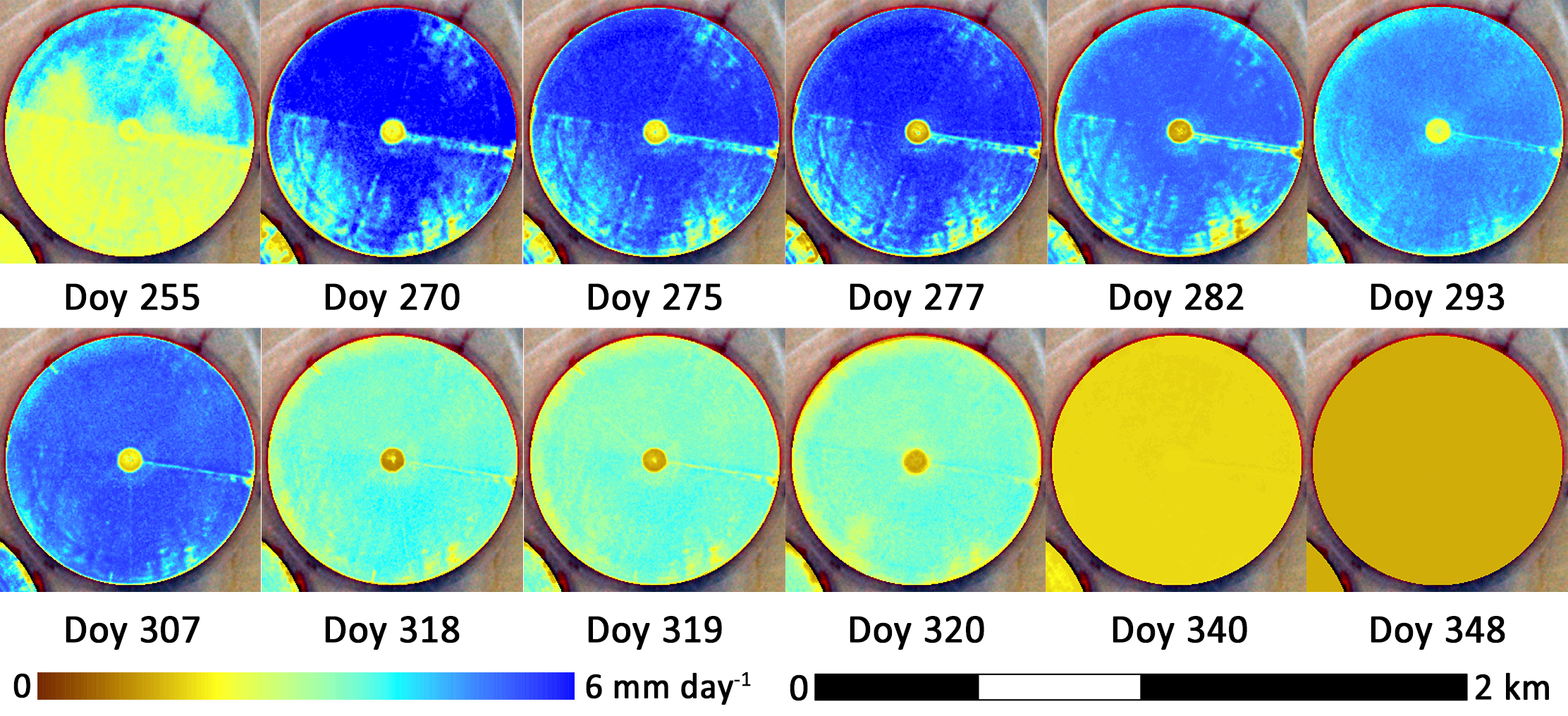
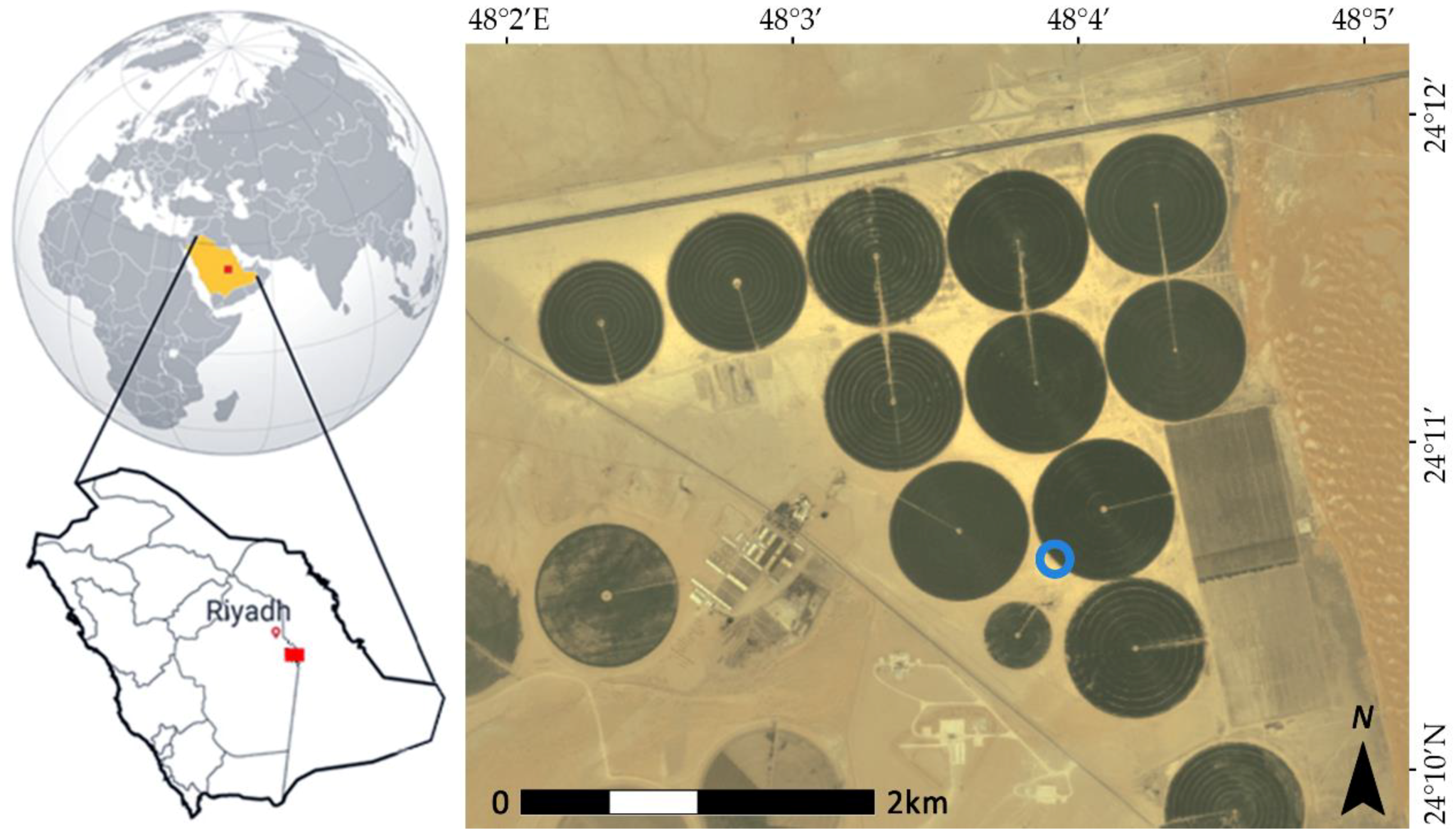
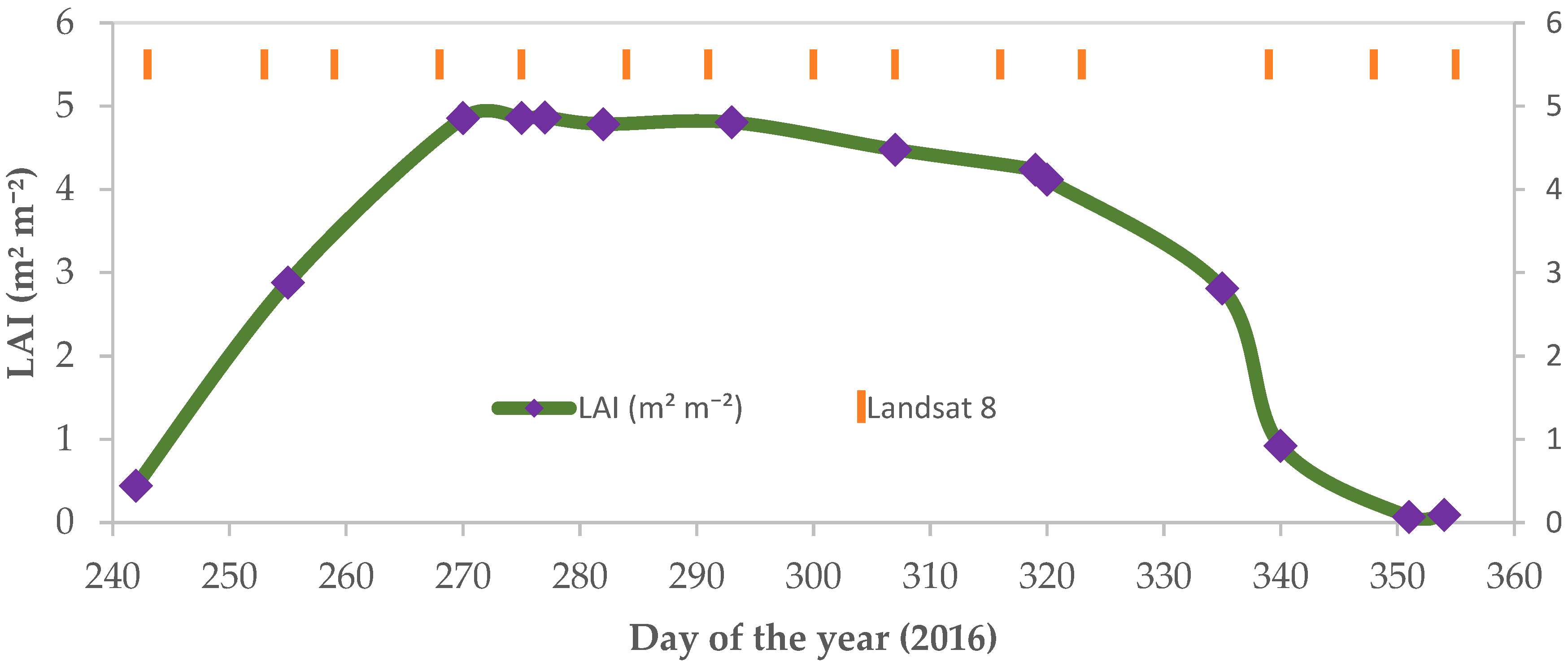
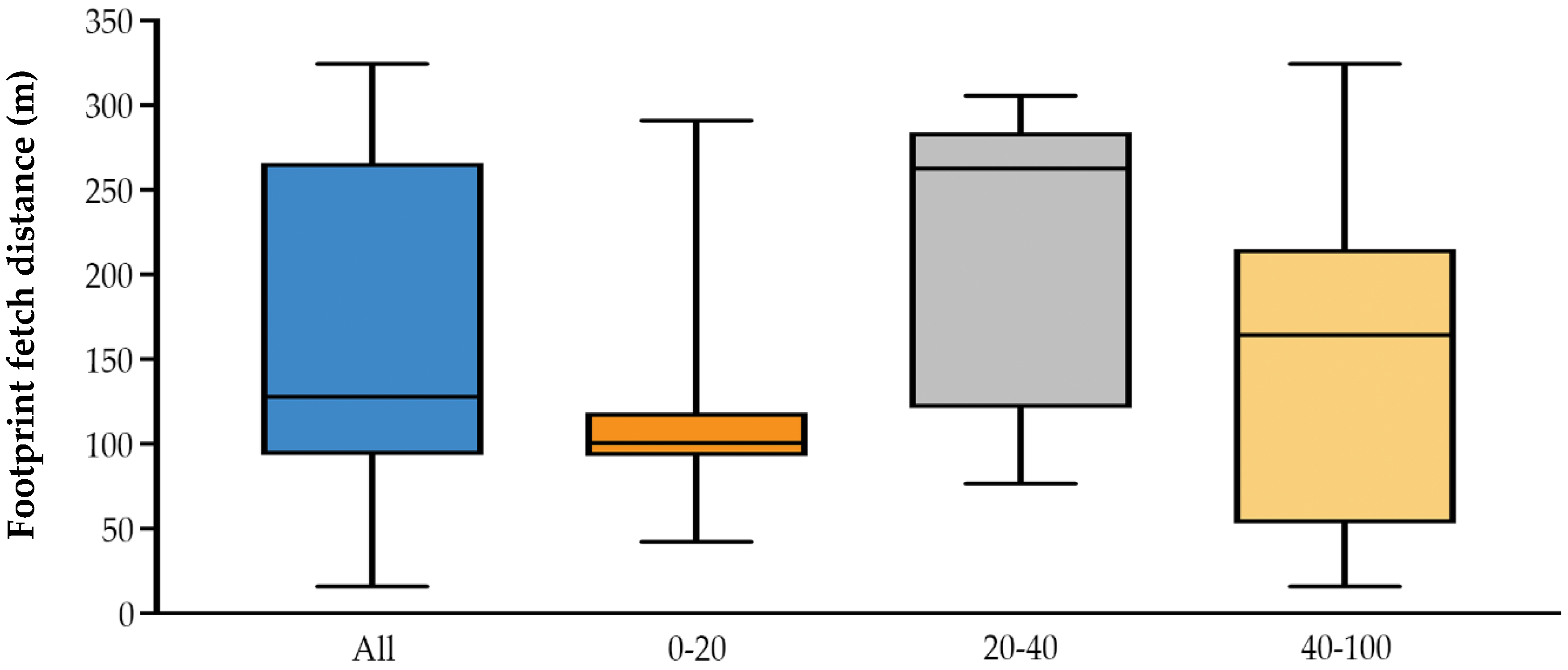
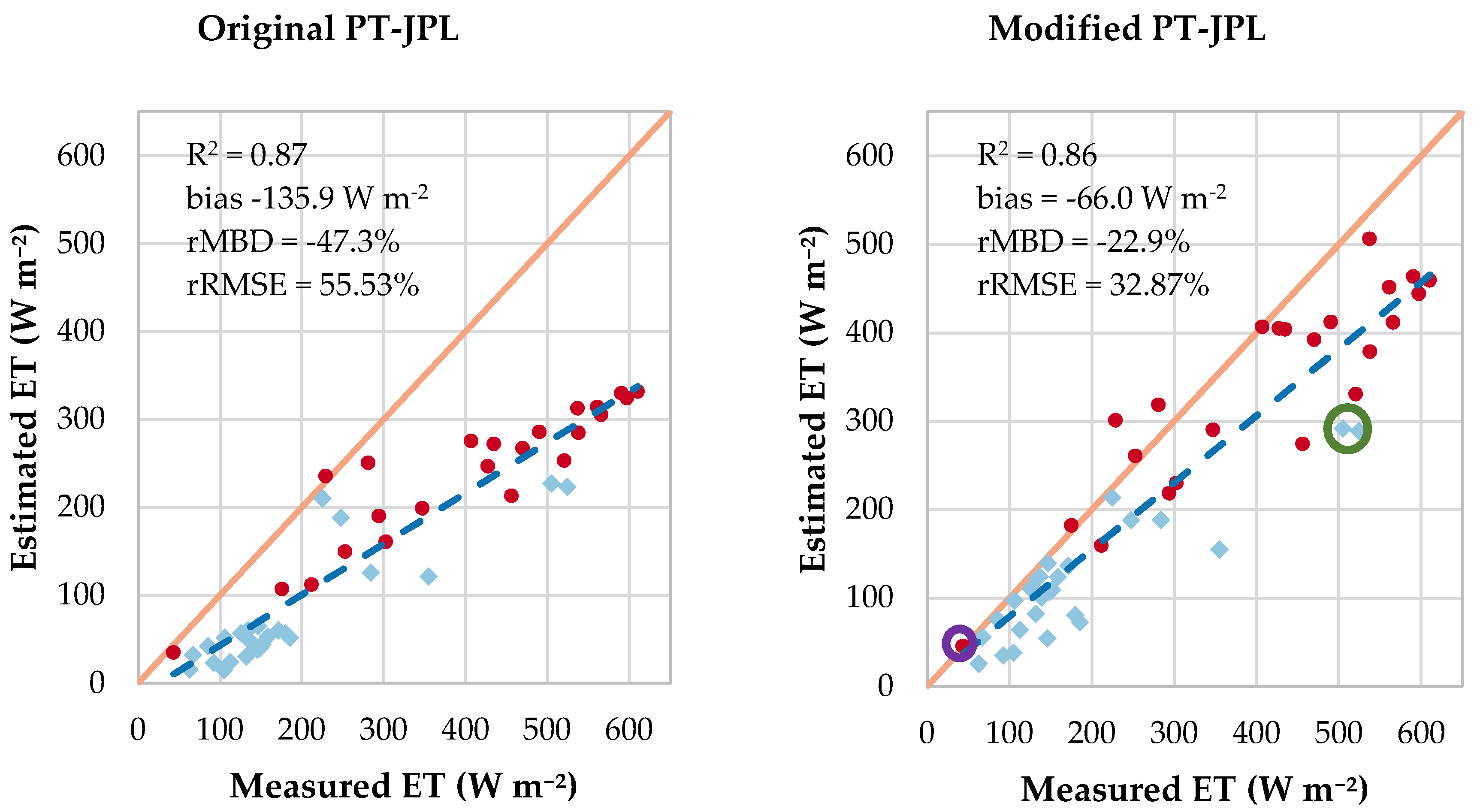
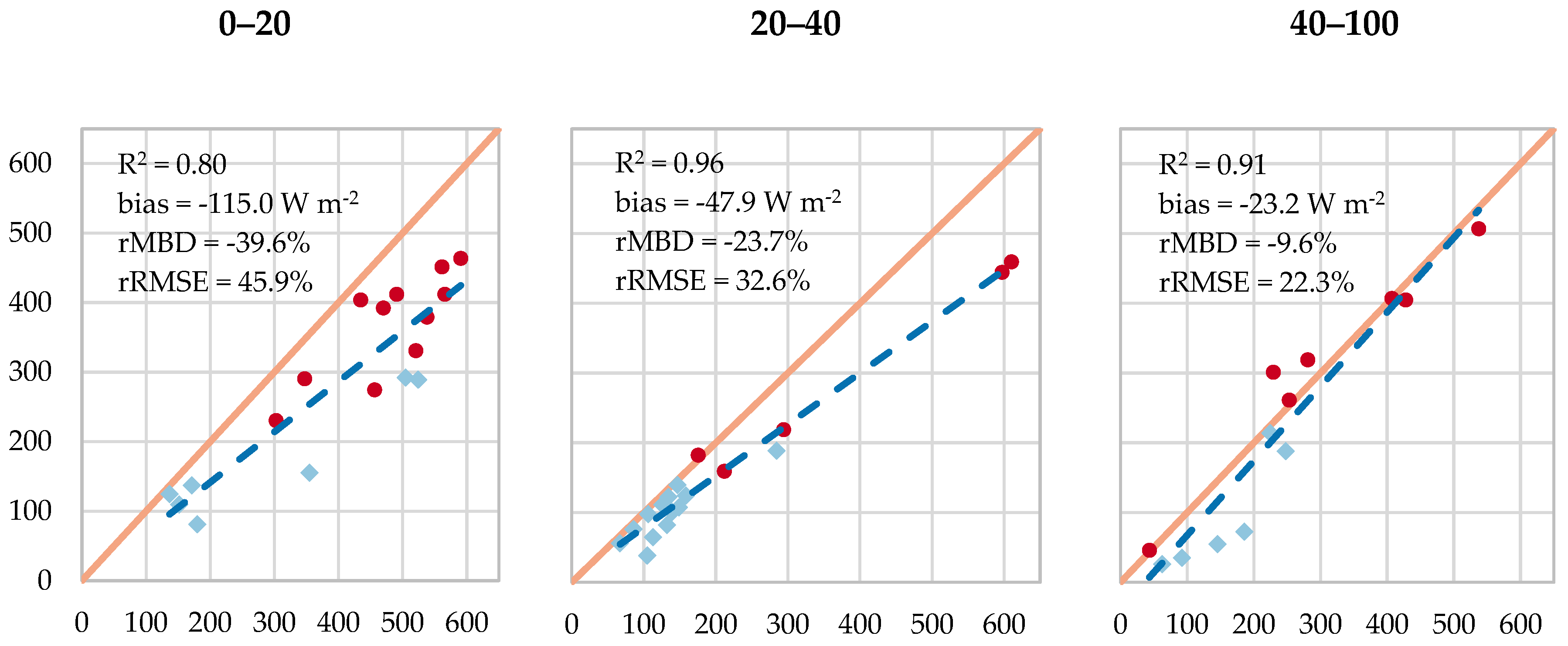
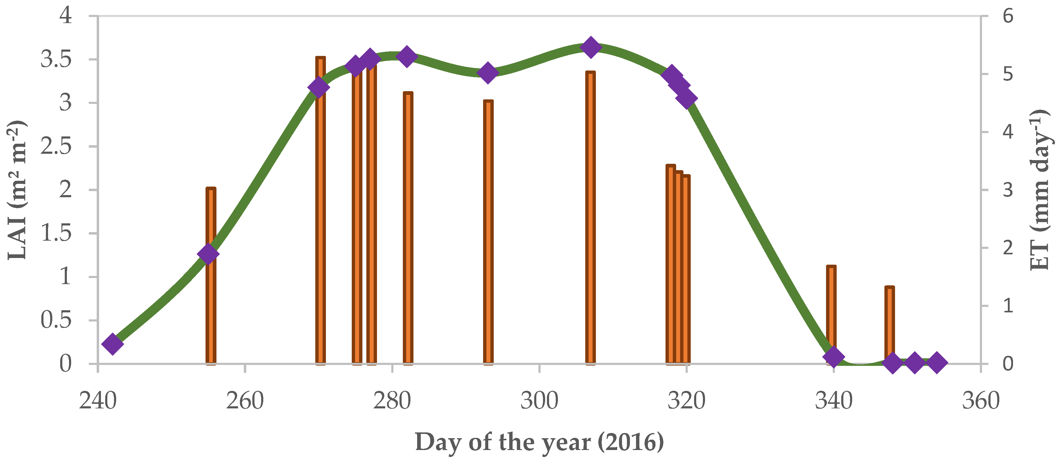
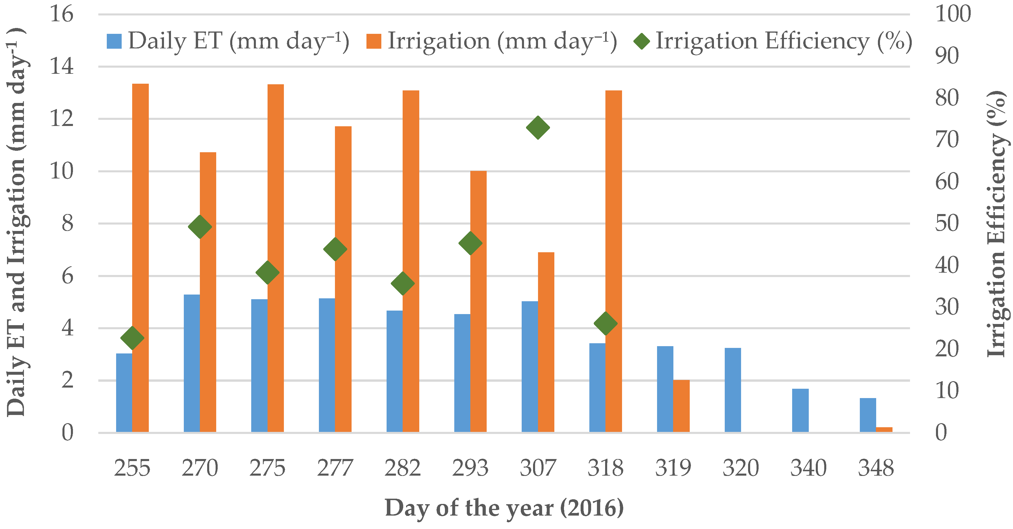
Table 1.
Statistical metrics used for model assessment. Where is the covariance between the measured values and the footprint integrated remote sensing retrievals , is the standard deviation, is the mean value of the observed values and is the number of samples.
Table 1.
Statistical metrics used for model assessment. Where is the covariance between the measured values and the footprint integrated remote sensing retrievals , is the standard deviation, is the mean value of the observed values and is the number of samples.
| Statistic | Formula | Notes |
|---|---|---|
| Coefficient of determination | Measures the percent of the variability explained by the model | |
| Bias | The mean error between the observations and the estimations | |
| Relative mean bias difference | Normalized by the mean value of the observations | |
| Root mean square error | Gives an indicator of model accuracy | |
| Relative root mean square error | Normalized by the mean value of the observations |
© 2018 by the authors. Licensee MDPI, Basel, Switzerland. This article is an open access article distributed under the terms and conditions of the Creative Commons Attribution (CC BY) license (http://creativecommons.org/licenses/by/4.0/).
Share and Cite
MDPI and ACS Style
Aragon, B.; Houborg, R.; Tu, K.; Fisher, J.B.; McCabe, M. CubeSats Enable High Spatiotemporal Retrievals of Crop-Water Use for Precision Agriculture. Remote Sens. 2018, 10, 1867. https://0-doi-org.brum.beds.ac.uk/10.3390/rs10121867
AMA Style
Aragon B, Houborg R, Tu K, Fisher JB, McCabe M. CubeSats Enable High Spatiotemporal Retrievals of Crop-Water Use for Precision Agriculture. Remote Sensing. 2018; 10(12):1867. https://0-doi-org.brum.beds.ac.uk/10.3390/rs10121867
Chicago/Turabian StyleAragon, Bruno, Rasmus Houborg, Kevin Tu, Joshua B. Fisher, and Matthew McCabe. 2018. "CubeSats Enable High Spatiotemporal Retrievals of Crop-Water Use for Precision Agriculture" Remote Sensing 10, no. 12: 1867. https://0-doi-org.brum.beds.ac.uk/10.3390/rs10121867
Note that from the first issue of 2016, this journal uses article numbers instead of page numbers. See further details here.