Article

A Random Forest-Based Approach to Map Soil Erosion Risk Distribution in Hickory Plantations in Western Zhejiang Province, China

1
State Key Laboratory of Subtropical Silviculture, Zhejiang A&F University, Hangzhou 311300, China
2
School of Environmental & Resource Sciences, Zhejiang A&F University, Hangzhou 311300, China
3
Fujian Provincial Key Laboratory for Subtropical Resources and Environment, Fujian Normal University, Fuzhou 350007, China
4
School of Geographical Sciences, Fujian Normal University, Fuzhou 350007, China
5
School of Geography and Tourism, Anhui Normal University, Wuhu 241002, China
6
Lin’An Meteorological Bureau, Hangzhou 311300, China
*
Author to whom correspondence should be addressed.
Remote Sens. 2018, 10(12), 1899; https://0-doi-org.brum.beds.ac.uk/10.3390/rs10121899
Submission received: 12 September 2018 / Revised: 13 November 2018 / Accepted: 25 November 2018 / Published: 28 November 2018
(This article belongs to the Special Issue Mass Movement and Soil Erosion Monitoring Using Remote Sensing)

Abstract

:
Increasing agroforestry areas with improper management has produced serious environmental problems, such as soil erosion. It is necessary to rapidly predict the spatial distribution of such erosion risks in a large area, but there is a lack of approaches that are suitable for mountainous regions. The objective of this research was to develop an approach that can effectively employ remotely-sensed and ancillary data, to map soil erosion risks in an agroforestry ecosystem in a mountainous region. This research employed field survey data, soil-type maps, digital elevation model data, weather station data, and Landsat imagery, for extraction of potential variables. It used the random forest approach to identify eight key variables—slope, slope of slope, normalized difference greenness index at leaf-on season, soil organic matter, fractional vegetation at leaf-on season, fractional soil at leaf-off season, precipitation in June, and percent of soil clay—for mapping soil erosion risk distribution in hickory plantations in Western Zhejiang Province, China. The results showed that an overall accuracy of 89.8% was obtained for three levels of soil erosion risk. Approximately one-fourth of hickory plantations were at high-risk, requiring the owners or decision makers to take proper measures to reduce the soil erosion problem. This research provides a new approach to predict soil erosion risk, based on the primary variables that can be extracted directly from remotely-sensed data and ancillary data. This proposed approach will be valuable for other agroforestry and plantations, such as Torreya grandis, eucalyptus, and the rubber tree, that are playing important roles in improving economic conditions for the local farmers but face soil erosion problems.

Graphical Abstract

1. Introduction

Agroforestry area has continuously expanded globally, due to the requirement of human well-being and improved standard of living. However, intensively and improperly managed agroforestry often resulted in serious soil erosion and environmental problems [1,2,3,4], and further affected sustainability of agroforestry ecosystems [5]. In general, agroforestry has some common characteristics—single tree species and simple stand structure, lack of shrubs and grass under tree canopy, and serious soil erosion problems [3,4]. Of the many agroforestry types, hickory (Carya cathayensis) was grown, originally, in mountainous regions with steep slopes and relatively poor soil conditions, but was expanded rapidly in the past three decades in subtropical regions of China, because of its high economic value for local people [6,7]. For the sake of intensive management and easy collection of hickory nuts, farmers often remove shrubs and grass, at least twice per year, in spring, before the addition of nutrients, and in early September, before the nut harvest (personal communications with farmers in Zhejiang Province during fieldwork). These hickory plantations have serious soil erosion problems because there is almost no understory, most of the year, as shown in Figure 1. The soil erosion is especially serious in the rainy season, during May and June, and in the leaf-off season from November to March/April, in the Zhejiang Province, requiring a suitable approach to quickly evaluate the soil erosion problem [5].
Soil erosion has long been recognized as a serious environmental problem and has gained increasing attention [8,9,10,11,12,13,14]. Many models [15,16,17,18,19,20,21,22,23,24,25,26,27,28,29,30,31,32], as summarized in Table S1, have been used for estimating the amount of soil erosion or evaluating the soil erosion risks. Ground covers, soil conditions, topography, climate, and human activities are major factors used in these models. Of the many models in Table S1, the Revised Universal Soil Loss Equation (RUSLE) may be the most extensively used model for soil erosion estimation in different ecosystems [8,33,34,35,36,37]. The RUSLE was initially developed for agricultural ecosystems with gentle slopes [8]. When RUSLE is used in a complex landscape, such as hilly or mountainous regions, calibration of these parameters, such as rainfall erosivity factor (R), soil erodibility factor (K), and cover management factor (C-factor) is often needed, thus, different equations for these kinds of calibrations have been proposed [10,38,39,40]. Therefore, direct application of RUSLE in forest or agroforestry ecosystems with steep slopes, is not recommended [5]. In reality, sometimes we do not need the quantitative estimation of soil erosion amounts, we just need the erosion risks and their spatial patterns [5]. Therefore, new approaches are needed to quickly map soil erosion risk distribution, especially for agroforestry, in a large area, which is valuable for owners to take proper measures to reduce soil erosion problems.
As the requirement to produce spatial distribution of soil erosion increases, remote-sensing and GIS technologies will play important roles in soil erosion estimation models. In previous studies, the C-factor in RUSLE was often calculated from remote-sensing data, such as vegetation indices [41], fractional vegetation and soil images [5,34], or the P-factor, using a land-use map classified from a remote-sensing image [42]. GIS, having the capability to provide powerful tools in storage, management, and processing of multiple data sources, plays an increasingly important role in estimation and mapping of soil erosion. For example, precipitation data are required in estimation of soil erosion, and GIS is often used to convert the point (weather station) data to surface images, through interpolation or regression approaches [10,38]. Soil attributes are also important factors required in soil erosion modeling, and GIS converts the point (soil sample) data and soil-type vector format map, to raster format data [38,42].
Since soil erosion is related to many factors, such as precipitation, topography, soil, vegetation cover, and human activities, a large number of variables can be extracted or calculated from these data sources. Thus, one critical step is to identify the key factors that are closely related to soil erosion risks. The traditional approach for selection of key variables is the stepwise regression [5], but the regression-based approach requires the assumption that the independent variables have linear correlations with the dependent variable, and the selected independent variables have no or weak correlations to each other [5]. However, this assumption may not be true for soil erosion studies. The random forest (RF) approach has the capability to provide a variable importance ranking [43] and has been extensively used for identifying key variables for land-cover classification and biomass estimation [44,45], but has not yet been used for soil erosion mapping. RF is a nonparametric algorithm based on the Classification and Regression Tree (CART) decision tree [43,46,47]. In the RF algorithm, three parameters need to be optimized—ntree, i.e., the number of regression trees (default is five hundred); mtry, i.e., the number of input variables per node (default value is the one-third of the total variables); and the node size (default is one) [48]. In general, the determination of ntree and mtry was based on the minimum of root mean squared error [49,50].
The overall goal of this research is to develop an approach suitable for mapping soil erosion risks in an agroforestry ecosystem in a mountainous region. Specifically, the objectives are to, (1) identify the key factors influencing soil erosion risk in hickory plantations; (2) develop a new approach to predict soil erosion risk in a mountainous region; and (3) produce spatial distribution maps of the predicted soil erosion risks for the local government or farmers, to take proper measures to reduce soil erosion problems. The new contribution of this research is to develop a random forest-based approach to predict soil erosion risk distribution in a mountainous region, by the effective use of remotely-sensed and ancillary data. In subtropical regions, many kinds of agroforestry or plantations, such as Torreya grandis, eucalyptus, and the rubber tree play important roles in improving economic conditions for the local farmers but face soil erosion problems. Therefore, the proposed approach for mapping soil erosion risk in hickory plantations will be valuable for other agroforestry and plantations.

2. Materials and Methods
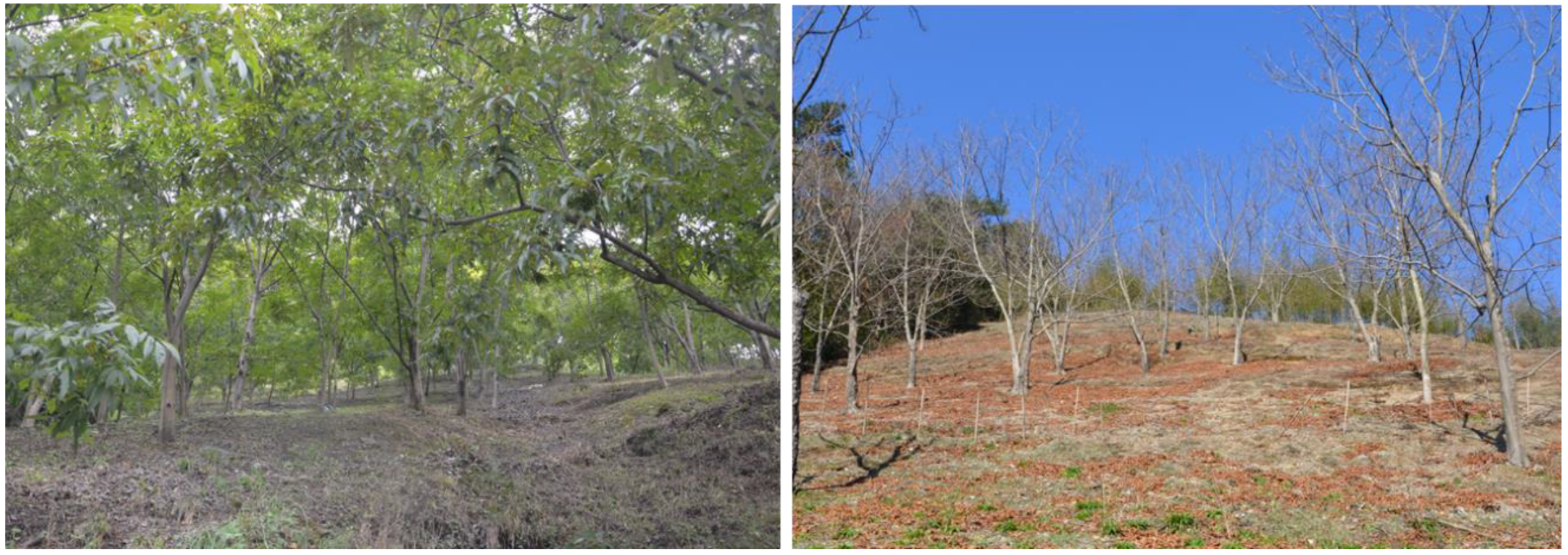
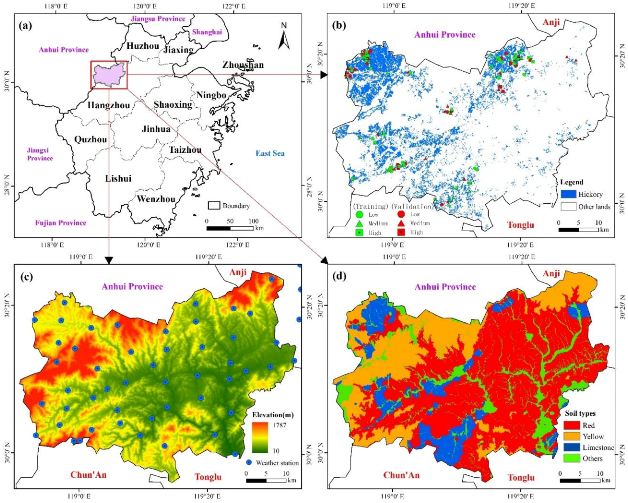
2.1. Study Area

The study area was located in the Lin’An District, Western Zhejiang Province (Figure 2), which is called the “hometown of hickory” in China [51]. This region is undulating with an elevation range of 10 m to 1787 m (average elevation of 475 m) and an average slope of 23° (see Figure 2c). The terrain has high-elevation mountainous regions in the west and low elevation with flat regions in the east. The average regional elevations are over 1000 m in the northwest and southwest, and less than 50 m in the eastern plain. This study area was scattered with plains and hills. The mountainous areas with elevations of over 500 m accounted for 33.2%, hills with elevation between 100 and 500 m accounted for 57.4%, and plains with elevation of less than 100 m accounted for 10.4% of the study areas. According to China’s soil classification system, there are 10 soil types: Red, yellow, purple, limestone, Skel, red clay, mountain meadow, Fluvo-aquic, coastal saline, and Paddy [52]. Due to the differences of soil classification systems among different countries, Table 1 provides the corresponding names which are used in the United States [53] and world reference base [54]. In our study area, the major soil types are red, yellow, and calcareous (Figure 2d).
The climate in this region is subtropical monsoon with four distinct seasons, adequate light, and abundant rainfall. According to our data, collected from sixty-seven weather stations (Figure 2c), the average annual temperature is approximately 15 °C, and annual precipitation is 1500–2000 mm. Figure 3 illustrates the average monthly precipitation values, based on the weather station data between 2002 and 2017, showing the highest monthly precipitation in June and the lowest monthly precipitation in December.
Typical forest type is the subtropical evergreen broadleaf forest. Coniferous forest, deciduous forest, and shrubs are also common [55]. In this region, the hickory plantation (Figure 2b) plays an important role in the local farmers’ economy [6,56]. The hickory plantation area increased from 113 km2 in 1983 to 320 km2 in 2014, with the production of nuts increasing from 2,300 tons to 25,000 tons, during the same period [7]. Due to the intensive and improper management of the hickory plantations, in this region, soil erosion has become a serious problem [5] that has resulted in land degradation and poor water quality.
In order to evaluate the soil erosion problem, Figure 4 illustrates the framework of predicting soil erosion risks using remote-sensing and GIS. The major steps include, (1) collection of different source data, such as soil, weather, digital elevation model (DEM), and remotely-sensed data; (2) extraction of potential variables from different datasets; (3) identification of key variables using the RF approach and developing a soil erosion risk-mapping approach; and (4) examination of the soil erosion risks for the young and mature hickory plantations.

2.2. Data Collection and Processing

Datasets used in this research (Table 2) included, (1) field survey data for determining the soil erosion risk levels, (2) Landsat images in the leaf-on and leaf-off seasons, for mapping hickory plantation distribution and for extraction of potential variables for mapping the soil erosion risk distribution, (3) weather station data, (4) soil data, and (5) DEM data. In general, the Universal Transverse Mercator (UTM) coordinate system is used in this type of research, but considering that this study crosses two UTM zones, the Albers Equal Area coordinate system with WGS 1984 datum was selected for this research.

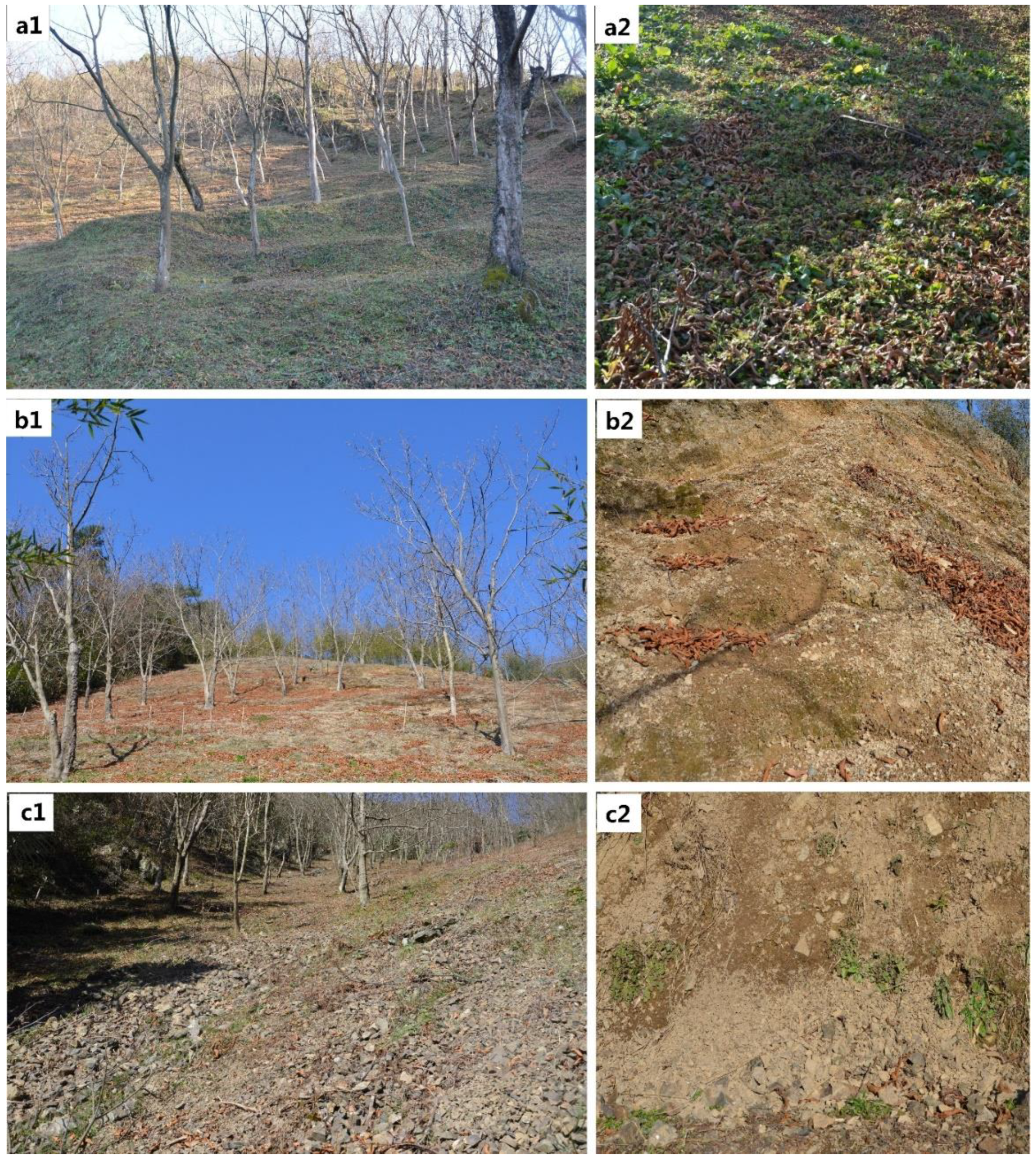
2.2.1. Field Data Collection and Determination of Soil Erosion Risk Levels

The field survey was conducted, based on Google Earth imagery and spatial distribution of hickory plantations that were produced using the Landsat images in our previous studies [51]. A global positioning system device (Global Navigation Satellite System, GNSS) was used to obtain longitude/latitude coordinates of the central point, of each sample site. During fieldwork, we recorded the surface soil erosion conditions, soil accumulation conditions in the bottom of the catchment area, slope, ground cover, etc. The slope in degree, for each visited site, was roughly recorded through visual measurement, and the exact value was then determined from the slope image calculated from the DEM data. Based on the Standards for Classification and Gradation of Soil Erosion (SL190-2007) by China’s Ministry of Water Resources [57] and our research objectives, three levels of soil erosion risks were defined in Table 3 and the photos corresponding to each level were provided in Figure 5. The soil erosion samples covered thirty-six low-level, fifty-four medium-level, and thirty-two high-level risk areas (see the sites in Figure 2b). Sixty percent (60%) of the samples were randomly selected for use as training samples, and 40% were used for validation.

2.2.2. Remote-Sensing Data Processing and Mapping of Hickory Plantations

Two Landsat 8 OLI images were atmospherically-calibrated with FLAASH (Fast Line-of-sight Atmospheric Analysis of Hypercubes) [58,59]. The C-correction approach was used for topographic correction [60], using the DEM data, with 12.5-m spatial resolution. After atmospheric and topographic correction, five spectral bands were used in this research. The blue spectral band was not used because of its serious atmospheric impacts.
Ground cover is an important factor that is directly related to soil erosion risks [61]. Vegetation indices are often used to reflect the vegetation cover. Here we used three vegetation indices—the normalized difference vegetation index (NDVI = (NIR − Red)/(NIR + Red)), the normalized difference greenness index (NDGI = (Green − Red)/(Green + Red)), and the simple ratio (SR = NIR/Red) [62]. In addition, we developed three fractional images—green vegetation, soil, and shade—from the Landsat multispectral imagery, using linear spectral mixture analysis [63], from which these three endmembers were extracted, using the image-based endmember selection approach [63]. The fractional vegetation and fractional soil images have physical meanings, representing the proportions of vegetation and soil in a unit—the cell size of the Landsat image in our study. As hickory is a deciduous tree species, the image differencing of the spectral bands, between the leaf-on and leaf-off seasons, can highlight new information about vegetation and soil features and was used in this research.
In order to examine the spatial patterns of soil erosion risks, it is necessary to accurately map agroforest types, especially hickory plantations. In this research, two Landsat OLI images, leaf-on and leaf-off, with 30-m spatial resolution, were used. Different variables, including spectral bands, vegetation indices (e.g., NDVI, NDGI, and SR), textural images using mean, standard deviation, skewness, and entropy [64], with window sizes of 3 × 3, 5 × 5, 7 × 7, 9 × 9, and 11 × 11, based on the first component (PC1) from the principal component analysis (PCA) of the multispectral images, and differences between the leaf-on and leaf-off images, were used for the land-cover classification using the RF classification approach. The use of PC1 is that it concentrates the highest information loads from the Landsat multispectral bands, as shown in Table 4 that the PC1 contained 80.8% in the leaf-on data and 82.8% in the leaf-off data. Figure 6 illustrates the color composites from the leaf-on and leaf-off seasons and the corresponding PC1 images, indicating that the hickory plantations have different spectral features, caused by seasons.
A classification system including young hickory, mature hickory, other broadleaf forests, coniferous forests, bamboo forests, shrub, agricultural lands, water, impervious surfaces, and bare lands, was selected. Training samples were selected from the field survey and Google Earth images. The classification result was then grouped into three classes—young hickory, mature hickory, and other land covers (Figure 2b). Since this research only used the classification image for analyzing soil erosion distribution in hickory plantations, a detailed description of the classification procedure is not provided here, but a similar procedure can be found in Cheng et al. [65].
Accuracy assessment is often required for understanding the quality of the classification image. In general, error matrix was developed through the use of validation samples. Overall classification accuracy was calculated from the error matrix to evaluate the overall performance, while the user’s and producer’s accuracies for specific land-cover types were calculated [66]. About forty validation samples for each land-cover class were collected independently from the field survey and the Google Earth imagery. An overall classification accuracy of 89.5% and a kappa coefficient of 0.88 were obtained. Meanwhile, the user’s and the producer’s accuracies were 95.2% and 88.9%, respectively, for young hickory, and 88.7% and 90.2%, respectively, for mature hickory.

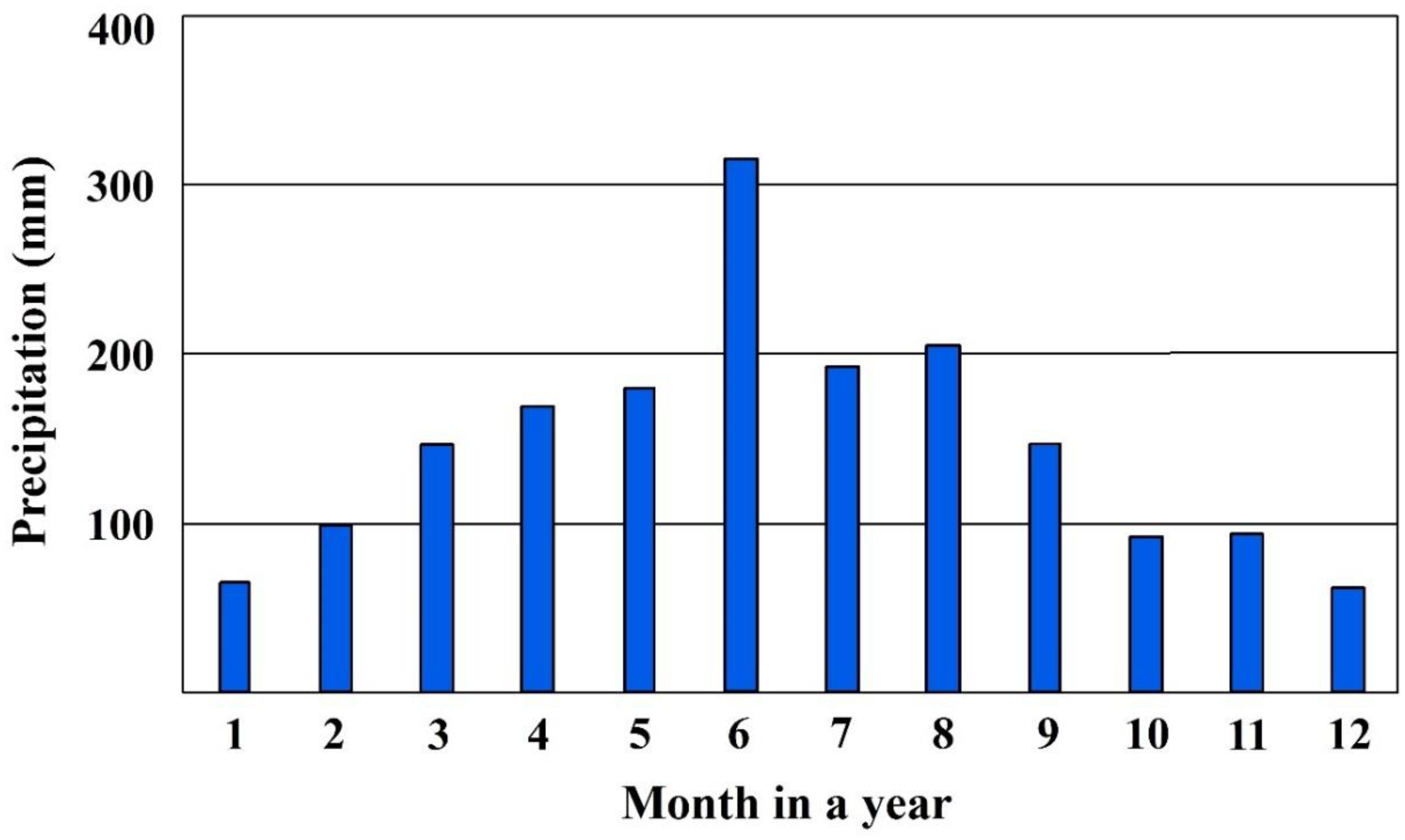
2.2.3. Collection of Precipitation Data and Development of Its Spatial Distribution

The monthly precipitation data between 2002 and 2017 were collected from sixty-seven weather stations in the study area. In order to produce a good-quality precipitation surface image, five interpolation approaches—Kriging, inverse distance weight (IDW), spline, natural neighbor, and Trend [67]—were explored, using 60% of the weather stations (i.e., 40), and their predicted spatial distributions of precipitation were validated using the remaining twenty-seven stations. The validation of these results indicated that the IDW had the smallest relative root mean squared error of 9.56%, compared to the other four approaches (i.e., 10.45% for Kriging, 14.50% for spline, 14.54% for natural neighbor, and 11.59% for Trend). In order to produce the best interpolation result, all weather stations were finally used to produce the monthly precipitation map using the IDW method. This map was resampled to a 30 m by 30 m cell size, to match the Landsat image with a 30 m spatial resolution. As precipitation is directly related to runoff, and is an important factor in soil erosion, the intensity and seasonal variation of precipitation, can affect it. Thus, more variables—annual precipitation, precipitation at leaf-on (April–October) and leaf-off (November–March) seasons, leaf-developing stage (April), flowering stage (May), and fruiting stage (June–October)—were calculated from the average monthly precipitation map.

2.2.4. Collection and Processing of Soil Data

Soil data were collected from the second soil survey in the Zhejiang Province [68]. Field survey and analysis of soil samples were two critical steps. During the field survey, 1:50,000-scale topographic maps were used to determine the collection of soil samples. Soil profiles were used to determine soil types, soil depth, and the physical and chemical properties. A soil hydrometer was used to measure the soil structure composition, such as the percentages of sand, silt, and clay. The Chemical Oxygen Demand was used to measure soil organic matter (SOM). The analysis of physical and chemical properties provided the fundamentals for the final determination of soil type classification and mapping [52]. The major attributes gleaned from the soil data included type, depth, structure (e.g., the percentages of sand, silt, and clay), and organic matter. These soil attributes, with a vector format (1:50,000), were resampled to a cell size of 30 m by 30 m, according to the maximum area allocation approach [69].

2.2.5. Extraction of Topographic Factors

Topographic factors were calculated from the advanced land observing satellite (ALOS) DEM data, with a cell size of 12.5 m by 12.5 m. The common variables included slope, aspect, and elevation. Other advanced variables were also used; for example, slope of slope (SOS) and the second derivative of surface elevation related to the horizontal surface, representing the terrain curve features [70]. According to the slope calculation theory, SOS re-calculates the slope of each point, based on the slope image from the DEM data, or the SOS = arctan (slope difference/horizontal distance). Second, surface roughness, the ratio of surface area at a specific region and its projected area, represented the fragmentation and degree of erosion [70]. Based on the slope image, surface roughness = 1/cos (slope). Third, flow accumulation and catchment area, based on DEM and precipitation data, using the ArcGIS spatial analyst and arc hydro extension, was also used [41,71]. Using precipitation data can improve the quality of the extracted flow accumulation and catchment area because the initial water value for each pixel was determined from the precipitation map. All the topographic factors, calculated from the DEM data, with a cell size of 12.5 m by 12.5 m, were resampled using the bilinear resampling technique to the cell size of a 30 m by 30 m, the same size as the Landsat imagery.

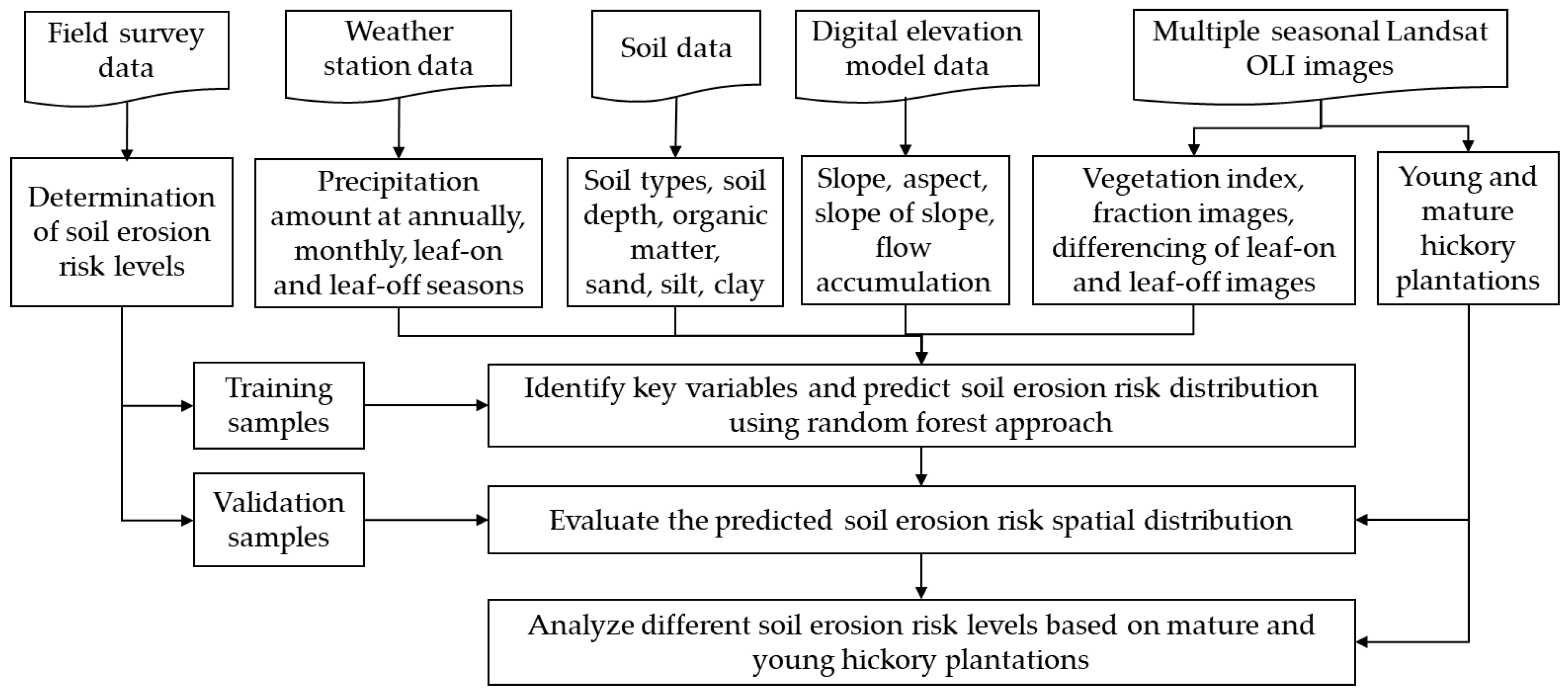
2.3. Determination of Key Variables for Mapping Soil Erosion Risk Distribution and Evaluation of Mapping Results

Many potential factors can influence soil erosion, but not all are needed for soil erosion estimation. The potential variables extracted from different sources (e.g., DEM, soil, weather stations, and remote-sensing data) are summarized in Table 5. The key is to identify the proper variables. The RF approach can provide the order of independent variable importance, related to a dependent variable, and was used here. Based on the seventy-three training samples, the RF provided the order of importance of independent variables. The backward feature elimination was further used to remove the variables that were less important but had a high correlation with another variable, so the minimum number of key variables could be identified.
After the optimized parameters were determined, the RF approach, based on these key variables was used to predict soil erosion risk distribution for the entire study area. This prediction map was evaluated using field survey data. Forty-nine validation samples, covering three levels of erosion risks, were used for evaluating the prediction map. As the prediction map is a categorical image (three risk levels), the traditional accuracy assessment approach, based on the error matrix, could be used [66]. From this error matrix, overall accuracy was calculated to indicate the overall mapping performance, while the producer’s and the user’s accuracies were calculated to show the mapping performance of the individual classes, that is, each risk level in this research.

3. Results

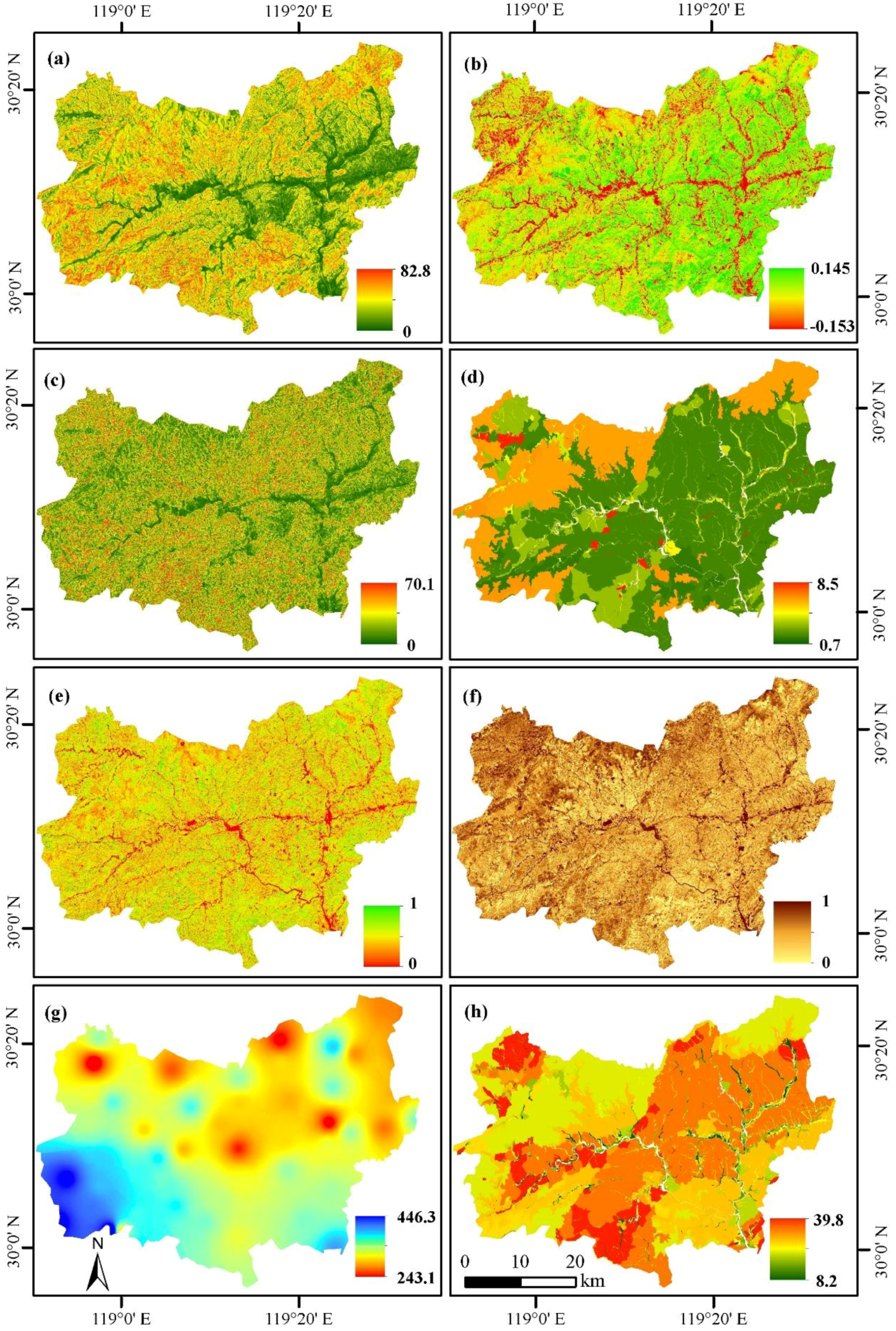
3.1. Analysis of Selected Key Variables for Mapping Soil Erosion Risk Distribution

According to the RF results, eight key variables—slope, NDGI at leaf-on season, SOS, SOM, fractional vegetation at leaf-on season, fractional soil at leaf-off season, precipitation in June (the average rainfall between 2002 and 2017), and percent of soil clay—were selected; their spatial distributions are illustrated in Figure 7. Slope and SOS were extracted from the DEM (representing the topographic condition); NDGI, fractional vegetation, and fractional soil were extracted from the Landsat multispectral imagery (representing the conditions of the vegetation cover); SOM and percent of soil clay were extracted from the soil data (representing soil features); and precipitation in June was gleaned from the interpolation of the weather station data. These key variables confirmed the complexity of soil erosion estimation that required consideration of different factors from topography, soil, vegetation cover, and precipitation [13,72]. Of the eight key variables, three were directly extracted from the multispectral imagery, implying the important role of remotely-sensed data in soil erosion risk mapping, which have not been effectively used in traditional soil erosion studies.
The roles of these key factors varied, as shown in Table 6. For example, as the risk levels increased from low to high, the values of slope, SOS, and the fractional soil in the leaf-off season, increased, implying that these factors resulted in soil erosion; in contrast, the values of NDGI at the leaf-on season, the SOM, the fractional vegetation at the leaf-on season, and percent of clay decreased, implying their roles in reducing soil erosion. In a relatively small region, precipitations can be similar but are directly related to soil erosion. The average precipitation in June was selected as a key variable, probably because the highest rainfall of the year occurs during that month, resulting in high erosion risk.
The importance ranking in Table 6 indicates that the topographic factors (i.e., slope (1st) and SOS (3rd)) play the most important roles, resulting in serious soil erosion problems. While the green vegetation cover (NDGI in the leaf-on season (2nd) and the fractional vegetation in the leaf-on season (5th)), and soil exposure (fractional soil in leaf-off season (6th)), indicate the necessity of maintaining a highly dense vegetation cover and minimizing the soil exposure, to reduce soil erosion risk. The values of each factor, with erosion risk levels (Table 6), may provide some important guidelines for the hickory plantation owners to better manage them. For example, the risk levels increase as slope and SOS values increase, implying that the mountainous regions, with slopes greater than 25°, should be managed with caution. The decrease of NDGI and vegetation in the leaf-on season and increase of the fractional soil in leaf-off season, associated with higher risk levels, indicate the importance of keeping dense vegetation cover to reduce the soil erosion problems. While the decreases in SOM and clay percentages, from low to high risk levels, imply the role of the soil structure in reducing soil erosion risks. Table 6 implies that planting agroforest plantations in gentle slope regions, while keeping dense vegetation cover and more SOM and clay components in soil, can reduce soil erosion risk.

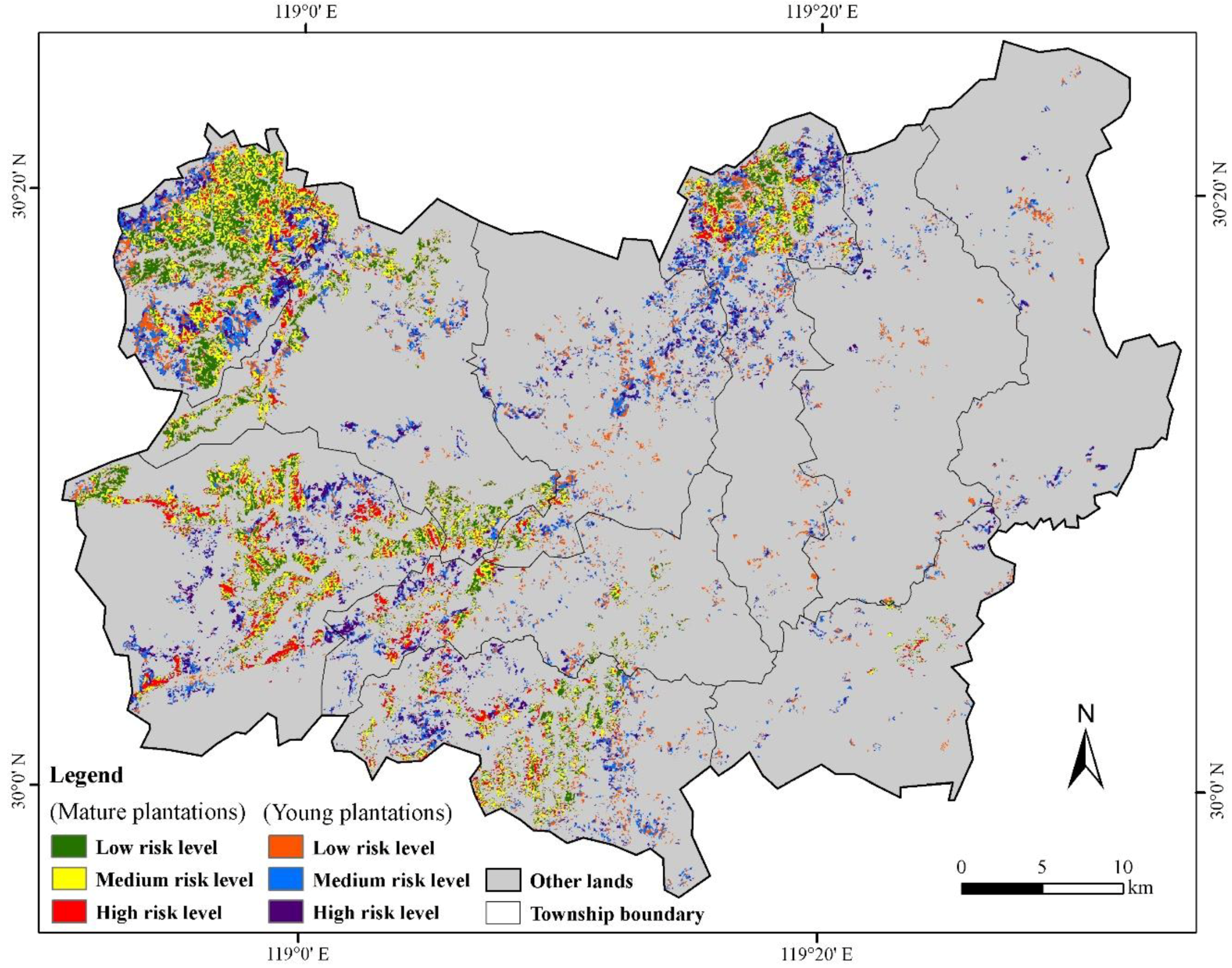
3.2. Analysis of Soil Erosion Risk Mapping Results

The accuracy assessment result (Table 7) indicates that an overall accuracy of 89.8% was obtained, with producer’s accuracy of 84.6–95.2% and user’s accuracy of 83.3–100%, for three risk levels. The high accuracy indicates that the RF-based approach, using the selected key variables, can successfully predict soil erosion risk distribution in a large area. The spatial patterns of three erosion risk levels in Figure 8 shows different levels of erosion risk dispersed in different regions of the hickory plantations. The high erosion risk level is more prevalent in the southwest part of the study area.
The statistical results in Table 8 indicate that, of the total hickory plantation areas of 325.5 km2, about one-fourth of the area is at a high-risk level, requiring their owners to take suitable measures to reduce the soil erosion problem. Although both mature and young hickory plantations have common erosion problems, a larger proportion of young hickory plantations are at high risk. If no remedies are applied in the near future, the high-risk plantations may not be sustainable.

4. Discussion

4.1. The Roles of Remote-Sensing Data in Soil Erosion Risk Mapping

Remote sensing can accurately reflect land surface information, at the time-point when a satellite or plane passes over. However, remote-sensing data itself cannot directly provide meaningful information for soil erosion, which may be why remote-sensing data has not been used extensively for soil erosion estimation or mapping. One important role of remote-sensing data may be the calculation of the C-factor, because the data can provide vegetation cover information that is closely-related to the C-factor. The C-factor is usually calculated using individual soil loss ratio values and the factors of rainfall and runoff erosivity [8], or a combination of an individual C-factor, from empirical models, and a classified remote-sensing image [73]. Some previous research has used the vegetation index [41] or fractional vegetation and soil images [5,34] to calculate the C-factor. However, no accuracy assessment was conducted because no ground truth or reference data were available for evaluation of this calculation result. This research also confirmed the important role of using remote-sensing-derived variables for soil erosion risk mapping. Three variables—NDGI at leaf-on season, fractional vegetation at leaf-on season, and fractional soil at leaf-off season—were identified in this research as key variables for soil erosion risk mapping. These variables can be extracted directly from the Landsat multispectral images, implying that they play an important role in accurately mapping the spatial distribution of soil erosion risks. Even as more types of remote-sensing data with very different spatial resolutions (e.g., from 0.5 m to 1 km) become available, the effective process of extracting the best variables for the soil erosion risk mapping is still poorly understood. This research indicates that for the hickory plantations—a deciduous tree species—use of the leaf-on and leaf-off seasonal images is needed. However, more research is needed to identify proper variables from remotely-sensed data for other tree species, such as evergreen broadleaf or needle-leaf forest types.

4.2. The Roles of GIS in Soil Erosion Risk Mapping

GIS has long been regarded as a powerful tool for storage, management, organization, and processing of different kinds of data sources [74]. It is especially valuable for soil erosion studies because it requires a combination of different data sources, such as DEM, soil, climate, and remote-sensing–derived products. These data sources often have various formats, qualities, and spatial resolutions that require GIS to handle them. Previous research has extensively used GIS technologies to solve environmental problems [74]; for instance, SOM was mapped using a geographically weighted regression approach, based on the SOM sample plots, the DEM, and remote-sensing data [3]. This research also confirmed the value and necessity of using GIS in soil erosion risk mapping. For example, this research used GIS technologies to calculate slope, SOS, surface roughness, and flow accumulation from DEM data, and converted the monthly precipitation from weather stations to surface image, through the IDW interpolation approach.
Compared to remote-sensing data with raster format and high spatial resolution, most GIS data, such as soil data in vector format and precipitation data in point format, from weather stations, have relatively coarse spatial resolutions and poor data quality, and requires conversion of these data into raster format data with the same cell size as the selected remote-sensing data. Some advanced techniques are needed to improve the data quality [3]. For example, direct interpolation of the SOM data, based on sample plots, yields a poor SOM distribution result, while the use of a geographically weighted regression approach to combine DEM and remote-sensing data, considerably improved the spatial patterns of the predicted SOM distribution [3]. A similar situation occurred in this research with the precipitation image. Currently, we use the IDW to interpolate the monthly precipitation weather station data into a surface image, but the bullseye effect was obvious, as shown in Figure 7g. In the mountainous regions, topography may considerably influence the rainfall amounts and spatial patterns in a large area. It will be necessary to combine the topographic information in the future for predicting the precipitation spatial distribution.
Data quality and spatial resolution are important factors influencing soil erosion mapping performance. In particular, the quality of DEM data was critical for calculation of slope and SOS that were used in this research. This is because the current DEM data from Shuttle Radar Topography Mission (SRTM), Advanced Spaceborne Thermal Emission and Reflection Radiometer (ASTER), or ALOS are more similar to the DSM (digital surface model) than to the DEM, thus, it may affect the accuracy of calculation of the slope and the SOS. In reality, DEM is a difference of the DSM and the object height image. In a mountainous region, the tree height value is much smaller, compared to the elevation value, thus DSM is often used as DEM, by ignoring the tree height. If lidar data could have been obtained in the given study, the lidar-derived DEM data should be used. In addition to the DEM data, another important data source is soil, for which SOM and clay percentages were used, in this research. Obtaining good-quality soil data is especially a challenge. The soil data were often assumed constant, but, in reality, the soil structure and nutrient composition could be changed due to human activities (e.g., addition of fertilizers) and soil erosion. More research is needed to update the soil data in a timely manner, using the GIS-based modeling approach, based on soil sample plots, and remote-sensing and ancillary data [3].

4.3. The Approach to Identify Key Variables for Mapping Soil Erosion Risk Distribution

Different soil erosion estimation models (see Table S1) have their own requirements for data sources, thus estimation results could be hugely different. Cautions should be taken when a model is used in mountainous regions because of the very complex landscape, compared to agricultural lands. In many soil erosion applications, the exact soil erosion amount may not be required, and people may just need to know the spatial distribution of different erosion risk levels, so they can take proper measures to reduce the soil erosion problems in a large area. This research used an RF-based approach to identify key variables for mapping soil erosion risk distribution. The selected eight variables are from DEM, soil, precipitation, and remote-sensing data (vegetation cover information), implying that similar data sources are required for soil erosion studies. However, comparing the models in Table S1, the advantages of this RF-based approach for mapping soil erosion risk distribution are, (1) the use of primary variables that can be directly extracted from different data sources without calibration; (2) the important role of the leaf-on and the leaf-off Landsat multispectral images in producing the vegetation- and soil-related variables, with high spatial resolution images, compared to the GIS data (e.g., soil, precipitation); and (3) the potential applications to other agroforest systems, such as eucalyptus, Torreya grandis, and plantations in subtropical regions. However, cautions should be taken that this research is only for hickory plantations, a deciduous tree species; the selected key variables suitable for the hickory plantations may be not the best variables for other plantations. Therefore, more research is needed to identify the best key variables for other forest types, under different topographic conditions.

5. Conclusions

This research selected a typical agroforestry region in a subtropical forest ecosystem to examine the remote-sensing and GIS–based approach to map soil erosion risk distribution. This research used the RF approach to identify eight primary variables—slope, SOS, NDGI at the leaf-on season, fractional vegetation at the leaf-on season, fractional soil at the leaf-off season, SOM, clay, and average precipitation in June—that could be directly extracted from the DEM, the Landsat multispectral imagery, soil, and the weather station data. The results showed that 25.7%, 41.8%, and 32.5% of the hickory plantations in this study area were at high, medium, and low erosion risk levels, respectively, indicating serious soil erosion problems and requiring urgent measures to maintain their sustainability. This research indicates the important role of remote-sensing data in mapping soil erosion risk distribution and provides a new approach to rapidly predict soil erosion risk distribution, using remote-sensing and GIS technologies. The major advantage of this RF-based soil erosion risk-mapping approach is that the selected variables can be directly extracted from remotely-sensed data, DEM, and soil data, without calibration of the empirical models. The proposed approach may be applied to other agroforestry or plantations, but cautions should be taken in other environments. More research is needed to identify the key variables for other forest types, especially the evergreen forest types, under complex forest ecosystems.

Supplementary Materials

The following are available online at https://0-www-mdpi-com.brum.beds.ac.uk/2072-4292/10/12/1899/s1. Table S1: summary of major soil erosion estimation models.

Author Contributions

Conceptualization, D.L. and J.H.; methodology, D.L., Z.C. and G.L.; software, Z.C.; validation, Z.C., G.L. and N.S.; formal analysis, Z.C. and G.L.; investigation, Z.C. and N.S.; resources, Z.C., J.Z. and S.L.; data curation, Z.C., J.Z. and S.L.; writing original draft, Z.C. and D.L.; review and editing, D.L. and G.L.; visualization, D.L.; supervision, D.L.; project administration, D.L.; funding acquisition, D.L. and J.H.

Funding

This research was financially supported by Zhejiang Provincial Natural Science Foundation (LZ15C160001), the Zhejiang A&F University’s Research and Development Fund (2013FR052), and the Science and Technology Innovation Program for Undergraduates in Zhejiang Province (2018R412038).

Acknowledgments

The authors would like to thank Dengqiu Li, Longwei Li, Yajie Wang, and Wei Lu for their helps in the fieldwork, and thank three anonymous reviewers for their constructive comments and suggestions.

Conflicts of Interest

The authors declare no conflict of interest.

References

  1. Gusarov, A.V.; Golosov, V.N.; Sharifullin, A.G. Contribution of climate and land cover changes to reduction in soil erosion rates within small cultivated catchments in the eastern part of the Russian plain during the last 60 years. Environ. Res. 2018, 167, 21–33. [Google Scholar] [CrossRef] [PubMed]
  2. Kouli, M.; Soupios, P.; Vallianatos, F. Soil erosion prediction using the revised universal soil loss equation (RUSLE) in a GIS framework, Chania, Northwestern Crete, Greece. Environ. Geol. 2008, 57, 483–497. [Google Scholar] [CrossRef]
  3. Lu, W.; Lu, D.; Wang, G.; Wu, J.; Huang, J.; Li, G. Examining soil organic carbon distribution and dynamic change in a hickory plantation region with Landsat and ancillary data. Catena 2018, 165, 576–589. [Google Scholar] [CrossRef]
  4. Wang, Y.; Lu, D. Mapping Torreya grandis spatial distribution using high spatial resolution satellite imagery with the expert rules-based approach. Remote Sens. 2017, 9, 564. [Google Scholar] [CrossRef]
  5. Huang, J.; Lu, D.; Li, J.; Wu, J.; Chen, S.; Zhao, W.; Ge, H.; Huang, X.; Yan, X. Integration of remote sensing and GIS for evaluating soil erosion risk in northwestern Zhejiang, China. Photogramm. Eng. Remote Sens. 2012, 78, 935–946. [Google Scholar] [CrossRef]
  6. Zhang, R.; Peng, F.; Li, Y. Pecan production in China. Sci. Hortic. 2015, 197, 719–727. [Google Scholar] [CrossRef]
  7. Ding, L.; Zhong, Y. Lin’an hickory. China Qual. Stand. Rev. 2014, 17, 66–68. [Google Scholar]
  8. Renard, K.G.; Foster, G.R.; Weesies, G.A.; McCool, D.K.; Yoder, D.C. Predicting Soil Erosion by Water: A Guide to Conservation Planning With the Revised Universal Soil Loss Equation (Rusle); Agricultural Handbook, Number 703; US Department of Agriculture: Washington, DC, USA, 1997; p. 404.
  9. Lu, D.; Batistella, M.; Mausel, P.; Moran, E. Mapping and monitoring land degradation risks in the western Brazilian Amazon using multitemporal Landsat TM/ETM+ images. Land Degrad. Dev. 2007, 18, 41–54. [Google Scholar] [CrossRef]
  10. Wang, G.; Wente, S.; Gertner, G.Z.; Anderson, A. Improvement in mapping vegetation cover factor for the universal soil loss equation by geostatistical methods with Landsat Thametic Mapper images. Int. J. Remote Sens. 2002, 23, 3649–3667. [Google Scholar] [CrossRef]
  11. Wang, G.; Gertner, G.; Anderson, A.B.; Howard, H.; Gebhart, D.; Althoff, D.; Davis, T.; Woodford, P. Spatial variability and temporal dynamics analysis of soil erosion due to military land use activities: Uncertainty and implications for land management. Land Degrad. Dev. 2007, 18, 519–542. [Google Scholar] [CrossRef]
  12. Wang, G.; Gertner, G.; Anderson, A.B. Efficiencies of remotely sensed data and sensitivity of grid spacing in sampling and mapping a soil erosion relevant cover factor by cokriging. Int. J. Remote Sens. 2009, 30, 4457–4477. [Google Scholar] [CrossRef]
  13. Albaradeyia, I.; Hani, A.; Shahrour, I. WEPP and ANN models for simulating soil loss and runoff in a semi-arid mediterranean region. Environ. Monit. Assess. 2011, 180, 537–556. [Google Scholar] [CrossRef] [PubMed]
  14. Sinha, N.; Deb, D.; Pathak, K. Development of a mining landscape and assessment of its soil erosion potential using GIS. Eng. Geol. 2017, 216, 1–12. [Google Scholar] [CrossRef]
  15. Wischmeier, W.H.; Smith, D.D. Predicting Rainfall Erosion Losses: A Guide to Conservation Planning; Agricultural Handbook, Number 537; US Department of Agriculture: Washington, DC, USA, 1978; p. 163.
  16. Williams, J.R.; Berndt, H.D. Sediment yield prediction based on watershed hydrology. Trans. Am. Soc. Agric. Eng. 1977, 20, 1100–1104. [Google Scholar] [CrossRef]
  17. Nearing, M.A.; Foster, G.R.; Lane, L.J.; Finkner, S.C. A process-based soil erosion model for USDA-water erosion prediction project technology. Trans. ASAE 1989, 32, 1587–1593. [Google Scholar] [CrossRef]
  18. Arnold, J.G.; Srinivasan, R.; Muttiah, R.S.; Williams, J.R. Large area hydrologic modeling and assessment: Part I: Model development. J. Am. Water Resour. Assoc. 1998, 34, 73–89. [Google Scholar] [CrossRef]
  19. Young, R.A.; Onstad, C.A.; Bosch, D.D.; Anderson, W.P. AGNPS: A nonpoint-source pollution model for evaluating agricultural watersheds. J. Soil Water Conserv. 1989, 44, 168–173. [Google Scholar]
  20. Kliment, Z.; Kadle, J.; Langhammer, J. Evaluation of suspended load changes using ANN AGNPS and SWAT semi-empirical erosion models. Catena 2008, 97, 286–299. [Google Scholar] [CrossRef]
  21. Walling, E.; He, Q.; Whelan, P.A. Using 137Cs measurements to validate the application of the AGNPS and ANSWERS erosion and sediment yield models in two small Devon catchments. Soil Tillage Res. 2003, 69, 27–43. [Google Scholar] [CrossRef]
  22. Recolainen, S.; Posch, M. Adapting the CREAMS model for Finnish conditions. Nord. Hydrol. 1993, 24, 309–322. [Google Scholar] [CrossRef]
  23. Morgan, R.P.C.; Quinton, J.N.; Smith, R.E.; Govers, G.; Poesen, J.W.A.; Auerswald, K.; Chisci, G.; Torri, D.; Styczen, M.E. The European soil erosion model (EUROSEM): A dynamic approach for predicting sediment transport from fields and small catchments. Earth Surf. Process. Landf. 1998, 23, 527–544. [Google Scholar] [CrossRef]
  24. Kirkby, M.J.; Irvine, B.J.; Jones, R.J.A.; Govers, G. The PESERA coarse scale erosion model for Europe. I.—Model rationale and implementation. Eur. J. Soil Sci. 2008, 59, 1293–1306. [Google Scholar] [CrossRef] [Green Version]
  25. Udayakumara, E.P.N.; Shrestha, R.P.; Samarakoon, L.; Schmidt-Vogt, D. People’s perception and socioeconomic determinants of soil erosion: A case study of Samanalawewa watershed, Sri Lanka. Int. J. Sediment Res. 2010, 25, 323–339. [Google Scholar] [CrossRef]
  26. Shi, Z.; Ai, L.; Fang, N.; Zhu, H. Modeling the impacts of integrated small watershed management on soil erosion and sediment delivery: A case study in the Three Gorges Area, China. J. Hydrol. 2012, 438, 156–167. [Google Scholar] [CrossRef]
  27. Routschek, A.; Schmidt, J.; Kreienkamp, F. Impact of climate change on soil erosion: A high-resolution projection on catchment scale until 2100 in Saxony/Germany. Catena 2014, 121, 99–109. [Google Scholar] [CrossRef]
  28. Ji, U.; Velleux, M.; Julien, P.Y.; Hwang, M. Risk assessment of watershed erosion at Naesung Stream, South Korea. J. Environ. Manag. 2014, 136, 16–26. [Google Scholar] [CrossRef] [PubMed]
  29. Fu, G.; Chen, S.; McCool, D.K. Modeling the impacts of no-till practice on soil erosion and sediment yield with RUSLE, SEDD, and ArcView GIS. Soil Tillage Res. 2006, 85, 38–49. [Google Scholar] [CrossRef]
  30. Wu, Q.; Wang, M. A framework for risk assessment on soil erosion by water using an integrated and systematic approach. J. Hydrol. 2007, 337, 11–21. [Google Scholar] [CrossRef]
  31. Zhang, X.; Wu, B.; Ling, F.; Zeng, Y.; Yan, N.; Yuan, C. Identification of priority areas for controlling soil erosion. Catena 2010, 83, 76–85. [Google Scholar] [CrossRef]
  32. Vijith, H.; Suma, M.; Rekha, V.B.; Shiju, C.; Rejith, P.J. An assessment of soil erosion probability and erosion rate in a tropical mountainous watershed using remote sensing and GIS. Arab. J. Geosci. 2011, 5, 797–804. [Google Scholar] [CrossRef]
  33. Angima, S.D.; Stott, D.E.; Oneill, M.K.; Ong, C.K.; Weesies, G.A. Soil erosion prediction using RUSLE for central Kenyan highland conditions. Agric. Ecosyst. Environ. 2003, 97, 295–308. [Google Scholar] [CrossRef]
  34. Lu, D.; Li, G.; Valladares, G.S.; Batistella, M. Mapping soil erosion risk in Rondônia, Brazilian Amazonia: Using RUSLE, remote sensing and GIS. Land Degrad. Dev. 2004, 15, 499–512. [Google Scholar] [CrossRef] [Green Version]
  35. Park, S.; Oh, C.; Jeon, S.; Jung, H.; Choi, C. Soil erosion risk in Korean watersheds, assessed using the revised universal soil loss equation. J. Hydrol. 2011, 399, 263–273. [Google Scholar] [CrossRef]
  36. Thomas, J.; Joseph, S.; Thrivikramji, K.P. Assessment of soil erosion in a tropical mountain river basin of the southern Western Ghats, India using RUSLE and GIS. Geosci. Front. 2018, 9, 893–906. [Google Scholar] [CrossRef]
  37. Conforti, M.; Buttafuoco, G. Assessing space-time variations of denudation processes and related soil loss from 1955 to 2016 in southern Italy (Calabria region). Environ. Earth Sci. 2017, 76, 457. [Google Scholar] [CrossRef]
  38. Ferreira, V.; Panagopoulos, T.; Cakula, A.; Andrade, R.; Arvela, A. Predicting soil erosion after land use changes for irrigating agriculture in a large reservoir of southern Portugal. Agric. Agric. Sci. Procedia 2015, 4, 40–49. [Google Scholar] [CrossRef]
  39. Brhane, G.; Mekonen, K. Estimating soil loss using Universal Soil Loss Equation (USLE) for soil conservation planning at Medego watershed, Northern Ethiopia. J. Am. Sci. 2009, 5, 58–69. [Google Scholar]
  40. Pei, T.; Qin, C.; Zhu, A.; Yang, L.; Luo, M.; Li, B.; Zhou, C. Mapping soil organic matter using the topographic wetness index: A comparative study based on different flow-direction algorithms and kriging methods. Ecol. Indic. 2010, 10, 610–619. [Google Scholar] [CrossRef]
  41. Prasannakumar, V.; Vijith, H.; Abinod, S.; Geetha, N. Estimation of soil erosion risk within a small mountainous sub-watershed in Kerala, India, using revised universal soil loss equation (RUSLE) and geo-information technology. Geosci. Front. 2012, 3, 209–215. [Google Scholar] [CrossRef]
  42. Jiang, Z.; Su, S.; Jing, C.; Lin, S.; Fei, X.; Wu, J. Spatiotemporal dynamics of soil erosion risk for Anji county, China. Stoch. Environ. Res. Risk Assess. 2012, 26, 751–763. [Google Scholar] [CrossRef]
  43. Breiman, L. Random forests. Mach. Learn. 2001, 45, 5–32. [Google Scholar] [CrossRef]
  44. Lu, D.; Chen, Q.; Wang, G.; Liu, L.; Li, G.; Moran, E. A survey of remote sensing-based aboveground biomass estimation methods in forest ecosystems. Int. J. Digit. Earth 2016, 9, 63–105. [Google Scholar] [CrossRef]
  45. Gao, Y.; Lu, D.; Li, G.; Wang, G.; Chen, Q.; Liu, L.; Li, D. Comparative analysis of modeling algorithms for forest aboveground biomass estimation in a subtropical region. Remote Sens. 2018, 10, 627. [Google Scholar] [CrossRef]
  46. Clark, M.L.; Roberts, D.A. Species-level differences in hyperspectral metrics among tropical rainforest trees as determined by a tree-based classifier. Remote Sens. 2012, 4, 1820–1855. [Google Scholar] [CrossRef]
  47. Rodriguez-Galiano, V.F.; Ghimire, B.; Rogan, J.; Chica-Olmo, M.; Rigol-Sanchez, J.P. An assessment of the effectiveness of a random forest classifier for land-cover classification. ISPRS J. Photogramm. Remote Sens. 2012, 67, 93–104. [Google Scholar] [CrossRef]
  48. Liaw, A.; Wiener, M. Classification and regression by random forest. R News 2002, 2, 18–22. [Google Scholar]
  49. Mutanga, O.; Adam, E.; Cho, M.A. High density biomass estimation for wetland vegetation using Worldview-2 imagery and random forest regression algorithm. Int. J. Appl. Earth Obs. Geoinf. 2012, 18, 399–406. [Google Scholar] [CrossRef]
  50. Vincenzi, S.; Zucchetta, M.; Franzoi, P.; Pellizzato, M.; Pranovi, F.; De Leo, G.A.; Torricelli, P. Application of a random forest algorithm to predict spatial distribution of the potential yield of Ruditapes Philippinarum in the Venice Lagoon, Italy. Ecol. Model. 2011, 222, 1471–1478. [Google Scholar] [CrossRef]
  51. Xi, Z.; Lu, D.; Liu, L.; Ge, H. Detection of drought-induced hickory disturbances in western Lin An county, China, using multitemporal Landsat imagery. Remote Sens. 2016, 8, 345. [Google Scholar] [CrossRef]
  52. Wu, J.; Jing, C.; Zhi, J. Soil Geographic Database of Zhejiang Province and Its Applications; Zhejiang University Press: Hangzhou, China, 2014; pp. 41–47. (In Chinese) [Google Scholar]
  53. Keys to Soil Taxonomy, 12th ed.; United States Department of Agriculture, Natural Resources Conservation Service: Washington, DC, USA, 2014; pp. 37–40.
  54. World Reference Base for Soil Resources 2014, International Soil Classification System for Naming Soils and Creating Legends for Soil Maps, Update 2015; World Soil Resources Reports, No. 106; FAO: Rome, Italy, 2015.
  55. Xu, X.; Zhang, Y.; Li, L.; Yang, S. Markets for forestland use rights: A case study in southern China. Land Use Policy 2013, 30, 560–569. [Google Scholar] [CrossRef]
  56. Wu, D.; Feng, X.; Wen, Q. The research of evaluation for growth suitability of Carya Cathayensis Sarg. Based on PCA and AHP. Procedia Eng. 2011, 15, 1879–1883. [Google Scholar] [CrossRef]
  57. Ministry of Water Resources. Standards for Classification and Gradation of Soil Erosion (SL190-2007) (111000/2008-00439). Available online: http://www.mwr.gov.cn/zwgk/zfxxgkml/201301/t20130125_965312.html (accessed on 15 August 2018). (In Chinese)
  58. Song, C.; Woodcock, C.E.; Seto, K.C.; Lenney, M.P.; Macomber, S.A. Classification and change detection using Landsat tm data: When and how to correct atmospheric effects? Remote Sens. Environ. 2011, 75, 230–244. [Google Scholar] [CrossRef]
  59. Flaash, U.G. Atmospheric Correction Module: Quac and Flaash User Guide v. 4.7; ITT Visual Information Solutions Inc.: Boulder, CO, USA, 2009. [Google Scholar]
  60. Reese, H.; Olsson, H. C-correction of optical satellite data over alpine vegetation areas: A comparison of sampling strategies for determining the empirical c-parameter. Remote Sens. Environ. 2011, 115, 1387–1400. [Google Scholar] [CrossRef] [Green Version]
  61. De Asis, A.M.; Omasa, K. Estimation of vegetation parameter for modeling soil erosion using linear spectral mixture analysis of Landsat ETM data. ISPRS J. Photogramm. Remote Sens. 2007, 62, 309–324. [Google Scholar] [CrossRef]
  62. Rallo, G.; Minacapilli, M.; Ciraolo, G.; Provenzano, G. Detecting crop water status in mature olive groves using vegetation spectral measurements. Biosyst. Eng. 2014, 128, 52–68. [Google Scholar] [CrossRef]
  63. Lu, D.; Moran, E.; Batistella, M. Linear mixture model applied to Amazonian vegetation classification. Remote Sens. Environ. 2003, 87, 456–469. [Google Scholar] [CrossRef] [Green Version]
  64. Lu, D.; Li, G.; Moran, E.; Dutra, L.; Batistella, M. The roles of textural images in improving land-cover classification in the Brazilian Amazon. Int. J. Remote Sens. 2014, 35, 8188–8207. [Google Scholar] [CrossRef]
  65. Cheng, Z.; Lu, D.; Lu, W.; Li, G.; Huang, J.; Zhi, J.; Li, S. Examining hickory plantation expansion and evaluating suitability for it using multitemporal satellite imagery and ancillary data. Appl. Geogr. 2018. submitted for publication. [Google Scholar]
  66. Congalton, R.G.; Green, K. Assessing the Accuracy of Remotely Sensed Data: Principles and Practices, 2nd ed.; CRC Press: Boca Raton, FL, USA, 2008. [Google Scholar]
  67. Li, W.; Ding, P.; Duan, C.; Qiu, R.; Lin, J.; Shi, X. Comparison of spatial interpolation approaches for in-core power distribution reconstruction. Nucl. Eng. Des. 2018, 337, 66–73. [Google Scholar] [CrossRef]
  68. Su, S.; Zhi, J.; Lou, L.; Huang, F.; Chen, X.; Wu, J. Spatiotemporal patterns and source apportionment of pollution in Qiantang River (China) using neural-based modeling and multivariate statistical techniques. Phys. Chem. Earth 2011, 36, 379–386. [Google Scholar] [CrossRef]
  69. How Polygon to Raster Works—Conversion Toolbox | Arcgis Desktop. Available online: https://pro.arcgis.com/zh-cn/pro-app/tool-reference/conversion/how-polygon-to-raster-works.htm (accessed on 15 August 2018).
  70. Niu, Q.; Feng, Z.; Dang, X.; Zhang, Y.; Li, Y. Suitability analysis of topographic factors in loess landslide research. J. Geo-Inf. Sci. 2017, 19, 1584–1592. (In Chinese) [Google Scholar]
  71. Tarboton, D.G.; Bras, R.L.; Rodriguez–Iturbe, I. On the extraction of channel networks from digital elevation data. Hydrol. Process. 1991, 5, 81–100. [Google Scholar] [CrossRef]
  72. Wu, X.; Wei, Y.; Wang, J.; Xia, J.; Cai, C.; Wei, Z. Effects of soil type and rainfall intensity on sheet erosion processes and sediment characteristics along the climatic gradient in Central-south China. Sci. Total Environ. 2018, 621, 54–66. [Google Scholar] [CrossRef] [PubMed]
  73. Millward, A.A.; Mersey, J.E. Adapting the RUSLE to model soil erosion potential in a mountainous tropical watershed. Catena 1999, 38, 109–129. [Google Scholar] [CrossRef]
  74. Zhu, X. GIS for Environmental Applications: A Practical Approach; Routledge: New York, NY, USA, 2016. [Google Scholar]
Figure 1. Two photos showing the hickory plantations in leaf-on and leaf-off seasons.
Remotesensing 10 01899 g001
Figure 2. Study area: (a) Location within the Zhejiang Province, China; (b) spatial distribution of hickory plantations with overlay of the field survey sites showing different erosion risks; (c) elevation image with overlay of weather stations; and (d) spatial distribution of the major soil types.
Remotesensing 10 01899 g002
Figure 3. Average monthly precipitation based on the weather station data between 2002 and 2017.
Remotesensing 10 01899 g003
Figure 4. The framework for predicting soil erosion risk distribution in a subtropical agroforestry region, using the random forest approach.
Remotesensing 10 01899 g004
Figure 5. Photos showing different soil erosion risk levels in the hickory plantations; (a1,a2) low-risk level; (b1,b2) medium-risk level; and (c1,c2) high-risk level).
Remotesensing 10 01899 g005
Figure 6. Comparison of the color composite, using near-infrared (NIR), red, and green and the first component from the Landsat multispectral bands, using the principal component analysis, based on the leaf-on (a,b) and leaf-off seasons (c,d).
Remotesensing 10 01899 g006
Figure 7. Spatial distribution of the selected eight key variables, using the random forest approach. (a) Slope image in degrees calculated from the DEM data; (b) normalized difference greenness index calculated from the Landsat multispectral imagery at the leaf-on season; (c) slope of slope image in degrees calculated from DEM data; (d) soil organic matter (%) from the soil data; (e) fractional vegetation image extracted from the Landsat multispectral image at the leaf-on season; (f) fractional soil image extracted from the Landsat multispectral image at the leaf-off season; (g) precipitation in June (average for 2002–2017); and (h) soil clay content (%)).
Remotesensing 10 01899 g007
Figure 8. Spatial distribution of different soil erosion risk levels in young and mature hickory plantations.
Remotesensing 10 01899 g008
Table 1. Reference conversions among soil group of the genetic soil classification system of China, soil order of the U.S. taxonomy, and the soil group of the world reference base for soil resources.
Soil GroupSoil Order of the U.S. TaxonomySoil Group of World Reference Base
Red soilsAlfisols, Ultisols, InceptisolsCambisols
Yellow soilsAlfisols, InceptisolsCambisols
Purple soilsInceptisols, EntisolsCambisols
Limestone soilsMollisols, InceptisolsCambisols
Skel soilsInceptisols, EntisolsRegosols
Red clay soilsInceptisols, AlfisolsCambisols
Mountain meadow soilsHistosols, InceptisolsCambisols
Fluvio-aquic soilsInceptisols, EntisolsCambisols
Coastal saline soilsInceptisolsSolonchaks
Paddy soilsAnthrosolsAnthrosols
Table 2. Datasets used in research.
DatasetDescription
Field surveysA total of 122 samples of soil erosion risks (i.e., low, medium, and high) were collected during the fieldwork which was conducted in April/May 2017 and January 2018.
Landsat 8 OLI imagesTwo images which were acquired on 9 October (leaf-on) and 11 February (leaf-off) 2017 were selected. Five spectral bands (green, red, NIR, and two shortwave infrared bands) with 30-m spatial resolution were used. The blue band was not used due to the serious atmospheric impacts.
Weather station dataPrecipitation data from 67 weather stations in 2002–2017 were collected.
Soil dataSoil data were from the second soil survey in Zhejiang Province; The attributes for each soil polygon included soil type, soil depth, soil structure (sand, clay, silt), organic matter, and others.
DEM dataDEM data from ALOS with cell size of 12.5 m were used.
Note: OLI—operational land imager; ALOS—advanced land observing satellite; DEM—Digital elevation model.
Table 3. The definitions of soil erosion risk levels.
Level of RiskDefinition
LowThe soil surface or humus layer (A horizon) was in place with little erosion; almost no sand/soil accumulation found at bottom of catchment area
MediumA horizon was almost gone; B horizon (alluvial layer) and some small rocks appeared; some sand/soil accumulation found at bottom of catchment area
HighA and B horizons were almost eroded with many small rocks; parent material (C horizon) appeared; large sand/soil accumulation found at bottom of catchment area
Table 4. The eigenvector and eigenvalue results using the principal component analysis of the Landsat multispectral images at the leaf-on and leaf-off seasons.
Spectral BandsLeaf-on Landsat ImageLeaf-off Landsat Image
PC1PC2PC3PC1PC2PC3
Green0.07430.2302−0.57750.23020.0378−0.6308
Red0.06730.3493−0.62260.2596−0.0850−0.6520
NIR0.7862−0.5543−0.23000.55240.80020.1324
SWIR10.55420.45870.47520.6147−0.35540.3992
SWIR20.25410.55440.00890.4435−0.4740−0.0091
Eigenvalue169,431.1534,331.345147.57208,237.2325,229.3117,335.49
%80.81%16.37%2.46%82.75%10.03%6.89%
Table 5. The potential variables used in mapping the soil erosion risk distribution.
Data TypesDatasetsApproach to Extract VariablesVariables
Rainfall factorsData from 67 weather stations for 2002–2017Inverse distance weight interpolation approachAnnual precipitation; total precipitation amount at leaf-on and leaf-off seasons; total precipitation at different stages of hickory growth—leaf development, blossom, and fruit; average monthly precipitation
Soil factorsSecond soil survey data in Zhejiang ProvinceConversion from vector to raster data formatSoil types; soil depth; soil organic matter; soil structure (sand, silt, clay)
Terrain factorsALOS DEM data with cell size of 12.5 mDigital terrain analysis approachSlope; slope of slope; aspect; surface roughness
Hydrological analysisCatchment area; accumulation amount
Remote-sensing-based factorsLandsat 8 OLI data at leaf-on and leaf-off seasonsVegetation indicesNormalized difference vegetation index, normalized difference greenness index, and simple ratio
Linear spectral mixture analysisFractional vegetation and fractional soil images at leaf-on and leaf-off seasons
Image differencingDifferencing images of spectral bands between leaf-on and leaf-off seasons
Table 6. The average values of key variables based on different soil erosion risk levels.
Order of Variables’ ImportanceSoil Erosion Risk Levels
LowMediumHigh
1Slope (degree)20.9325.2329.74
2Normalized difference greenness index in leaf-on season0.0570.0530.049
3Slope of slope (degree)15.0816.9719.65
4Soil organic matter (%)2.201.911.66
5Fractional vegetation in leaf-on season0.460.380.32
6Fractional soil in leaf-off season0.500.590.65
7Average precipitation in June (mm)317.39323.14332.97
8Clay (%)32.4332.0231.36
Table 7. Accuracy assessment results with the RF model, for evaluation of soil erosion risks.
Soil Erosion Risk LevelLowMediumHighProducer’s AccuracyUser’s AccuracyOverall Accuracy
Low132086.67100.0089.80
Medium020195.2483.33
High021184.6291.67
Table 8. Statistical results of the hickory plantations, at different soil erosion risk levels.
Risk LevelMature HickoryYoung HickoryAll Plantations
Area (km2)% of TotalArea (km2)% of TotalArea (km2)% of Total
Low67.135.938.828.0105.932.5
Medium77.641.658.542.1136.141.8
High41.922.541.629.983.525.7
Total186.6 138.9 325.5

