A Compressive Sensing-Based Approach to Reconstructing Regolith Structure from Lunar Penetrating Radar Data at the Chang’E-3 Landing Site

Abstract

Lunar Penetrating Radar (LPR) is one of the important scientific systems onboard the Yutu lunar rover for the purpose of detecting the lunar regolith and the subsurface geologic structures of the lunar regolith, providing the opportunity to map the subsurface structure and vertical distribution of the lunar regolith with a high resolution. In this paper, in order to improve the capability of identifying response signals caused by discrete reflectors (such as meteorites, basalt debris, etc.) beneath the lunar surface, we propose a compressive sensing (CS)-based approach to estimate the amplitudes and time delays of the radar signals from LPR data. In this approach, the total-variation (TV) norm was used to estimate the signal parameters by a set of Fourier series coefficients. For this, we chose a nonconsecutive and random set of Fourier series coefficients to increase the resolution of the underlying target signal. After a numerical analysis of the performance of the CS algorithm, a complicated numerical example using a 2D lunar regolith model with clipped Gaussian random permittivity was established to verify the validity of the CS algorithm for LPR data. Finally, the compressive sensing-based approach was applied to process 500-MHz LPR data and reconstruct the target signal’s amplitudes and time delays. In the resulting image, it is clear that the CS-based approach can improve the identification of the target’s response signal in a complex lunar environment.

1. Introduction

The capability of ground-penetrating radar (GPR) to penetrate different materials makes it an effective and nondestructive geophysical tool for mapping the subsurface stratigraphy of the Moon to a given depth, which depends on the radar frequency and dielectric property of the lunar surface materials [1,2]. For example, the Lunar Radar Sounder (LRS) onboard Kaguya was used to detect the geological structure at depths of 4–5 km under the lunar surface [3,4]; the Apollo Lunar Sounder Experiment (ALSE) on the Apollo 17 spacecraft obtained a large amount of geological data from depths of 1–2 km below the surface of Moon [4,5]; and the dual-frequency Lunar Penetrating Radar (LPR) on the Yutu lunar rover, part of China’s Chang’E-3 (CE-3) lunar mission, focuses on mapping the near-surface stratigraphic structure of the lunar regolith to a depth of several tens of meters [2,4,6,7,8].

The lunar regolith is formed by continuous meteoroid impacts on the lunar surface [9], resulting in the expulsion of surficial materials in the form of ejecta deposits, which are then comminuted, welded, overturned, mixed, altered, and homogenized by subsequent impacting and space weathering events [6]. The composition and structure of the lunar regolith hold vital clues about the geology and impact history of the Moon. Those clues are critical for quantifying potential resources for future lunar exploration and determining the engineering constraints for human outposts [6,10,11,12]. The LPR of the CE-3 mission provides the opportunity to explore the subsurface structure and vertical distribution of the lunar regolith with a high resolution. LPR has two channels with center frequencies at 60 and 500 MHz [4]. Compared to the LRS (frequency of 5 MHz [3]) and ALSE(frequencies of 5, 15, and 150 MHz [5]), LPR can map the composition and structure of the regolith at shallower depths and with a higher range of resolution due to the higher frequencies used, especially the channel with a frequency at 500 MHz [6,13]. To date, many studies have focused on this 500-MHz LPR data. Fa et al. [6] and Lai et al. [2] estimated the near-surface structure with four major stratigraphic zones using the 500-MHz LPR data. Dong et al. [14] calculated the lunar surface regolith parameters in the CE-3 landing area, including its permittivity, density, conductivity, and FeO + TiO₂ content based on the 500-MHz LPR data. Feng et al. [15] derived the regolith’s permittivity distribution laterally and vertically by processing the 500-MHz LPR data. In the analysis and evaluation of LPR data, the response signal caused by discrete reflectors beneath the lunar surface provides very useful information [4,6,7,14,15,16]. For example, the hyperbolic signatures produced by these targets are small with respect to radar wavelength, whose axes and vertices are functions of their position and relative dielectric characteristics [16,17]. In the lunar regolith, the most common subsurface materials are fine-grained regolith and basalt debris [1,4], and the layered reflection is not obvious [7]. Moreover, there is extensive clutter and noise in LPR data images [15], such as the coupling between antennas and the lunar surface, electromagnetic interference, etc. [4,14], and these can partially or totally hide or distort the response signal of discrete reflectors in the regolith [18]. Although many corrections have been applied to LPR data, such as background removal [14], amplitude compensation [14,15], band-pass filtering [13], and bi-dimensional empirical mode decomposition filtering [7], only a few reflections can be clearly identified [7,14,15]. Therefore, improving the capability to identify response signals of the discrete reflectors from LPR data is necessary.

The emerging compressive sensing (CS) theory maintains that sparse signals can be reconstructed from a small set of non-adaptive linear measurements by solving a convex problem with high probability [18,19,20]. The CS theory has already been used in radar signal denoising and imaging [18,21,22]. With basic information [19], CS has strong anti-interference ability. It can still perfectly reconstruct a radar signal if some elements are lost or polluted by noise [21]. In this paper, we propose a processing approach based on the CS theory to improve the capabilities of target signal extraction from the 500-MHz LPR data. First, we sparsed the LPR data in the frequency domain [23,24,25]. Then, we randomly selected a set of Fourier series in the proper frequency band to estimate the amplitudes and time delays using atomic norm minimization and total-variation (TV) norm minimization. In our approach, any one element in the LPR data is important, or rather, unimportant. This randomness greatly improves the target response signal extraction capability.

Numerical analyses of the CS algorithm’s performance were performed, including denoising performance analysis, computational stability analysis, and computation complexity analysis. The result of a numerical example using a complex 2D lunar regolith model with clipped Gaussian random permittivity verifies the validity of the CS algorithm for LPR data. Finally, the compressive sensing-based approach was applied to estimate the signal amplitudes and time delays from the 500-MHz LPR data. The amplitude is the impedance contrast at the interface, or reflection coefficient, and the time delay indicates the detected target’s depth. By studying the amplitudes and time delays, the position and shape of response signals caused by discrete reflectors beneath the lunar surface can be extracted.

This paper is structured as follows. In Section 2, an introduction to the compressive sensing-based approach and some numerical analyses are given. Section 3 describes a complex 2D lunar regolith numerical simulation model with clipped Gaussian random permittivity, which was established to verify the CS algorithm. In Section 4, we present our application of the compressive sensing-based approach to estimate the amplitudes and time delays from the 500-MHz LPR data. Finally, in Section 5, we draw some conclusions.

2. Methodology and Preliminary Numerical Tests

2.1. Signal model

The basic principle of GPR is the transmission of an electromagnetic (EM) radar pulse to image the subsurface targets or geological layers. The received signal $x\left(t\right)$ can be written as [19]:

$$x\left(t\right)={\displaystyle \sum _{j=1}^L}{a}_{j}g(t-{\tau }_j),$$

(1)

where L is the number of reflected waves in the received signal. It should be larger than the number of scatterers and layers considering multiple reflection phenomena. ${\left\{{\tau }_j\right\}}_{j=1}^L$ is the total trip delay from the transmitting antenna to the target/layer j and back to the receiving antenna; ${\left\{a_j\right\}}_{j=1}^L$ is the amplitude, which is proportional to the target’s radar cross-section (RCS), dispersion attenuation, and spreading losses throughout propagation; and $g\left(t\right)$ is the transmitted pulse. Thus, the received signal is essentially a time delay and a scaled version of the transmitted pulse. If the amplitudes and time delays are known, we can reconstruct the reflection signal.

2.2. CS Algorithm Using Random Fourier Series

Since the received signal $x\left(t\right)$ is confined to the interval $\left[0,\tau \right)$, we can extend $x\left(t\right)$ in a Fourier series as:

$$x\left(t\right)=\sum X\left[k\right]e^{i\frac{2\pi }{\tau }kt},t\subset \left[0,\tau \right),$$

(2)

where:

$$X\left[k\right]=\frac{1}{\tau }{\int }_0^{\tau }x\left(t\right)e^{-i\frac{2\pi }{\tau }kt}dt,$$

(3)

Substituting Equation (1) into Equation (3), we get:

$$X\left[k\right]=\frac{1}{\tau }G\left(\frac{2\pi }{\tau }k\right){\displaystyle \sum _{j=1}^L}{a}_j{e}^{-i\frac{2\pi }{\tau }k{\tau }_j}$$

(4)

where $G\left(\omega \right)$ denotes the continuous time Fourier transformation of $g\left(t\right)$.

For a set $\kappa$ of K indices for which $G\left(\frac{2\pi }{\tau }k\right)\ne 0,\forall k\in \kappa$, such an integer subset exists for a UWB (ultra-wideband) radar transmitted pulse due to its very large relative bandwidth. Equation (4) can be rewritten as:

$$Y\left[k\right]=\frac{X\left[k\right]}{\frac{1}{\tau }G\left(\frac{2\pi }{\tau }k\right)}={\displaystyle \sum _{j=1}^L}{a}_j{e}^{-i\frac{2\pi }{\tau }k{\tau }_j}$$

(5)

$V\left(t\right)$ denotes the $k\times L$ Vandermonde matrix given by $e^{-i\frac{2\pi }{\tau }k{\tau }_j}$, where $t=\left\{{\tau }_1,\cdots ,{\tau }_L,\right\}$ is the vector of the unknown time delays. In addition, let $\alpha ={\left\{a_1,\cdots ,a_L\right\}}^T$ and $y={\left\{Y_1,\cdots ,Y_k\right\}}^T$. The formulation of the relationship between the signal’s Fourier series coefficients (y) and its unknown parameters (amplitudes and time delays) is obtained [24] as follows:

$$y=V\left(t\right)\alpha ,$$

(6)

Given vector y, the total-variation (TV) norm is the continuous Fourier series version that is used to estimate the amplitudes and time delays [19,26], which can be interpreted as finding the shortest linear combination of elements taken from a continuous and infinite dictionary. The TV norm minimization problem in Equation (6) is expressed as:

$$\begin{array}{c}min{∥\alpha ∥}_{TV}\hfill \\ subjectto{∥V\alpha -y∥}_2\le \delta \hfill \end{array}$$

(7)

where $\delta$ is the noise level, and $\alpha$ can be recovered with a precision inversely proportional to $\delta$ [26].

This is a convex optimization problem that can be solved efficiently by many different algorithms. In this paper, in order to make the selected $\delta$ widely adaptable, we fixed it with the data noise level by the following formula:

$$\delta =\frac{{∥y∥}_2}{2N_y}.$$

(8)

where $N_y$ is the length of vector y.

To acquire the Fourier series coefficients, we employed the Xampling scheme (described in the papers [19,25,27]), which enables the extraction of the necessary samples of Fourier series coefficients at a sub-Nyquist rate. Consecutive Fourier series coefficients can be easily obtained but, here, we used a nonconsecutive set of Fourier series coefficients that we randomly selected in a distributed manner from wide frequency aperture, which greatly increases the resolution of the underlying signal [28]. In other words, any Fourier series is important, or any Fourier series is not important. Tang et al. [28] proposed an atomic norm minimization approach, similar to the total-variation (TV) norm minimization, to recover the missing Fourier series coefficients. Assume that a subset of entries $\kappa$ are selected at random and form the set $\left\{y_k,k\subset \kappa \right\}$ of consecutive Fourier coefficients, as prescribed in the paper [28]; then, a natural algorithm for estimating the missing samples from a sparse sum of complex exponentials is the atomic norm minimization problem:

$$\begin{array}{c}min{∥\tilde{y}∥}_A\hfill \\ \left|{\tilde{y}}_j-y_j\right|<\delta ,j\in \kappa ,\hfill \end{array}$$

(9)

where ${∥\tilde{y}∥}_A$ is the atomic norm of Aassociated with conv(A) (the convex hull of A), defined by:

$${∥\tilde{y}∥}_A=inf\left\{t>0|\tilde{y}\in tconv\left(A\right)\right\},$$

(10)

Equation (9) is equivalent to the following semi-definite program (SDF):

$$\begin{array}{c}mintrace\left(Toep\left(u\right)\right)+t\hfill \\ subjectto\left[\begin{array}{cc}Toep\left(u\right)& y\\ y^{\ast }& t\end{array}\right]\ge 0\hfill \\ \left|{\tilde{y}}_j-y_j\right|<\delta ,j\in \kappa ,\hfill \end{array}$$

(11)

where $Toep\left(u\right)$ denotes the Toeplitz matrix, whose first column is equal to u; $u_k=\sum c_j{\overline{c}}_{j-k}$ and c are Fourier series coefficients. By solving Equation (11), the whole set $\left\{y_k,k\subset \kappa \right\}$ of consecutive Fourier series coefficients can be estimated. Then, the amplitudes and time delays can be estimated by the TV norm [19].

2.3. Numerical Analysis

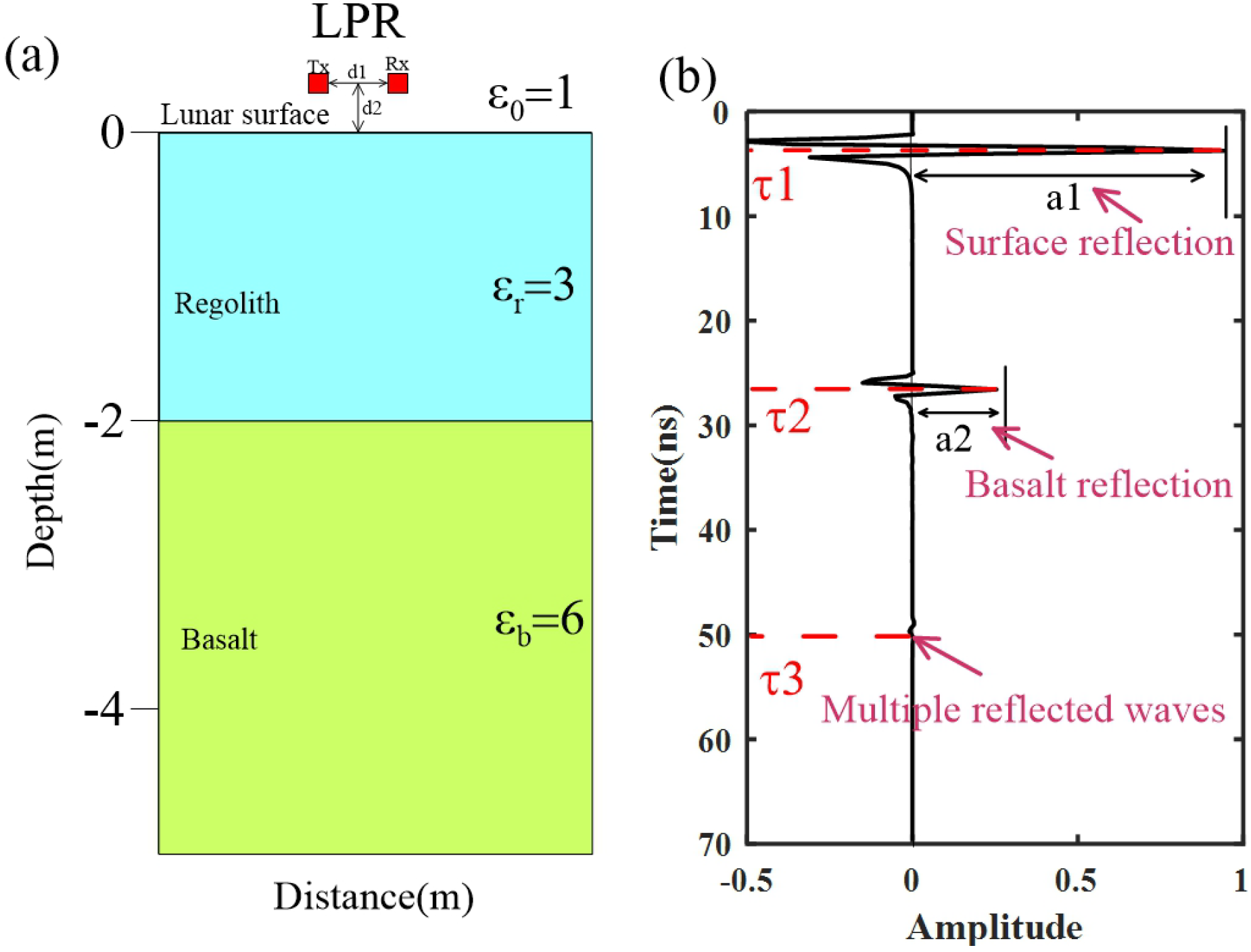
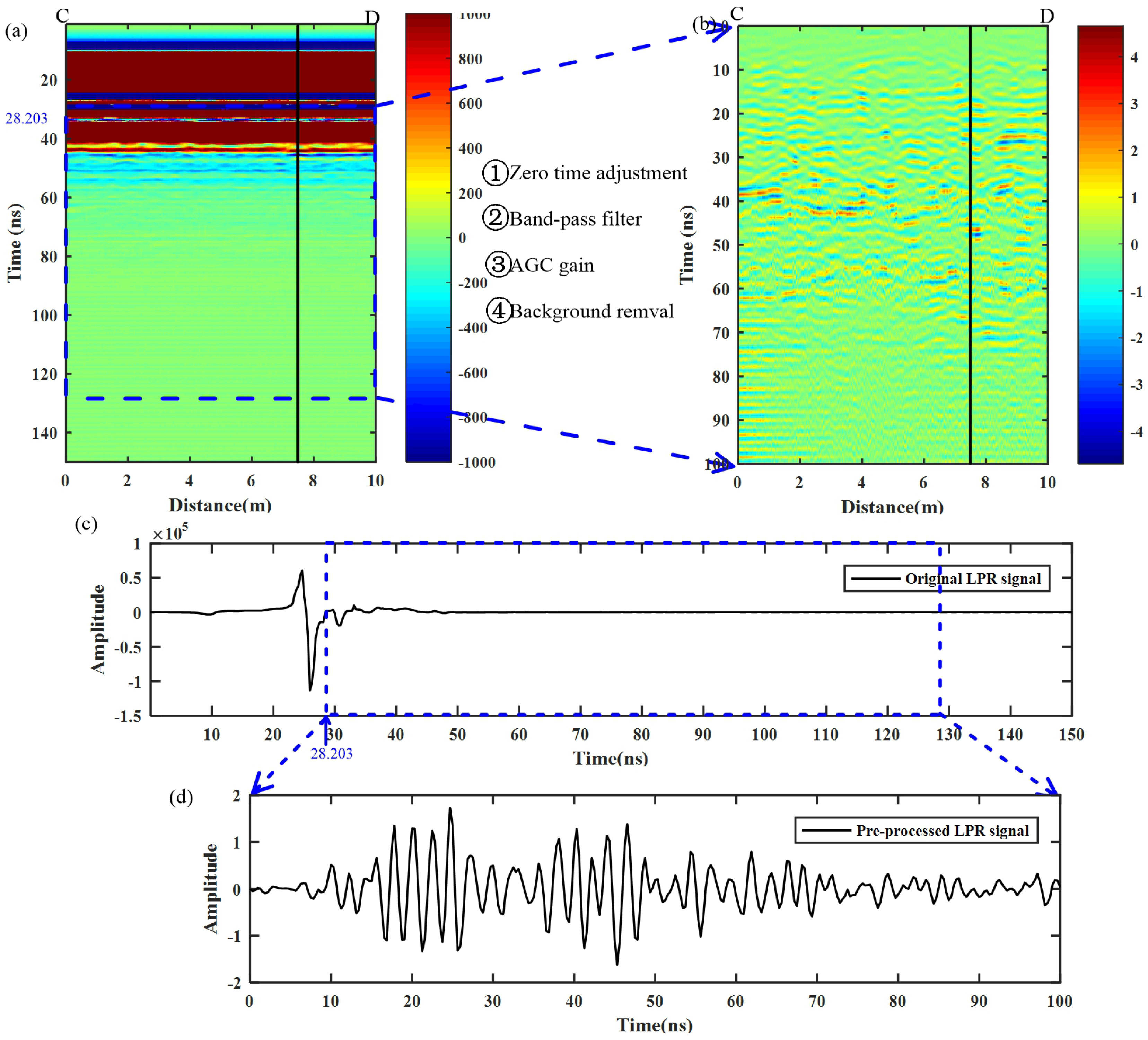
In this subsection, we present the performance analysis of the estimated parameters of the LPR data using the CS algorithm. In order to get $x\left(t\right)$, one calculates the LPR response of a 1D simple lunar regolith model (Figure 1a) using the finite-difference time-domain (FDTD) algorithm [29]. The simulation parameter settings are consistent with CE-3 Channel 2 [30] (

Table 1. Simulation parameters.

Parameter	Value	Direction
Height of antenna	0.3 m	d2 in Figure 1a
Offset of Tx and Rx	0.32 m	d1 in Figure 1a
Transmitted Waveform	Ricker	$g\left(t\right)$
Center frequency	500 MHz
Absorbing boundary	C-PML
Thickness of absorbing boundary	0.1 m	10 PML layers
Discrete grid	0.01 × 0.01 m	the size of the grid cells
Time step	0.03125 ns
Time window	70 ns

). The time step of the LPR is 0.3125 ns. Therefore, we need to sparse the simulation LPR data from 0.03125–0.3125 ns. The simulated amplitudes (${\left\{a_j\right\}}_{j=1}^L$) and time delays (${\left\{{\tau }_j\right\}}_{j=1}^L$) are listed in

Table 2. Amplitudes and time delays of $x\left(t\right)$.

Amplitude (a)	Value	Time Delay ($\mathit{\tau }$)	Value (ns)
a1	0.9421	$\tau$1	3.7500
a2	0.2546	$\tau$2	26.5625
a3	−0.0092	$\tau$3	49.6875

.

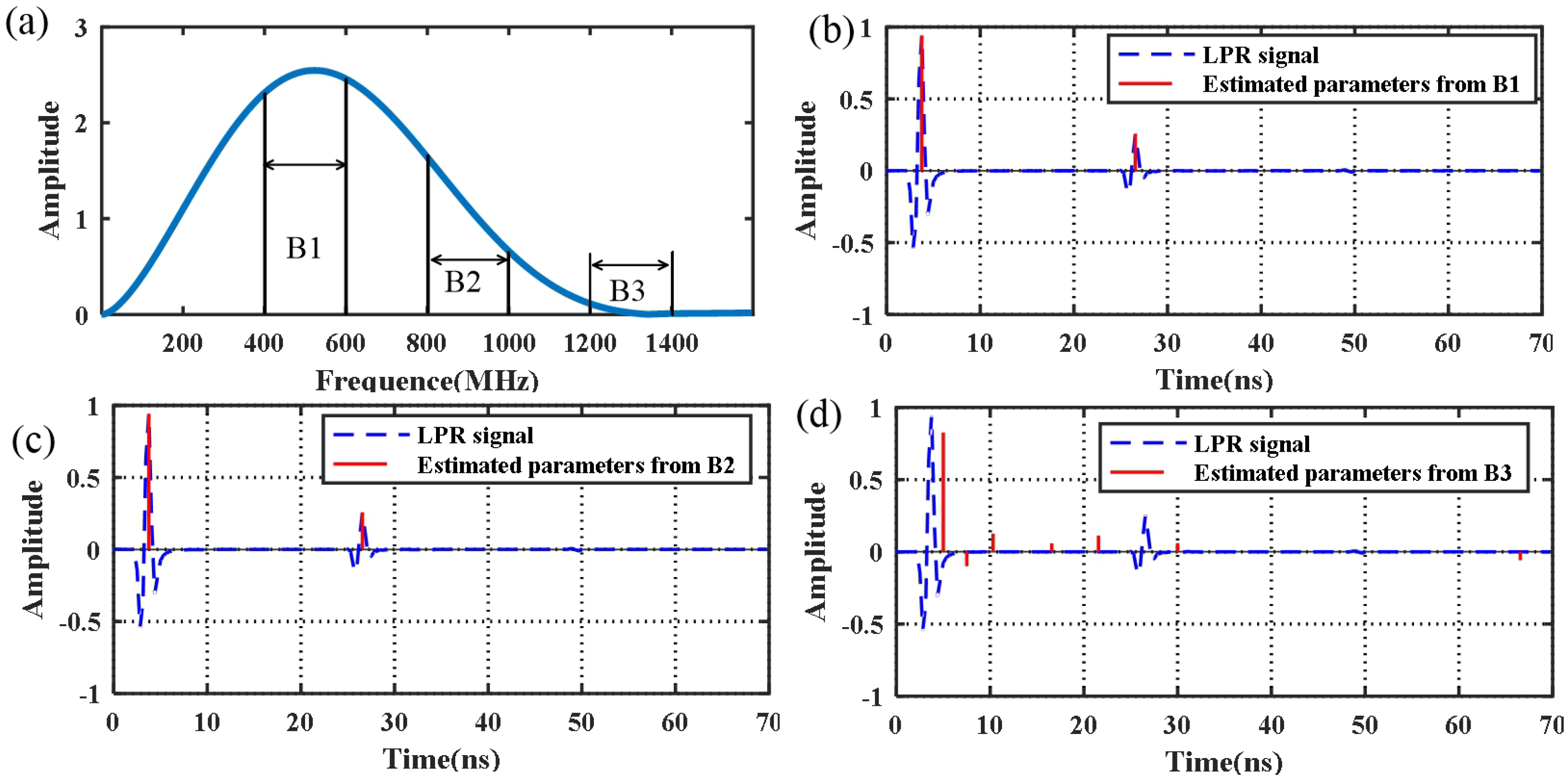
Figure 2a is the continuous time Fourier transformation ($G\left(\omega \right)$) of a 500-MHz Ricker. Obviously, LPR is a kind of ultra-wideband radar (UWB) [4] and has a large bandwidth (>1 GHz). In [19], Xia et al. stated that one can reconstruct radar signals in a larger subset of entries $\kappa$. In this study, we limited the bandwidth to improve the operational efficiency and increase the signal resolution from the noise.

For the first numerical experiment, we chose three subsets (Bandwidth 1 (B1), B2, B3; Figure 2a) of $\kappa$ and randomly selected 30 random Fourier series. The B1 bandwidth is from 400–600 MHz with $G\left(\frac{2\pi }{\tau }k\right)\ne 0$; the B2 bandwidth is from 800–1000 MHz with $G\left(\frac{2\pi }{\tau }k\right)\ne 0$; and the B3 bandwidth is from 1200–1400 MHz with $G\left(\frac{2\pi }{\tau }k\right)=0$.

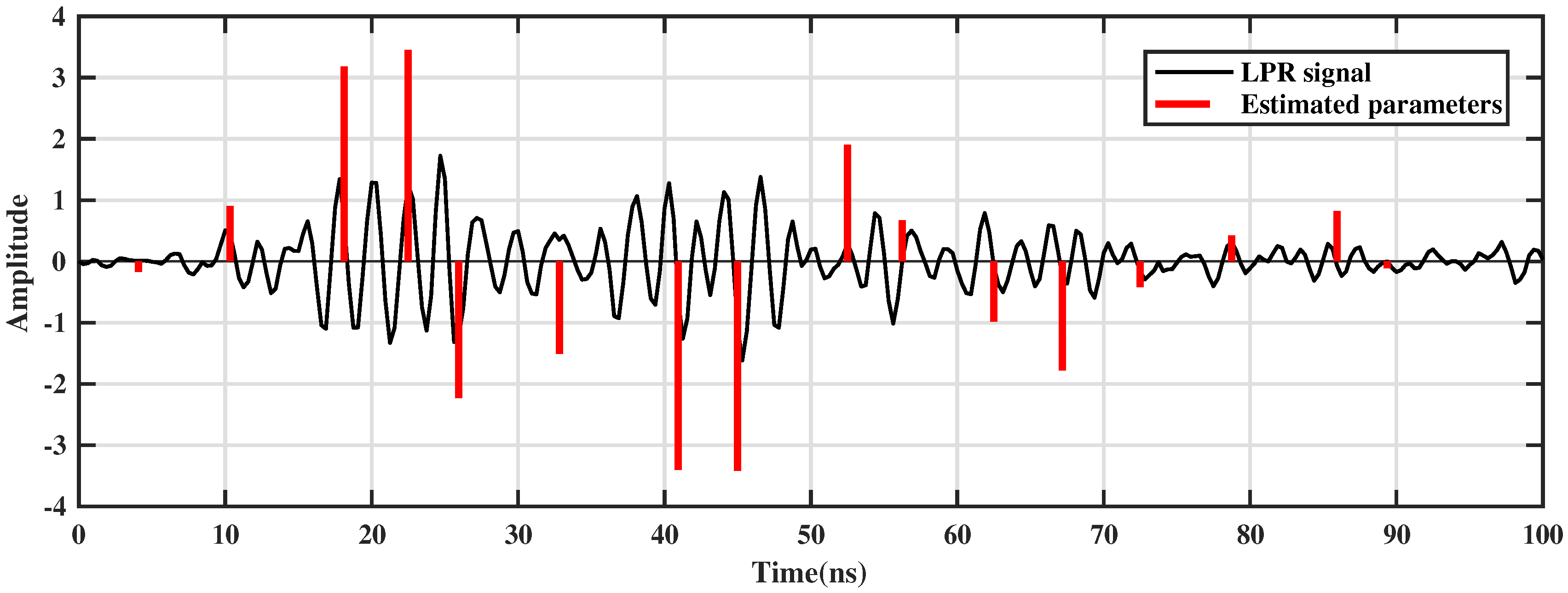
As this CS algorithm involves the random choice of parameters (Fourier coefficients), even if we set the same frequency band and number of Fourier coefficients, the estimated amplitudes and time delays will be different in each calculation (Figure 3). Therefore, in order to evaluate the performance of the CS algorithm accurately, for the final value in the numerical experiment, we used the average value obtained by executing the algorithm 60 times, selected by checking the convergence of its results. The standard deviation information is given to describe the stability of the algorithm. In Figure 3, the average value (AVG) is 0.2553 and the standard deviation ($\sigma$) is 0.0025. Obviously, this CS algorithm is stable. To account for the possibility of processing data collected over a larger spatial scale, we recorded the time cost of the numerical experiments. The parameters of the computer used to execute the numerical experiment are listed in

Table 3. The parameters of the computer used to execute the numerical experiment.

Type	Laptop
Operating system	Microsoft Windows 10
CPU	Intel(R) Core(TM) i7-6820HQ
RAM	16 GB

.

Figure 2 shows the results of parameter estimation in different bandwidth subsets. The estimated amplitudes ${\left\{a_j\right\}}_{j=1}^L$ and time delays ${\left\{{\tau }_j\right\}}_{j=1}^L$ are listed in

Table 4. Estimated parameter value statistics table of the first numerical experiment.

Frequency Band (MHz)	Amplitudes (a), Time Delays ($\mathit{\tau }$)	Value	err_rel (%)	Standard Deviation ($\mathit{\sigma }$)	Time Cost (s)
B1[400–600]	a1	0.9421	0	0.0006	160
	a2	0.2553	0.3	0.0025
	a3	0	∼	∼
	$\tau$1	3.7500 ns	0	0
	$\tau$2	26.5625 ns	0	0
	$\tau$3	∼	∼	∼
B2[800–1000]	a1	0.9420	0.1	0.004	159
	a2	0.2570	1.0	0.0045
	a3	0	∼	∼
	$\tau$1	3.7500 ns	0	0
	$\tau$2	26.5625 ns	0	0
	$\tau$3	∼	∼	∼
B3[1200–1400]	a1	0.8325	11.63	0.2	160
	a2	0	∼	∼
	a3	0	∼	∼
	$\tau$1	6.0 ns	60	3
	$\tau$2	∼	∼	∼
	$\tau$3	∼	∼	∼

. The relative error between the estimated value and the simulated value (Table 2) is defined as err_rel (%).

According to the results, both B1 and B2 can estimate amplitudes and time delays very well, and the amplitudes calculated by B1 have more accurate results. However, in B3, as mentioned in the theorysection, since the smaller value of the Fourier series coefficients and a part of $G\left(\frac{2\pi }{\tau }k\right)$ approximate to zero, the CS algorithm cannot accurately estimate the parameters. Considering that the center frequency of $g\left(t\right)$ (500 MHz) is included in B1 ([400–600] MHz), we recognize that the CS algorithm can obtain an accurate estimation of the signal parameters from the LPR data using a random Fourier series subset within a limited bandwidth around the center frequency. To gain a better understanding of the performance and reliability of the algorithm and to identify the best settings (the number of Fourier series coefficients and the bandwidth extension), we conducted a second and third numerical experiment with a focus on controlling the variables.

In the second numerical experiment, the number of Fourier series was fixed to 30, and the frequency bandwidths were set at 30% (B4[425–575] MHz), 50% (B5[375–625] MHz), and 60% (B6[350–650] MHz) of the central frequency, with centering on the central frequency (500 MHz). The results are listed in

Table 5. Estimated parameter value statistics table of the second numerical experiment.

Frequency Band (MHz)	Amplitudes (a), Time Delays ($\mathit{\tau }$)	Value	err_rel (%)	Standard Deviation ($\mathit{\sigma }$)	Time Cost (s)
B4[425–575]	a1	0.9421	0	0.0002	113
	a2	0.2550	0.3	0.0015
	a3	0	∼	∼
	$\tau$1	3.7500 ns	0	0
	$\tau$2	26.5625 ns	0	0
	$\tau$3	∼	∼	∼
B5[375–625]	a1	0.9420	0.1	0.004	265
	a2	0.2565	0.9	0.0036
	a3	0	∼	∼
	$\tau$1	3.7500 ns	0	0
	$\tau$2	26.5625 ns	0	0
	$\tau$3	∼	∼	∼
B6[350–650]	a1	0.9420	0.1	0.005	402
	a2	0.2568	0.9	0.0062
	a3	0	∼	∼
	$\tau$1	3.7500 ns	0	0
	$\tau$2	26.5625 ns	0	0
	$\tau$3	∼	∼	∼

. From those results, the accuracy and reliability of the CS algorithm are satisfactory for the three frequency bands. When the frequency range is extended from B1–B5 MHz, there is a rather significant change of the algorithm performance: the error becomes higher and similar to the error obtained in B2. In order to achieve a better estimated accuracy over a larger bandwidth, the number of Fourier coefficients needs to be increased. In other words, the number of Fourier series needs to meet a certain density in the frequency band. However, the increase of Fourier series density reduces the randomness of the algorithm. In our CS algorithm, a random Fourier series can increase the resolution of the underlying signal in actual LPR data. We also noticed that, although a larger bandwidth can provide increased randomness in Fourier series selection, time costs and estimation errors increase: when the bandwidth increases from 150 to 300 MHz, the time cost increases by 2.5 times.

In the third numerical experiment, the frequency range was fixed to B1[400–600] MHz, and the number of Fourier series was set at 10 or 60. The results are listed in

Table 6. Estimated parameter value statistics table of the third numerical experiment.

Number of Fourier Series	Amplitudes (a), Time Delays ($\mathit{\tau }$)	Value	err_rel (%)	Standard Deviation ($\mathit{\sigma }$)	Time Cost (s)
10	a1	0.9323	1	0.1049	152
	a2	0.2050	20.1	0.0473
	a3	0	∼	∼
	$\tau$1	3.7500 ns	0	0.01
	$\tau$2	26.5625 ns	0	0.01
	$\tau$3	∼	∼	∼
60	a1	0.9421	0	0.0001	192
	a2	0.2550	0.1	0.0002
	a3	0	∼	∼
	$\tau$1	3.7500 ns	0	0
	$\tau$2	26.5625 ns	0	0
	$\tau$3	∼	∼	∼

. In this numerical experiment, we cannot accurately estimate the amplitude and time delay using a random Fourier series subset with 10 coefficients. The CS algorithm requires a sufficient number of Fourier series coefficients to ensure reliability. By doubling the number of Fourier coefficients (from 30 to 60), a higher stability of the algorithm can be achieved (in terms of smaller standard deviation) at a limited additional computational cost (only 20% longer execution time). Although we decided to work with 30 coefficients in this paper, in some future scenarios, it may be useful to use more coefficients. However, an increase in the number of Fourier series, such as the 60 Fourier series in Table 6, means an increase in time cost and a decrease in randomness.

Therefore, considering the estimation error, randomness, and time cost, a random Fourier series subset with 30 coefficients chosen within 400–600 MHz is one of the best settings for 500-MHz LPR data processing. The CS algorithm can be executed on a personal computer. Single trace data can be processed in a few minutes. However, if, in some cases, we need to increase the frequency range and the number of Fourier series, the increase in time cost is inevitable. In addition, the time cost limitations of this CS algorithm are also possible when dealing with larger scale problems.

In order to assess the anti-interference ability and robustness of the CS algorithm, we designed the fourth and fifth numerical experiments with noise.

In the fourth numerical experiment, we added two sine interferences to $x\left(t\right)$ using Equation (12) (Figure 4).

$$x\left(t\right)=x\left(t\right)+sin(2\pi \ast M_1\ast t)\ast 0.1+sin(2\pi \ast M_2\ast t)\ast 0.2$$

(12)

where ($M_1$, $M_2$) is the frequency of the sine interference and was set at (200 MHz, 800 MHz) and (450 MHz, 550 MHz). The parameter values were estimated by the CS algorithm using 30 random Fourier series in B1(400–600 MHz). The results are listed in

Table 7. Estimated parameter value statistics table of the fourth numerical experiment.

Frequency of Sine Wave (MHz)	Amplitudes (a), Time Delays ($\mathit{\tau }$)	Value	err_rel (%)	Standard Deviation ($\mathit{\sigma }$)	Time Cost (s)
200,800	a1	0.9749	3	0.001	162
	a2	0.2414	5	0.001
	a3	0	∼	∼
	$\tau$1	3.7500 ns	0	0
	$\tau$2	26.5625 ns	0	0
	$\tau$3	∼	∼	∼
450,550	a1	0.98531	5	0.05	169
	a2	0.2358	7	0.03
	a3	0	∼	∼
	$\tau$1	3.7500 ns	0	0
	$\tau$2	26.5625 ns	0	0
	$\tau$3	∼	∼	∼

. The accuracy of the CS algorithm is satisfactory. Since the Fourier series in our CS algorithm is discontinuous and random, although 450 and 550 MHz are included in the frequency range (400∼600 MHz), we can still accurately estimate the amplitude and time delays.

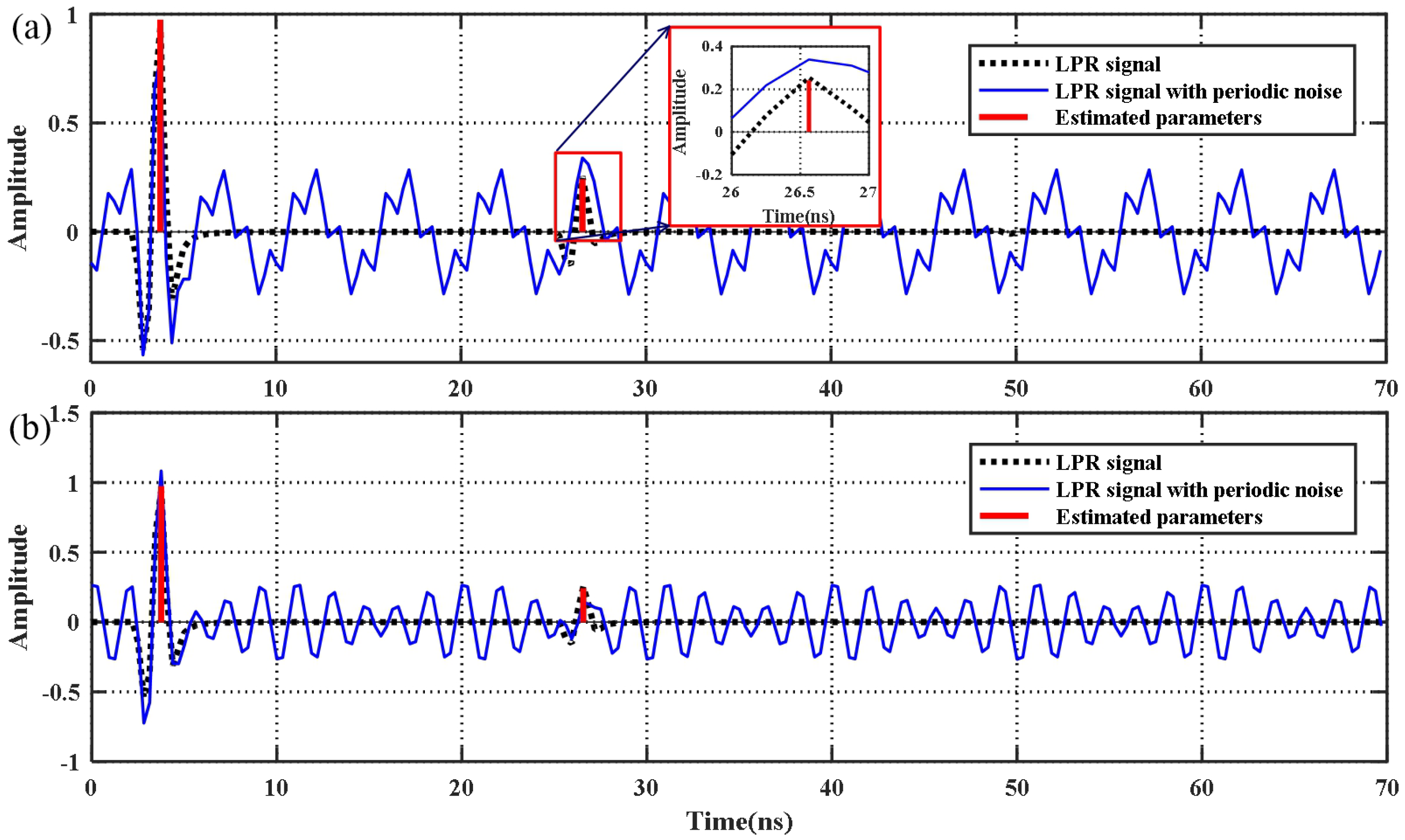
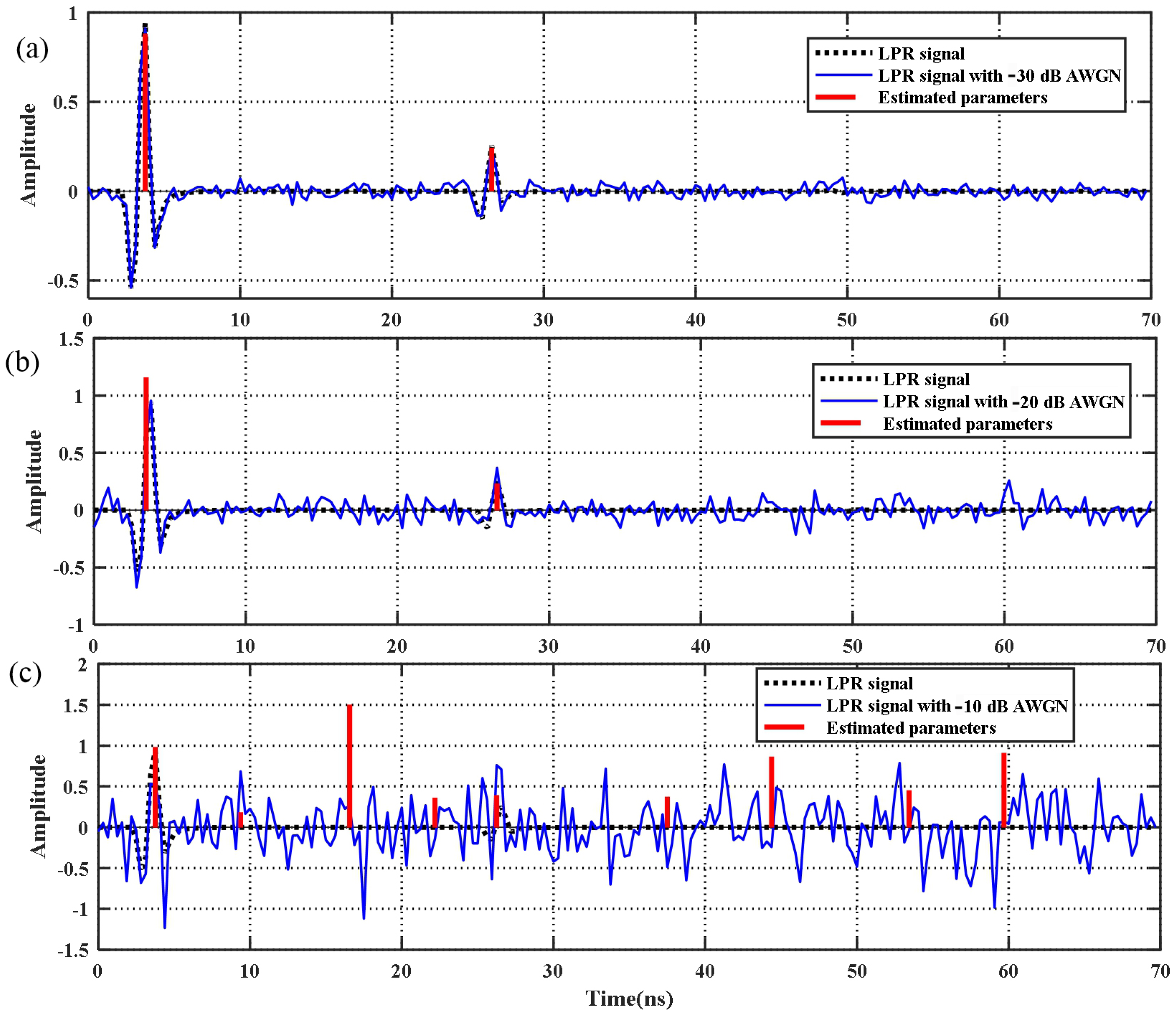
In the fifth numerical experiment, we added −30, −20, and −10 dB of additive white Gaussian noise (AWGN) to $x\left(t\right)$ (Figure 5). The noise level is defined by the following formula:

$$AWGN\_dB=10{log}_{10}\frac{P\_n}{P\_s},$$

(13)

where $P\_n$ is the noise signal power and $P\_s$ is the original signal power.

The parameter values were determined by the CS algorithm using 30 random Fourier series in B1(400–600 MHz). The results are listed in

Table 8. Estimated parameter value statistics table of the fifth numerical experiment.

AWGN Noise Level (dB)	Amplitudes (a), Time Delays ($\mathit{\tau }$)	Value	err_rel (%)	Standard Deviation ($\mathit{\sigma }$)	Time Cost (s)
30	a1	0.8802	7	0.002	169
	a2	0.2450	0.3	0.003
	a3	0	∼	∼
	$\tau$1	3.7500 ns	0	0
	$\tau$2	26.5625 ns	0	0
	$\tau$3	∼	∼	∼
20	a1	1.125	20	0.05	170
	a2	0.2315	9	0.06
	a3	0	∼	∼
	$\tau$1	3.2500 ns	12	0
	$\tau$2	26.5625 ns	0	0
	$\tau$3	∼	∼	∼
10	a1	1.022	0.8	0.2	165
	a2	∼	∼	∼
	a3	∼	∼	∼
	$\tau$1	3.7500 ns	0	∼
	$\tau$2	∼	∼	∼
	$\tau$3	∼	∼	∼

.

Obviously, the signal parameters can be accurately estimated from signals with noise in general (Figure 5a,b). Due to the wide frequency range of the AWGN, when the noise level is 10 dB (Figure 5c), the CS algorithm cannot distinguish between the reflection signal and the false waveform generated by the AWGN. This requires researchers to apply their judgment in practical applications.

These numerical experiments indicate that the CS algorithm used with a random Fourier series can estimate a target’s signal parameters from noisy LPR data. This CS algorithm can reconstruct the amplitudes and time delays with high efficiency and high precision under an appropriate bandwidth and Fourier series.

3. Algorithm Verification Using 2D the Random Regolith Model

In order to verify that the CS algorithm is effective for LPR data, we built a complex lunar regolith model (Figure 6) and calculated the LPR response using the 2D FDTD algorithm [29]. We set the numerical simulation parameters to be the same as those in the numerical experiment described in Section 2.3; the parameters are presented in Table 1 in Section 2. The LPR moving route was from 1–9 m in distance, and the sampling interval on the moving route was 0.05 m.

The model size was 10 m in the horizontal direction and 6 m in the vertical direction. To make the model structure similar to real lunar regolith, the following settings were applied.

(1)

The relative permittivity is proportional to the depth. The average relative permittivity of the lunar regolith is 3.0. Therefore, we improved the formula of the relationship between relative permittivity and depth [31,32] as follows:

$${\epsilon }_r={1.919}^{1.92\frac{z+12.2}{z+18}}+0.4$$

(14)

(2)

A Gaussian random field was used to model the regolith. A great deal of natural science data display marked Gaussian characteristics [33,34,35]. We built the lunar regolith relative permittivity model with clipped Gaussian random field theory [36]. A relative permittivity that is set from 2.5–3.5 satisfies the Gaussian random distribution.

(3)

The formation of lunar regolith indicates the existence of detritus [6]. In the LPR data, most reflections are formed by basalt debris [7]. Three strongly-reflecting debris materials (A: a square with a side length of 0.1 m; B: a circle with a radius of 0.1 m; C: a square with a side length of 0.2 m; Figure 6a) were incorporated into the 2D regolith model with the same relative permittivity as basalt (${\epsilon }_b=6$).

Figure 7a is a snapshot of a radar wave in 28.8 ns at 5 m. The distortion of electromagnetic waves passing through random inhomogeneous media is clearly visible. Figure 7b shows the forward simulation result with direct waves removed. In the simulated LPR data image, the response of the strongly-reflecting debris is mixed with the response of weak reflectors in a random medium. The parameter values were estimated by the CS algorithm using 30 random Fourier series in B1 (400–600 MHz). Figure 8a is a single trace at 5 m (red line in Figure 7b) and the amplitudes and the time delays estimated by the CS algorithm. The CS algorithm not only accurately estimates the time delays (${\left\{{\tau }_j\right\}}_{j=1}^L$) of a strong reflection response, but also restores the amplitudes (${\left\{a_j\right\}}_{j=1}^L$). Figure 8b is the color image of absolute amplitudes ($\mid {\left\{a_j\right\}}_{j=1}^L\mid$). Compared to the original LPR image (Figure 7b), responsive recognition is greatly improved. According to the amplitude’s absolute value, the reflected response signal can be located and identified. Moreover, some LPR responses of small debris in random inhomogeneous media are available. One can identify some complete weak responses based on the continuity of the amplitude to enrich the interpretation process.

4. Processing and Analyzing LPR Data

4.1. Preprocessing

LPR is one of the important scientific systems onboard the Yutu lunar rover in the scope of China’s Chang’E-3 lunar mission. The CE-3 landing site is in northern Mare Imbrium at 44.1213°N, 19.5115°W at an elevation of −2.627 km [6]. The Yutu lunar rover’s route is shown in Figure 9. The raw LPR data are archived and distributed by the National Astronomical Observatories, Chinese Academy of Sciences (NAOC) (http://moon.bao.ac.cn/) [13]. In this paper, we focus on the data collected by the 500-MHz Level 2C data (a band-pass filter based on fast Fourier transform (FFT) filtering was done [7,13]) from C to D (Figure 9). The distance of the CD route is 10 m.Considering the unique characteristics of LPR data acquisition, we performed a longitudinal displacement correction, removing the repeating paths and velocity interpolation to extract the LPR data (Figure 10a) from the raw data [7]. Although the LPR data were successfully extracted, it is difficult to strip the direct waves from the original data. According to calibration tests that were performed by the Institute of Electronics, Chinese Academy of Sciences, the time delay of the radar echo signal transmitted from the lunar surface is 28.203 ns for Channel 2; thus, the lunar surface is characterized by a 28.203-ns time delay correction [30]. Then, we applied an automatic gain control (AGC) method to recover the amplitude loss from spreading and scattering [2] and removed the background using a median filter, as is usually used for GPR data for Earth-based applications. Since most of the effective information of the 500-MHz LPR data are concentrated within 100 ns [6,7], we only processed the data between 0 and 100 ns.

4.2. Parameter Estimation Using the CS Algorithm

Based on the numerical experiments’ results in the theoretical part of this study, we randomly selected 30 Fourier series coefficients from 200–600 MHz to estimate the amplitudes and time delays using the CS algorithm. Figure 11 is a single trace of the LPR data and the parameters estimated by the CS-based approach. From Figure 11, we can see that the estimated parameters are quite consistent with the preprocessed LPR data (Figure 11b). The aliased waveform image was converted to clear discrete reflection amplitudes and time delays. Figure 12 shows the CD LPR profile data overlaid with the processing results. In Figure 12, due to the time delay correction and the removal of the background, the surface reflection signal is missing. Time delays were distributed between 10 and 70 ns. Below 70 ns, although the sporadic reflected signals could be identified, the amplitude was smaller and discontinuous. In order to highlight the response of a reflector in the regolith, we provide a color image of the absolute amplitude (Figure 13) with a threshold ($\mid {\left\{a_j\right\}}_{j=1}^L\mid >1.5$). Compared with the continuous waveforms in raw data, the CS algorithm more easily locates and extracts reflections caused by buried targets. By analyzing the continuity of the time delays and the values of the amplitudes, we can reconstruct and identify response signals caused by discrete reflectors beneath the lunar surface (Figure 14).

4.3. Results

When combining the forming mechanism of the regolith in the study area with the result of the CS-based approach, a further interpretation of the LPR data was revealed (Figure 14). A dielectric permittivity of 3.0 + i0.03 was used to calculate the depth. In the LPR data image, a three-layer structure could be clearly delimited as follows.

• The top layer (depth < 1 m) cannot extract reflection parameters at all. This is the fine-grained regolith part of the lunar regolith. In [6], this part was interpreted as a reworked zone. Even though the fine-grained regolith was composed of numerous layers, the layer thickness was typically on the order of several centimeters [37], which is much smaller than the LPR range resolution [4]. Therefore, it is difficult to extract the reflected signal from this layer.
• The middle layer (buried from 1–7 m) had the most signal reflectors beneath the lunar surface. It is the paleoregolith of mare basalt with much debris. After the processing step in the CS-based approach, the reflective response signal, which is difficult to extract from the original LPR data, became clear (Figure 13). The size of the reflection curve is often proportional to the volume of the debris [7]. On the basis of the continuity and the absolute value of the estimated amplitude, some reflection response signals are marked by a red curve in Figure 14. Obviously, this is a good improvement for evaluating the LPR data.
• The last part is the basalt base. Since there is no obvious reflective interface between the regolith and mare basalt, one can distinguish this region by the distribution of a strong reflection response signal. Obviously, from Figure 13, there were no reflection signals ($\mid {\left\{a_j\right\}}_{j=1}^L\mid >1.5$). The estimated reflection response at [I] (Figure 13) is a false reflection, considering the unusually persistent periodicity of this part of the LPR data.

4.4. Discussion

In the 2D random regolith model, a strong interface between the regolith and basalt is present. However, in the measured 500-MHz LPR data, there is no obvious reflective interface between the regolith and mare basalt. It is possible that there is a smooth variation in the permittivity on the interface. The overall reflection generated by a gradual interface has a different shape than the transmitted pulse [38], whereas a sudden permittivity change generates a reflection having a different amplitude, but the same shape as the transmitted pulse. This is a challenge for the CS algorithm. We hope to study this scenario in future work.

When the CS-based approach is applied to LPR data, there is an improvement in classifying the stratigraphic structure of the lunar regolith. The stratification result is consistent with previous studies [6,7,16], and we located the debris in the regolith. Moreover, the improvement in LPR data interpretation is not limited to this. It can provide a relatively accurate initial model for standard focusing methods (migration, beamforming, diffraction tomography, etc.). Accurate amplitudes and time delays also can significantly refine the accuracy of estimated lunar regolith parameters, such as permittivity and iron–titanium content [2,16]. It is critical to quantify potential resources for lunar exploration and for the engineering of human outposts.

5. Conclusions

In this paper, we propose a compressive sensing-based approach to reconstruct the amplitudes and the time delays of radar data. Numerical analysis of the CS-based approach performance was conducted and is herein discussed. The simulation results show that the approach is effective and stable. Then, successful estimations of the amplitudes and the time delays of the 500-MHz LPR data using the compressive sensing-based approach were achieved. The final result shows that the CS-based approach can improve the capability of extracting a target’s response signal from a complex lunar environment. In addition, these results provide valuable information about the lunar regolith structure and estimated parameters, such as the electrical parameters and the iron–titaniumcontent of the regolith.

References

1. Russell, P.S.; Grant, J.A.; Williams, K.K.; Carter, L.M.; Garry, W.B.; Daubar, I.J. Ground penetrating radar geologic field studies of the ejecta of barringer meteorite crater, arizona, as a planetary analog. J. Geophys. Res. Planets 2013, 118, 1915–1933. [Google Scholar] [CrossRef]
2. Lai, J.; Xu, Y.; Zhang, X.; Tang, Z. Structural analysis of lunar subsurface with Chang’E-3 lunar penetrating radar. Planet. Space Sci. 2016, 120, 96–120. [Google Scholar] [CrossRef]
3. One, T.; Kumamoto, A.; Kasahara, K.; Yamaguchi, Y.; Yamaji, A.; Kobayashi, T.; Oshigami, S.; Nakagawa, H.; Goto, Y.; Hashimoto, K.; et al. The Lunar Radar Sounder (LRS) Onboard the KAGUYA (SELENE) Spacecraft. Space Sci. Rev. 2010, 154, 145–192. [Google Scholar] [CrossRef]
4. Fang, G.; Zhou, B.; Ji, Y.; Zhang, Q.; Shen, S.; Li, Y. Lunar penetrating radar onboard the Chang’E-3 mission. Res. Astrono. Astrophys. 2014, 14, 1607–1622. [Google Scholar] [CrossRef]
5. Porcello, L.J.; Jordan, R.L.; Zelenka, J.S. The Apollo lunar sounder radar system. Proc. IEEE 1974, 62, 769–788. [Google Scholar] [CrossRef]
6. Fa, W.; Zhu, M.; Liu, T.; Plescia, J.B. Regolith stratigraphy at the chang’e-3 landing site as seen by lunar penetrating radar. Geophys. Res. Lett. 2016, 42, 10179–10187. [Google Scholar] [CrossRef]
7. Zhang, L.; Zeng, Z.; Li, J.; Lin, J.; Hu, Y.; Wang, X. Simulation of the lunar regolith and lunar-penetrating radar data processing. IEEE J. Sel. Top. Appl. Earth Obs. Remote. Sens. 2018, 11, 655–663. [Google Scholar] [CrossRef]
8. Zhang, J.; Yang, W.; Hu, S.; Lin, Y.; Fang, G.; Li, C. Volcanic history of the imbrium basin: A close-up view from the lunar rover Yutu. Proc. Natl. Acad. Sci. USA 2015, 112, 5342–5347. [Google Scholar] [CrossRef] [PubMed]
9. Papike, J.J.; Simon, S.B.; Laul, J.C. The lunar regolith: Chemistry, mineralogy, and petrology. Rev. Geophys. 1982, 20, 761–826. [Google Scholar] [CrossRef]
10. Fa, W.; Wieczorek, M.A. Regolith thickness over the lunar nearside: Results from earth-based 70-cm arecibo radar Obs. Icarus 2012, 218, 771–787. [Google Scholar] [CrossRef]
11. Papike, J.J.; Simon, S.B.; Laul, J.C. The lunar regolith: Chemistry, mineralogy, and petrology. Rev. Geophys. 1982, 20, 761–826. [Google Scholar] [CrossRef]
12. Wilcox, B.B.; Robinson, M.S.; Thomas, P.C.; Hawke, B.R. Constraints on the depth and variability of the lunar regolith. Meteorit. Planet. Sci. 2015, 40, 695–710. [Google Scholar] [CrossRef]
13. Sun, Y.; Fang, G.Y.; Feng, J.; Xing, S.; Jing, Y.; Zhou, B. Data processing and initial results of Chang’E-3 lunar penetrating radar. Res. Astron. Astrophys. 2014, 14, 1623–1632. [Google Scholar]
14. Dong, Z.; Fang, G.; Ji, Y.; Gao, Y.; Wu, C.; Zhang, X. Parameters and structure of lunar regolith in chang’e-3 landing area from lunar penetrating radar (lpr) data. Icarus 2016, 282, 40–46. [Google Scholar] [CrossRef]
15. Feng, J.; Su, Y.; Ding, C.; Xing, S.; Dai, S.; Zou, Y. Dielectric properties estimation of the lunar regolith at CE-3 landing site using lunar penetrating radar data. Icarus 2017, 284, 424–430. [Google Scholar] [CrossRef]
16. Zhang, L.; Zeng, Z.; Li, L.; Huang, L.; Huo, Z.; Wang, K.; Zhang, J. Parameter Estimation of Lunar Regolith from Lunar Penetrating Radar Data. Sensors 2018, 18, 2907. [Google Scholar] [CrossRef] [PubMed]
17. Delbo, S.; Gamba, P.; Roccato, D. A fuzzy shell clustering approach to recognize hyperbolic signatures in subsurface radar images. IEEE Trans. Geosci. Remote. Sens. 2002, 38, 1447–1451. [Google Scholar] [CrossRef]
18. Ambrosanio, M.; Pascazio, V. A compressive-sensing-based approach for the detection and characterization of buried objects. IEEE J. Sel. Top. Appl. Earth Obs. Remote. Sens. 2017, 8, 3386–3395. [Google Scholar] [CrossRef]
19. Xia, S.; Liu, Y.; Sichina, J.; Liu, F. A compressive sensing signal detection for uwb radar. Prog. Electromagn. Res. 2013, 141, 479–495. [Google Scholar] [CrossRef]
20. Gurbuz, A.C.; McClellan, J.H.; Scott, W.R., Jr. Compressive sensing for subsurface imaging using ground penetrating radar. Signal Process. 2009, 89, 1959–1972. [Google Scholar] [CrossRef]
21. Zhu, L.; Zhu, Y.; Mao, H.; Gu, M. A New Method for Sparse Signal Denoising Based on Compressed Sensing. Second. Int. Symp. Knowl. Acquis. Model. 2009, 1, 35–38. [Google Scholar]
22. Metzler, C.A.; Maleki, A.; Baraniuk, R.G. From denoising to compressed sensing. IEEE Trans. Inf. Theory 2016, 62, 5117–5144. [Google Scholar] [CrossRef]
23. Maravic, I.; Vetterli, M. Sampling and reconstruction of signals with finite rate of innovation in the presence of noise. IEEE Trans. Signal Process. 2005, 53, 2788–2805. [Google Scholar] [CrossRef] [Green Version]
24. Vetterli, M.; Marziliano, P.; Blu, T. Sampling signals with finite rate of innovation. IEEE Trans. Signal Process. 2002, 50, 1417–1428. [Google Scholar] [CrossRef] [Green Version]
25. Michaeli, T.; Eldar, Y.C. Xampling at the rate of innovation. IEEE Trans. Signal Process. 2012, 60, 1121–1133. [Google Scholar] [CrossRef]
26. Candès, E.; Fernandez-Granda, C. Towards a mathematical theory of superresolution. Commun. Pure Appl. Math. 2013, 67, 906–956. [Google Scholar] [CrossRef]
27. Gedalyahu, K.; Tur, R.; Eldar, Y. Multichannel sampling of pulse streams at the rate of innovation. IEEE Trans. Signal Process. 2011, 59, 1491–1504. [Google Scholar] [CrossRef]
28. Tang, G.; Bhaskar, B.N.; Shah, P.; Recht, B. Compressed sensing off the grid. IEEE Trans. Inf. Theory 2013, 59, 7465–7490. [Google Scholar] [CrossRef]
29. Irving, J.; Knight, R. Numerical modeling of ground-penetrating radar in 2-d using matlab. Comput. Geosci. 2006, 32, 1247–1258. [Google Scholar] [CrossRef]
30. Zhou, N.; Zhou, P.; Yang, K.; Yuan, Y.; Gou, S. The preliminary processing and analysis of LPR channel-2b data from chang’e-3. Sci. China Phys. Mech. Astron. 2014, 57, 2346–2353. [Google Scholar] [CrossRef]
31. Dollfus, A. Physical properties of the lunar surface. Catal. Ind. 2014, 6, 114–121. [Google Scholar]
32. Kobayashi, T.; Kim, J.H.; Lee, S.R.; Araki, H.; Ono, T. Simultaneous observation of lunar radar sounder and laser altimeter of kaguya for lunar regolith layer thickness estimate. IEEE GeoSci. Remote. Sens. Lett. 2010, 7, 435–439. [Google Scholar] [CrossRef]
33. Haran, M. Gaussian random field models for spatial data. Handb. Markov Chain. Mt-Carlo 2009, 449–478. [Google Scholar]
34. Jiang, Z.; Zeng, Z.; Li, J.; Liu, F.; Li, W. Simulation and analysis of GPR signal based on stochastic media model with an ellipsoidal autocorrelation function. J. Appl. Geophys. 2013, 99, 91–97. [Google Scholar] [CrossRef]
35. Zeng, Z.; Chen, X.; Li, J.; Chen, L.; Lu, Q.; Liu, F. Recursive impedance inversion of ground-penetrating radar data in stochastic media. Appl. Geophys. 2015, 12, 615–625. [Google Scholar] [CrossRef]
36. Li, J.; Zeng, Z.; Liu, C.; Huai, N.; Wang, K. A study on lunar regolith quantitative random model and lunar penetrating radar parameter inversion. IEEE GeoSci. Remote. Sens. Lett. 2017, 14, 1953–1957. [Google Scholar] [CrossRef]
37. Mitchell, J.; Carrier, W.; Costes, N.C.; Houston, W.; Scott, R. Surface Soil Variability and Stratigraphy at the Apollo 16 Site. Geochim. Cosmochim. Acta 1973, 3, 2437–2445. [Google Scholar]
38. Prokopovich, I.; Popov, A.; Pajewski, L.; Marciniak, M. Application of Coupled-Wave Wentzel-Kramers- Brillouin Approximation to Ground Penetrating Radar. Remote. Sens. 2017, 10, 22. [Google Scholar] [CrossRef]
Figure 1. (a) The 1D lunar regolith model (Rx: receive antenna; Tx: transmitting antenna) and (b) the LPR response signal of the 1D lunar regolith model with the direct waves removed ( x ( t ) ).
Remotesensing 10 01925 g001
Figure 2. The results of the first numerical experiment. (a) The continuous time Fourier transformation of g ( t ) . (b) Estimated parameters by the CS algorithm in Bandwidth 1 (B1). (c) Estimated parameters by the CS algorithm in B2. (d) Estimated parameters by the CS algorithm in B3.
Remotesensing 10 01925 g002
Figure 3. Estimated value of a2 from B1 obtained by executing the CS algorithm 60 times for numerical experiments. The average value (AVG) is 0.2553, and the standard deviation ( σ ) is 0.0025.
Remotesensing 10 01925 g003
Figure 4. LPR data with periodic noise and parameters estimated by the CS algorithm. (a) The frequencies of the sine interference are 200 and 800 MHz; (b) the frequencies of the sine interference are 450 and 550 MHz).
Remotesensing 10 01925 g004
Figure 5. LPR data with Gaussian noise and the parameters estimated by the CS algorithm. (a) Noise level: −30 dB; (b) noise level: −20 dB; (c) noise level: −10 dB.
Remotesensing 10 01925 g005
Figure 6. (a) The 2D random regolith model. (b) Permittivity trend at 5 m (black dotted line in (a)).
Remotesensing 10 01925 g006
Figure 7. (a) A snapshot of a radar wave in 28.8 ns at 5 m. (b) Simulation results of the 2D regolith model.
Remotesensing 10 01925 g007
Figure 8. (a) A single trace in 5 m (red line in Figure 7b) and the parameters estimated by the CS algorithm. (b) Image of the estimated absolute amplitudes of the simulated LPR profile.
Remotesensing 10 01925 g008
Figure 9. Yutu lunar rover’s route [6,16]. The red line from C to D is the research route (10 m). We added a distance coordinate system, with the lander as the coordinate origin (0, 0).
Remotesensing 10 01925 g009
Figure 10. (a) The original LPR data extracted from the raw data, (b) the preprocessed LPR data, (c) a signal trace of the LPR data at 7.5 m (black line), and (d) a signal trace of the preprocessed LPR data at 7.5 m.
Remotesensing 10 01925 g010
Figure 11. A single trace of LPR data at 6 m and parameters estimated by the CS-based approach.
Remotesensing 10 01925 g011
Figure 12. The LPR profile overlaid with the CS-based approach processing results.
Remotesensing 10 01925 g012
Figure 13. Absolute amplitude image of LPR data.
Remotesensing 10 01925 g013
Figure 14. Interpretation of the LPR data from C to D (Figure 9).
Remotesensing 10 01925 g014