Potential of Sentinel-1 Data for Monitoring Temperate Mixed Forest Phenology

Abstract

In this study, the potential of Sentinel-1 data to seasonally monitor temperate forests was investigated by analyzing radar signatures observed from plots in the Fontainebleau Forest of the Ile de France region, France, for the period extending from March 2015 to January 2016. Radar backscattering coefficients, σ⁰ and the amplitude of temporal interferometric coherence profiles in relation to environmental variables are shown, such as in situ precipitation and air temperature. The high temporal frequency of Sentinel-1 acquisitions (i.e., twelve days, or six, if both Sentinel-1A and B are combined over Europe) and the dual polarization configuration (VV and VH over most land surfaces) made a significant contribution. In particular, the radar backscattering coefficient ratio of VV to VH polarization, ${\sigma }_{VV}^0/{\sigma }_{VH}^0$, showed a well-pronounced seasonality that was correlated with vegetation phenology, as confirmed in comparison to NDVI profiles derived from Landsat-8 (r = 0.77) over stands of deciduous trees. These results illustrate the high potential of Sentinel-1 data for monitoring vegetation, and as these data are not sensitive to the atmosphere, the phenology could be estimated with more accuracy than optical data. These observations will be quantitatively analyzed with the use of electromagnetic models in the near future.

1. Introduction

Temperate forests are a major ecosystem in mid-latitudes and have a strong influence on socio-economic activities. Although most temperate forests are being managed, many issues remain regarding their functioning, interactions with global climate change, and their reaction to unforeseen events, such as storms, floods, fires, diseases, and insect pests. Remote sensing is especially well-suited for monitoring vegetation, due to its ability to make continuous observations over a long period of time (about 50 years in the optical domain) at different spatio-temporal resolutions and in different and complementary portions of the electromagnetic spectrum. Sinceoptical data were the first to be widely used, numerous studies have shown the potential of vegetation indices for monitoring seasonal variations of terrestrial surfaces, and especially vegetation phenology [1,2,3,4]. Phenological observations are of particular interest for analyzing the evolution of the functioning of deciduous forests with respect to climate change. Its reliable estimation makes it possible to analyze the evolution of the active period of the leaves, impacting directly on the annual photosynthesis and thus on the carbon balance [4,5,6].

When addressing seasonal dynamics of monitoring vegetation with optical data, the best compromise must be found using sensors with a large field of view, such as NOAA/AVHRR or MODIS, which combine a high temporal revisit time (~1 day) with moderate spatial resolution (~1 km and 250 m resp.), and sensors with high spatial resolution (e.g., Landsat, ~30 m) or very high spatial resolution (e.g., Quickbird, ~1 m; Pleiades, ~0.5 m), which have temporal revisit times of several weeks. In the microwave spectrum, spaceborne radar remote sensing, whose continuous observations began with the launch of the ERS (European Remote Sensing) satellite in 1991, showed potential for monitoring surface parameters (e.g.,soil moisture, vegetation biomass). Because radar data are not sensitive to the atmosphere and cloud cover, they can be expected to provide a more robust estimate of vegetation parameters, including phenology. The same compromise as in the optical domain was sought, which was to monitor seasonal variations at regional scales using scatterometers [7,8] with high temporal frequency (3–4 days) and low spatial resolution (~20 to 50 km), or to focus on local scales using SAR (Synthetic Aperture Radar), which has a spatial resolution of about 10 to 30 m. However, the corresponding temporal revisit time (about one month) hinders its ability to monitor temporal dynamics related to seasonal variations [8,9,10]. In particular, Proisy et al. [10] showed that the VV polarized SAR onboard the ERS satellites were not suited to the temporal monitoring of seasonal variations that was characteristic of temperate forests. Since 2015, however, the commissioning of the European Sentinel mission in the framework of the Copernicus Program has proved to be revolutionary for spaceborne radar remote sensing; for the first time, SAR sensors onboard Sentinel-1A and -1B satellites have a spatial resolution of about 20 m, but with a higher temporal revisit time of six days (over Europe). The aim of this study was to analyze the potential of Sentinel-1 data for monitoring temperate forests. To this end, the radar backscattering coefficient σ⁰ and the modulus of the interferometric coherence |ρ| were estimated from Sentinel-1 data and analyzed for the Ile de France region, encompassing Paris and the Fontainebleau Forest, France. In the following, spatio-temporal analysis will be performed using color-composite images for the entire Ile de France region; then, temporal profiles extracted for two mature mono-species forest stands (i.e., oaks and pines) within the Fontainebleau Forest from March 2015 to December 2016 will be analyzed.

2. Study Site and Data

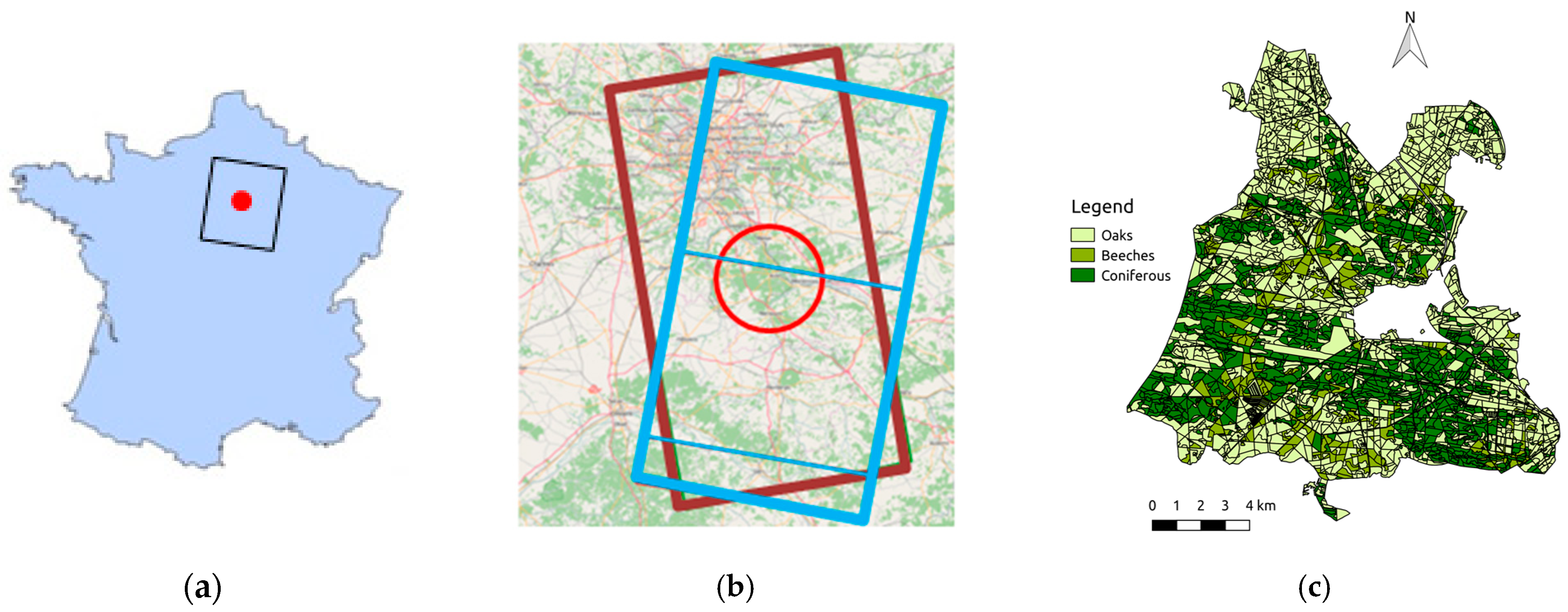
2.1. Study Site

The Fontainebleau Forest, located southeast of Paris (48°25′N, 2°40′E), is a large mixed deciduous-coniferous forest that extends over 17,000 ha (Figure 1). The region has a temperate climate with an average annual precipitation of 720 mm. The forest is managed by the French National Office for Forestry and is divided into multiple stands, each with an average area of about 5 ha. They are composed of single, mixed-deciduous, and mixed deciduous-coniferous species, and they include all the successional stages of stand development. Dominant species include oaks, beeches, and Scots pine. Most of the deciduous stands are located on flat topography, while most of the coniferous species are found on hilly topography and rocky soils. Deciduous trees have pronounced seasonality throughout the year, with the leaf-on stage beginning in April and the leaf-off stage beginning in November, and a growing period of about six months.

The site has been well-documented for decades as part of an experimental test site of the Ecologie Systématique et Evolution laboratory (ESE), which has collected many in situ data. In particular, air temperature, precipitation, and soil moisture in the upper soil layer (5 cm) are automatically recorded several times per hour. A flux tower was erected over a stand of oaks that is part of the Integrated Carbon Observatory System (ICOS) Ecosystem Thematic network [11]. More details about the Fontainebleau-Barbeau forest experimental site are available on http://www.barbeau.u-psud.fr/.

2.2. Sentinel-1 Data

Within the Copernicus Program, the ESA launched the Sentinel-1A and Sentinel-1B satellites in April 2014 and 2016, respectively. The two satellites have a six-day orbit cycle when considered together (12 days when considered individually), with each carrying identical SAR sensors onboard and operating in the C-band (λ = 5.6 cm, f = 5.4 GHz). The ESA has provided Sentinel-1A and -1B data since March 2015 and September 2016, respectively. The data are freely available on different web servers [12,13,14]. Over the main surfaces of the Earth, systematic acquisitions are made in the Interferometric Wide swath (IW) mode in dual VV and VH polarization. Across the 250 km-wide swath, incidence angles range from 29° (near range) to 46° (far range). For each acquisition, Ground Range Detected High Resolution (GRDH) and Single Look Complex (SLC) products were downloaded and used to derive σ⁰ (whose values are given in dB throughout this letter) and |ρ|, respectively. The characteristics of both products are summarized in

Table 1. Characteristics of Single Look Complex (SLC) and Ground Range Detected High Resolution (GRDH) products of the Interferometric Wide swathacquisition mode of Sentinel-1 satellites.

Acquisition Mode	Resolution (Range × Azimuth)	Pixel Spacing (Range × Azimuth)	Number of Looks
SLC	2.7 × 22 m to 3.5 × 22 m	2.3 × 14.1 m	1×1
GRDH	20 × 22 m	10 × 10 m	5×1

[15].

The Fontainebleau Forest is located at the intersection of ascending and descending orbits (relative no. 59 and 110, respectively) whose incidence angles range from 39–40°. Consequently, the temporal profiles shown over the different stands (Section 3.2) combine measurements acquired during both passes. Both the radar backscattering coefficient σ⁰ and the modulus of the interferometric coherence |ρ| were analyzed. After orthorectifying the passes [16], σ⁰ was extracted from the GRDH products using python scripts [17] implemented in QGIS software and based on Orfeo Toolbox Software [18]. These open-source tools, designed to process multiple Sentinel images automatically, can be used on a common PC (4 GB RAM) (A program to install the customized QGIS software in the Windows or Linux environments is available from http://remotesensing4all.net/index.php/en/2018/09/20/qgis-remote-sensing-kit-2/). Similar processing can be performed using the Sentinel Application Platform (SNAP) [19]. The Shuttle Radar Topographic Mission (SRTM) 1 arc second Digital Elevation Model (DEM), freely available on https://earthexplorer.usgs.gov/, was used for orthorectification processing.

After precise co-registration of two radar acquisitions at the sub-pixel level, the interferometric coherence between them is a complex number estimated for each pixel over a local neighborhood of N pixels, as follows:

$$\rho =\frac{{\sum }_{i=1}^N{z}_i·z_i^{\prime *}}{\sqrt{{\sum }_{i=1}^N{\left|z_i\right|}^2·{\sum }_{i=1}^N{\left|z_i^{\prime }\right|}^2}}=\left|\rho \right|e^{j\phi }$$

(1)

where z_i is the complex value of pixel i in the first acquisition, and $z_i^{\prime }$ is the corresponding complex value in the second acquisition.

Its absolute value |ρ|, called coherence, lies in the range of [0, 1]. It characterizes the geometric stability, at a wavelength scale, of the elementary scatterers within a resolution cell. It is low over dense vegetation (in which elementary scatterers, i.e., leaves and twigs, move with weather events, i.e., rain and wind) and high over solid bare soils, such as rocky soils. Coherence was estimated from SLC data over a 11 × 3 local neighborhood (i.e., N = 33 in rel. 1), yielding an approximately square area of ground (~42 × 44 m). A tutorial to calculate the interferometric coherence from IW SLC products with SNAP software is available in [20].

2.3. Landsat-8 Data

To analyze the sensitivity of radar data to vegetation phenology, radar temporal profiles were compared to the Normalized Difference Vegetation Index (NDVI) derived from bands 4 and 5 of the Landsat-8 optical Operational Land Imager (OLI) sensor. This sensor has a 180 km-wide swath, covering the globe every 16 days, and the spatial resolution associated with bands 4 and 5 is 30 m. Many studies have demonstrated the sensitivity of NDVI to photosynthetic green materials in the vegetation canopy. Consequently, NDVI is widely used for monitoring vegetation phenology. To correct atmospheric perturbations (which decrease NDVI values recorded from the top of the canopy), a maximum-value filter over a 48-day period (i.e., three consecutive acquisitions) was used.

3. Results and Discussion

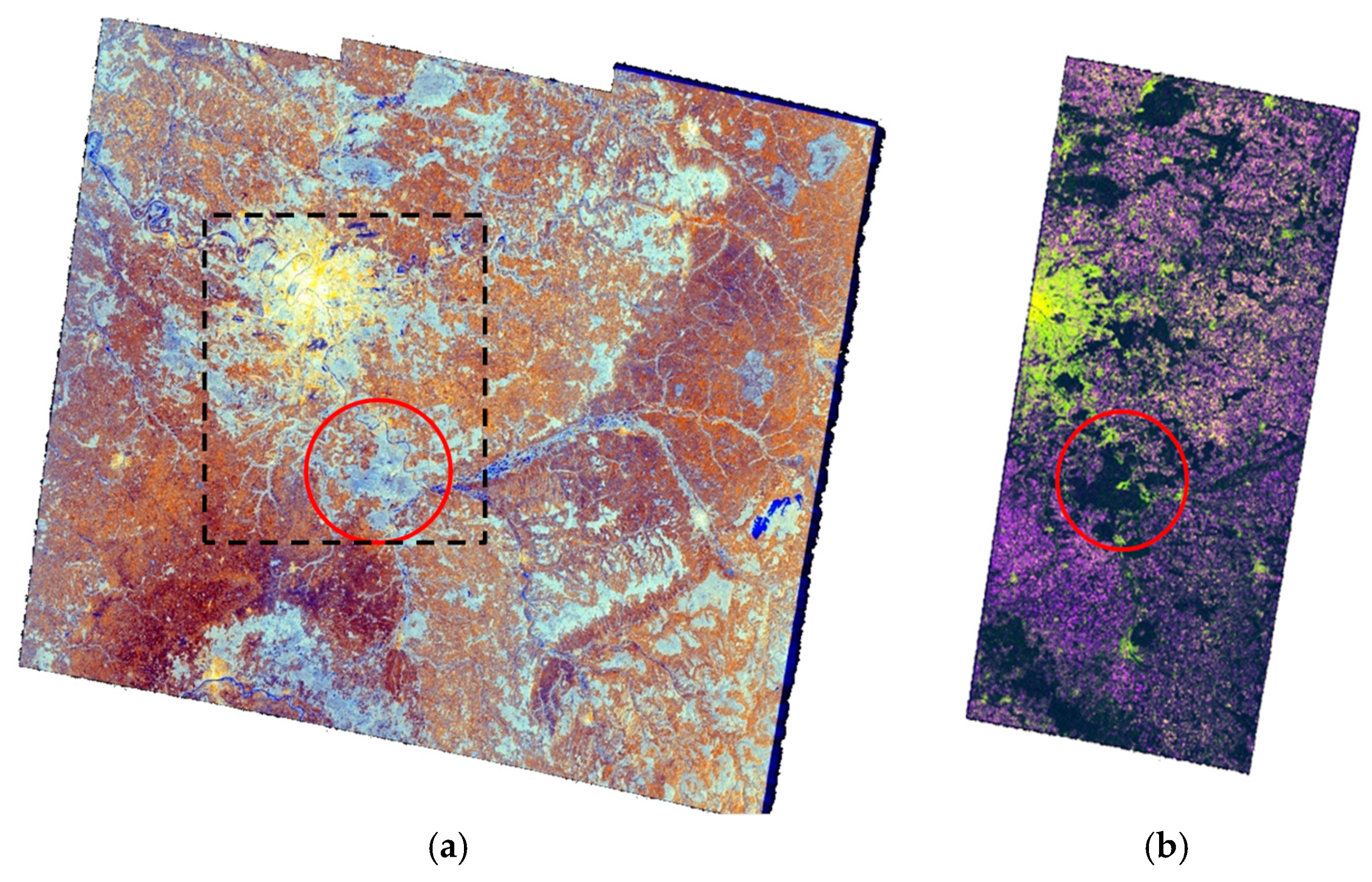
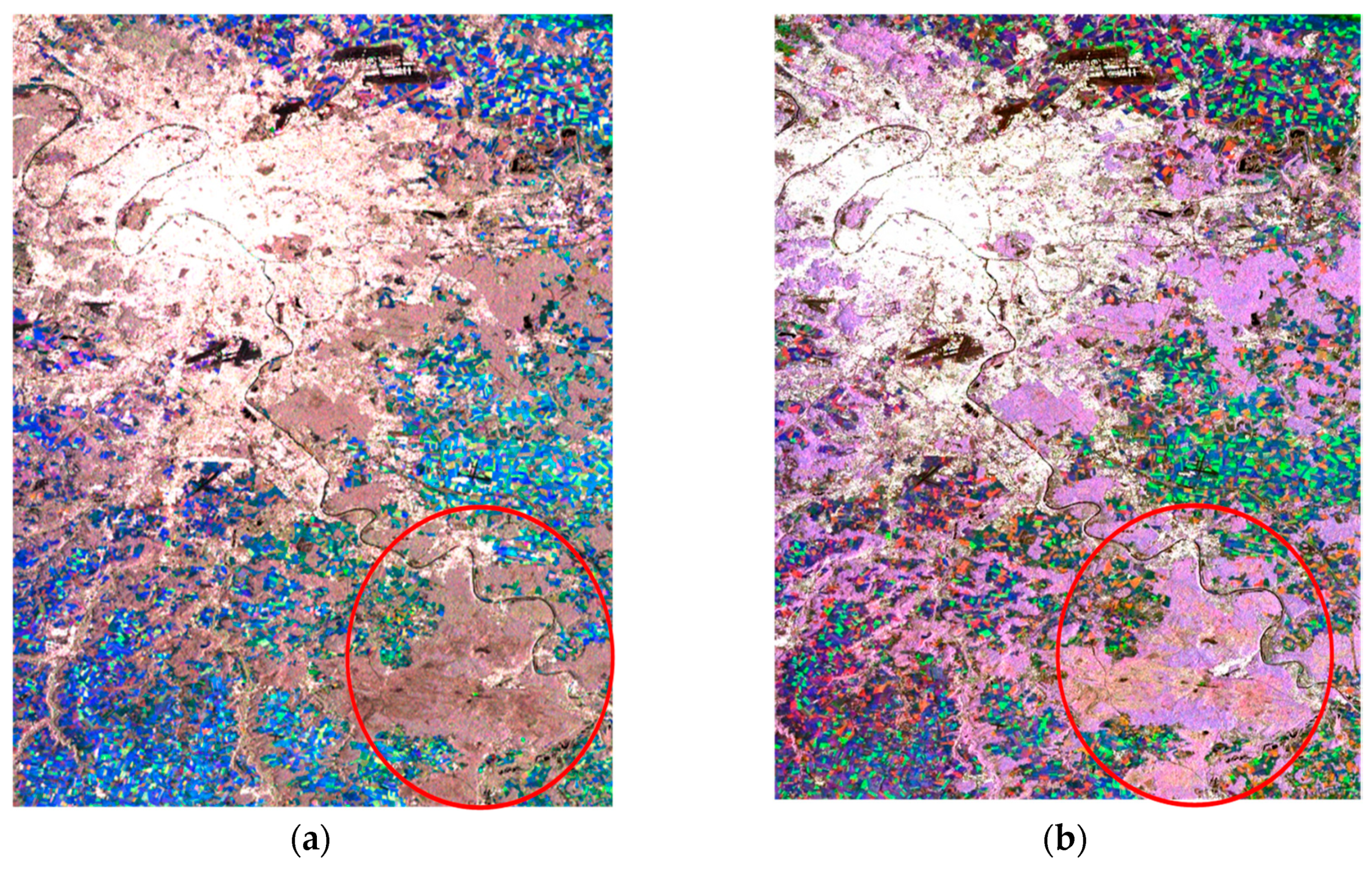
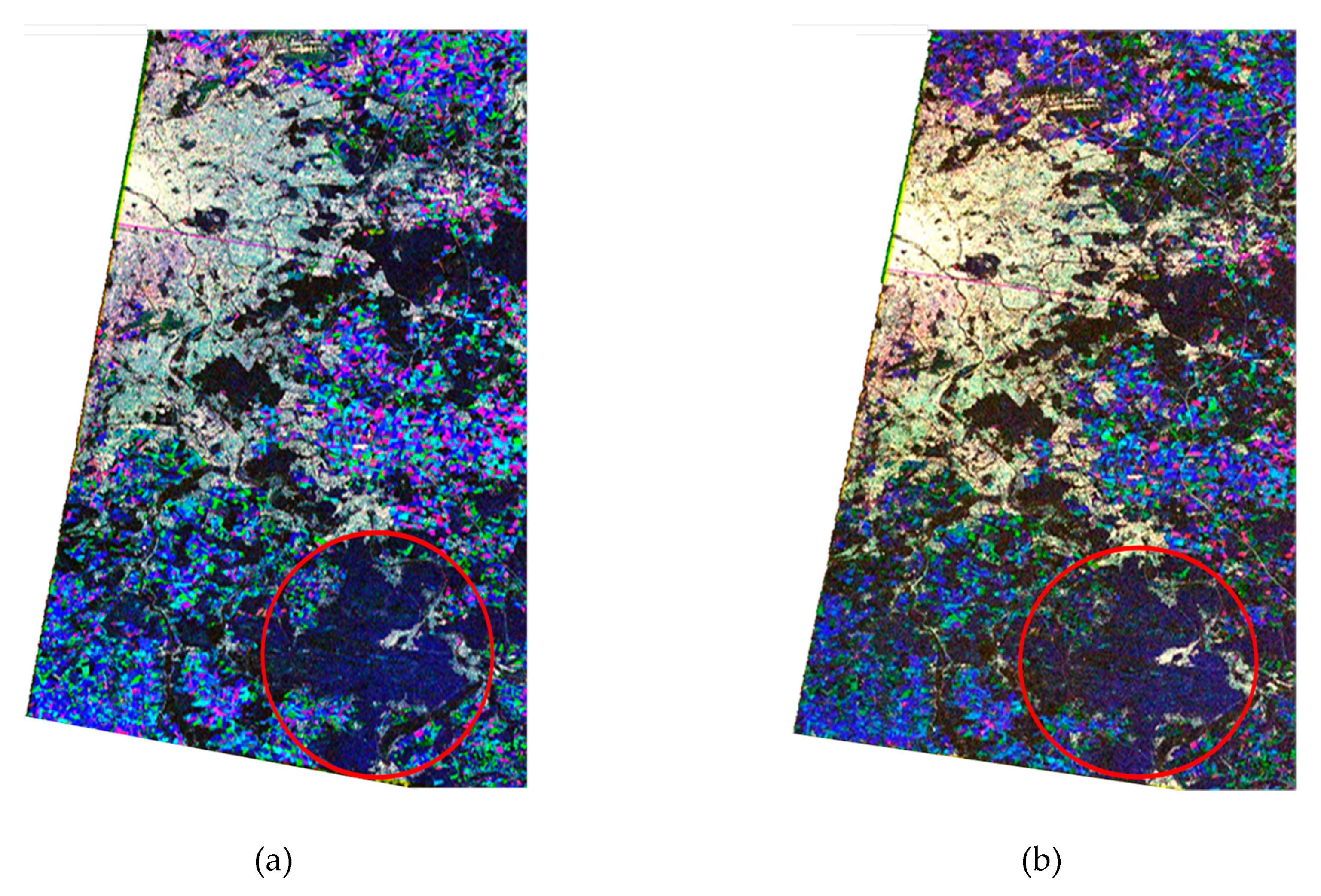
3.1. Spatio-Temporal Analysis

Figure 2 shows two color-composite images in several polarizations over the Ile de France region for σ⁰ (R: ${\sigma }_{VV}^0$, G: ${\sigma }_{VH}^0$, B: ${\sigma }_{VH}^0/{\sigma }_{VV}^0$) and |ρ| (R: $\left|{\rho }_{VV}\right|$, G: $\left|{\rho }_{VH}\right|$, B: $\left|{\rho }_{VV}\right|$/$\left|{\rho }_{VH}\right|$), respectively. The σ⁰ image shows three sub-swaths of the IW mode (Figure 2a), while that for |ρ| shows only the second sub-swath (Figure 2b). Urban, agricultural, and forested areas are clearly distinguished in both images. Urban areas, such as Paris, appear in bright white-yellow tones in both images, indicating high σ⁰ and |ρ| values for each polarization. In the σ⁰ image (Figure 2a), water appears blue due to relatively low ${\sigma }_{VV}^0$ and ${\sigma }_{VH}^0$ values and consequently high ${\sigma }_{VH}^0/{\sigma }_{VV}^0$ values (~1). Agricultural areas appear in brown tones due to higher ${\sigma }_{VH}^0$ values (in March they appear as areas with low vegetation or bare soils), while forested areas appear in cyan due to high values of both ${\sigma }_{VH}^0$ and ${\sigma }_{VH}^0/{\sigma }_{VV}^0$. As expected, in the coherence image (Figure 2b), forested and water areas are dark due to low |ρ| values observed in each polarization. Agricultural areas are more variable, with purple and yellow tones that denote different behaviors of the coherence in VV and VH polarizations depending on the state of a field’s surface.

Figure 3 shows a temporal color composite of σ⁰ images (R: 5 May, G: 2 September, B: 19 December 2015) with VV and VH polarization (Figure 3a,b, respectively). Forested and urban areas appear as gray tones, especially with VV polarization, indicating relatively low temporal variations. More pronounced colors are observed over the Fontainebleau Forest with VH polarization, indicating higher temporal variations than those with VV polarization. In contrast, agricultural fields show a variety of saturated colors, indicating multiple distinct temporal variations, depending on crop type and agricultural practice.

The spatio-temporal behavior of |ρ| over the same region is illustrated with VV and VH polarizations (Figure 4a,b, respectively) for three acquisition pairs in 2015 (05–17 May, 02–14 September, and 19–31 December). Since only Sentinel-1 was operational during this period, the temporal revisit time between two consecutive acquisitions was 12 days. Both polarizations have similar patterns: white and dark colors over urban and forested areas, respectively, at both polarizations indicate that these areas have stable spatio-temporal behavior. For σ⁰, agricultural areas have high saturated colors, i.e., distinct spatio-temporal variations.

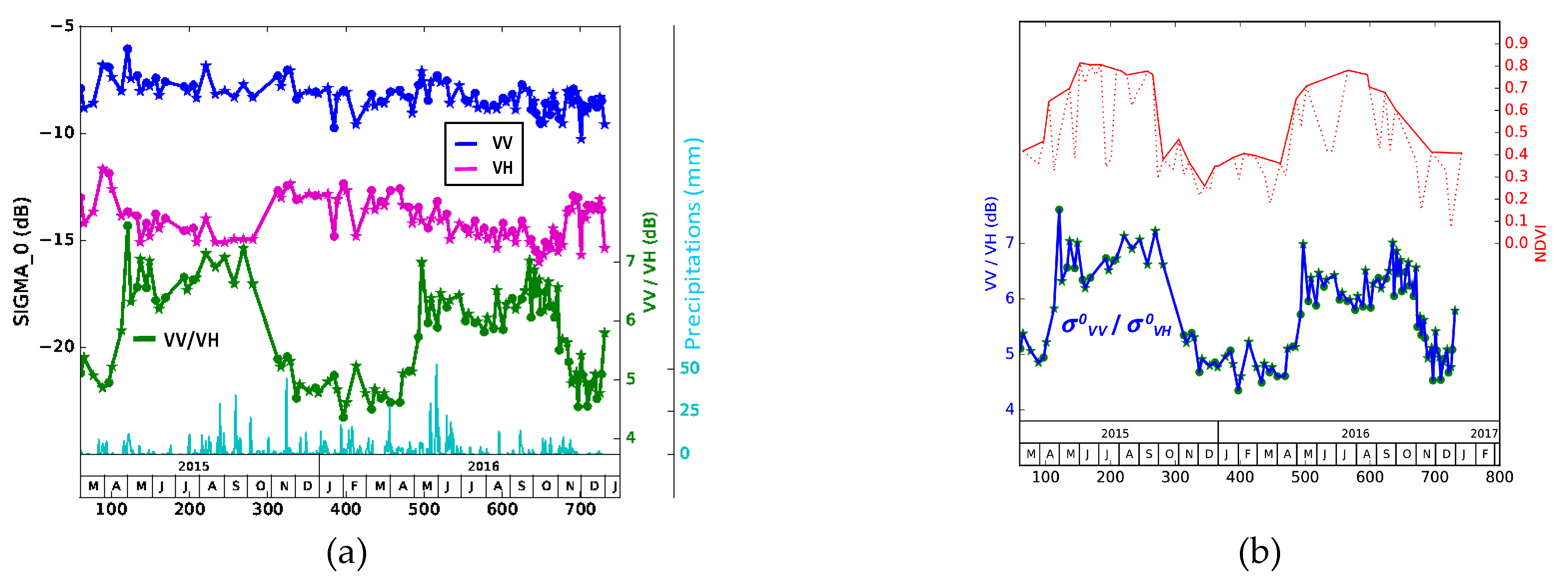
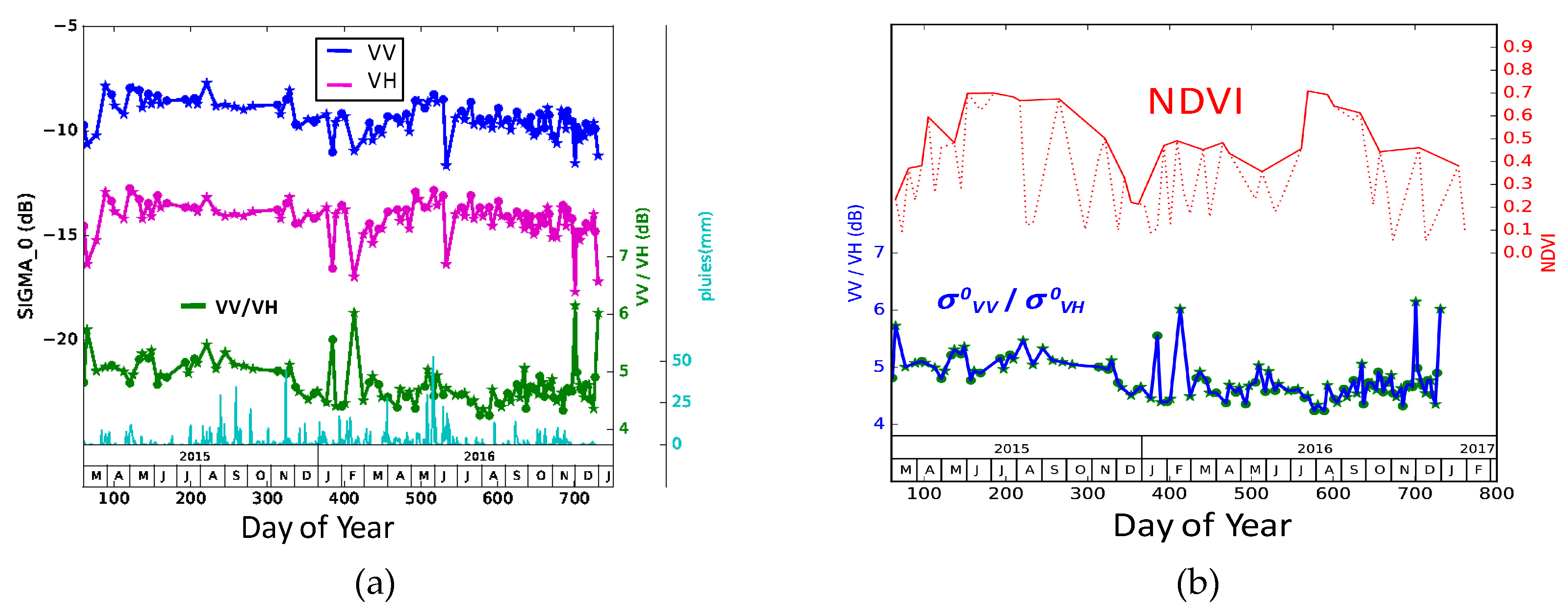
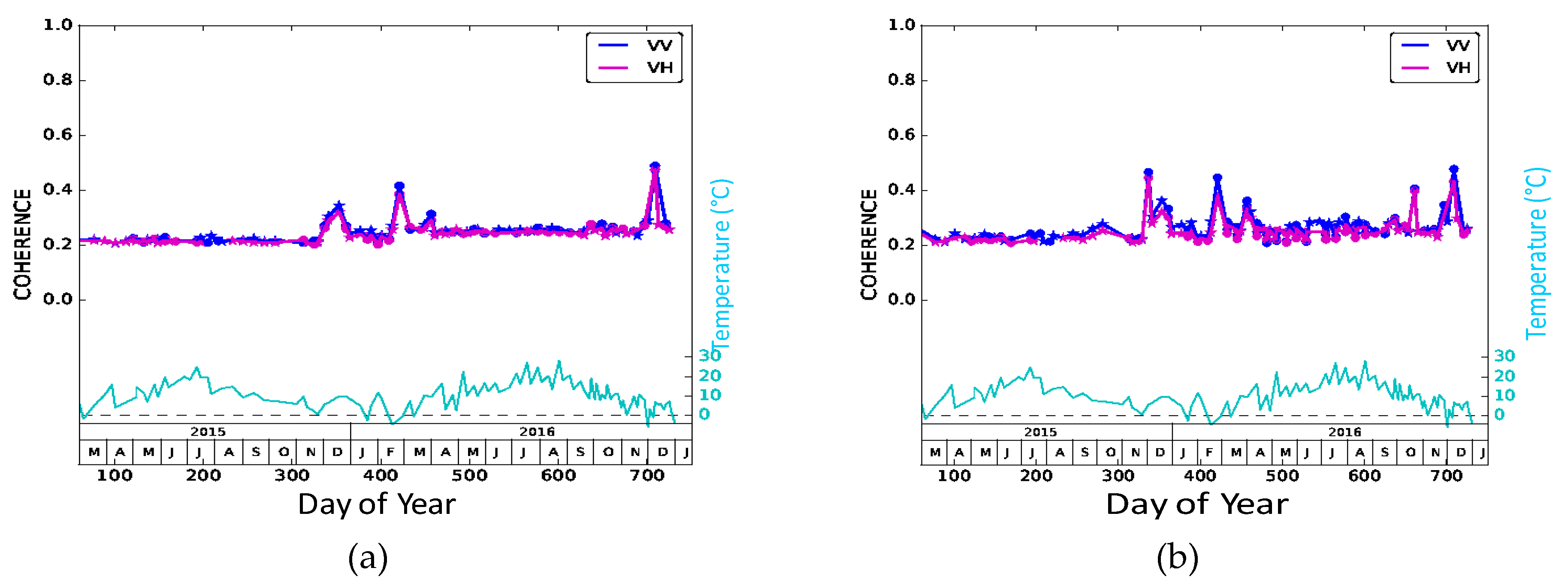
3.2. Temporal Profile Analysis

To further analyze the temporal behavior of Sentinel-1 data over temperate forests, temporal profiles were extracted from March 2015 to December 2017 over different stands. On the whole, two main different classes of temporal signatures could be observed, depending on whether the species were deciduous or coniferous. We show here the temporal behavior observed over one mature stand of deciduous (oaks) and one mature stand of pine trees, which are representative of both classes. Figure 5 shows temporal profiles of σ⁰ over the oak stand. Each point corresponds to the mean σ⁰ of all pixels (~10,500) in each image of the stand. As previously observed 10], and unlike observations of bare soils over areas with little vegetation [21,22,23], we did not observe any direct relation between precipitation (or cumulative precipitation, or in situ soil moisture, not shown) and σ⁰ profiles. This is due to the difference between recorded precipitation and the precipitation that trees intercept, which would greatly influence the radar signal over forested areas.

As already shown by [10], no seasonal variation is observed with VV polarization (blue profile), while slight variations are visible in the ${\sigma }_{VH}^0$ temporal profile. An overall slight decrease (around 1 dB) is observed for both polarizations over the whole period, which is unexplained for now. This variation does not come from drift in Sentinel-1 SAR calibration, as both S1-A and S1-B sensors show stable behaviour (+/−0.3 dB) since the end of their commissioning phases [24].

In contrast, distinct seasonality is observed for the ${\sigma }_{VV}^0/{\sigma }_{VH}^0$ ratio (green profile), which increases in spring (April–May) and decreases in autumn (September–October), with an annual amplitude of about 3 dB (range = 4–7 dB). The temporal signature of the ${\sigma }_{VV}^0/{\sigma }_{VH}^0$ ratio appears to coincide temporally with the NDVI profile derived from Landsat-8 OLI (Figure 5b), with a correlation coefficient value of r = 0.77 and a p-value of 9.10⁻⁷. This confirms the sensitivity of the C-band to the upper leaves and stems of forest canopies. This temporal profile behavior results from the decrease in ${\sigma }_{VH}^0$ in spring (from −12.5 to −15 dB), while ${\sigma }_{VV}^0$ remains relatively constant. Further investigations based on a radiative transfer model [25] are currently being performed in order to better understand the physics behind these observations.

This figure is a striking illustration of the potential of the Sentinel-1 IW mode for identifying vegetation phenology at the local scale. The double polarization configuration, combined with a six-day revisit time with 20 m of spatial resolution, makes this mission the first radar mission particularly well-suited for monitoring seasonal variations in vegetation. This kind of monitoring was impossible with ERS-1 SAR, which acquired radar data in the C-band with only VV polarization and an overly large repeat cycle (35 days) [10].

The temporal profile over a pine stand (corresponding to about 6500 Sentinel-1 pixels) is shown in Figure 6. Isolated measurements that appear as outliers in the σ⁰ profiles are distinguished (e.g., ${\sigma }_{VV}^0/{\sigma }_{VH}^0$ values in January or February 2016). These values are due to calibration problems, which occurred for several acquisitions. The data are still under investigation by using the ESA support service. No distinct seasonal cycle is observed over these coniferous tree stands. Slight variations are observed for ${\sigma }_{VV}^0/{\sigma }_{VH}^0$, with an annual amplitude less than 1 dB, which are difficult to interpret in relation to environmental variables. In contrast, the NDVI profile shows distinct seasonality that results mainly from the understory, which is composed of deciduous species (i.e., grasses, ferns, and shrubs). In this case, optical data pointing at the nadir are sensitive to it, while radar data, acquired at about 40° of the incidence angle, are mainly sensitive to the pine canopy.

Figure 7 shows temporal signatures of the coherence |ρ| over the oak stand and the pine stand. The coherence remains low and stable for both stands, apparently corresponding to noise (|ρ| = 0.2). This is not surprising for such types of mature vegetation. For both stands, the coherence increases during winter (from November to February). These higher values could be due to the low temperatures causing stems and needles to stiffen (though they did not freeze). The observed behavior appears erratic, and has eluded interpretation to date.

5. Conclusions

Sentinel-1 data were analyzed for a temperate forest located near Paris, France. Two parameters were analyzed: the backscattering coefficient σ⁰, and the coherence|ρ|. Over the entire Ile de France region, σ⁰ appeared stable over urban areas and showed large spatio-temporal variations over agricultural areas. Over the forest, ${\sigma }_{VV}^0$ appeared relatively stable, while ${\sigma }_{VH}^0$ had more pronounced variations. The coherence |ρ| had similar behavior to both VV and VH polarizations, and appeared stable over urban areas and forests but had distinct spatio-temporal variations over agricultural areas. Analysis of temporal signatures over deciduous (oaks) and coniferous (pines) stands showed distinct seasonality (with an annual amplitude of about 3dB) observed for the ${\sigma }_{VV}^0/{\sigma }_{VH}^0$ ratio over the oak stand. The similarity between ${\sigma }_{VV}^0/{\sigma }_{VH}^0$ and NDVI derived from the Landsat-8 OLI sensor confirms the sensitivity of the C-band to leaves and stems in the upper canopy. In contrast, no clear seasonal variations were visible over the pine stand, even for ${\sigma }_{VV}^0/{\sigma }_{VH}^0$. The coherence |ρ| remained stable, with low values (|ρ| = 0.2) from March to November, and higher values from November to February, which were more difficult to interpret.

This study showed the strong potential of Sentinel-1 for monitoring temperate forests. For the first time, systematic acquisitions with the same configurations every six days (in Europe), combined with dual polarization acquisitions, make these data particularly well-suited for monitoring deciduous forest phenology, in particular by using the ratio between VV and VH radar backscattering coefficients. It opens up new perspectives concerning vegetation monitoring with SAR sensors by allowing for the monitoring of the phenology independently of the cloud cover, and moreover, future studies based on electromagnetic models will allow assessment of whether quantitative variables, such as leaf biomass, can be estimated from Sentinel-1 data. These studies will also allow determination of the optimal configuration, with respect to frequency, polarization, and incidence angles, for the accurate estimation of phonological stages in order to specify future SAR sensor specifications.

References

1. Justice, C.O.; Townshend, J.R.G.; Holben, B.N.; Tucker, C.J. Analysis of the phenology of global vegetation using meteorological satellite data. Int. J. Remote Sens. 1985, 8, 1271–1318. [Google Scholar] [CrossRef]
2. Hansen, M.; Potapov, P.V.; Moore, R.; Hancher, M.; Turubanova, S.A.; Tyukavina, A.; Thau, D.; Stehman, S.V.; Goetz, S.J.; Loveland, T.R.; et al. High-resolution global maps of 21st-century forest cover change. Science 2013, 342, 850–853. [Google Scholar] [CrossRef] [PubMed]
3. Zhang, X.; Friedl, M.A.; Schaaf, C.B.; Strahler, A.H.; Hodges, J.C.F.; Gao, F.; Reed, B.C.; Huete, A. Monitoring vegetation phenology using MODIS. Remote Sens. Environ. 2003, 84, 471–475. [Google Scholar] [CrossRef]
4. Keenan, T.F.; Gray, J.; Fried, L.M.A.; Toomey, M.; Bohrer, G.; Hollinger, D.Y.; Munger, J.W.; O’Keefe, J.; Schmid, H.P.; Wing, I.S.; et al. Net carbon uptake has increased through warming-induced changes in temperate forest phenology. Nat. Clim. Chang. 2014, 4, 598–604. [Google Scholar] [CrossRef]
5. Chmielewski, F.M.; Rötzer, T. Response of tree phenology to climate change across Europe. Agric. For. Meteorol. 2001, 108, 101–112. [Google Scholar] [CrossRef]
6. Kramer, K.; Leinonen, I.; Loustau, D. The importance of phenology for the evaluation of impact of climate change on growth of boreal, temperate and Mediterranean forests ecosystems: An overview. Int. J. Biometeorol. 2000, 44, 67–75. [Google Scholar] [CrossRef] [PubMed]
7. Frison, P.-L.; Mougin, E. Monitoring global vegetation dynamics with ERS-1 wind scatterometer data. Int. J. Remote Sens. 1996, 17, 3201–3218. [Google Scholar] [CrossRef]
8. Frison, P.-L.; Paillou, P.; Sayah, N.; Pottier, E.; Rudant, J.-P. Spatio-temporal monitoring of evaporitic processes using multi-resolution C-band radar remote sensing: Example of the Chott el Djerid, Tunisia. Can. J. Remote Sens. 2013, 39, 127–137. [Google Scholar] [CrossRef]
9. Wooding, M.G.; Zmuda, A.D.; Griffiths, G.H. Crop discrimination using multi-temporal ERS-1 SAR data. In Proceedings of the 2nd ERS-1 Symposium, Hamburg, Germany, 11–14 October 1993; pp. 51–56. [Google Scholar]
10. Proisy, C.; Mougin, E.; Dufrêne, E.; Le Dantec, V. Monitoring seasonal changes of a mixed temperate forest using ERS SAR observations. IEEE Trans. Geosci. Remote Sens. 2000, 38, 540–552. [Google Scholar] [CrossRef]
11. ICOS Ecosystem Thematic Center. Available online: www.europe-fluxdata.eu/icos (accessed on 7 September 2018).
12. Copernicus Open Data Hub. Available online: https://scihub.copernicus.eu (accessed on 7 September 2018).
13. PEPS—French Access to the Sentinel Products. Available online: https://peps.cnes.fr/rocket/#/home (accessed on 7 September 2018).
14. Alaska Satellite Facility. Available online: https://www.asf.alaska.edu/sentinel/data (accessed on 7 September 2018).
15. Sentinel-1 SAR Technical Guide. Available online: https://sentinel.esa.int/web/sentinel/technical-guides/sentinel-1-sar (accessed on 7 September 2018).
16. Small, D. Flattening gamma: Radiometric terrain correction for SAR imagery. IEEE Trans. Geosci. Remote Sens. 2011, 49, 3081–3093. [Google Scholar] [CrossRef]
17. Frison, P.-L.; Lardeux, C. Vegetation cartography from Sentinel-1 radar images. In QGIS and Application in Agriculture and Forest; Baghdadi, N., Mallet, C., Zribi, M., Eds.; ISTE Press Ltd.: London, UK; Elsevier Ltd.: Oxford, UK, 2017; pp. 181–214. ISBN 978-1786301888. [Google Scholar]
18. OrfeoToolBox. Available online: https://www.orfeo-toolbox.org (accessed on 7 September 2018).
19. STEP Science Toolbox Exploitation Platform: SNAP. Available online: http://step.esa.int/main/toolboxes/snap (accessed on 7 September 2018).
20. Meyer, F.J. Sentinel-1 InSAR Processing Using the SNAP Toolbox. Available online: https://media.asf.alaska.edu/uploads/pdf/s-1tbx_insar_recipe_6-16-17_final.pdf (accessed on 8 November 2018).
21. Zribi, M.; Saux-Picart, S.; André, C.; Descroix, L.; Ottlé, C.; Kallel, A. Soil moisture mapping based on ASAR/ENVISAT radar data over a Sahelian region. Int. J. Remote Sens. 2007, 28, 3547–3565. [Google Scholar] [CrossRef]
22. Baghdadi, N.; El Hajj, M.; Zribi, M.; Fayad, I. Coupling SAR C-band and optical data for soil moisture and leaf area index retrieval over irrigated grasslands. IEEE J. Sel. Top. Appl. Earth Obs. Remote Sens. 2016, 9, 1129–1244. [Google Scholar] [CrossRef]
23. Baup, F.; Mougin, E.; de Rosnay, P.; Timouk, F.; Chênerie, I. Surface soil moisture estimation over the AMMA Sahelian site in Mali using ENVISAT/ASAR data. Remote Sens. Environ. 2007, 109, 473–481. [Google Scholar] [CrossRef] [Green Version]
24. CLS, S1-A N-Cyclic Performance Report—2018-06. Technical Report, October 2018. Available online: https://sentinel.esa.int/web/sentinel/user-guides/sentinel-1-sar/document-library (accessed on 29 November 2018).
25. Karam, M.A.; Fung, A.K.; Lang, R.H.; Chauhan, N.S. A microwave scattering model for layered vegetation. IEEE Trans. Geosci. Remote Sens. 1992, 30, 767–784. [Google Scholar] [CrossRef] [Green Version]
Figure 1. (a) Overall location of Fontainebleau area in France with the coverage resulting from Sentinel-1 descending orbit; (b) zoom in on the Fontainebleau Forest with the coverages from ascending (brown rectangle) and descending (blue rectangle) Sentinel-1 acquisitions (relative orbits no. 59 and 110, respectively); (c) inventory of tree species in the Forest’s stands. Colors indicate the dominant species.
Remotesensing 10 02049 g001
Figure 2. (a) Multi-polarization color-composite of the radar backscattering coefficient σ0 image acquired on 18 March 2015: R: σ V V 0 , G: σ V H 0 , B: σ V H 0 / σ V V 0 ; (b) coherence derived from the 18–30 March 2015 acquisitions of the second sub-swath: R: | ρ V V | , G: | ρ V H | , B: | ρ V V | / | ρ V H | . The red circle corresponds to the Fontainebleau Forest. Paris is the bright feature in white-yellow, northwest of Fontainebleau. The dashed rectangle corresponds to the area shown in Figure 3.
Remotesensing 10 02049 g002
Figure 3. Temporal color-composite σ0 image, (R: 05/05/2015, G: 02/09/2015, B: 19/12/2015) (a) VV polarization; (b) VH polarization. The area corresponds to the dashed rectangle in Figure 2. The red circle corresponds to the Fontainebleau Forest.
Remotesensing 10 02049 g003
Figure 4. Temporal color-composite |ρ| image, (R: 5–17 May, G: 02–14 Sept., B: 19–31 Dec. 2015).(a) VV polarization; (b) VH polarization. The red circle corresponds to the Fontainebleau Forest.
Remotesensing 10 02049 g004
Figure 5. Temporal profiles of σ0 observed over an oak stand. (a) σ V V 0 , σ V H 0 , and σ V V 0 / σ V H 0 are represented in blue, magenta, and green, respectively. In situ precipitation is also shown (cyan); ascending and descending passes measurements are plotted as “•” and “*”, respectively. (b) Landsat-8 Operational Land Imager (OLI)-derived Normalized Difference Vegetation Index (NDVI) (-- raw data; — maximum value over a sliding 48-day period) overlaid on σ V V 0 / σ V H 0 signatures.
Remotesensing 10 02049 g005
Figure 6. Temporal profile of σ0 observed over a pine stand. (a) σ V V 0 , σ V H 0 , and σ V V 0 / σ V H 0 are represented in blue, magenta, and green, respectively. In situ precipitation is also shown (cyan); ascending and descending passes measurements are plotted as “•” and “*”, respectively. (b) Landsat-8 OLI-derived NDVI (-- raw data; — maximum value over a sliding 48-day period) overlaid on σ V V 0 / σ V H 0 signatures.
Remotesensing 10 02049 g006
Figure 7. Temporal profiles of |ρ| observed over an oak (a) and a pine (b) stand with VV and VH polarization. In situ temperatures at 2 m are also shown (cyan).
Remotesensing 10 02049 g007