Convolutional Neural Network Based Multipath Detection Method for Static and Kinematic GPS High Precision Positioning


Abstract
:1. Introduction
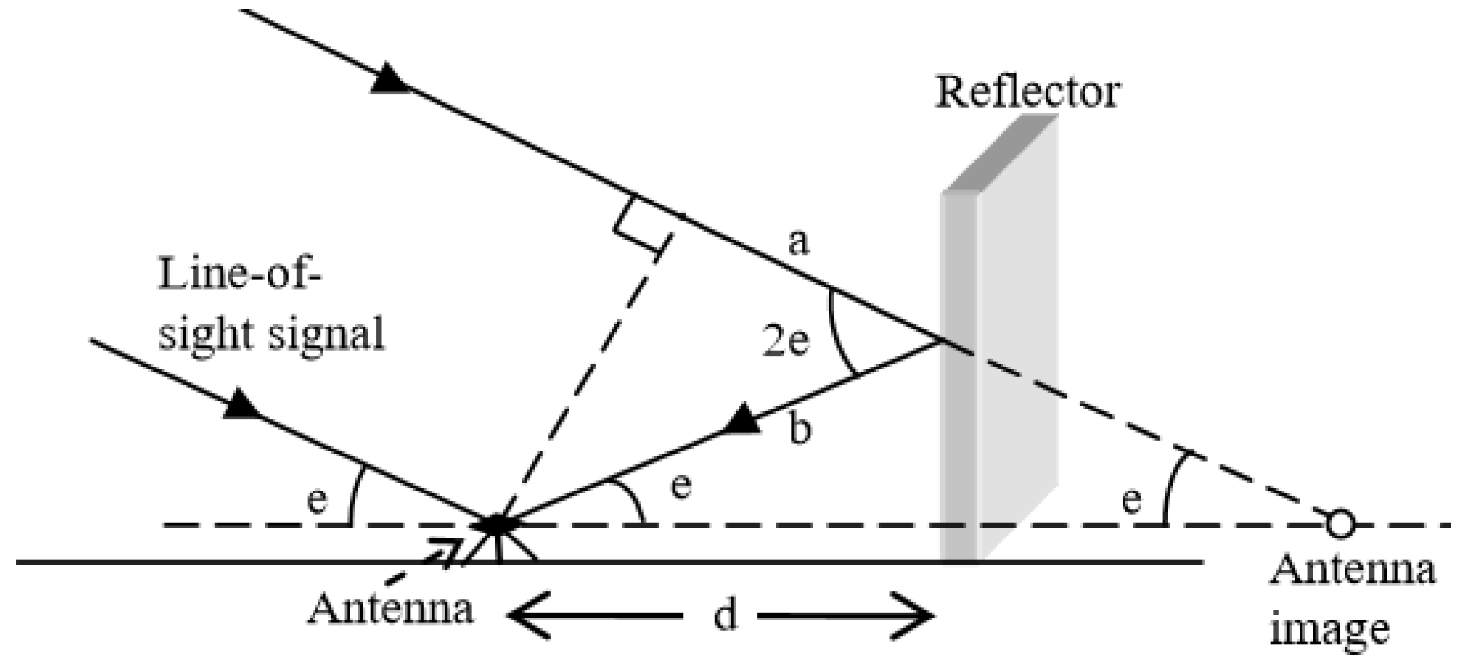
1.1. Introduction of GPS Multipath Error and Its Mitigation
1.2. Introduction of Relevant Machine Learning Algorithms
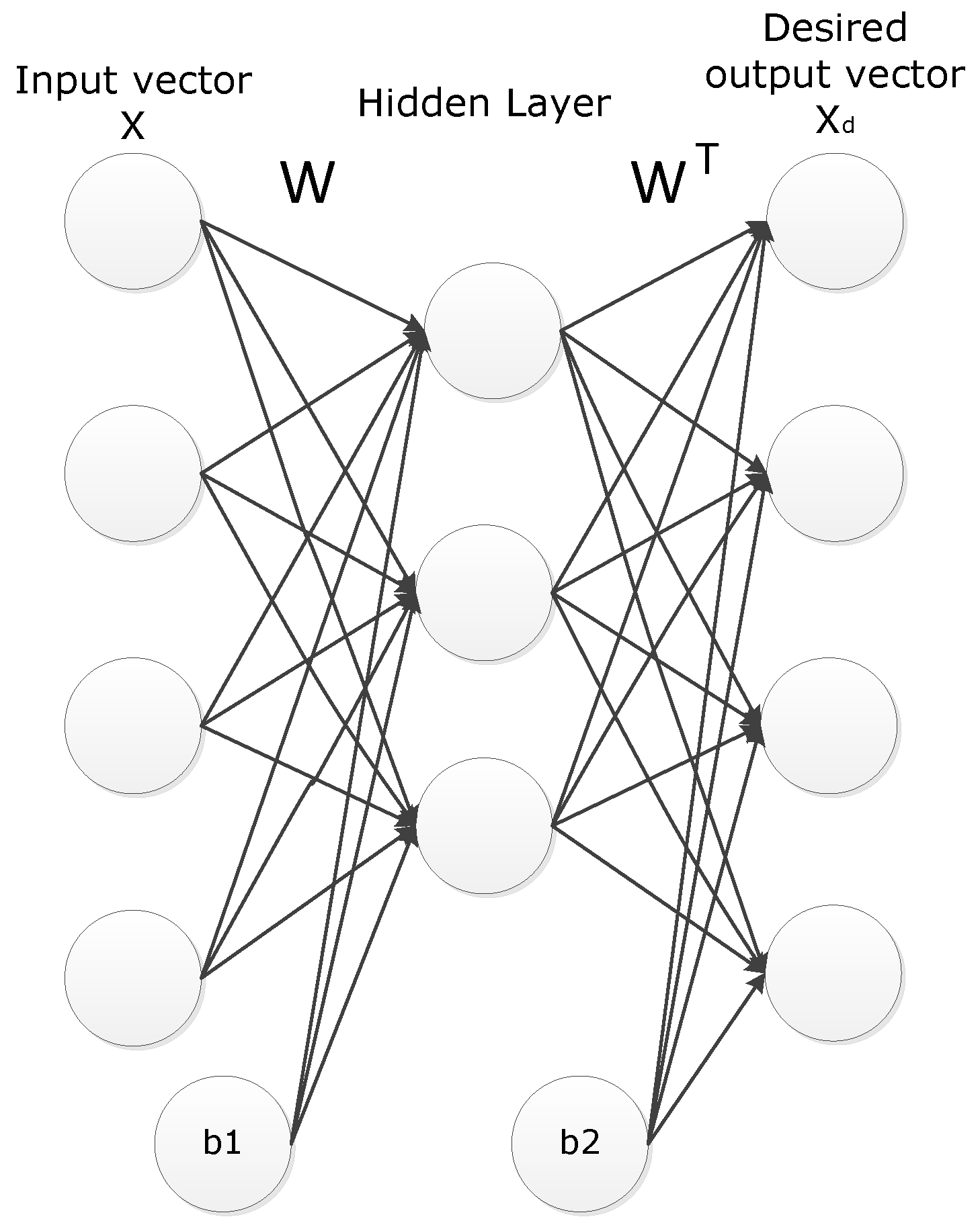
2. Proposed Convolutional Neural Network Based Multipath Detection Method
- Pre-process each in the time window (i.e. Table 1) to by:
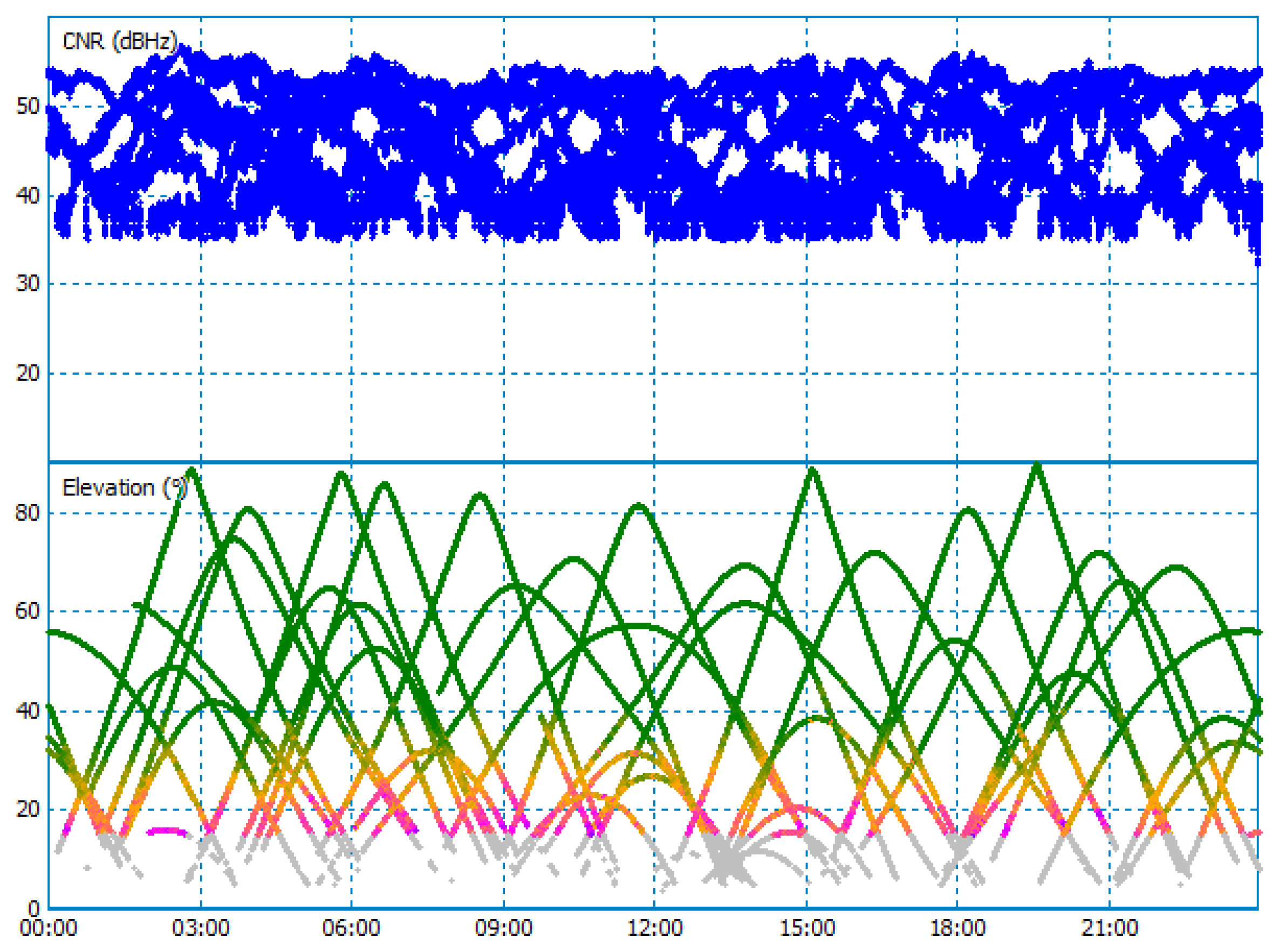
- Scale the and to [0.1] using the following two equations:where and are scaled and from Table 1, respectively; is the sigmoid function defined in Equation (4). and are the upper and lower bounds of CNR in all measurements (not just in the time window). This step as data pre-processing (scaling all the input data to [0, 1]) is compulsory because sigmoid function, i.e., Equation (4), is used when training SAE in Step 3. The sigmoid function has an output range of [0, 1]. As described in Section 1, an SAE neural network has identical input and output values, so the input values of SAE need to be restricted to [0, 1] as well. The values of and are set as 60 and 30 in this research because this range covers most of the observed CNR in the direct-signal only and multipath contaminated data. An example plot of CNR in 24 h is shown in Figure 3. Unlike CNR, MP is not bounded, the logarithmic function is used in Equation (9) to scale to the range within activation range of sigmoid function, and then sigmoid function is used to make sure is within [0, 1]. can assure that has a consistent positive or negative sign with .
- If the detector is untrained, convolution filters are trained for MP and CNR by SAE, respectively. The training is implemented in minFunc, developed by Schmidt [30]. After tuning, the parameters for convolution filters used in this work are: the number of filters = 4, the length of each filter = 5, which proved to give best performance (more detail is presented in Section 5).
- Using Equations (3) and (4) to compute the feature activations of each filter throughout the network in the convolution layer.
- In the pooling layer, the feature maps are subsampled to reduce data resolution. The determination of subsampling factor is presented in Section 5.
3. Validation Methodologies of the Proposed Method
- The proposed method aims to detect multipath errors in carrier phase measurements (not signals). The multipath errors in measurements are the output of processed signals from receiver hardware. Therefore, the multipath errors to be detected in carrier-phase measurements are the results of the combination of antenna architecture and receiver signal processing architecture (including correlator design). Characteristics of multipath errors in carrier phase measurements of combinations of antennas and receivers are very similar. Factors affecting the phases and magnitudes of carrier phase multipath errors can be found in [3].
- The proposed method aims to detect multipath errors. The definition of multipath errors is described in Section 1.1 and [3]. Non-line-of-sight only measurements are not multipath contaminated measurements; therefore, the non-line-of-sight only problem is outside the scope of this investigation.
- The proposed method doesn’t rely on the repeated multipath characteristics in sidereal days, and doesn’t need multipath pattern/signature to build up in the previous consecutive measurement epochs in real-time implementation of the multipath detection. A machine learning classifier can learn the characteristics of multipath errors in carrier phase measurements from CNR and MP data in the training datasets as described in Section 2.
4. Data Description
4.1. Description of Data Simulation and Collection
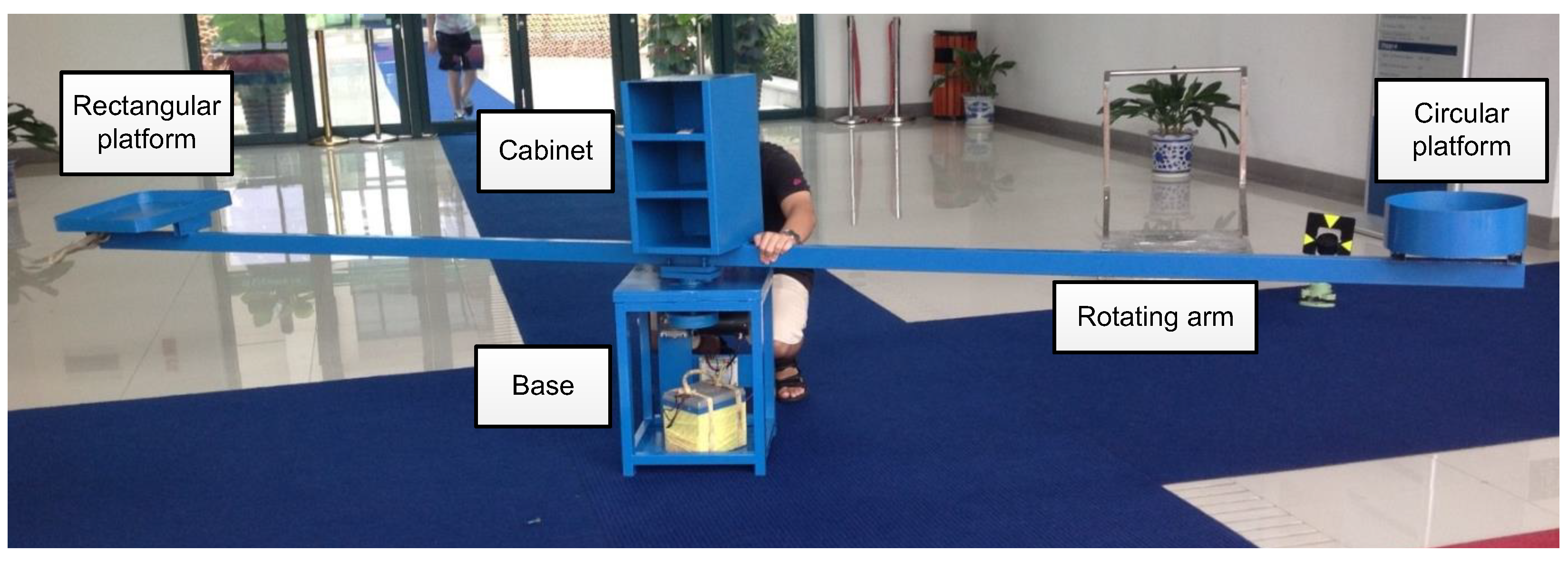
4.2. Description of Real Data Collection
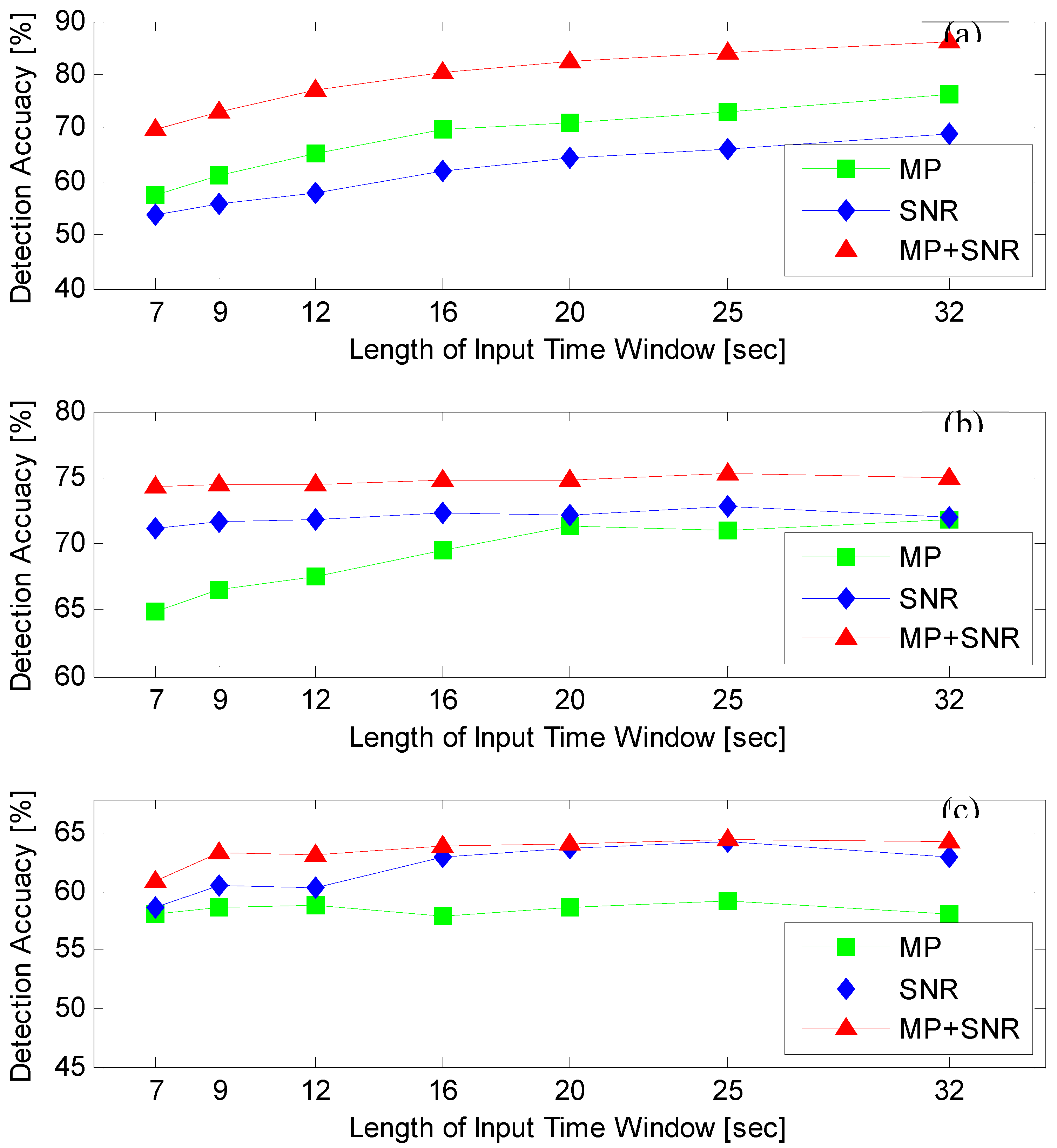
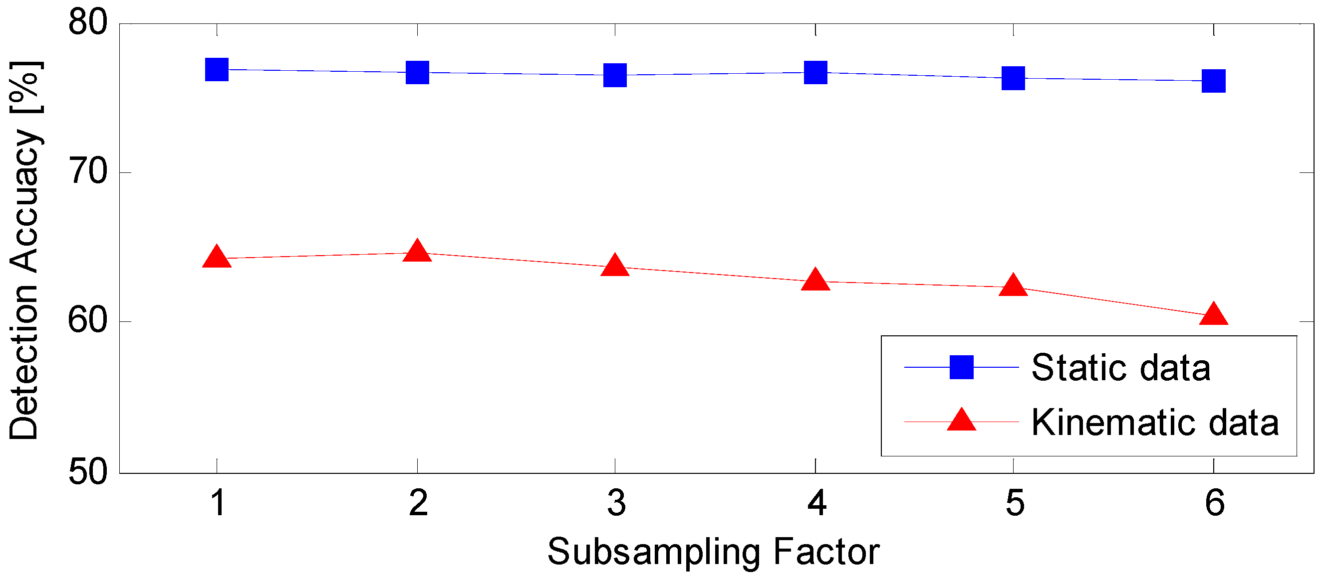
5. Tuning of Parameters and Comparison between Classifiers
6. Test Results
7. Conclusions
Author Contributions
Funding
Acknowledgments
Conflicts of Interest
References
- Lau, L.; Cross, P.; Steen, M. Flight Tests of Error-Bounded Heading and Pitch Determination with Two GPS Receivers. IEEE Trans. Aerosp. Electron. Syst. 2012, 48, 388–404. [Google Scholar] [CrossRef]
- Bhatt, D.; Aggarwal, P.; Devabhaktuni, V.; Bhattacharya, P. A novel hybrid fusion algorithm to bridge the period of GPS outages using low-cost INS. Expert Syst. Appl. 2014, 41, 2166–2173. [Google Scholar] [CrossRef]
- Lau, L.; Cross, P. Development and testing of a new ray-tracing approach to GNSS carrier-phase multipath modelling. J. Geodesy 2007, 81, 713–732. [Google Scholar] [CrossRef]
- Phan, Q.H.; Tan, S.L.; McLoughlin, I. GPS multipath mitigation: A nonlinear regression approach. GPS Solut. 2013, 17, 371–380. [Google Scholar] [CrossRef]
- Phan, Q.H.; Tan, S.L.; McLoughlin, I.; Vu, D.L. A unified framework for GPS code and carrier-phase multipath mitigation using support vector regression. Adv. Artif. Neural Syst. 2013. [Google Scholar] [CrossRef]
- Axelrad, P.; Larson, K.; Jones, B. Use of the correct satellite repeat period to characterize and reduce site-specific multipath errors. In Proceedings of the ION GNSS 2005, Long Beach, CA, USA, 13–16 September 2005; pp. 2638–2648. [Google Scholar]
- Larson, K.M.; Bilich, A.; Axelrad, P. Improving the precision of high-rate GPS. J. Geophys. Res. 2007, 112. [Google Scholar] [CrossRef]
- Reuveni, Y.; Kedar, S.; Owen, S.E.; Moore, A.W.; Webb, F.H. Improving sub-daily strain estimates using GPS measurements. Geophys. Res. Lett. 2012, 39. [Google Scholar] [CrossRef] [Green Version]
- Lau, L. Comparison of measurement and position domain multipath filtering techniques with the repeatable GPS orbits for static antennas. Surv. Rev. 2012, 44, 9–16. [Google Scholar] [CrossRef]
- Zhang, Y.; Bartone, C. Real-time multipath mitigation with WaveSmooth™ technique using wavelets. In Proceedings of the ION GNSS 2004, Long Beach, CA, USA, 21–24 September 2004; pp. 1181–1194. [Google Scholar]
- Elhabiby, M.; El-Ghazouly, A.; El-Sheimy, N. A new waveletbased multipath mitigation technique. In Proceedings of the ION GNSS 2008, Savannah, GA, USA, 16–19 September 2008; pp. 625–631. [Google Scholar]
- Lau, L. Wavelet packets based denoising method for measurement domain repeat-time multipath filtering in GPS static high-precision positioning applications. GPS Solut. 2017, 21, 461–474. [Google Scholar] [CrossRef]
- Lau, L.; Cross, P. A new signal-to-noise-ratio based stochastic model for GNSS high-precision carrier phase data processing algorithms in the presence of multipath errors. In Proceedings of the ION GNSS 2006, Fort Worth, TX, USA, 26–29 September 2006. [Google Scholar]
- Comp, C.J.; Axelrad, P. Adaptive SNR-based carrier phase multipath mitigation technique. Aerosp. Electron. Syst. IEEE Trans. 1998, 34, 264–276. [Google Scholar] [CrossRef]
- Hartinger, H.; Brunner, F.K. Variances of GPS phase observations: The SIGMA-e model. GPS Solut. 1999, 2, 35–43. [Google Scholar] [CrossRef]
- Fenton, P.C.; Jones, J. The theory and performance of NovAtel Inc.’s vision correlator. In Proceedings of the ION GNSS 2005, Long Beach, CA, USA, 13–16 September 2005; pp. 2178–2186. [Google Scholar]
- Townsend, B.; Van Nee, D.J.R.; Fenton, P.; Van Dierendonck, K. Performance evaluation of the multipath estimating delay lock loop. Navig. J. Inst. Navig. 1995, 42, 503–514. [Google Scholar] [CrossRef]
- Lau, L.; Cross, P. Prospects for phase multipath mitigation using antenna arrays for very high precision real-time kinematic applications in the presence of new GNSS signals. In Proceedings of the European Navigation Conference GNSS 2006, Manchester, UK, 8–10 May 2006. [Google Scholar]
- LeCun, Y.; Bengio, Y. Convolutional Networks for Images, Speech, and Time-Series. In The Handbook of Brain Theory and Neural Networks; Arbib, M.A., Ed.; MIT Press: Cambridge, MA, USA, 1995. [Google Scholar]
- Abdel-Hamid, O.; Mohamed, A.; Jiang, H.; Deng, L.; Penn, G.; Yu, D. Convolutional neural networks for speech recognition. IEEE/ACM Trans. Audio Speech Lang. Process. 2014, 22, 1533–1545. [Google Scholar] [CrossRef]
- Hinton, G.E.; Salakhutdinov, R.R. Reducing the dimensionality of data with neural networks. Science 2006, 313, 504–507. [Google Scholar] [CrossRef] [PubMed]
- Hinton, G.E.; Stinchcombe, M.; Teh, Y.W. A fast learning algorithm for deep belief nets. Neural Comput. 2006, 18, 1527–1554. [Google Scholar] [CrossRef] [PubMed]
- Lemme, A.; Reinhart, F.; Steil, J.J. Efficient online learning of a non-negative sparse autoencoder. In Proceedings of the European Symposium on Artificial Neural Networks, Bruges, Belgium, 28–30 April 2010; pp. 1–6. [Google Scholar]
- LeCun, Y.; Bengio, Y.; Hinton, G. Deep learning. Nature 2015, 521, 436–444. [Google Scholar] [CrossRef]
- Breiman, L. Random forests. Mach. Learn. 2001, 45, 5–32. [Google Scholar] [CrossRef]
- Fernandez-Delgado, M.; Cernadas, E.; Barro, S.; Amorim, D. Do we need hundreds of classifiers to solve real world classification problems? J. Mach. Learn. Res. 2014, 15, 3133–3181. [Google Scholar]
- Gunduz, N.; Fokoue, E. Robust classification of high dimension low sample size data. arXiv, 2015; arXiv:1501.00592. [Google Scholar]
- Kim, H.; Lee, J.; Yang, H. Robust real-time face detection using hybrid neural networks. In Computational Intelligence and Bioinformatics, Proceedings of the International Conference on Intelligent Computing, ICIC 2006, Kunming, China, 16–19 August 2006; Huang, D.S., Li, K., Irwin, G.W., Eds.; Springer: Berlin/Heidelberg, Germany; pp. 721–730.
- Estey, L.H.; Meertens, C.M. TEQC: The multi-purpose toolkit for GPS/GLONASS data. GPS Solut. 1999, 3, 42–49. [Google Scholar] [CrossRef]
- Schmidt, M. minFunc: Unconstrained Differentiable Multivariate Optimization in Matlab. Available online: http://www.cs.ubc.ca/~schmidtm/Software/minFunc.html (accessed on 28 June 2014).
- Liaw, A.; Wiener, M. Classification and regression by randomForest. R News 2002, 2, 18–22. [Google Scholar]
- Cai, C.; He, C.; Santerre, R.; Pan, L.; Cui, X.; Zhu, J. A comparative analysis of measurement noise and multipath for four constellations: GPS, BeiDou, GLONASS and Galileo. Surv. Rev. 2015, 48, 1–9. [Google Scholar] [CrossRef]
- Boulton, P.; Read, A.; MacGougan, G.; Klukas, R.; Cannon, E.; Lachapelle, G. Proposed models and methodologies for Verification Testing of AGPS-equipped cellular mobile phones in the laboratory. In Proceedings of the 15th International Technical Meeting of the Satellite Division of The Institute of Navigation (ION GPS 2002), Portland, OR, USA, 24–27 September 2002; pp. 200–212. [Google Scholar]
- Spirent Communications. SimGEM Software User Manual, Issue:4-02SR02; Spirent Communications: Crawley, UK, 2012. [Google Scholar]
- Teunissen, P.J.G. The least-squares ambiguity decorrelation adjustment: A method for fast GPS integer ambiguity estimation. J. Geod. 1995, 70, 65–82. [Google Scholar] [CrossRef]
- Quan, Y.; Lau, L.; Roberts, G.W.; Meng, X. Measurement signal quality assessment on all available and new signals of multi-GNSS (GPS, GLONASS, Galileo, BDS, and QZSS) with real data. J. Navig. 2015, 69, 313–334. [Google Scholar] [CrossRef]
- Lau, L.; Cross, P. Phase Multipath Mitigation Techniques for High Precision Positioning in All Conditions and Environments. J. Navig. 2007, 60, 457–482. [Google Scholar] [CrossRef]


| Satellite | Observation 1 | Observation 2 | … | Observation n − 1 | Observation n |
|---|---|---|---|---|---|
| PRN k | CNR1 | CNR2 | … | CNRn−1 | CNRn |
| MP1 | MP2 | … | MPn−1 | MPn |
| Simulated/Real Data | Label | ||
|---|---|---|---|
| Multipath | Direct-Signal Only | ||
| Detection | Multipath | N11 | N12 |
| Direct-signal only | N21 | N22 | |
| Recall | N11/(N11 + N21) | ||
| Rate of false detection (on multipath) | N12/(N11 + N12) | ||
| Accuracy | (N11 + N22)/(N11 + N12 + N21 + N22) | ||
| Tests | Tuning Dataset | Training Dataset | Test Dataset | Remarks |
|---|---|---|---|---|
| 1 | SIMTU | SIMTR | SIMTE | Simulated data |
| 2 | STU | STR1+STR2 | STE | Real static data |
| 3 | KTU | KTR1+KTR2 | KTE1 | Real kinematic data |
| 4 | KTU | KTR1+KTR2 | KTE2 | Real kinematic data |
| Datasets | Date | Time (GPST) | No. of available Satellites | Average GDOP |
|---|---|---|---|---|
| SIMTR | 18 June 2015 | 00:00:00–03:59:59 | 2–7 | 8.8 (1.8–50+) |
| SIMTU | 18 June 2015 | 04:00:00–11:59:59 | 3–8 | 4.6 (1.5–50+) |
| SIMTE | 18 June 2015 | 12:00:00–23:59:59 | 2–8 | 6.3 (1.5–50+) |
| Datasets | Date | Time (GPST) | No. of Available Satellites | Average GDOP | Environment of Data Collection |
|---|---|---|---|---|---|
| STR1 | 18 January 2017 | 00:00:00–03:59:59 | 6–9 | 2.9 (1.3–4.0) | Open clear area |
| STR2 | 21 January 2017 | 04:00:00–07:59:59 | 4–9 | 3.3 (1.8–5.5) | Near to a wall |
| STU | 21 January 2017 | 08:00:00–11:59:59 | 5–11 | 3.6 (1.2–17.1) | Near to a wall |
| STE | 21 January 2017 | 12:00:00–23:59:59 | 6–9 | 2.8 (1.3–3.4) | Near to a wall |
| Datasets | Date | Time (GPST) | Tangential Speed of Rotation | Environment of Data Collection |
|---|---|---|---|---|
| KTR1 | 27 July 2015 | 03:25:01–03:50:00 | 0.73 m/s | Open clear area |
| KTR2 | 3 June 2015 | 07:42:01–08:07:00 | 0.14 m/s | Near a wall |
| KTU | 3 June 2015 | 08:07:01–08:32:00 | 0.14 m/s | Near a wall |
| KTE1 | 4 June 2015 | 08:09:01–09:09:00 | 0.10 m/s | Near a wall |
| KTE2 | 16 August 2016 | 08:39:04–09:07:47 | N/A | Near a building |
| Detection Accuracy (%) | Length of Each Filter | ||||
|---|---|---|---|---|---|
| 3 | 4 | 5 | 6 | ||
| Number of filters | 3 | 58.99 | 58.91 | 58.92 | 58.86 |
| 4 | 58.80 | 59.03 | 59.38 | 58.71 | |
| 5 | 58.67 | 59.21 | 58.90 | 58.57 | |
| 6 | 59.31 | 59.09 | 58.62 | 58.60 | |
| Datasets | Classifers | Recall (%) | Rate of False Detection (%) | Accuracy (%) |
|---|---|---|---|---|
| SIMTU | Softmax | 70.1 | 13.5 | 79.6 |
| SIMTU | Random forest | 81.2 | 10.1 | 86.0 |
| STU | Softmax | 92.3 | 28.3 | 77.9 |
| STU | Random forest | 87.4 | 28.5 | 76.2 |
| KTU | Softmax | 59.8 | 34.9 | 63.9 |
| KTU | Random forest | 74.4 | 37.1 | 65.2 |
| SIMTE | Softmax | 78.5 | 30.1 | 72.4 |
| SIMTE | Random forest | 80.4 | 16.4 | 82.3 |
| STE | Softmax | 81.5 | 28.4 | 74.6 |
| STE | Random forest | 78.1 | 29.0 | 73.1 |
| KTE | Softmax | 69.7 | 37.1 | 64.3 |
| KTE | Random forest | 75.5 | 36.8 | 65.8 |
| Tests | Signal | Recall (%) | Rate of False Detection (%) | Accuracy (%) |
|---|---|---|---|---|
| 1 | L1 C/A | 79.8 | 16.2 | 82.2 |
| 1 | L2P(Y) | 77.7 | 16.4 | 81.2 |
| 1 | L2 C | 82.2 | 25.8 | 76.8 |
| 1 | L5 | 86.8 | 13.6 | 86.6 |
| 2 | L1 C/A | 81.5 | 28.4 | 74.6 |
| 2 | L2P(Y) | 80.2 | 34.4 | 69.1 |
| 2 | L2 C | 74.5 | 34.4 | 67.7 |
| 2 | L5 | 66.2 | 37.7 | 63.0 |
| 3 | L1 C/A | 75.7 | 35.9 | 66.7 |
| 3 | L2P(Y) | 81.9 | 35.0 | 68.9 |
| 4 | L1 C/A | 73.8 | 31.1 | 61.5 |
| 4 | L2P(Y) | 69.4 | 37.5 | 55.2 |
| RMS Error [mm] | Standard Least Square Solution | Elevation Model | SIGMA-ε Model | Proposed Method |
|---|---|---|---|---|
| Horizontal | 10.2 | 8.3 | 6.2 | 6.7 |
| Vertical | 27.0 | 28.8 | 21.5 | 18.9 |
| 3D | 28.8 | 30.0 | 22.4 | 20.1 |
| %improvement | ||||
| Horizontal | - | 18.5 | 39.5 | 34.4 |
| Vertical | - | −6.8 | 20.2 | 29.8 |
| 3D | - | −3.9 | 22.4 | 30.4 |
| RMS Error [mm] | Standard Least Square Solution | Elevation Model | SIGMA-ε Model | Proposed Method |
|---|---|---|---|---|
| Horizontal | 13.8 | 11.7 | 11.8 | 11.7 |
| Vertical | 27.2 | 22.1 | 24.2 | 22.1 |
| 3D | 30.5 | 25.1 | 26.9 | 25.0 |
| %improvement | ||||
| Horizontal | - | 14.6 | 14.1 | 15.0 |
| Vertical | - | 18.7 | 11.3 | 18.9 |
| 3D | - | −3.9 | 22.4 | 30.4 |
© 2018 by the authors. Licensee MDPI, Basel, Switzerland. This article is an open access article distributed under the terms and conditions of the Creative Commons Attribution (CC BY) license (http://creativecommons.org/licenses/by/4.0/).
Share and Cite
Quan, Y.; Lau, L.; Roberts, G.W.; Meng, X.; Zhang, C. Convolutional Neural Network Based Multipath Detection Method for Static and Kinematic GPS High Precision Positioning. Remote Sens. 2018, 10, 2052. https://0-doi-org.brum.beds.ac.uk/10.3390/rs10122052
Quan Y, Lau L, Roberts GW, Meng X, Zhang C. Convolutional Neural Network Based Multipath Detection Method for Static and Kinematic GPS High Precision Positioning. Remote Sensing. 2018; 10(12):2052. https://0-doi-org.brum.beds.ac.uk/10.3390/rs10122052
Chicago/Turabian StyleQuan, Yiming, Lawrence Lau, Gethin Wyn Roberts, Xiaolin Meng, and Chao Zhang. 2018. "Convolutional Neural Network Based Multipath Detection Method for Static and Kinematic GPS High Precision Positioning" Remote Sensing 10, no. 12: 2052. https://0-doi-org.brum.beds.ac.uk/10.3390/rs10122052