A Deep Convolution Neural Network Method for Land Cover Mapping: A Case Study of Qinhuangdao, China


1
State Key Laboratory of Resources and Environmental Information System, Institute of Geographic Sciences and Natural Resources Research, CAS, Beijing 100101, China
2
University of Chinese Academy of Sciences, Beijing 100049, China
*
Authors to whom correspondence should be addressed.
Remote Sens. 2018, 10(12), 2053; https://0-doi-org.brum.beds.ac.uk/10.3390/rs10122053
Submission received: 11 November 2018
/
Revised: 7 December 2018
/
Accepted: 12 December 2018
/
Published: 17 December 2018
(This article belongs to the Section Urban Remote Sensing)
Abstract
:Land cover and its dynamic information is the basis for characterizing surface conditions, supporting land resource management and optimization, and assessing the impacts of climate change and human activities. In land cover information extraction, the traditional convolutional neural network (CNN) method has several problems, such as the inability to be applied to multispectral and hyperspectral satellite imagery, the weak generalization ability of the model and the difficulty of automating the construction of a training database. To solve these problems, this study proposes a new type of deep convolutional neural network based on Landsat-8 Operational Land Imager (OLI) imagery. The network integrates cascaded cross-channel parametric pooling and average pooling layer, applies a hierarchical sampling strategy to realize the automatic construction of the training dataset, determines the technical scheme of model-related parameters, and finally performs the automatic classification of remote sensing images. This study used the new type of deep convolutional neural network to extract land cover information from Qinhuangdao City, Hebei Province, and compared the experimental results with those obtained by traditional methods. The results show that: (1) The proposed deep convolutional neural network (DCNN) model can automatically construct the training dataset and classify images. This model performs the classification of multispectral and hyperspectral satellite images using deep neural networks, which improves the generalization ability of the model and simplifies the application of the model. (2) The proposed DCNN model provides the best classification results in the Qinhuangdao area. The overall accuracy of the land cover data obtained is 82.0%, and the kappa coefficient is 0.76. The overall accuracy is improved by 5% and 14% compared to the support vector machine method and the maximum likelihood classification method, respectively.
1. Introduction
Land cover is a combination of natural and artificial surface structures and is a key factor affecting the balance of solar radiation energy on the surface [1,2]. Land cover and its dynamic information is the basis for characterizing surface conditions and evolution, supporting land resource management and optimization, assessing global climate and environmental changes, and facilitating regional economic and social sustainable development [3,4,5]. Satellite remote sensing has the characteristics of wide coverage, large amounts of information, and continuous observations [6]. It is the basic technical support for obtaining information about the temporal and spatial distributions of land cover types; the medium-high spatial resolution (10~100 m) satellite remote sensing images provided by Landsat satellites are the basic information source for land cover mapping and dynamic updating at national and regional scales [7]. Methods to quickly and accurately perform satellite remote sensing land cover information extraction and dynamic change detection at the national and regional scales are an important area of satellite remote sensing application research [8,9].
The earliest satellite remote sensing land cover information extraction methods were based on visual interpretation and computer aided image interpretation methods, which relied on satellite image features, such as color, texture and shape information, combined with the natural geography, geomorphology and other related professional knowledge using artificial visual methods to identify various kinds of land cover and land use types [10,11]. These methods generally have high land mapping accuracy but are time-consuming, laborious, and have poor repeatability. Since the 1990s, with the wide application and rapid development of computer technology, numerous land cover information extraction methods based on machine learning and classification have been developed, such as the iterative self-organizing data analysis techniques algorithm (ISODATA), maximum likelihood classification (MLC), classification and regression trees (CART), random forest (RF), back propagation (BP), and multi-scale segmentation object-oriented classification [12,13,14,15]. In recent years, with the development of large-scale image data and computer artificial intelligence technology, artificial neural networks (ANNs) have the ability to learn and mimic complex phenomena and have the advantage of being able to merge data from various sources in one classification, so they are widely used in land use modeling [16]. As an important branch of ANNs, deep convolutional neural networks (DCNNs) are being widely used in image discrimination and target recognition technology [17,18].
Several studies have attempted to apply neural network methods to satellite remote sensing land cover information extraction research. For example, Nogueira and colleagues used a variety of deep neural network frameworks, including AlexNet, CaffeNet, and GoogleNet, to divide satellite imagery of a study area into 21 land cover/land use types, thus comparing the applicability of different neural network models [19]. Basaeed et al. [20] proposed a new method combining deep convolutional neural networks with image segmentation techniques to enable land cover classification of satellite imagery with arbitrary spectral quantities. Yu et al. [21] proposed a deep convolutional neural network model that can solve the problem of few samples and reduced generalization during neural network training. Huang et al. [22] proposed a method for decomposing blocks based on road data and applied a semi-migration depth neural network model to develop urban land use mapping methods for high spatial resolution multispectral remote sensing images. Although several advances have been made in previous studies, several problems still exist, such as the large demand for neural network training data, the complex structure of convolutional neural networks, the slow training speed of neural network models, and the difficulty of using the classical neural network model to process multispectral and hyperspectral images. These problems have significantly affected the ability of the convolutional neural network method to accurately and rapidly complete the extraction of land cover information and mapping of land cover over large-scale areas.
To address these problems, this paper innovatively proposes a new technical framework that combines the cross-band spectral information integration layer and global average pooling layer for multispectral and hyperspectral satellite remote sensing image land cover information extraction, and then builds a DCNN model that can automatically construct training datasets. We applied this deep convolutional neural network model to Qinhuangdao, Hebei Province, carried out land cover mapping experiments, and compared the experimental results with the results obtained by traditional methods. This work can provide technical support and has significant value for large-scale land information extraction and land map updates.
2. Materials
2.1. Study Area
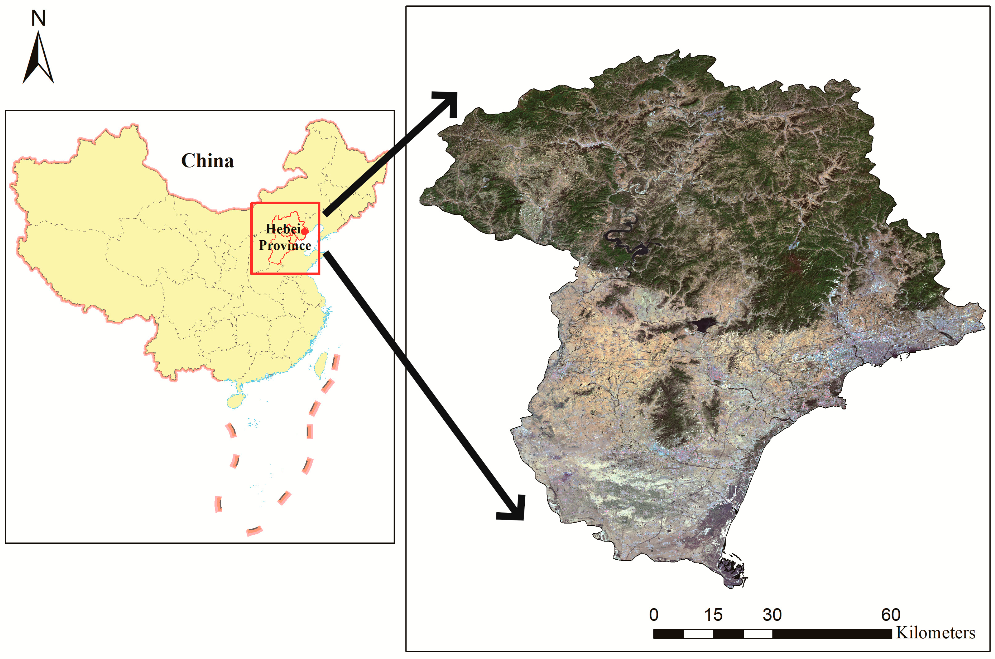
Qinhuangdao City was chosen as the case study site (Figure 1). It is located in the northeastern part of Hebei Province, north of Yanshan, south of Bohai, east of Huludao City in Liaoning Province, and west of Tangshan City in Hebei Province. The geographical coordinates range from 39°24′ to 40°37′N and from 118°33′ to 119°51′E, and the total area is approximately 7813 km2. Qinhuangdao has a generally warm temperate semi-humid continental monsoon climate. However, due to the influence of the adjacent Bohai Sea, the climate is milder, the summer is hot and rainy, the winter is dry and less rainy, and the average annual precipitation is approximately 652 mm. Qinhuangdao City is located in the eastern part of the Yanshan Mountains. The terrain is high in the north and low in the south; the northern part of the study is mountainous and mostly contains forest and grassland, and the southern part is a plains area, which is the main area of farmland and towns [23,24].
2.2. Data and Pre-Processing
The experiment used Landsat-8 satellite data. Landsat-8 is an Earth resource satellite launched by NASA that carries two sensors, OLI (Operational Land Imager) and TIRS (Thermal Infrared Sensor) [25]. This study mainly uses the multispectral band (B1-B7) of the Landsat-8 OLI data, and the satellite images acquisition times are 4 May 2015, 20 May 2015, and 13 May 2016.
Before using the convolutional neural network model to extract land cover information, it is necessary to perform the required pre-processing operations on the satellite imagery [26], including: (1) Radiation calibration and atmospheric correction. Using radiometric calibration, the DN values recorded by the sensor are converted into radiance values with actual physical meanings (i.e., apparent reflectance) [27]. ENVI’s FLAASH (Fast Line-of-sight Atmospheric Analysis of Hypercubes) atmospheric correction tool is then used to eliminate the effects of atmospheric scattering and absorption and obtain the surface reflectivity. (2) Image mosaic and cropping. Due to the large study area, the three scene images covering the study area are combined into a complete image covering Qinhuangdao City using inlaying operations and then cut according to the boundary of the study area.
In the study, based on the medium-high spatial resolution land cover mapping technical requirements and the actual conditions of the land cover in Qinhuangdao, the comparability of the results with other representative land cover and land use products at home and abroad must be considered. Therefore, the land surface types are divided into the following seven types: cultivated land, woodland, grassland, wetland, water body, building land and bare land. This classification is compatible with the first category of Globeland30 released by the national geographic information center.
3. Methodology
3.1. General Process
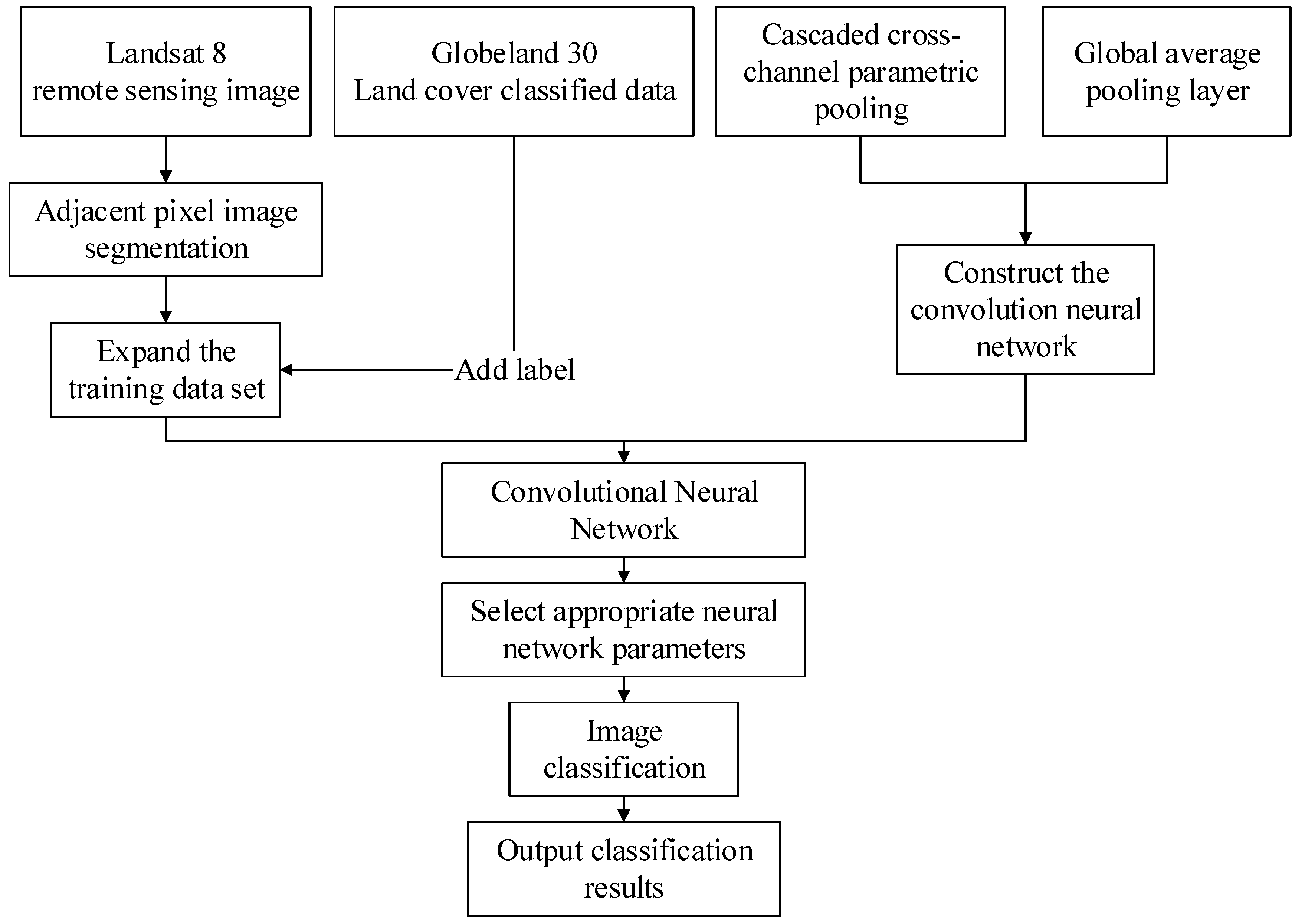
The DCNN-based medium-high-resolution remote sensing image land cover information extraction technology proposed in this paper includes the following four main steps: dataset construction, DCNN structure design, model training and parameter optimization, and image classification. The specific process is as follows (Figure 2):
Creating the training dataset. As a supervised classification method, the DCNN model requires a certain amount of learning material. This study designed a method for automatically arranging training samples, increasing the number of training samples, and obtaining accurate land cover information and corresponding spectral information from the training samples.
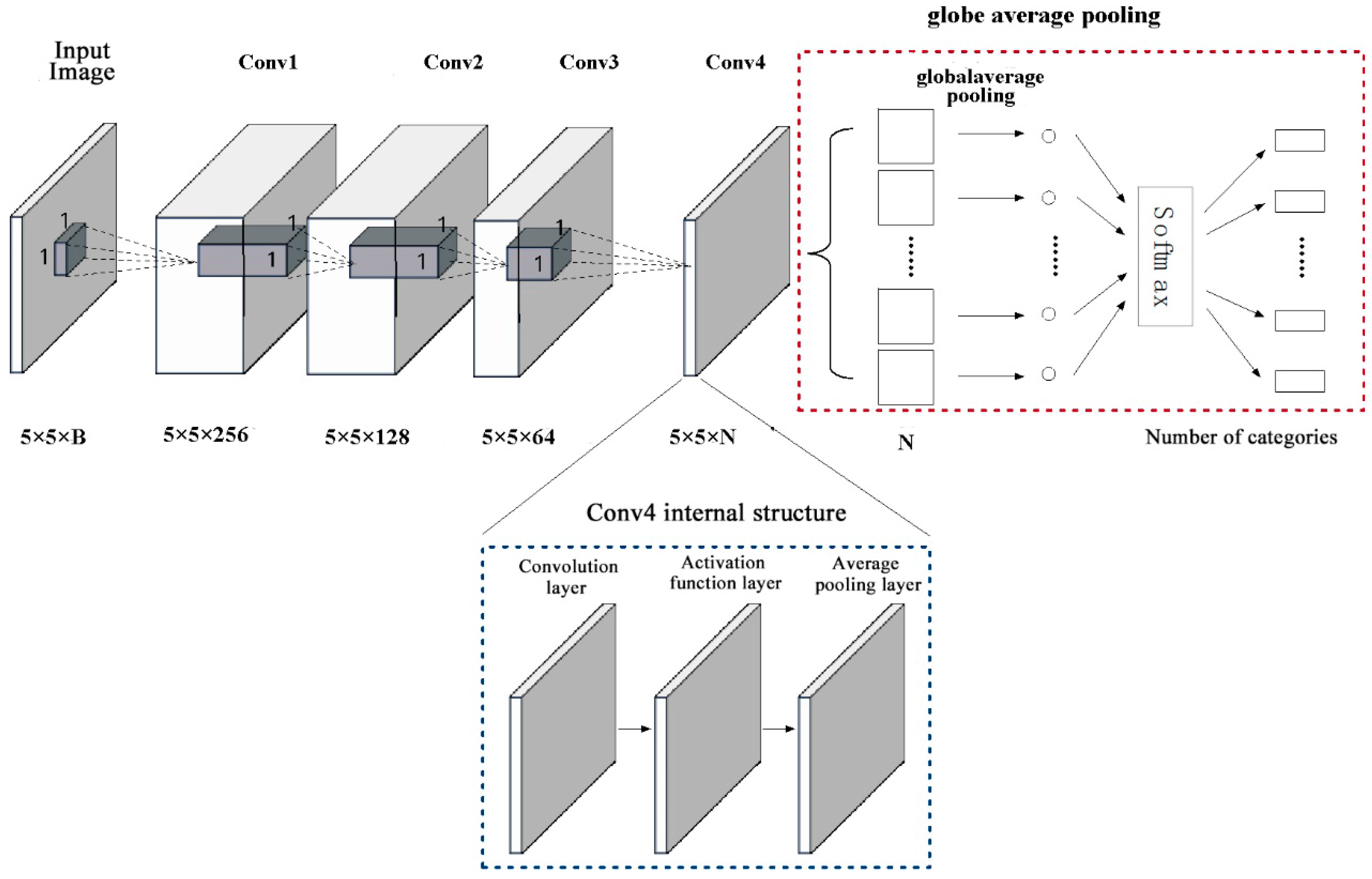
Building a deep convolutional neural network. Due to the fact that the existing DCNN model cannot adapt to multispectral satellite imagery and has poor generalization ability, this study designed cascaded cross-channel parametric pooling and a global average pooling layer, thus forming land cover suitable for medium-high-resolution remote sensing imagery.
Performing model training and parameter optimization. Taking the training dataset described above as input, the deep convolutional neural network is trained. Based on the loss value and accuracy curve obtained after the training, the training time length is comprehensively considered, and the relevant parameters of the final land cover classification are determined.
Land cover classification using satellite imagery. Applying the knowledge obtained from the deep neural network training described above and the results of the parameter optimization, the land cover information is extracted from the remote sensing image, and the land classification results of the study area are obtained.
3.2. Traditional Convolutional Neural Network
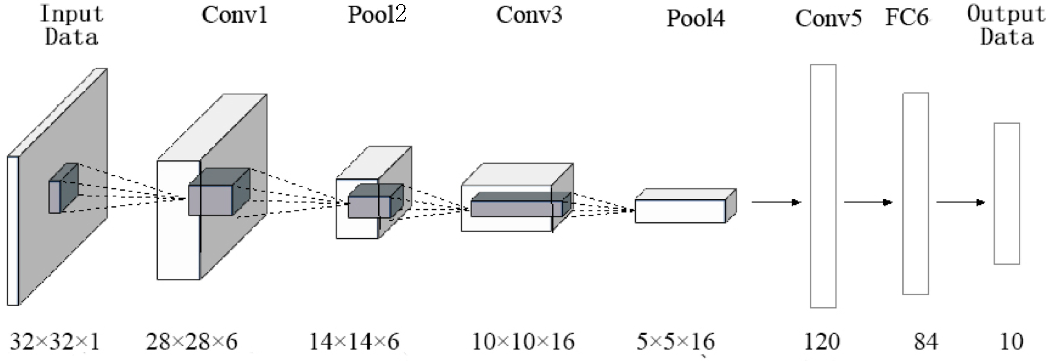
A convolutional neural network (CNN) is a multi-layer feed-forward neural network that is designed specifically to process large scale images or sensory data in the form of multiple arrays by considering local and global stationary properties [28,29]. In the neural network model, each neuron is a nonlinear regression model that is used to discriminate the relationship between the data to be classified and the classification results, and a large number of neurons combine to form a neural network [21]. Traditional convolutional neural network models (such as LeNet5) are mainly composed of a convolutional layer, a pooled layer and a fully linked layer [30] (Figure 3). In Figure 3, the Conv1, Conv3, and Conv5 layers are convolutional layers, the Pool2 and Pool4 layers are pooled layers, the FC6 layer is a full-link layer, and the last layer (7th layer) is the result output layer.
The traditional convolutional neural network model has a relatively simple structure and is deficient for application to remote sensing image classification research. The main problems are as follows: (1) the traditional LeNet5 model can only perform image classification for a single band and cannot extract information from multi-band remote sensing images and hyperspectral remote sensing images [31]; (2) the model uses a fully connected layer as a “classifier”, which is prone to parameter redundancy and overfitting, thereby reducing the generalization ability of the network [32]; and (3) the model can only output a single classification result for each image and cannot implement discriminant classification based on pixels or objects [33].
3.3. Cascaded Cross-Channel Parametric Pooling
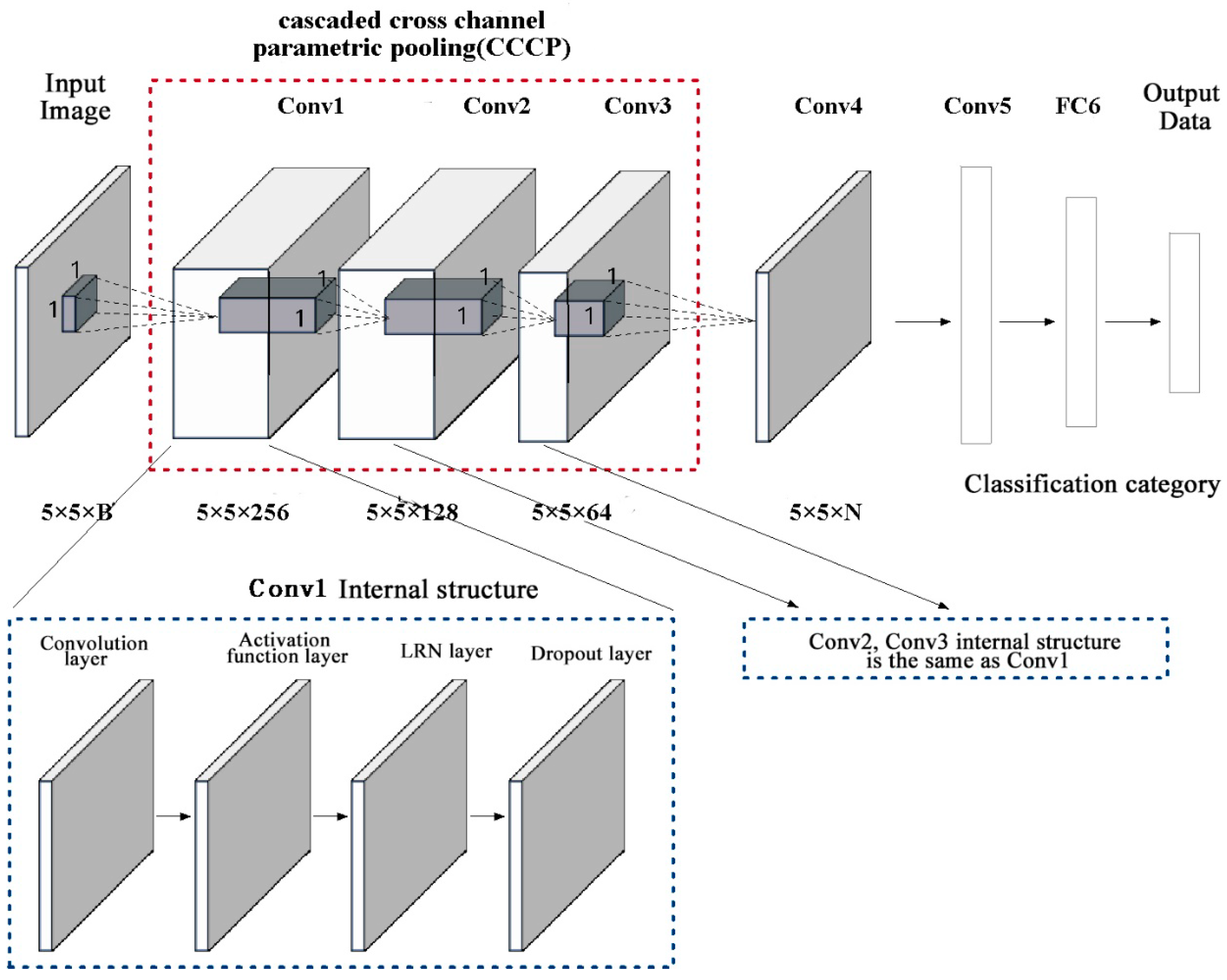
The classical convolutional neural network model can only be used for single bands or small numbers of bands (such as RGB three-band images). Due to the failure to make full use of the rich spectral band information in multispectral and hyperspectral satellite remote sensing images, the traditional convolutional neural network model has insufficient information utilization ability and low classification accuracy in satellite remote sensing land cover information extraction. In response to these problems, this study used the cascaded cross-channel parametric pooling (CCCP) method in the classical deep neural network model [34,35] (Figure 4). The CCCP layer is essentially a convolutional layer with a convolution kernel size of 1 × 1. The function of the convolution kernel is to perform linear combination calculations on the values at the same position in different bands to integrate the spectral information of different bands.
To strengthen the nonlinear characteristics of the network, this study connects a nonlinear activation function after each CCCP layer; this function can solve the linear indivisible problem for each convolution layer without losing the resolution of the feature image. After the nonlinear activation function layer, the local response normalization (LRN) layer is designed. The LRN layer can normalize the local input data to complete the "near suppression" operation and improve the classification accuracy of the network.
There are several advantages to introducing a CCCP layer. First, when multispectral or hyperspectral land cover information extraction is carried out, the CCCP layer can be used to adjust the feature map to achieve the dimension increase or decrease of the number of bands, thus achieving the compatibility of the DCNN method for multispectral remote sensing and hyperspectral remote sensing. Second, the flexible use of the 1 × 1 convolution kernel in the CCCP layer can realize the spectral information interaction and the integration of specific bands of remote sensing images, thereby improving the ability of the DCNN model to extract information about specific land cover types. For example, the CCCP method can be used to integrate the 5, 4, and 3 (NIR, red, and green) bands of the Landsat 8 OLI to better identify vegetation.
3.4. Global Average Pooling
Traditional convolutional neural networks usually use a fully connected layer as a “classifier” [36]. However, the fully connected layer is prone to parametric redundancy, which in turn causes overfitting and ultimately reduces the generalization ability of the neural network. To solve this problem, this paper introduces the dropout method in each CCCP layer [34] (Figure 4) and designs a global average pooling layer (GAP) after the activation function layer in the last convolution process [37,38] (Figure 5).
The function of the dropout in the CCCP layer is to randomly discard some neural network units from the network during each training session. Because each sub-network used for training is different, it is possible to prevent the neural network from overfitting the training data, thereby increasing the adaptability of the neural network algorithm to fresh samples and improving the generalization ability of the neural network [39].
The function of the global average pooling layer is to average the feature values of the respective pixels in each feature map, and the average value is taken as the probability value of each feature. After applying the global average pooling layer method, the number of feature maps output by the DCNN model is equal to the final number of land classification categories, and the information on the feature map characterizes the membership probability value of a certain land category, which can be further output to the softmax layer for final type discrimination. The introduction of the global average pooling layer allows the pixel-by-pixel and object-by-object classification of the DCNN model for a satellite remote sensing image.
The softmax layer performs the type discrimination as follows:
where Z is the input data, i is the number of categories of the classification, and is the probability distribution of the category to which the input data Z belongs.
3.5. Automatic Construction of the Training Dataset
After the introduction of the global average pooling layer, it is already technically possible to ensure the probability value of the land cover type for which the pixel-by-pixel discrimination is output. In addition, a complete set of pixel-based DCNN model training datasets is needed. Building a high-quality training dataset is a key step in the traditional neural network model training process. The construction of training datasets requires the selection and labeling of a large number of training samples, and the selection and labeling process is often time consuming and labor-intensive. For general life and production scene photos, manual labeling can be performed through network crowdsourcing, but this method is not appropriate for satellite remote sensing land cover information extraction work; due to the inaccessibility of land object objects and land cover and the professionalism of land use classification and discrimination, the manual marking method is not realistic. Therefore, this study proposes a method for automated deployment, expansion, and labeling of training points based on high-quality land cover products. The specific process as follows:
Using the stratified sampling method to randomly define training points within the study area; centered on these training points, the satellite image is cut into fragments of 5 × 5 pixels, and each image fragment becomes a training sample.
To improve the diversity of the training dataset and not actually increase the number of training samples, the image fragments are rotated (by 0°, 90°, 180°, 270°) and mirrored (up and down mirror, left and right mirror). The method is transformed, thereby expanding the number of samples in the training dataset to 8 times the number of original training points.
Relying on the globally recognized Globeland30 2010 product, which has the highest spatial resolution and highest overall accuracy (spatial resolution of 30 m and overall accuracy of 80% or more), based on the principles of geospatial position, the property attributes are extracted pixel by pixel from the Glbeland30 product, and each fragment image is identified.
Using this method, a training dataset at the pixel scale can be constructed. Because the Globeland30 2010 land cover product information is automatically extracted at the corresponding location, there is no need to visually interpret or otherwise label the training samples. This greatly reduces the labor and time costs and ensures the quality of the training dataset.
3.6. Training Samples and Training Process
First, the model training sample selection and the automatic extraction of the Globeland30 land information were carried out in the study area using stratified random deployment training samples. Generally, the training sample volume accounts for 1% of the total number of pixels in each class (such as cultivated land and forest). For some types of land (such as wetlands and bare land), where the area is small or the distribution is particularly sporadic, which results in a small number of randomly deployed samples, the number of samples is increased to ensure that the number of training samples for each land cover type is at least approximately 4000. A total of 112,226 training samples were selected in the study area, which represented approximately 1.3% of all of the pixels in the study area (Table 1).
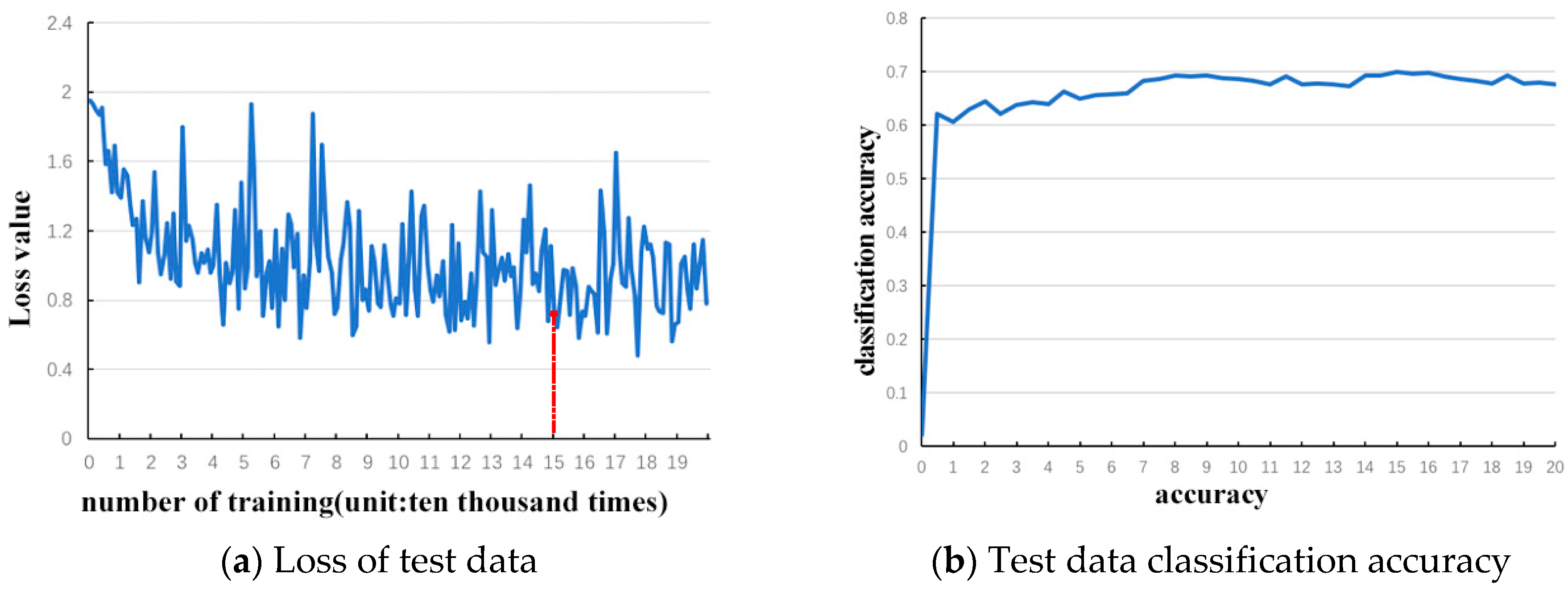
Based on automatic selection and information extraction of the training samples, deep training of the deep neural networks was carried out using these training datasets as inputs. The loss value of the DCNN model in the training process was recorded (i.e., the negative value of the logarithm of the probability that the pixel to be classified is divided into real categories; for example, if the probability that the pixel to be classified is divided into real categories is 0.6, the loss value is -log0.6), and the relationship between the accuracy of the overall classification results and the number of trainings was determined (Figure 6). The lower the loss value, the higher the accuracy of the classification result.
Figure 6 shows that as the number of trainings increases, the loss value decreases rapidly and then continues to maintain the wave dynamic potential, and the classification accuracy will increase rapidly with increasing number of trainings and then become stable. Based on this variation and considering the accuracy of the results obtained by the DCNN and the running time of the model, the authors selected the resulting parameters of the model that was trained 150,000 times for the final remote sensing image land classification.
4. Analysis of Results
4.1. Land Maps and Visual Contrast
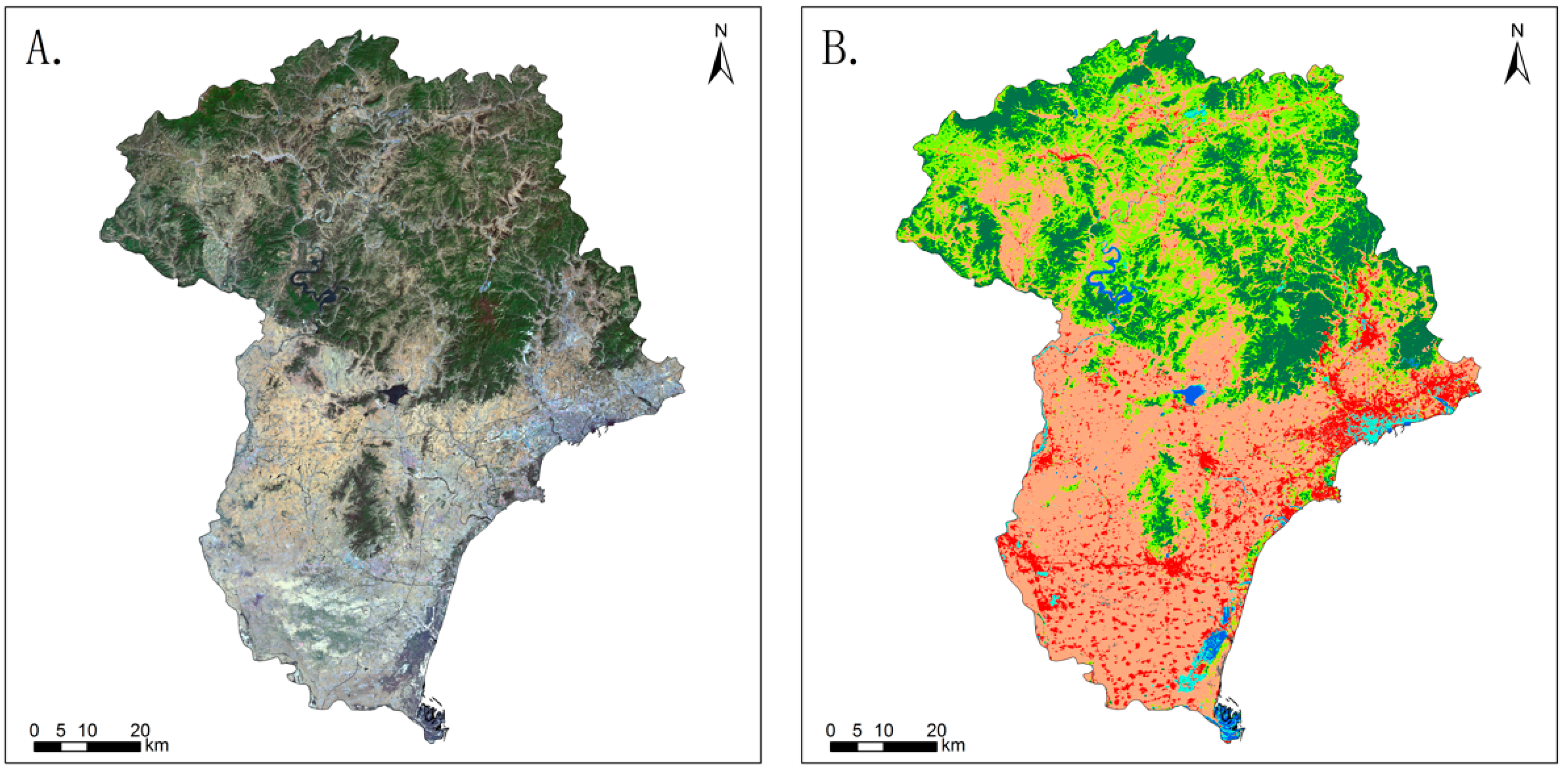
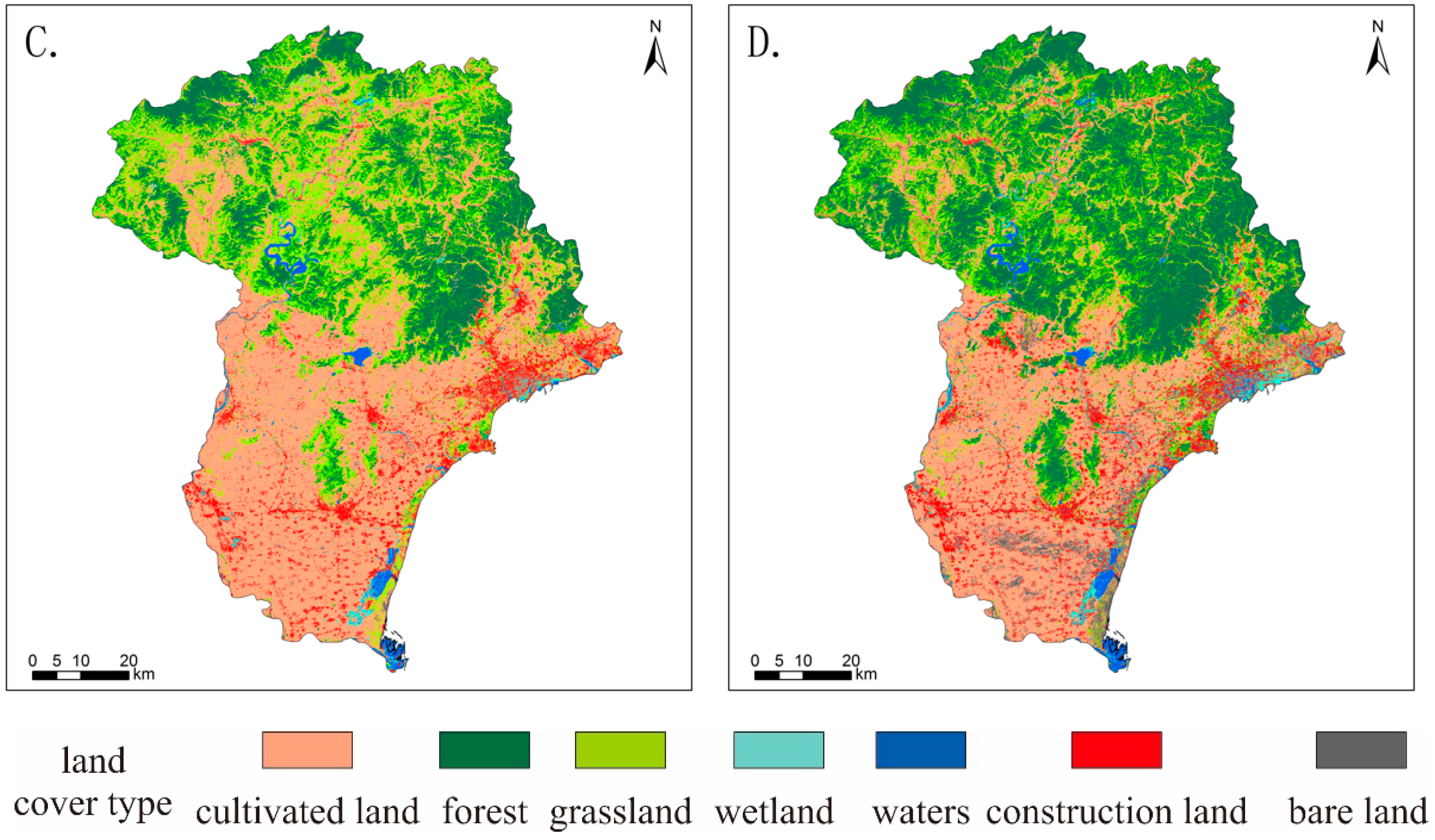
Applying the DCNN model framework and the training optimization model parameter scheme described above, the 7-band data of Landsat 8 OLI B1-B7 is input (Figure 7A), and the spatial distribution of the land cover in the Qinhuangdao area can be obtained (Figure 7B). To compare and evaluate the DCNN results, this study also used a support vector machine (SVM) (Figure 7C) and maximum likelihood classification (MLC) (Figure 7D) to compare the classification results. The SVM method uses the method provided by ENVI 5.2, the inner product kernel is the radial basis function, the gamma in the kernel function is 0.143, the penalty parameter is 100, and the classification probability threshold is 0. The MLC method also uses the ENVI 5.2 tool module, in which the likelihood threshold is set to none, and the scale factor is the maximum reflectance data.
Figure 7 shows that the results obtained by the three methods can accurately reflect the basic spatial distribution of land cover in Qinhuangdao. The northern region of Qinhuangdao is a key ecological zone, and forest and grassland are the main types of land cover. In addition, the area contains large reservoirs, rivers and other water bodies, which play important ecological functions, such as wind and sand fixation and water conservation. The southern region is a plains landform and is part of the Haihe-Liaohe alluvial plain. It is a core area of agricultural production in Qinhuangdao and is dominated by cultivated land. In the eastern coastal area, there is a dense distribution of construction land, a large number of forests, and grasslands and water bodies are scattered around the cultivated land and construction land. In addition, there are large areas of forest in the central and eastern regions. In the central part of Qinhuangdao, there are large areas of water, such as the Yanghe Reservoir and the Taolinkou Reservoir. A large area of estuaries and coastal wetlands is located in the Luanhekou area in the southeastern region.
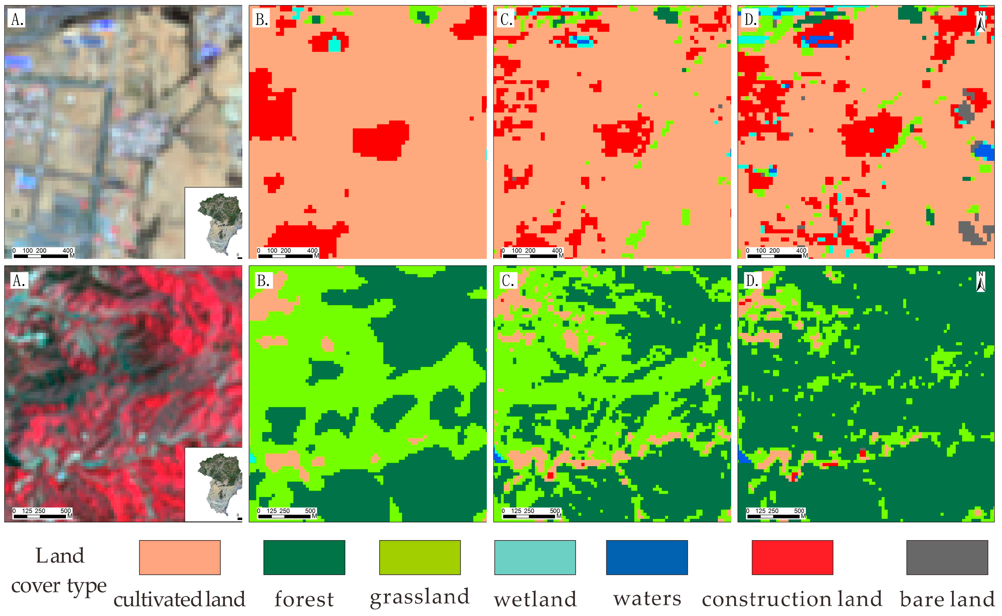
A comparison of the results of the three methods (Figure 8) shows that in the central and southern parts of Qinhuangdao, the SVM and MLC methods show more compact areas of construction land, and the distribution is more scattered. The area obtained by the DCNN method is slightly larger and is more concentrated (Figure 8, first row). This is because in the DCNN land classification process, the type attribute of the cell to be classified depends not only on the spectral characteristics of the cell itself but also on the types of the surrounding cells. Because the DCNN model in this study uses a 5 × 5 pixel training sample library for classification, it will expand the identification boundary of the scattered rural settlement land (or other scattered land cover type). The resulting benefit is that DCNN has a significant inhibitory effect on the “salt and pepper” phenomenon observed in traditional automated satellite imagery classification methods.
In addition, in the northern part of Qinhuangdao, the three classification methods can generally identify woodland and grassland well, but there are significant differences between the details of the classification results of the two land types (Figure 8, second row). The DCNN and SVM classification methods can accurately identify forest on shaded slopes and grassland on the sunny slopes in the mountains. However, using the MLC method, the land on shaded slopes and sunny slopes in the mountains is mostly identified as forest. The DCNN method is clearly superior to the MLC method in discriminating forest and grassland types, which have spectral characteristics that are easily confused.
4.2. Accuracy Assessment
We randomly selected 820 verification points in the study area, and based on a high-resolution satellite remote sensing image provided by Google Earth, a visual interpretation was performed, and the confusion matrix method was used to carry out a quantitative evaluation of the accuracy of the land classification results (Table 2).
The results show that the overall accuracies of the DCNN, SVM and MLC classifications are between 67.5% and 82.0%, and the kappa coefficients are between 0.58 and 0.76. The proposed DCNN classification provides the best results; the overall accuracy is 82.0%, and the kappa coefficient is 0.76. The SVM classification gives the second-best results with an overall accuracy of the land classification of 76.8% and a kappa coefficient of 0.69. The MLC method gives the worst classification; the overall accuracy is only 67.6%, and the kappa coefficient is only 0.58.
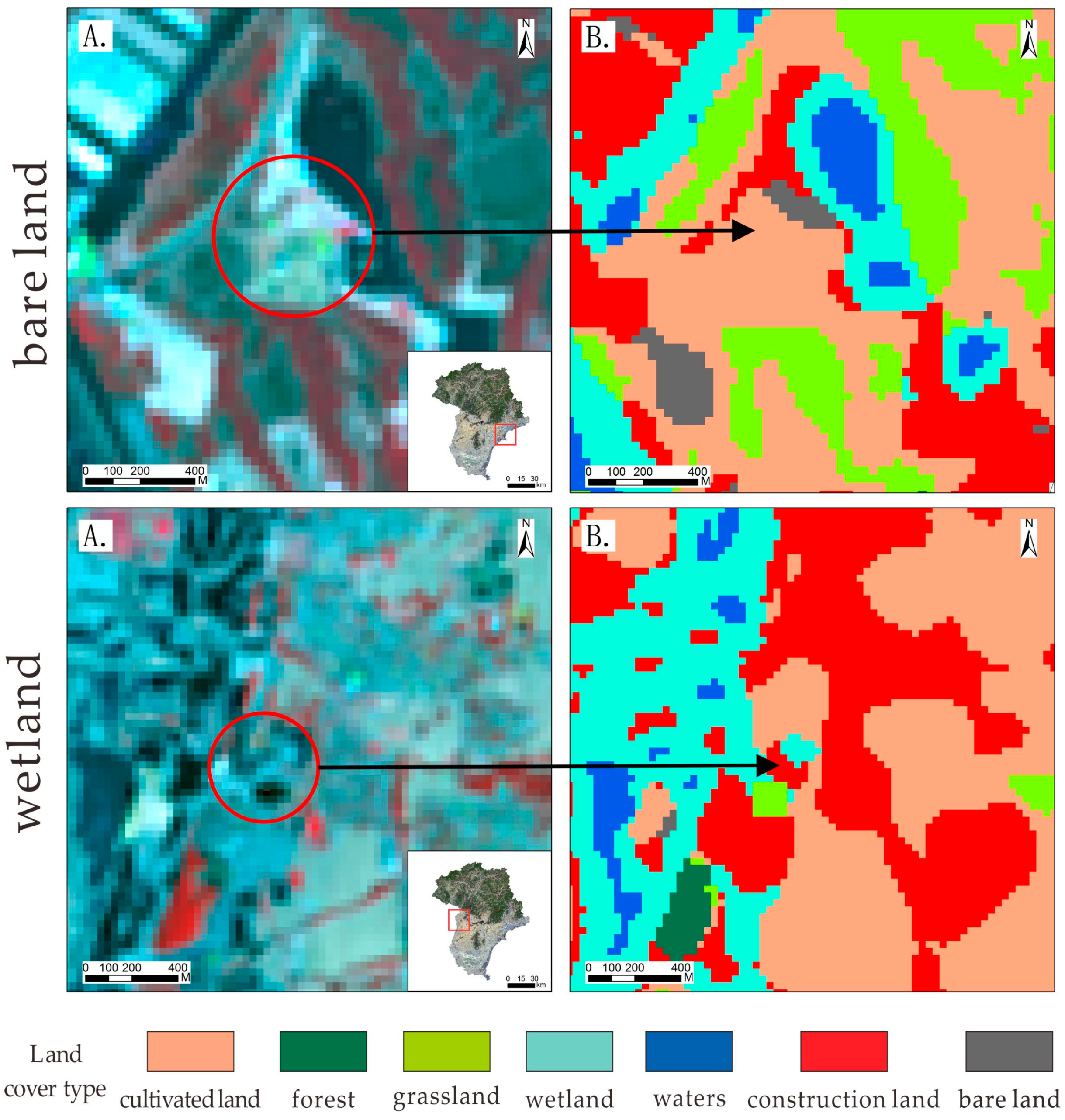
For the DCNN results (Table 3), bare land has the lowest producer’s accuracy (only 36.84%). Bare land is easily misclassified as cultivated land and construction land (42.1% and 21.0% of all pixels of these types, respectively) (Figure 8). This occurs for several reasons. First, the Qinhuangdao area contains a small amount of bare land, and only 4489 bare ground training samples were randomly obtained, which is the fewest of any category. Second, the number of randomly verified bare land verification points is particularly small (only 19), so the calculated error is easily exaggerated. Third, bare land, cultivated land, abandoned farmland, and urban and rural construction land have similar physical properties, and their differences are mainly reflected in the different land use patterns. The similarity in the surface physical characteristics can easily lead to misjudgments between bare land, cultivated land and construction land.
The producer’s accuracy of construction land is also low (58.11%). Some construction land is particularly vulnerable to misidentification as cultivated land (31.1% of all pixels of this type) because in the vast rural areas of the central and southern parts of the study area, a large amount of rural residential land is scattered throughout the cultivated land (Figure 8). In the DCNN classification, the type of cell to be classified depends not only on the spectral characteristics of the cell itself but also on the types of surrounding cells. When the pixel to be classified is construction land and the surrounding pixels are cultivated land, the pixel can easily be classified as cultivated land by the DCNN model. The second reason is similar to the reason that the bare land is misclassified. The final goal is to form a land category for urban and rural residential and living production land. This land usually goes through a process from arable land to bare land and finally to buildings and impervious surfaces. Changes in land use patterns are difficult to distinguish from land cover types.
The wetlands user accuracy (64.5%) is also relatively low. Wetlands are easily misclassified as construction land (22.6% of all pixels of this type) (Figure 9) because the wetlands are mostly distributed in the areas surrounding lakes and rivers, the terrain along the rivers is flat, and there are many rural construction sites in the areas near water sources. During the classification process, because the boundaries between the wetlands and the construction land near the river are not clear, the wetlands at the edge of the city are easily classified as construction land, resulting in a misclassification between the wetlands and the construction land.
5. Discussion
5.1. Cause of the Difference in Accuracy
In general, different classification methods have different classification accuracies due to many complex factors, such as the principles of the classification, the object to be classified, the size of training sample library, and the classification threshold settings. Comparing the classification accuracies of different methods and analyzing the causes of the differences in precision are interesting topics in remote sensing application research. It is generally believed that in land cover mapping, there is no significant difference in accuracy between the SVM classification method and the MLC classification method [40,41]. The SVM method is reliable with a small number of training samples, and the MLC method performs the classification more quickly [42,43].
In our case study, the DCNN method performed better than the other two methods. We speculate that this may be related to the properties of the peripheral pixels (5*5) around the target pixel and their relationship with each other when the DCNN is trained, whereas the SVM and MLC methods are simply pixel-based classification methods. The MLC method considers less information than the DCNN does, which may be the reason for its lowest classification accuracy. However, to prove this hypothesis, it is necessary to conduct a comparative study on the relevant classifier parameter settings in the MLC and SVM classification processes and the adjacent pixel size setting in the DCNN classification process.
5.2. Comparison with Other CNN Models
The application of convolutional neural network methods in land cover mapping is progressing very rapidly [44,45]. Xu et al. [46] developed a three-dimensional convolutional neural network method for land cover classification using intensity information from LiDAR (Light Detection And Ranging) and multi-temporal Landsat images. The method is believed to be able to capture a wide range of complex features of various land cover types; however, it requires a large training sample library, and Xu did not present an automated construction scheme for such training datasets. Atharva Sharma et al. [47] proposed a new patch-based recurrent neural network (PB-RNN) for land cover classification based on the spatial and sequential interdependence between adjacent pixels. It has a high classification accuracy for multi-temporal and multispectral remote sensing images but is not implemented for single-scene images.
Compared with these CNN land mapping frameworks, our new framework and processes can automatically build a large training sample library and avoids the “salt and pepper” phenomenon after pixel classification using cascaded cross-channel parametric pooling and an average pooling layer. This CNN method also has a higher classification accuracy than traditional methods and is suitable for single-time and multi-temporal remote sensing images. The shortcoming of our CNN model framework is that it requires more computer resources than traditional classification methods and all other CNN models. In addition, our method is currently only applicable to pixel-level image classification, which means that it is only suitable for medium-high-resolution imagery (i.e., Landsat-like series) and not for high-resolution satellite imagery (e.g., SPOT, Sentinel, GF1/2).
6. Conclusions
Based on the classical DCNN model, this paper introduced a cascaded cross-channel parametric pooling and the global average pooling method. A new technical framework for satellite remote sensing land cover mapping based on a deep convolutional neural network was proposed, and a practical image classification and result analysis was performed in Qinhuangdao City, Hebei Province. The results of this research show that:
The ordinary DCNN model method is difficult to apply to multispectral and hyperspectral satellite remote sensing land information extraction. Cascaded cross-channel parametric pooling and the global average pooling method can effectively solve this problem and enhance the generalization ability of the DCNN model, which helps to achieve pixel-by-pixel classification of satellite images. Based on the stratified random sampling strategy and the high-precision land use and land cover product, the land type information extraction method addresses the problem that the traditional DCNN methods are time-consuming and labor-intensive in constructing a high-quality training sample library.
The proposed DCNN model had the best accuracy in the comparison of land cover information extraction in Qinhuangdao City. The overall accuracy of the land classification results of the proposed DCNN model is 82.0%, and the kappa coefficient is 0.76. Compared with the traditional support vector machine (SVM) method and the maximum likelihood classification (MLC) method, the overall accuracy of the results obtained by the DCNN model method is 5% and 14% higher, respectively, and the kappa coefficient is 0.07 and 0.18 higher, respectively.
This study also revealed several problems in the field of land cover mapping supported by deep neural network methods. Although the CNN method requires higher performance hardware, such as the CPU and GPU, it runs more slowly on a traditional computer. In the future, a cloud environment, such as GEE (Google Earth Engine), AWS (Amazon Web Services), and Aliyun (Alibaba Cloud), combined with a large-scale GPU, should be considered to improve the calculation speed and reduce the regional land cover mapping time. However, the research presented in this paper is at the pixel scale, and it is mainly suitable for medium- and high-resolution satellite imagery. For high-resolution satellite remote sensing images (especially images below 5 m, such as SPOT satellite image and GF1/2 satellite image), multi-scale segmentation and object-oriented methods can be further combined in the future to improve the accuracy of regional high-resolution satellite remote sensing land cover information extraction.
Although the land cover results interpreted by the CNN method are more accurate than those obtained by traditional methods, the CNN method usually requires more computer resources and requires a CPU and GPU with higher performances. Therefore, a more appropriate scenario in the future is to deploy the CNN framework in cloud computing environments, such as GEE (Google Earth Engine), AWS (Amazon Web Services) and Aliyun (Alibaba Cloud), as well as large-scale GPU clusters. Moreover, the proposed DCNN land mapping framework is suitable for moderate- to high-resolution satellite imagery land cover mapping and annual land cover updates at large scales. However, higher-resolution land use mapping requires additional detailed studies.
Author Contributions
Y.H. designed and supervised the research. Q.Z. performed the experiments and preliminarily analyzed the results. All of the authors drafted and revised the paper.
Funding
This work was supported by the National Key Research and Development Program of China under Grant No. 2016YFC0503702; the Strategic Priority Research Program of CAS under Grant No. XDA19040301; and the Key Project of High-Resolution Earth Observation of China under Grant No. 00-Y30B14-9001-14/16.
Conflicts of Interest
The authors declare no conflicts of interest.
References
- Weng, Q.; Lu, D. A sub-pixel analysis of urbanization effect on land surface temperature and its interplay with impervious surface and vegetation coverage in Indianapolis, united states. Int. J. Appl. Earth Obs. 2008, 10, 68–83. [Google Scholar] [CrossRef]
- Cadenasso, M.L.; Pickett, S.T.; Schwarz, K. Spatial heterogeneity in urban ecosystems: Reconceptualizing land cover and a framework for classification. Front. Ecol. Environ. 2007, 5, 80–88. [Google Scholar] [CrossRef]
- Patino, J.E.; Duque, J.C. A review of regional science applications of satellite remote sensing in urban settings. Comput. Environ. Urban Syst. 2013, 37, 1–17. [Google Scholar] [CrossRef]
- Liu, J.; Kuang, W.; Zhang, Z.; Xu, X.; Qin, Y.; Ning, J.; Zhou, W.; Zhang, S.; Li, R.; Yan, C. Spatiotemporal characteristics, patterns, and causes of land-use changes in China since the late 1980s. J. Geogr. Sci. 2014, 24, 195–210. [Google Scholar] [CrossRef]
- Quesada, B.; Arneth, A.; Noblet-Ducoudré, N. Atmospheric, radiative, and hydrologic effects of future land use and land cover changes: A global and multimodel climate picture. J. Geophys. Res. Atmos. 2017, 122, 5113–5131. [Google Scholar] [CrossRef]
- Cihlar, J. Land cover mapping of large areas from satellites: Status and research priorities. Int. J. Remote Sens. 2000, 21, 1093–1114. [Google Scholar] [CrossRef] [Green Version]
- Chen, J.; Chen, J.; Liao, A.; Cao, X.; Chen, L.; Chen, X.; He, C.; Han, G.; Peng, S.; Lu, M. Global land cover mapping at 30 m resolution: A pok-based operational approach. ISPRS J. Photogramm. Remote Sens. 2015, 103, 7–27. [Google Scholar] [CrossRef]
- Hu, Y.; Nacun, B. An analysis of land-use change and grassland degradation from a policy perspective in inner mongolia, China, 1990–2015. Sustainability 2018, 10, 4048. [Google Scholar] [CrossRef]
- Claas, B.; Yunfeng, N.; Tobia, H. Land-use change and land degradation on the mongolian plateau from 1975 to 2015—A case study from Xilingol, China. Land Degrad. Dev. 2018, 29, 1595–1606. [Google Scholar]
- Pohl, C.; Van Genderen, J.L. Review article multisensor image fusion in remote sensing: Concepts, methods and applications. Int. J. Remote Sens. 1998, 19, 823–854. [Google Scholar] [CrossRef]
- Petit, C.; Lambin, E. Integration of multi-source remote sensing data for land cover change detection. Int. J. Geogr. Inf. Sci. 2001, 15, 785–803. [Google Scholar] [CrossRef]
- Yang, W.; Dai, D.; Triggs, B.; Xia, G. Sar-based terrain classification using weakly supervised hierarchical markov aspect models. IEEE Trans. Image Process. 2012, 21, 4232. [Google Scholar] [CrossRef] [PubMed]
- Attarchi, S.; Gloaguen, R. Classifying complex mountainous forests with l-band sar and landsat data integration: A comparison among different machine learning methods in the Hyrcanian forest. Remote Sens. 2014, 6, 3624–3647. [Google Scholar] [CrossRef]
- Gómez, C.; White, J.C.; Wulder, M.A. Optical remotely sensed time series data for land cover classification: A review. ISPRS J. Photogramm. Remote Sens. 2016, 116, 55–72. [Google Scholar] [CrossRef]
- Hu, Y.; Dong, Y.; Batunacun. An automatic approach for land-change detection and land updates based on integrated NDVI timing analysis and the CVAPS method with GEE support. ISPRS J. Photogramm. Remote Sens. 2018, 146, 347–359. [Google Scholar] [CrossRef]
- Noszczyk, T. A review of approaches to land use changes modeling. Hum. Ecol. Risk Assess. 2018, 28, 1–29. [Google Scholar] [CrossRef]
- Liu, T.; Abd-Elrahman, A.; Morton, J.; Wilhelm, V.L. Comparing fully convolutional networks, random forest, support vector machine, and patch-based deep convolutional neural networks for object-based wetland mapping using images from small unmanned aircraft system. GISci. Remote Sens. 2018, 55, 243–264. [Google Scholar] [CrossRef]
- Cheng, G.; Yang, C.; Yao, X.; Guo, L.; Han, J. When deep learning meets metric learning: Remote sensing image scene classification via learning discriminative CNNs. IEEE Trans. Geosci. Remote Sens. 2018, 56, 2811–2821. [Google Scholar] [CrossRef]
- Nogueira, K.; Penatti, O.A.; dos Santos, J.A. Towards better exploiting convolutional neural networks for remote sensing scene classification. Pattern Recognit. 2017, 61, 539–556. [Google Scholar] [CrossRef] [Green Version]
- Basaeed, E.; Bhaskar, H.; Al-Mualla, M. Supervised remote sensing image segmentation using boosted convolutional neural networks. Knowl. Based Syst. 2016, 99, 19–27. [Google Scholar] [CrossRef]
- Yu, S.; Jia, S.; Xu, C. Convolutional neural networks for hyperspectral image classification. Neurocomputing 2017, 219, 88–98. [Google Scholar] [CrossRef]
- Huang, B.; Zhao, B.; Song, Y. Urban land-use mapping using a deep convolutional neural network with high spatial resolution multispectral remote sensing imagery. Remote Sens. Environ. 2018, 214, 73–86. [Google Scholar] [CrossRef]
- Zhang, S.; Zhu, Q.; Gu, J. Responses of regional ecological service value to land use change—A case study of Qinhuangdao city. J. Shanxi Normal Univ. 2010, 1, 26. [Google Scholar]
- Zhang, J. Study on the ecological regionalization in qinhuangdao city based on gis graticule method. J. Anhui Agric. Sci. 2008, 35, 9088. [Google Scholar]
- Roy, D.P.; Wulder, M.; Loveland, T.R.; Woodcock, C.; Allen, R.; Anderson, M.; Helder, D.; Irons, J.; Johnson, D.; Kennedy, R. Landsat-8: Science and product vision for terrestrial global change research. Remote Sens. Environ. 2014, 145, 154–172. [Google Scholar] [CrossRef]
- Hansen, M.C.; Loveland, T.R. A review of large area monitoring of land cover change using landsat data. Remote Sens. Environ. 2012, 122, 66–74. [Google Scholar] [CrossRef]
- Czapla-Myers, J.; McCorkel, J.; Anderson, N.; Thome, K.; Biggar, S.; Helder, D.; Aaron, D.; Leigh, L.; Mishra, N. The ground-based absolute radiometric calibration of landsat 8 oli. Remote Sens. 2015, 7, 600–626. [Google Scholar] [CrossRef]
- LeCun, Y.; Bengio, Y.; Hinton, G. Deep learning. Nature 2015, 521, 436. [Google Scholar] [CrossRef]
- Zhang, C.; Sargent, I.; Pan, X.; Li, H.; Gardiner, A.; Hare, J.; Atkinson, P.M. An object-based convolutional neural network (OCNN) for urban land use classification. Remote Sens. Environ. 2018, 216, 57–70. [Google Scholar] [CrossRef]
- LeCun, Y.; Bottou, L.; Bengio, Y.; Haffner, P. Gradient-based learning applied to document recognition. Proc. IEEE 1998, 86, 2278–2324. [Google Scholar] [CrossRef] [Green Version]
- Zhou, H.; Wang, Y.; Lei, X.; Liu, Y. A Method of Improved CNN Traffic Classification. In Proceedings of the 13th International Conference on Computational Intelligence and Security (CIS), Hong Kong, China, 15–18 December 2017; pp. 177–181. [Google Scholar]
- Krenker, A.; Bešter, J.; Kos, A. Introduction to the Artificial Neural Networks. In Artificial Neural Networks: Methodological Advances and Biomedical Applications; Intech Open: London, UK, 2011; pp. 1–18. [Google Scholar]
- Nguyen, A.; Yosinski, J.; Clune, J. Deep Neural Networks are Easily Fooled: High Confidence Predictions for Unrecognizable Images; IEEE: Piscataway, NJ, USA, 2015; pp. 427–436. [Google Scholar]
- Lin, M.; Chen, Q.; Yan, S. Network in network. arXiv, 2013; arXiv:1312.4400. [Google Scholar]
- Valada, A.; Spinello, L.; Burgard, W. Deep Feature Learning for Acoustics-Based Terrain Classification; Springer: Berlin, Germany, 2018; pp. 21–37. [Google Scholar]
- Krizhevsky, A.; Sutskever, I.; Hinton, G.E. Imagenet Classification with Deep Convolutional Neural Networks. Adv. Neural Inf. Process. Syst. 2012, 20, 1097–1105. [Google Scholar] [CrossRef]
- Hinton, G.E.; Srivastava, N.; Krizhevsky, A.; Sutskever, I.; Salakhutdinov, R.R. Improving neural networks by preventing co-adaptation of feature detectors. arXiv, 2012; arXiv:1207.0580. [Google Scholar]
- Zhou, B.; Khosla, A.; Lapedriza, A.; Oliva, A.; Torralba, A. Learning Deep Features for Discriminative Localization; IEEE: Piscataway, NJ, USA, 2016; pp. 2921–2929. [Google Scholar]
- Srivastava, N. Improving neural networks with dropout. Univ. Toronto 2013, 182, 566. [Google Scholar]
- Erbek, F.S.; Özkan, C.; Taberner, M. Comparison of maximum likelihood classification method with supervised artificial neural network algorithms for land use activities. Int. J. Remote Sens. 2004, 25, 1733–1748. [Google Scholar] [CrossRef]
- Otukei, J.R.; Blaschke, T. Land cover change assessment using decision trees, support vector machines and maximum likelihood classification algorithms. Int. J. Appl. Earth Obs. Geoinf. 2010, 12, S27–S31. [Google Scholar] [CrossRef]
- He, J.; Harris, J.R.; Sawada, M.; Behnia, P. A comparison of classification algorithms using landsat-7 and landsat-8 data for mapping lithology in canada’s arctic. Int. J. Remote Sens. 2015, 36, 2252–2276. [Google Scholar] [CrossRef]
- Srivastava, P.K.; Han, D.W.; Rico-Ramirez, M.A.; Bray, M.; Islam, T. Selection of classification techniques for land use/land cover change investigation. Adv. Space Res. 2012, 50, 1250–1265. [Google Scholar] [CrossRef]
- Paoletti, M.; Haut, J.; Plaza, J.; Plaza, A. A new deep convolutional neural network for fast hyperspectral image classification. ISPRS J. Photogramm. Remote Sens. 2018, 145, 120–147. [Google Scholar] [CrossRef]
- Marcos, D.; Volpi, M.; Kellenberger, B.; Tuia, D. Land cover mapping at very high resolution with rotation equivariant cnns: Towards small yet accurate models. ISPRS J. Photogramm. Remote Sens. 2018, 145, 96–107. [Google Scholar] [CrossRef]
- Xu, Z.; Guan, K.; Casler, N.; Peng, B.; Wang, S. A 3d convolutional neural network method for land cover classification using lidar and multi-temporal landsat imagery. ISPRS J. Photogramm. Remote Sens. 2018, 144, 423–434. [Google Scholar] [CrossRef]
- Sharma, A.; Liu, X.; Yang, X. Land cover classification from multi-temporal, multi-spectral remotely sensed imagery using patch-based recurrent neural networks. Neural Netw. 2018, 105, 346–355. [Google Scholar] [CrossRef] [PubMed] [Green Version]
Figure 1.
Study area and image data: Qinhuangdao City Landsat8 (RGB: Bands 4, 3, 2).

Figure 2.
Flowchart of the land classification process using the deep convolutional neural network (DCNN) model.
Figure 2.
Flowchart of the land classification process using the deep convolutional neural network (DCNN) model.

Figure 3.
Framework of a typical convolutional neural network (CNN) model (LeNet5) (modified from reference [22]).
Figure 3.
Framework of a typical convolutional neural network (CNN) model (LeNet5) (modified from reference [22]).

Figure 4.
A convolutional neural network model with the the cascaded cross-channel parametric pooling (CCCP) layer (modified from reference [22]).
Figure 4.
A convolutional neural network model with the the cascaded cross-channel parametric pooling (CCCP) layer (modified from reference [22]).

Figure 5.
A convolutional neural network model with a global average pooling layer (modified from reference [22]).
Figure 5.
A convolutional neural network model with a global average pooling layer (modified from reference [22]).

Figure 6.
Trends of the CNN loss value and the accuracy of the results with increasing training time. (With increasing training time, the loss first decreases and then tends to be gentle, and the accuracy first increases and then tends to be gentle.)
Figure 6.
Trends of the CNN loss value and the accuracy of the results with increasing training time. (With increasing training time, the loss first decreases and then tends to be gentle, and the accuracy first increases and then tends to be gentle.)

Figure 7.
Comparisons between three true color classification methods based on pixels (A: Landsat 8 Operational Land Imager (OLI) (RGB: Bands 5, 4, 3), B: DCNN, C: support vector machine (SVM), and D: maximum likelihood classification (MLC)).
Figure 7.
Comparisons between three true color classification methods based on pixels (A: Landsat 8 Operational Land Imager (OLI) (RGB: Bands 5, 4, 3), B: DCNN, C: support vector machine (SVM), and D: maximum likelihood classification (MLC)).


Figure 8.
Comparison of three methods used for the detailed identification of artificial land in the south and forest land in the north (A: Landsat 8 OLI (RGB: Bands 5, 4, 3), B: DCNN, C: SVM, and D: MLC).
Figure 8.
Comparison of three methods used for the detailed identification of artificial land in the south and forest land in the north (A: Landsat 8 OLI (RGB: Bands 5, 4, 3), B: DCNN, C: SVM, and D: MLC).

Figure 9.
Detailed maps of bare land and wet land identification (A: Landsat 8 OLI (RGB: Bands 5, 4, 3); B: DCNN).
Figure 9.
Detailed maps of bare land and wet land identification (A: Landsat 8 OLI (RGB: Bands 5, 4, 3); B: DCNN).


Table 1.
Numbers of samples of different land cover types in Qinhuangdao.
| Number | Type of Land Cover | Total Number of Samples | Number of Training Samples | Percent |
|---|---|---|---|---|
| 1 | cultivated land | 3,714,833 | 37,252 | 1% |
| 2 | forest | 1,731,481 | 17,213 | 1% |
| 3 | grassland | 2,360,062 | 23,486 | 1% |
| 4 | wetland | 12,822 | 8117 | 63.6% |
| 5 | water | 88,280 | 8318 | 9.4% |
| 6 | construction land | 674,425 | 13,351 | 2.0% |
| 7 | bare land | 7108 | 4489 | 63% |
| total | 8,616,011 | 112,226 | 1.3% |
Table 2.
Comparison of the accuracies of the results of the DCNN, SVM and MLC methods.
| Method | DCNN | SVM | MLC |
|---|---|---|---|
| Overall accuracy (%) | 82.0 | 76.8 | 67.6 |
| Kappa coefficient | 0.76 | 0.69 | 0.58 |
Table 3.
Confusion matrix and kappa coefficients of the DCNN results.
| Cultivated Land | Forest | Grassland | Wetland | Waters | Building Land | Bare Land | Total | PA (%) | |
|---|---|---|---|---|---|---|---|---|---|
| cultivated land | 265 | 2 | 29 | 2 | 0 | 3 | 0 | 301 | 88.04 |
| forest | 5 | 153 | 21 | 0 | 0 | 0 | 0 | 179 | 85.47 |
| grassland | 18 | 11 | 159 | 0 | 0 | 3 | 0 | 191 | 83.25 |
| wetland | 2 | 0 | 0 | 20 | 2 | 3 | 0 | 27 | 74.07 |
| waters | 2 | 0 | 0 | 2 | 25 | 0 | 0 | 29 | 86.21 |
| construction land | 23 | 0 | 1 | 7 | 0 | 43 | 0 | 74 | 58.11 |
| bare land | 8 | 0 | 0 | 0 | 0 | 4 | 7 | 19 | 36.84 |
| total | 323 | 166 | 210 | 31 | 27 | 56 | 7 | 820 | / |
| UA (%) | 82.04 | 92.17 | 75.71 | 64.52 | 92.59 | 76.79 | 100 | / | / |
© 2018 by the authors. Licensee MDPI, Basel, Switzerland. This article is an open access article distributed under the terms and conditions of the Creative Commons Attribution (CC BY) license (http://creativecommons.org/licenses/by/4.0/).
Share and Cite
MDPI and ACS Style
Hu, Y.; Zhang, Q.; Zhang, Y.; Yan, H. A Deep Convolution Neural Network Method for Land Cover Mapping: A Case Study of Qinhuangdao, China. Remote Sens. 2018, 10, 2053. https://0-doi-org.brum.beds.ac.uk/10.3390/rs10122053
AMA Style
Hu Y, Zhang Q, Zhang Y, Yan H. A Deep Convolution Neural Network Method for Land Cover Mapping: A Case Study of Qinhuangdao, China. Remote Sensing. 2018; 10(12):2053. https://0-doi-org.brum.beds.ac.uk/10.3390/rs10122053
Chicago/Turabian StyleHu, Yunfeng, Qianli Zhang, Yunzhi Zhang, and Huimin Yan. 2018. "A Deep Convolution Neural Network Method for Land Cover Mapping: A Case Study of Qinhuangdao, China" Remote Sensing 10, no. 12: 2053. https://0-doi-org.brum.beds.ac.uk/10.3390/rs10122053
Note that from the first issue of 2016, this journal uses article numbers instead of page numbers. See further details here.