Calibrations and Wind Observations of an Airborne Direct-Detection Wind LiDAR Supporting ESA’s Aeolus Mission

Abstract

The Aeolus satellite mission of the European Space Agency (ESA) has brought the first wind LiDAR to space to satisfy the long-existing need for global wind profile observations. Until the successful launch on 22 August 2018, pre-launch campaign activities supported the validation of the measurement principle, the instrument calibration, and the optimization of retrieval algorithms. Therefore, an airborne prototype instrument has been developed, the ALADIN Airborne Demonstrator (A2D), with ALADIN being the Atmospheric Laser Doppler Instrument of Aeolus. Two airborne campaigns were conducted over Greenland, Iceland and the Atlantic Ocean in September 2009 and May 2015, employing the A2D as the first worldwide airborne direct-detection Doppler Wind LiDAR (DWL) and a well-established coherent 2-µm wind LiDAR. Both wind LiDAR instruments were operated on the same aircraft measuring Mie backscatter from aerosols and clouds as well as Rayleigh backscatter from molecules in parallel. This paper particularly focuses on the instrument response calibration method of the A2D and its importance for accurate wind retrieval results. We provide a detailed description of the analysis of wind measurement data gathered during the two campaigns, introducing a dedicated aerial interpolation algorithm that takes into account the different resolution grids of the two LiDAR systems. A statistical comparison of line-of-sight (LOS) winds for the campaign in 2015 yielded estimations of the systematic and random (mean absolute deviation) errors of A2D observations of about 0.7 m/s and 2.1 m/s, respectively, for the Rayleigh, and 0.05 m/s and 2.3 m/s, respectively, for the Mie channel. In view of the launch of Aeolus, differences between the A2D and the satellite mission are highlighted along the way, identifying the particular assets and drawbacks.

1. Introduction

The understanding of the dynamics in the troposphere and stratosphere is essentially based upon wind measurements. However, the amount and variety of wind data currently available from radiosondes, aircraft or air motion vectors (AMV), to name but a few, is subject to different constraints such as restriction to certain areas or large height assignment errors, hampering the improvement of Numerical Weather Prediction (NWP) and the advancement of climate studies. This is why, for more than a decade now, the World Meteorological Organisation (WMO) has been considering wind profiles at all levels outside the main populated areas as an objective of highest priority for global NWP [1].

The only candidate to close this major gap in the global observing system and to provide a timely and global coverage of vertical wind profile observations is considered to be a spaceborne Doppler wind LiDAR (Stoffelen et al. [2]; Baker et al. [3]). Impact studies demonstrated that wind measurements can considerably improve medium-range weather forecast (Weissmann and Cardinali [4]; Marseille et al. [5]; Horányi et al. [6]), locally reaching benefits of up to 0.8 days in simulations performed by Stoffelen et al. [7]. Further studies showed that measurements from wind LiDARs, owing to their small representativeness and instrumental errors, have high potential to reduce the analysis error of NWP models in data-sparse regions (Marseille and Stoffelen [8]; Tan and Andersson [9]; Tan et al. [10]).

In 1999, Aeolus was selected as the 2nd Earth Explorer Core Mission within ESA’s Living Planet Program to demonstrate its new technology for future operational LiDAR missions (ESA [11]). The following almost two decades brought many advances on the diversifying field of wind LiDAR measurement systems (Reitebuch [12]). Their applications range from the general measurement of wind and temperature turbulence (Banakh et al. [13]) as well as wind shear dynamics with high temporal and spatial resolution (Shangguan et al. [14]) to the detailed description of aircraft wake vortices (Koepp et al. [15]) and even the detection of gravity waves in the troposphere using a coherent wind LiDAR (Witschas et al. [16]). Accurate ground-based wind measurements have been demonstrated up to mesospheric heights of 60 km (Dou et al. [17]) and higher (Hildebrand et al. [18]). The mobility of the LiDARs can be increased by installing them on trucks (Xia et al. [19]), ships (Zhai et al. [20]) or aircraft (Hardesty et al. [21]; Bruneau et al. [22]; Reitebuch [12]). Whether solid-state (Schröder et al. [23]) or dye lasers (Li et al. [24]), whether heterodyne (Kavaya et al. [25]) or direct-detection systems (Gentry et al. [26]; Herbst and Vrancken [27]), the LiDAR community has access to a variety of different technologies supporting their individual goals. For instance, systems directly detecting wind speed induced Doppler shifts can be based upon Fabry-Pérot interferometers or iodine vapor absorption cells (Baumgarten [28]; She et al. [29]) but also Fizeau (Reitebuch et al. [30]) or Mach-Zehnder interferometers (Bruneau et al. [22]). Recent airborne measurements of an optical autocovariance wind LiDAR show a very promising performance, rendering this system a potentially valuable contributor to the calibration/validation of ESA’s Aeolus mission (Tucker et al. [31]; Baidar et al. [32]).

After its successful launch in August 2018, Aeolus became the first European LiDAR and the first wind LiDAR worldwide in space. Revolving around the Earth in a sun-synchronous dawn–dusk orbit at an altitude of 320 km and with a 35${}^{\circ }$ off-nadir and across track viewing geometry, Aeolus will measure wind in the troposphere and lower stratosphere during its three years life-time (ESA [11]). Additionally, spin-off products are expected from Aeolus’ measurements, such as backscatter and extinction information for improved monitoring of aerosol layers and cloud top heights (Ansmann et al. [33]; Geiss et al. [34]; Flamant et al. [35]). The single range-gates of the measurement grid can be commanded from 250 m to 2000 m vertical thickness allowing for an altitude coverage from ≈30 km down to Earth’s surface and an adaptable resolution in scientifically interesting atmospheric regions.

The satellite carries a single payload, the Atmospheric Laser Doppler Instrument (ALADIN), which will send laser pulses in the ultra-violet (UV) spectral region at 355 nm towards the atmosphere (Reitebuch [36]). By analyzing the Doppler shift of the backscattered photons, ALADIN can measure the wind speed along its LOS. Therefore, ALADIN features two interferometers that are sensitive to molecular and aerosol or cloud backscatter. This unique combination assures optimal coverage within the whole altitude range which constitutes a main difference compared to coherent wind LiDARs. To reduce the inherent risk in such new technologies, the A2D has been developed, now being the first direct-detection Doppler wind LiDAR to be operated from an aircraft in a viewing geometry comparable to Aeolus (Durand et al. [37]; Reitebuch et al. [30]). Due to constraints regarding the integration of the A2D into the DLR Falcon in combination with the size of the downward oriented window, the off-nadir viewing angle is limited to suboptimal 20${}^{\circ }$. As a prototype instrument, it supports the pre-launch validation, the optimization of wind retrieval algorithms as well as the verification of the calibration and wind measurement strategies of the satellite. A2D and ALADIN share the same novel combination of techniques. Never before had a combination of a Fizeau and a sequential layout of a double-edge Fabry-Pérot interferometer (FPI) been implemented in a direct-detection wind LiDAR. After being transmitted through these spectrometers, the light is detected by accumulation charge coupled devices (ACCDs) that have been uniquely manufactured for the Aeolus mission. Consequently, the sensitive interaction of this optical arrangement underwent detailed investigations with atmospheric signals (Reitebuch et al. [30]; Reitebuch et al. [38]; Paffrath et al. [39]). By performing at the forefront in terms of high frequency and timing stability even under flight conditions, the A2D laser constitutes the basis of accurate wind measurements (Lemmerz et al. [40]).

During several ground and airborne campaigns, the A2D had been employed on-board the DLR Falcon 20 aircraft along with a 2-µm wind LiDAR for comparative wind measurements. Other than the A2D, the 2-µm LiDAR uses a heterodyne detection method and can derive three-dimensional wind vectors due to its double wedge scanner. Its low systematic and random errors of better than 0.1 m/s and 1 m/s, respectively, regarding the horizontal wind speed, support its use as a reference system for the A2D and the validation of Aeolus (Weissmann et al. [41]; Witschas et al. [16]; Chouza et al. [42]; Chouza et al. [43]). Using the Keflavik airport on Iceland as the base, more than 20 flights in total have been performed during two airborne campaigns over the North Atlantic region in September 2009 and May 2015. During the latter, two LiDARs, namely the direct-detection TWiliTE (Gentry et al. [26]) and the coherent DAWN instrument (Kavaya et al. [25]), were deployed on the NASA DC-8 aircraft and likewise performed research flights in this North Atlantic region which is important regarding the evolution of weather systems that move towards Europe. First results describing e.g., the Barrier Flow in the Denmark Strait were published by DuVivier et al. [44]. A recent paper by Lux et al. [45] presents A2D wind observations of strong wind shear related to the jet stream over the North Atlantic during the North Atlantic Waveguide and Downstream Impact Experiment (NAWDEX) campaign in 2016.

Here, we present the first airborne calibrations and wind profiles obtained from an airborne direct-detection Doppler LiDAR as well as statistical comparisons of LOS winds measured by the A2D against those obtained from the 2-µm DWL. We demonstrate the complementarity of A2D winds derived from aerosol and molecular backscatter which is a clear advantage inherent to the direct-detection approach. However, an increased effort in calibrating the behavior of the LiDAR instrument is required in contrast to heterodyne systems. Therefore, it is important to quantify the quality of instrument response calibrations (IRCs) which might propagate systematic errors to the wind retrieval being detrimental for NWP. At first, Section 2 introduces the instrumental setup followed by an overview of available data sets from the research flights in Section 3. In Section 4, we discuss the sensitivity and importance of the IRC. A new method is presented that allows to compare several IRCs as well as to assess their stability in Section 5. After an explanation of the wind retrieval in Section 6, statistical comparisons in Section 7 not only describe the performance of the A2D system but also give an impression of what can be expected from spaceborne wind measurements by Aeolus. Finally, we conclude with a summary in Section 8.

2. Method and Instrumental Setup

The principle of wind measurements by LiDAR relies on the detection of a Doppler shift (Reitebuch [12]; Werner [46]), i.e., on the difference between the frequency of an emitted laser pulse and the frequency of the spectrum backscattered from the probed atmospheric volume. Coarsely, the detection methods can be classified into a coherent approach and a direct-detection approach, the former measuring frequency shifts via a beat signal by comparing the incoming light to a local oscillator, the latter monitoring intensity changes of the backscattered light. Looking back in history, Chanin et al. [47] demonstrated the first wind measurements in the middle atmosphere based on Rayleigh scattering using a pulsed laser at 532 nm and a double-edge Fabry-Pérot interferometer for direct detection. While still aiming at wind retrieval from aerosol backscatter, Korb et al. [48] described the theory of the double-edge technique and its improvement in terms of signal-to-noise (SNR), accuracy and the capability of determining the molecular and aerosol signal independently. Subsequently, Flesia and Korb [49] focused on the molecular part and then presented the first molecular-based wind measurements at 355 nm in the troposphere together with Gentry et al. (Flesia et al. [50]; Gentry et al. [51]). Based on A2D measurements, the first direct verification of Rayleigh Brillouin scattering in the atmosphere was performed by Witschas et al. [52], thereby confirming the accurateness of the existing line shape models.

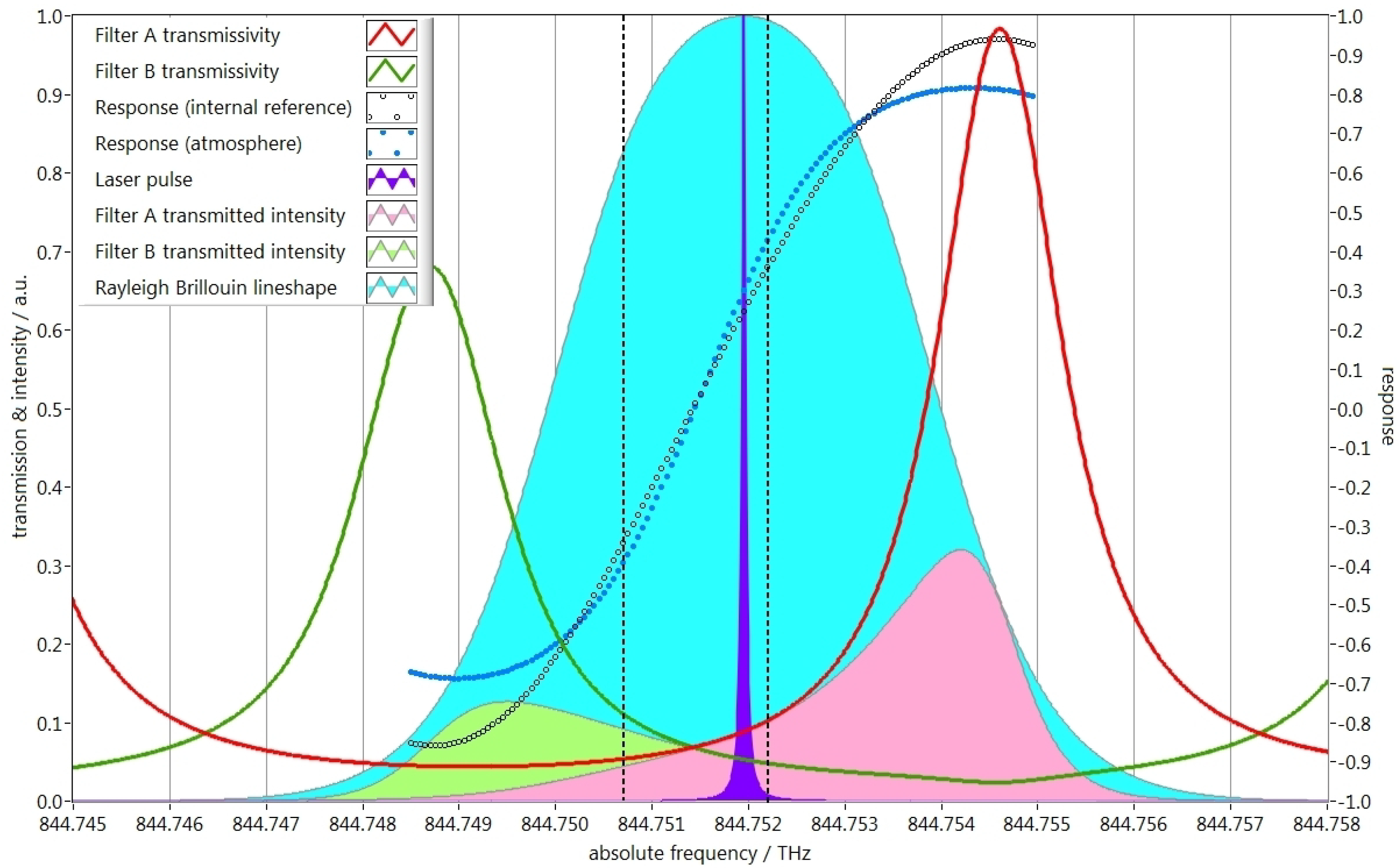
Figure 1 presents the direct-detection measurement principle applied to the molecular signal by the satellite instrument ALADIN and the A2D. The emitted laser spectrum is depicted as a narrow-band, violet peak with a full width at half maximum (FWHM) of 50 MHz. In contrast, the molecular Rayleigh backscatter spectrum is largely broadened up to about 4 GHz FWHM by thermal motion of the molecules. To the right and left of the Rayleigh spectrum the transmissivities of the two FPIs are indicated by a red and green line along with their corresponding transmitted intensities I(A) and I(B) symbolized by the pink and lime green filled areas. As described in Garnier and Chanin [53] a so-called Rayleigh response R${}_{\mathrm{R}}$ can be calculated as the contrast ratio from the two intensities transmitted through filter A and B depending on the frequency f.

$$R_{\mathrm{R}}\left(f\right)=\frac{I_{\mathrm{A}}\left(f\right)-I_{\mathrm{B}}\left(f\right)}{I_{\mathrm{A}}\left(f\right)+I_{\mathrm{B}}\left(f\right)}$$

(1)

The response describes the relation between the received backscatter signal and the frequency. Respective calibration curves are obtained by tuning the laser over a wide frequency range of at least 1 GHz and determining the response as depicted for the Internal Reference (black circles) and atmospheric signal (dotted dark blue line) in Figure 1. Among others, the shape of the response curves depends on the spectral width of the spectrum of the backscatter signal and the frequency spacing between the two filters.

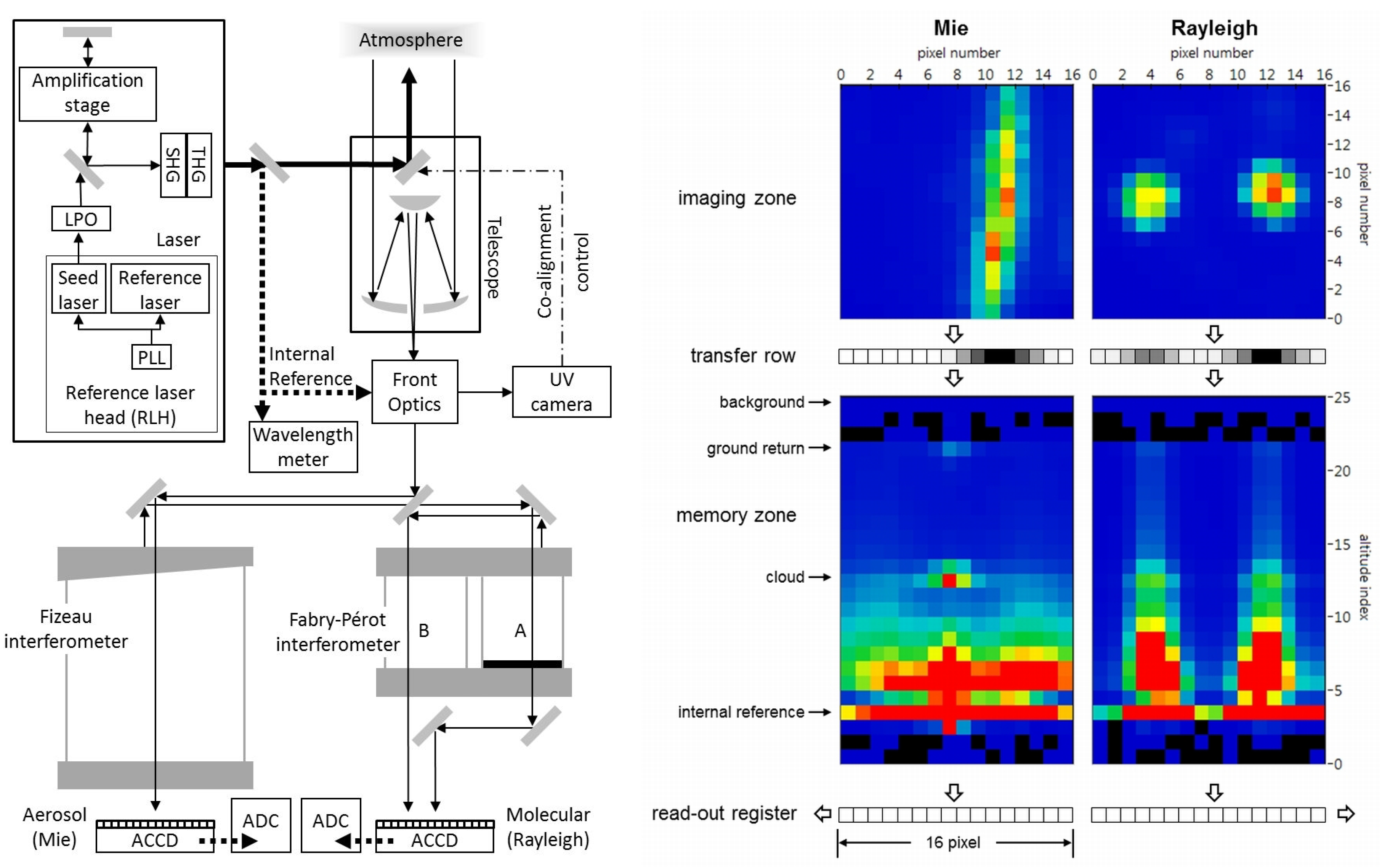
On the left of Figure 2 the structure of the A2D and its subsystems is illustrated. The laser of the A2D is set up in a master-oscillator power-amplifier configuration using two identical continuous wave lasers in the Reference Laser Head (RLH), one acting as seed laser for the oscillator, the other one as reference laser at 1064 nm (Lemmerz et al. [40]). Whereas the frequency of the reference laser is kept constant, the seed laser provides tunability. By optically beating the two frequencies, the frequency difference between both lasers can be controlled via a Phase Locked Loop (PLL) and set to a user-defined offset. This capability permits tuning over a frequency range of ≈12 GHz (UV) and constitutes the basis for the response calibration procedure (Figure 1). After having passed the Low Power Oscillator (LPO), the amplification stage as well as the second (SHG) and third (THG) harmonic generator crystals, the UV laser pulse is released towards the atmosphere showing a short-term frequency stability and linewidth of 3 MHz (rms) and 50 MHz, respectively, at 355 nm (Lemmerz et al. [40]). Part of the emitted laser pulse is redirected for Internal Reference measurements and for monitoring its exact wavelength via a wavelength meter (High Finesse WSU-10 or WSU-2). At a laser emission frequency in the UV of 844.5 × 10${}^{12}$ Hz (i.e., a wavelength of 354.8 nm), a relative velocity of 1 m/s along the LOS results in a Doppler shift of 5.63 MHz. Here, we use the factor k = 5.63 MHz/(m/s) to convert from frequency to velocity or vice versa. Consequently, the LiDAR system must be capable of detecting such a small frequency shift to ensure a wind measurement accuracy of 1 m/s. With the Rayleigh spectrum being more than 300 times broader and a Mie channel resolution of ≈17 m/s per pixel, this poses an enormous challenge. Therefore, the detection of photons must operate close to the shot noise limit which could be achieved by employing a novel ACCD technology. Another new design aspect applied in the ALADIN payload and the A2D is a sequential arrangement of Mie and Rayleigh receiver that can separate the signals from particle and molecular backscatter, allowing for two different ways of wind retrieval (Reitebuch [36]). Also, the sequential arrangement of the FPIs constitutes a unique feature and allows the reuse of the reflected light from the first FPI for the second one. The intensities transmitted through the interferometers are acquired by a light-sensitive imaging zone of the ACCDs (Figure 2, right). Whereas the Fizeau wedge of the Mie channel forms a linear fringe, the FPIs produce two spots with fixed positions. The vertically summed intensities of the imaging zone are shifted via a transfer row to the memory zone whose 25 rows correspond to the range-gates of the atmospheric measurements of ALADIN including one range-gate dedicated to the solar background measurement. For the A2D, only 21 range-gates are available for atmospheric measurements. The first four range-gates are dedicated to the measurement of the Internal Reference and the detection chain offset (DCO). As indicated in the memory zone, lateral shifts of position of the fringe peak position as well as a changing intensity ratio of the spots then relate to the same frequency shift.

3. Campaigns and Datasets

Together with the 2-µm coherent system, the A2D was employed during three airborne campaigns: in 2009 and 2015 dedicated to Aeolus validation purposes and in 2016 within the context of the NAWDEX campaign (Lux et al. [45]). Based in Keflavik, Iceland, the two LiDARs on-board the DLR Falcon 20 aircraft covered a large part of the North Atlantic region (Figure 3). As listed in

Table 1. Overview of the flights conducted during the airborne campaign in 2009. KEF: Keflavik, LPL: Liverpool, OBF: Oberpfaffenhofen, SFJ: Kangerlussuaq.

Flight No.	Date	Period (UTC)	Duration	Routeing	Objective/Comment
01	16.09.	10:06–12:46	2 h 40 min	OBF-OBF	test flight
02	18.09.	09:00–11:58	2 h 58 min	OBF-LPL	transfer flight part 1
03	18.09.	13:43–16:23	2 h 40 min	LPL-KEF	transfer flight part 2
04	21.09.	09:55–13:30	3 h 35 min	KEF-SFJ	2 calibrations over Greenland
05	21.09.	14:30–16:14	1 h 44 min	SFJ-KEF	wind measurements
06	25.09.	13:51–16:10	2 h 19 min	KEF-KEF	very cloudy, Mie winds only
07	26.09.	10:43–13:52	3 h 09 min	KEF-SFJ	wind measurement, jet stream
08	26.09	14:34–18:10	3 h 36 min	SFJ-KEF	sea surface reflectance at various angles
09	29.09.	10:57–14:55	3 h 58 min	KEF-KEF	wind measurement, different reference position
10	01.10.	08:56–12:50	3 h 54 min	KEF-OBF	transfer flight, broken clouds

and

Table 2. Overview of the flights conducted during the airborne campaign in 2015. GL: Greenland, GS: Greenland summit, KEF: Keflavik, OBF: Oberpfaffenhofen, PIK: Prestwick, SFJ: Kangerlussuaq.

Flight No.	Date	Period (UTC)	Duration	Routeing	Objective/Comment
01	11.05.	08:12–10:46	2 h 34 min	OBF-PIK	transfer flight part 1
02	11.05.	12:30–14:49	2 h 19 min	PIK-KEF	transfer flight part 2
03	13.05.	10:57–13:40	2 h 43 min	KEF-KEF	TDS-1 satellite underpass
04	15.05.	16:02–20:12	4 h 10 min	KEF-PIK-KEF	jet-stream measurements
05	16.05.	13:55–17:20	3 h 25 min	KEF-SFJ	2 calibrations over Greenland
06	16.05.	18:12–21:13	3 h 01 min	SFJ-KEF	1 calibration over Greenland
07	19.05.	11:59–15:46	3 h 47 min	KEF-GL-KEF	Greenland tip jet & rehearsal of Aeolus underpass
08	21.05.	22:29–02:26	3 h 57 min	KEF-GS-KEF	Greenland summit station
09	23.05.	16:54–21:10	4 h 16 min	KEF-GL-KEF	2 calibrations over sea ice
10	25.05.	14:05–17:20	3 h 15 min	KEF-KEF	Iceland & southerly jet
11	28.05.	10:23–13:25	3 h 02 min	KEF-KEF	ASCAT satellite underpass & rehearsal of Aeolus underpass
12	29.05.	10:09–12:39	2 h 30 min	KEF-PIK	transfer flight part 1
13	29.05.	13:55–15:54	1 h 59 min	PIK-OBF	transfer flight part 2

, 10 and 13 flights were completed in 2009 and 2015, respectively, seven of which being transfer flights from and to DLR Oberpfaffenhofen, Germany. The tables give an overview of the date, the period and the duration complemented by information about the routing and the main objective of each flight. Hereby, the duration comprises the time between take-off and landing. Due to warm-up phases of the A2D and flight safety restrictions, the actual operation time of the LiDAR was shorter. Additionally, parts of the operation time of the A2D were spent on modes other than wind measurement, such as response calibration, instrument spectral registration or background calibration. In May 2015, twenty-one flight legs with continuous A2D wind measurements lasting at least 10 min were conducted, the longest being almost 88 min. Overall, this adds up to more than 12 h of valuable wind data compared to about 41 flying hours. Apart from the actual wind measurements, the objectives ranged from, e.g., the performance of response calibrations over the determination of sea surface reflectance to the rehearsal of satellite underpasses. In the following, we focus on the detailed analysis and comparison of the A2D IRCs which must pass strict quality controls to minimize errors that can potentially be passed on to the wind measurements. In particular, low systematic errors are a prerequisite for further consideration in NWP models.

4. Instrument Response Calibration

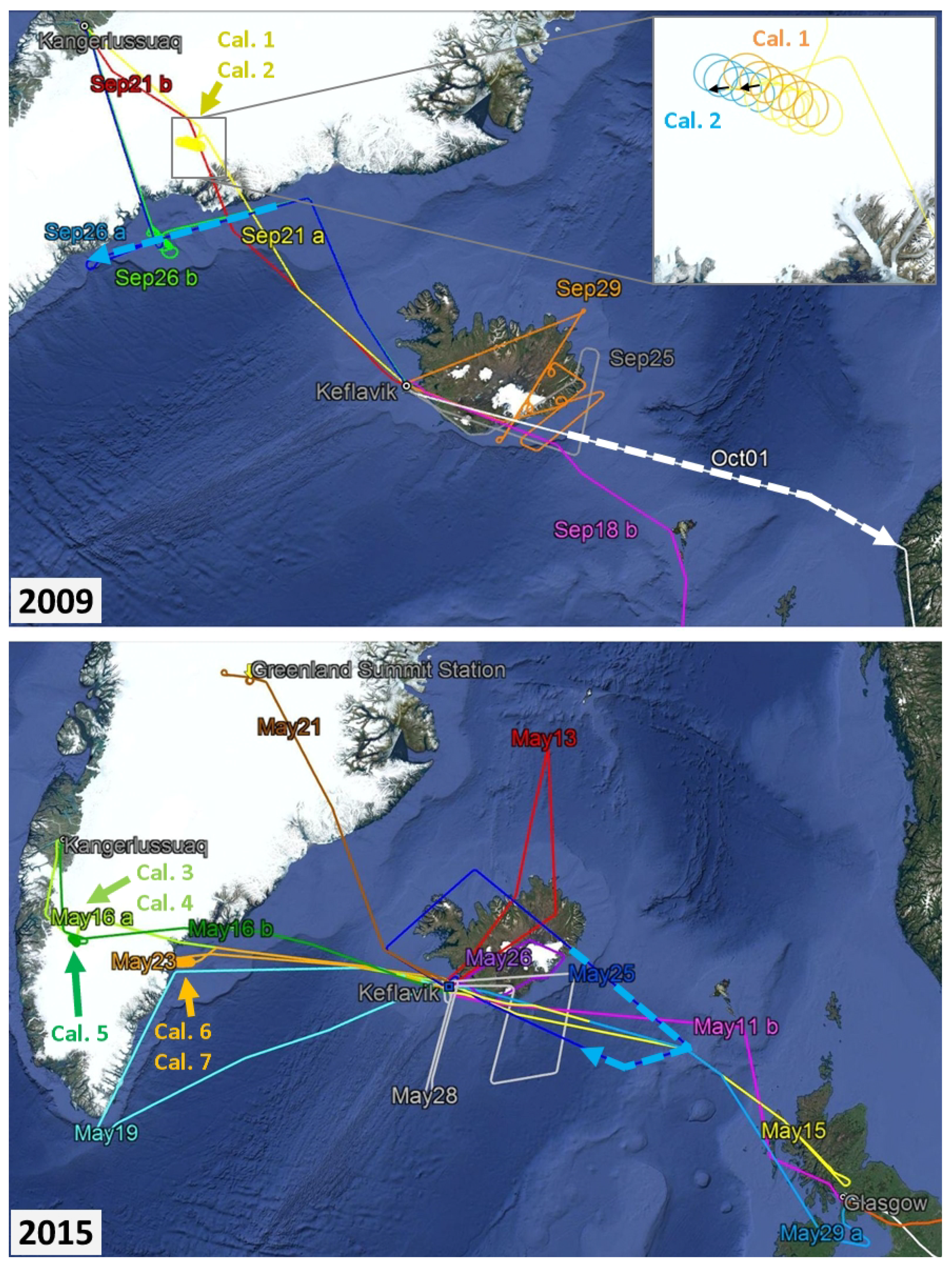
According to the method explained along with Figure 1 seven instrument response calibrations could be obtained under constant atmospheric and cloud-free conditions during the two airborne campaigns in 2009 and 2015 (Figure 3,

Table 3. Overview of the A2D instrument response calibrations (IRCs) conducted during the airborne campaigns in 2009 and 2015.

IRC No.	Date	Period (UTC)	Location
1	21.09.	11:24–11:47	over Greenland ice sheet
2	21.09.	11:57–12:19	over Greenland ice sheet
3	16.05.	15:34–15:57	over Greenland ice sheet
4	16.05.	16:06–16:30	over Greenland ice sheet
5	16.05.	18:54–19:18	over Greenland ice sheet
6	23.05.	18:21–18:44	over sea ice off the south-east coast of Greenland
7	23.05.	18:50–15:12	over sea ice off the south-east coast of Greenland

). A reliable response calibration derived from strong and preferably continuous ground return signal is required for the Mie wind retrieval in particular but also for possible bias corrections in both channels. In this respect the Greenland ice shield and the sea ice close to the coast provided favorable conditions due to the high surface albedo of ice in the UV. In order to obtain an instrument response function, the frequency of the A2D laser is changed in steps of 25 MHz over a range of 1800 MHz. For comparison, the frequency range of an ALADIN response calibration comprises only 40 steps within 1000 MHz, due to the electrical power restrictions that allow the satellite to stay in nadir-pointing mode for not much longer than about 20 min.

Nadir pointing allows to avoid Doppler shifts induced by the velocity of the moving platform along the LOS direction or the horizontal wind speed in the probed atmospheric volume, thereby assuring the exclusive dependency of the instrument response on the emitted frequency during an IRC. Thus, the Falcon aircraft needs to fly right-hand bends of 20${}^{\circ }$ to compensate for the off-nadir viewing angle of the A2D (see inset of Figure 3). Easterly wind constantly pushed the aircraft towards the coast, resulting in cycloid shapes of the flight track. At nadir pointing, we additionally assume that the influence of vertical wind speeds is negligible over the time of a calibration, i.e., ≈20 min for the A2D and 16 min for Aeolus. With a speed of 200 m/s of the Falcon, the covered distance amounts up to 240 km (or an area of roughly 40 km times 70 km in Figure 3) compared to almost 7000 km for the satellite flying at 7.2 km/s. Vertical winds are encountered in convective conditions and during gravity wave events (Witschas et al. [16]). Accordingly, the flight planning for the A2D IRCs aims at cloud-free areas without convection. While under optimal conditions the A2D can perform about two IRCs per hour or six per research flight, the Aeolus satellite will presumably be commanded to conduct an IRC only once per week, preferably over the Arctic and Antarctica.

An IRC consists of a Rayleigh response calibration (RRC) and a Mie response calibration (MRC) always performed in parallel while distributing the backscattered light onto the spectrometers according to Figure 2 (left). At every frequency step of an A2D IRC, the signals from the Internal Reference, the atmosphere and the ground returns are accumulated over n = 700 pulses. While doing so, subgroups of usually 20 pulses at a time are summed up to an intermediate fragmentation of m = 35 measurements. With a laser repetition frequency of 50 Hz and an idle time of 4 s, one step lasts 18 s, defined as an observation o. In contrast, the accumulation time of a calibration step for Aeolus is 24 s, consisting of two observations with a duration of 12 s each and no idle time. The numbering of the A2D range-gates i ranges from #0 - #24. 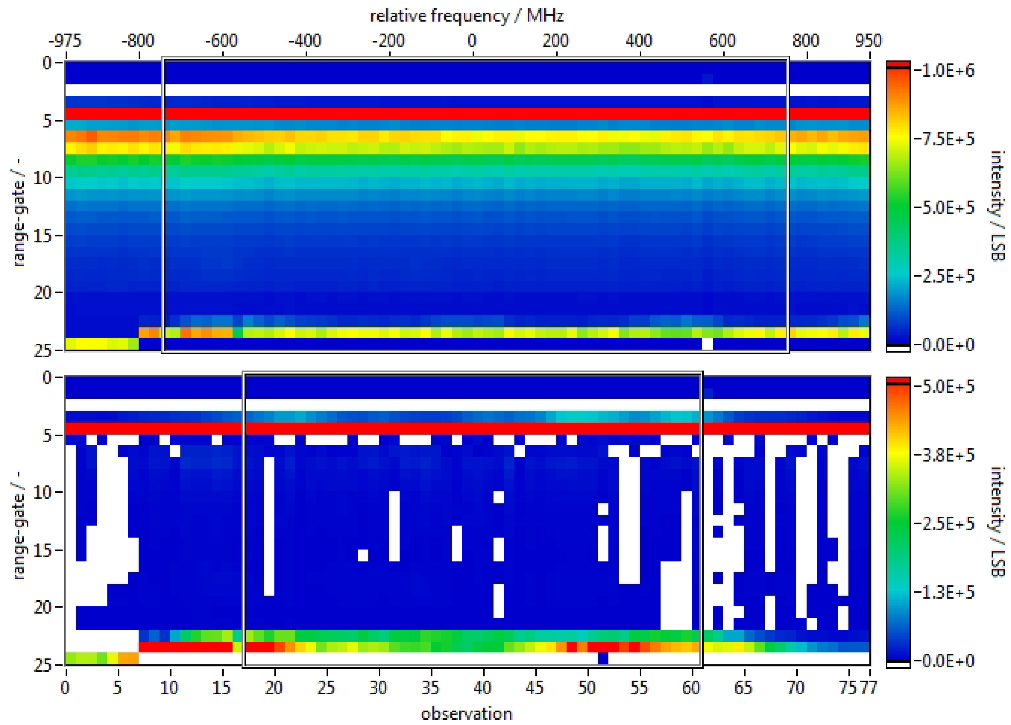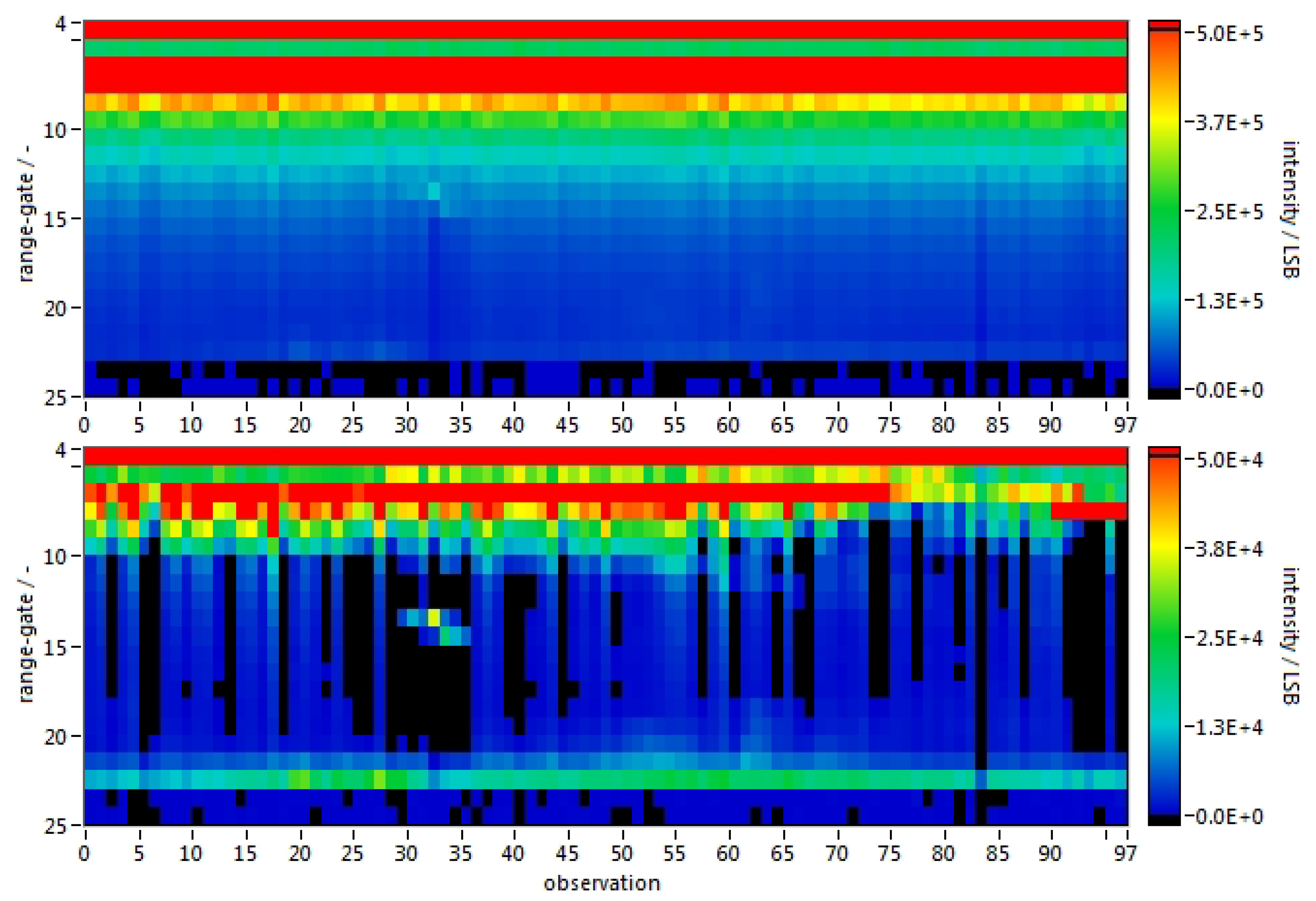Figure 4 shows the measured intensities during IRC #7 per observation for all 25 range-gates in the Rayleigh channel and the Mie channel. The first five range-gates are dedicated to the measurement of the background signal in the 0th range-gate, the DCO in the 2nd range-gate and the Internal Reference in range-gate #4. Range-gates #1 and #3 are used as buffers towards the Internal Reference and the solar background range-gates to assure undisturbed DCO measurements. The DCO, which emanates from a voltage offset before digitization, is determined as an average over p = 16 pixels according to Equation (2).

$$I_{\mathrm{DCO}}\left(m\right)=\frac{1}{16}\sum _{p=1}^{16}{I}_{\mathrm{raw}}(p,m,i=2)$$

(2)

Here, I${}_{\mathrm{raw}}$ is the raw intensity recorded by pixel number p within the 2nd row of the memory zone (Figure 2) for the mth measurement of an observation. The background signal for each atmospheric range-gate is obtained from the 0th range-gate according to Equation (3) by first subtracting the DCO before scaling the resulting intensity by the ratio of the integration times of the ith range-gate and the 0th range-gate, i.e., the background range-gate. Whereas typical integration times of the atmospheric range-gates range from 2.1 $\mathsf{\mu }$s (≈315 m in range) to 16.8 $\mathsf{\mu }$s (≈2500 m in range), the solar background signal is usually obtained over an accumulation time of 8333 $\mathsf{\mu }$s.

$$I_{\mathrm{BKG}}(p,m,i)=[I_{\mathrm{raw}}(p,m,i=0)-I_{\mathrm{DCO}}\left(m\right)]·\frac{t_{\mathrm{i}}}{t_0}$$

(3)

After subtracting the DCO and the background from the Internal Reference and the atmospheric raw intensities according to Equations (4a) and (4b), one obtains the actual signals I${}_{\mathrm{INT}}$ and I(i) per range-gate i.

$$\begin{array}{cc}\hfill I\left(i\right)& =\sum _{m=1}^{35}\sum _{p=1}^{16}[I_{\mathrm{raw}}(p,m,i)-I_{\mathrm{DCO}}\left(p\right)-I_{\mathrm{BKG}}(p,m,i)]\hspace{1em}\hspace{1em}i=5,\dots ,24\hfill \end{array}$$

(4a)

$$\begin{array}{cc}\hfill I_{\mathrm{INT}}& =\sum _{m=1}^{35}\sum _{p=1}^{16}[I_{\mathrm{raw}}(p,m,i=4)-I_{\mathrm{DCO}}\left(p\right)]\hfill \end{array}$$

(4b)

The intensities are measured in digitizer counts, so-called least-significant bits (LSB), which emanate from the conversion of signal electrons within the ADC. Equations (2)–(4b) are valid for both the Mie and the Rayleigh channel. Whereas Equations (4a) and (4b) are equivalent to the Rayleigh intensities presented in Figure 4, an additional step was inserted for the Mie intensities by subtracting the Rayleigh background on the Mie channel. The broadband molecular backscatter appears as a rather constant offset within the narrow useful spectral range ((Reitebuch et al. [30])) of the Mie channel and is determined via a dedicated procedure during which the laser frequency is tuned out of this useful spectral range, that is the Mie fringes are not visible on the ACCD as depicted in Figure 2. White areas in the atmospheric range-gates of the Mie intensities in Figure 4 are caused by variations of the molecular background on the Mie channel and the related uncertainty. The high intensities present in range-gate #4 of both channels, correspond to the Internal Reference located at flight altitude of the Falcon aircraft of ≈10.1 km. An electro-optical modulator blocks most of the strong signal from the first atmospheric range-gate #5 preventing the ACCD from saturation. From range-gate #6 downward, the quadratic range dependency is well visible in the continuous decrease of the received intensity, particularly in the Rayleigh channel. The sea ice return is prominently located in range-gate #23 and partly in range-gate #22. After observation #7 range-gate #24 lies below the ground showing just random electric noise. Apart from the ground, no obvious features, such as enhanced backscatter from clouds or aerosol layers, appear in the atmospheric signal of the Mie and Rayleigh channel. This shows that IRC #7 was conducted in a clear atmosphere and the evaluated RRC curves are not affected by cross-talk effects.

The grey boxes in Figure 4 indicate the frequency intervals used to determine the characteristics of the response curves: 1500 MHz, i.e., 60 steps or observations, for the Rayleigh channel and 1100 MHz, i.e., 44 steps or observations, for the Mie channel.

Based on the raw intensities per measurement m, Equations (4) and (5) combined in Equation (1) give the Rayleigh responses R${}_{\mathrm{R},\mathrm{o},\mathrm{i}}$ per range-gate i and per observation o, i.e., per frequency step. In contrast to the FPI, where a frequency shift causes a change in transmitted intensities, this shift manifests itself as a change of the lateral position of the Mie fringe formed by the Fizeau interferometer (Figure 2). The Mie response R${}_{\mathrm{M},\mathrm{o},\mathrm{i}}$ is then equivalent to the pixel position $\widehat{x}$(f) of the centroid of the detected fringe (Equation (6)) which is determined via the Downhill Simplex fitting algorithm (Nelder and Mead [54]; Press et al. [55]) to fit a Lorentzian function to the filter function (Paffrath et al. [39])).

The center of the Mie interval corresponds to the frequency where the position of the fringe leads to equal intensities on pixel #7 and #8 in the integrated ACCD signal. In a co-registration process, the so-called Rayleigh filter crosspoint is shifted to the Mie center frequency by adapting the temperatures of the FPI. The filter crosspoint is defined as the point in the Internal Reference where I${}_{\mathrm{A},\mathrm{o},4}$ = I${}_{\mathrm{B},\mathrm{o},4}$ (Equation (5)) and hence R${}_{\mathrm{R},\mathrm{o},4}$ = 0 according to Equation (1). The considered frequency interval for the Rayleigh channel of 1500 MHz (also indicated in Figure 1) is selected symmetrically around this crosspoint.

$$\begin{array}{cc}\hfill I_{\mathrm{A},\mathrm{o},\mathrm{i}}& =\sum _{m=1}^{35}\sum _{p=1}^6[I_{\mathrm{raw}}(p,m,i)-I_{\mathrm{DCO}}\left(m\right)-I_{\mathrm{BKG}}(p,m)]\hfill \end{array}$$

(5a)

$$\begin{array}{cc}\hfill I_{\mathrm{B},\mathrm{o},\mathrm{i}}& =\sum _{m=1}^{35}\sum _{p=9}^{14}[I_{\mathrm{raw}}(p,m,i)-I_{\mathrm{DCO}}\left(m\right)-I_{\mathrm{BKG}}(p,m)]\hfill \end{array}$$

(5b)

$$R_{\mathrm{M},\mathrm{o},\mathrm{i}}=\widehat{x}\left(f\right)$$

(6)

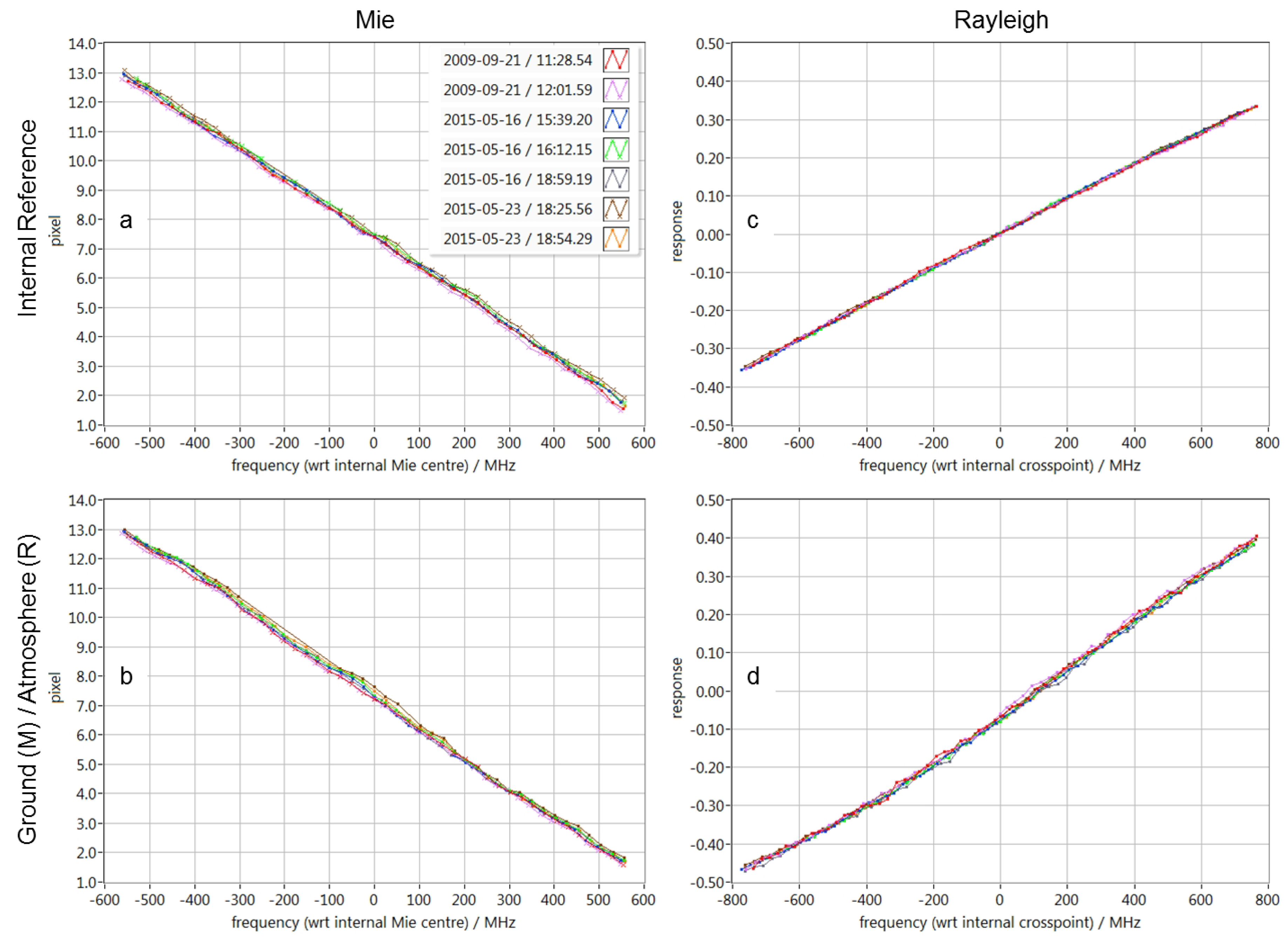
An additional correction is applied to the resulting responses at the observation level with respect to the error induced by the motion of the moving platform. Seven instrument response functions each are displayed in Figure 5 for the Internal Reference of the Mie (top left) and Rayleigh channel (top right) as well as for the Mie channel ground return signal (bottom left) and the atmospheric molecular signal from range-gates 4.7 km from the aircraft (bottom right), corresponding to a mean altitude of 5.2 km. For convenience, the x-axes use relative rather than absolute frequencies measured by a wavemeter. Depending on the considered channel, the reference frequency at 0 MHz corresponds to the Mie center or to the Rayleigh filter crosspoint, respectively. With a sensitivity of about 100 MHz per pixel in the Mie channel, the ACCD width of 16 pixels is suitable for measurements within a frequency range of a maximum of 1600 MHz. However, a range of ±550 MHz is sufficient for our analyses and avoids strong non-linear effects when determining the fringe position at the edges of the ACCD. Due to the concept of measuring intensities, the Rayleigh channel is less restricted and permits the use of a range of ±750 MHz (±133 m/s). The atmospheric Rayleigh response functions presented in Figure 5 are derived from range-gates of 630 m vertical thickness, 4.7 km from the instrument. Details about the analysis of A2D ground returns and in particular the respective response functions can be found in Weiler [56] and Lux et al. [45] where improvements on the ground detection algorithm are discussed which became necessary during the analysis of the NAWDEX campaign in 2016, but were not applied here.

While for the Internal Reference and the ground return, one response function each is obtained from the RRC and the MRC, the Rayleigh channel also allows response functions to be derived per atmospheric range-gate. Due to the narrow spectral width of the ground return signal being similar to that of the atmospheric backscatter by aerosols and clouds, the Mie response function of the ground return can be used to retrieve atmospheric wind speed. In contrast, the largely different spectral widths of the Rayleigh atmospheric and ground return signal lead to different transmitted intensities and hence shapes of the response functions, finally requiring dedicated response functions in the wind retrieval. For both channels, precise knowledge of the ground return response function is needed to correct for system inherent biases via a so-called zero wind correction, where the non-moving ground serves as a wind speed reference. In this respect, biases on whole assimilated wind curtains can be very detrimental for NWP (Horányi et al. [57]). The compilations presented in Figure 5 reveal only minor variations in the shapes of the response functions despite almost six years in between their recording. This underlines the long-term stability of the A2D system.

As discussed along with Figure 1, the response R${}_{\mathrm{R}}$ depends on the spectral width of the molecular backscatter, i.e., on the temperature and pressure of the probed atmospheric volume (Witschas et al. [52]; Witschas et al. [58]). The fact that for the A2D, one calibration curve per atmospheric range-gate is derived from the RRC renders the wind retrieval less sensitive to pressure than to temperature, considering the usually encountered variations. In contrast, for Aeolus, the signal from the whole altitude range between, e.g., 6 km to 16 km, is merged into only one single RRC curve. Since IRC and wind measurement cannot be performed at the same time and mostly do not take place at the same location, the encountered temperature and pressure differences cause variations in the assignment of response to frequency (Figure 5) and, hence, in the determined wind speed. For the A2D airborne campaigns in 2009 and 2015, the resulting systematic and random errors are negligibly small compared to other error sources such as the co-alignment or speckle noise on the Internal Reference. However, the systematic error in particular becomes significant for temperature differences of several tens of degrees between the locations of the IRC and the wind measurement. Appropriate corrections with respect to temperature and pressure described by Dabas et al. [59] have been integrated into the Aeolus Level 2B processor (Tan et al. [60]). In contrast to the airborne system which circles over almost the same area during an IRC (see inset of Figure 3), an IRC of Aeolus stretches over about 7000 km preferably above the Arctic or Antarctic ice sheets, entailing respective temperature and pressure variations in the atmosphere not only on the vertical but also on the horizontal scale.

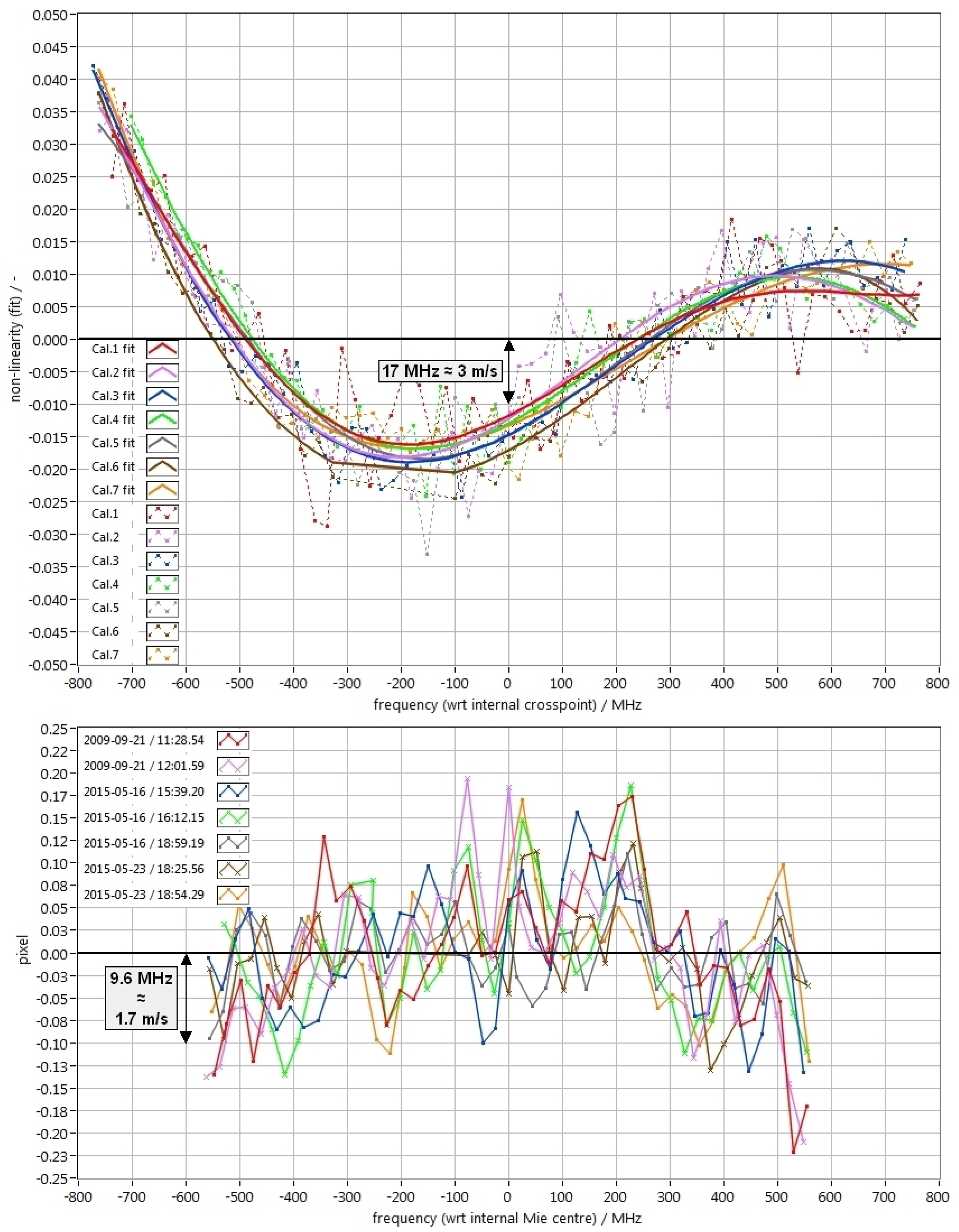
Subtracting linear fits from the response functions in Figure 5 reveals the structure of their non-linearities in more detail (Figure 6). In contrast to the Mie response functions, which can be well described by linear fits, the Rayleigh response functions require a higher order fit to mimic their slightly undulated shape with sufficient accuracy. This is especially the case for the molecular signal from the atmosphere which exhibits a much broader spectral width than the Internal Reference. Currently the Rayleigh response functions are approximated by a 5th-order polynomial fit via an LU (lower-upper) decomposition algorithm (Press et al. [55]). In particular, the odd order of the polynomial takes into account the seemingly point-symmetric shape of the response functions with their sole inflection point. Polynomial orders lower than 5 could not reproduce the shape of the response functions well enough whereas higher orders tended to introduce non-meaningful oscillations. Additionally, the fits by 5th-order polynomials lead to reasonably low residual errors (Figure 7). More information is available in Marksteiner [61].

$$R_{\mathrm{R}}\left(f\right)=\sum _{i=0}^5(c_{\mathrm{i}}·f^i)$$

(7)

The polynomial coefficients c${}_{\mathrm{i}}$ from Equation (7) are compiled in

Table 4. Coefficients c${}_i$ derived from a 5th-order polynomial fit through the Rayleigh response functions of the Internal Reference (INT), the atmospheric (ATM) at a distance of 4.7 km from the instrument together with the mean and the peak-to-peak value $\delta$ over the coefficients from all calibrations.

IRC no.	c${}_0$/10${}^{-3}$	c${}_1$/10${}^{-4}$ MHz${}^{-1}$	c${}_2$/10${}^{-8}$ MHz${}^{-2}$	c${}_3$/10${}^{-11}$ MHz${}^{-3}$	c${}_4$/10${}^{-14}$ MHz${}^{-4}$	c${}_5$/10${}^{-17}$ MHz${}^{-5}$
Internal Reference
1	4.59	4.44	−3.45	4.20	2.09	−5.57
2	4.20	4.64	−2.56	−9.83	−0.16	13.47
3	2.61	4.69	−1.02	−4.88	−2.33	4.12
4	4.33	4.72	−2.36	−6.17	0.05	4.72
5	1.39	4.65	−0.29	−3.37	−3.07	1.09
6	3.52	4.57	1.25	0.35	−4.99	−3.70
7	2.91	4.63	−1.39	−0.93	−1.55	−2.94
Atmosphere
1	−66.27	6.32	6.90	−17.55	−2.12	12.01
2	−62.19	6.44	7.44	−18.83	−3.68	10.25
3	−76.03	6.21	8.15	−12.88	−2.42	3.89
4	−74.58	6.28	8.69	−16.00	−4.53	6.73
5	−80.29	6.24	10.03	−15.83	−7.12	9.44
6	−67.34	6.25	8.56	−11.16	−3.68	−0.64
7	−71.91	6.18	6.55	−10.11	0.49	1.23

. The linear shape of the Mie response functions can be described by

$$R_{\mathrm{M}}\left(f\right)=c_{0,\mathrm{M}}+c_{1,\mathrm{M}}·f$$

(8)

with c${}_{0,\mathrm{M}}$ and c${}_{1,\mathrm{M}}$ being the intercept and the slope (or sensitivity) compiled for the individual IRCs in

Table 5. 0th (intercept) and 1st order (slope) coefficients derived from linear fits through the Mie response functions for the internal reference and the ground return. Additionally, the intercept difference between internal reference (INT) and ground return (GR) is provided. The mean values describe the average slope and intercept over the seven IRCs. The peak-to-peak difference is denoted as $\delta$.

IRC no.	Intercept/pixel	Slope/(pixel·GHz${}^{-1}$)	Intercept: INT-GR/pixel
Internal Reference
1	7.32	−10.08
2	7.22	−10.10
3	7.37	−10.00
4	7.45	−10.08
5	7.38	−10.07
6	7.54	−10.01
7	7.40	−10.08
mean	7.38	−10.06
$\delta$	0.32	0.1004
Ground Return
1	7.23	−10.24	0.09
2	7.17	−10.27	0.05
3	7.26	−10.33	0.11
4	7.35	−10.37	0.10
5	7.28	−10.36	0.10
6	7.44	−10.34	0.10
7	7.37	−10.39	0.03
mean	7.30	−10.33	0.08
$\delta$	0.27	0.1501	0.08

.

Obviously, the values of the coefficients in Table 4 become smaller with increasing order of the coefficient (i.e., smallest values for c${}_5$). The higher the order of the coefficient, the more sensitive it is with respect to slight changes either in the shape of the response curve or of individual response values. The coefficients of the fits are constantly monitored and coarse outliers (such as the large c${}_5$ for the Internal Reference of IRC #2) can indicate issues with an IRC that result in slightly different characteristic of the response function. Among others, such information can be consulted to assess the quality of a specific response function in comparison to other response functions. However, the IRCs undergo an already strict quality control before being fitted, so that in most cases the outliers cannot be traced back to a certain root cause anymore. Certain patterns become apparent in Table 4 such as a predominant sign or an order of magnitude for each coefficient. For instance, the 6th RRC is the only one showing a c${}_2$ coefficient with a positive sign for the Internal Reference (1.25 × 10${}^{-8}$ MHz${}^{-2}$). Another example would be the by far largest c${}_1$ coefficient (slope) found for the atmosphere from the 2 th RRC (6.44 × 10${}^{-4}$ MHz${}^{-1}$). Regarding coefficient c${}_0$, which represents the intercept, large relative differences for the Internal Reference in Table 4 can emanate from changes in the temperature setting of the Rayleigh spectrometer. However, this will not affect the resulting wind speed as the wind speed is derived as a difference to the atmospheric response, which in turn is affected by the same temperature change.

Considering the conversion factor k and a mean slope for the Mie Internal Reference of −10.06 pixel/GHz, the according $\delta$ of 0.32 pixels translates into 5.65 m/s. This difference between the response functions cannot directly be interpreted as an equivalent difference in the final wind speeds. Instead, the wind retrieval uses the differential information between Internal Reference and ground return response function. The intercepts of the ground return show the same pattern as those of the Internal Reference, that is, for instance, the largest intercept is found for IRC #6 and the smallest for IRC #2, and with a mean slope of −10.33 pixel/GHz the $\delta$ of the ground return of 0.27 pixels corresponds to 4.64 m/s. Thus, the expected bias variation between wind speeds obtained from the same wind measurement but with different Mie response functions is assumed to be in the order of less than 1 m/s.

The application of a 5th-order polynomial fit to model the shape of the Rayleigh response function is an approximation based on an empirical approach. Regarding the Mie channel, fairly regular undulations can be observed in Figure 6 that are assumed to be related to the special layout of the ACCD being based on 16 × 16 pixels. With the width of 1 pixel being equivalent to about 100 MHz or 17 m/s LOS wind speed, the random structure of the Mie non-linearity function can cause errors, depending on the actually measured wind speed, i.e., fringe position. The implementation of an adequate, more sophisticated, fitting procedure (apart from the linear fit) for the Mie non-linearity part is currently being investigated. As confirmed by analyses of data from a current airborne campaign, a third order polynomial fit significantly reduces the standard deviation of the Mie residual error at a first step.

The ability of the A2D to perform IRCs over an increased frequency range of about 1.8 GHz compared to the 1 GHz of Aeolus, brings the advantage of more stable coefficients determining the shape of the response functions. However, Table 4 and Table 5 still show variation of the individual coefficients. Reasons can be found in the dominant known noise sources such as the Poisson noise and speckle noise but also in the variations in the co-alignment of the outgoing laser beam and telescope viewing direction, the uncertainty in the frequency measurement or the imprecise localization of the crosspoint, that have been verified in an extensive noise study (Witschas et al. [62]). Speckle noise, in particular, affects the A2D measurements due to an optical fiber that guides the Internal Reference signal, whereas ALADIN features free path propagation of the laser beam.

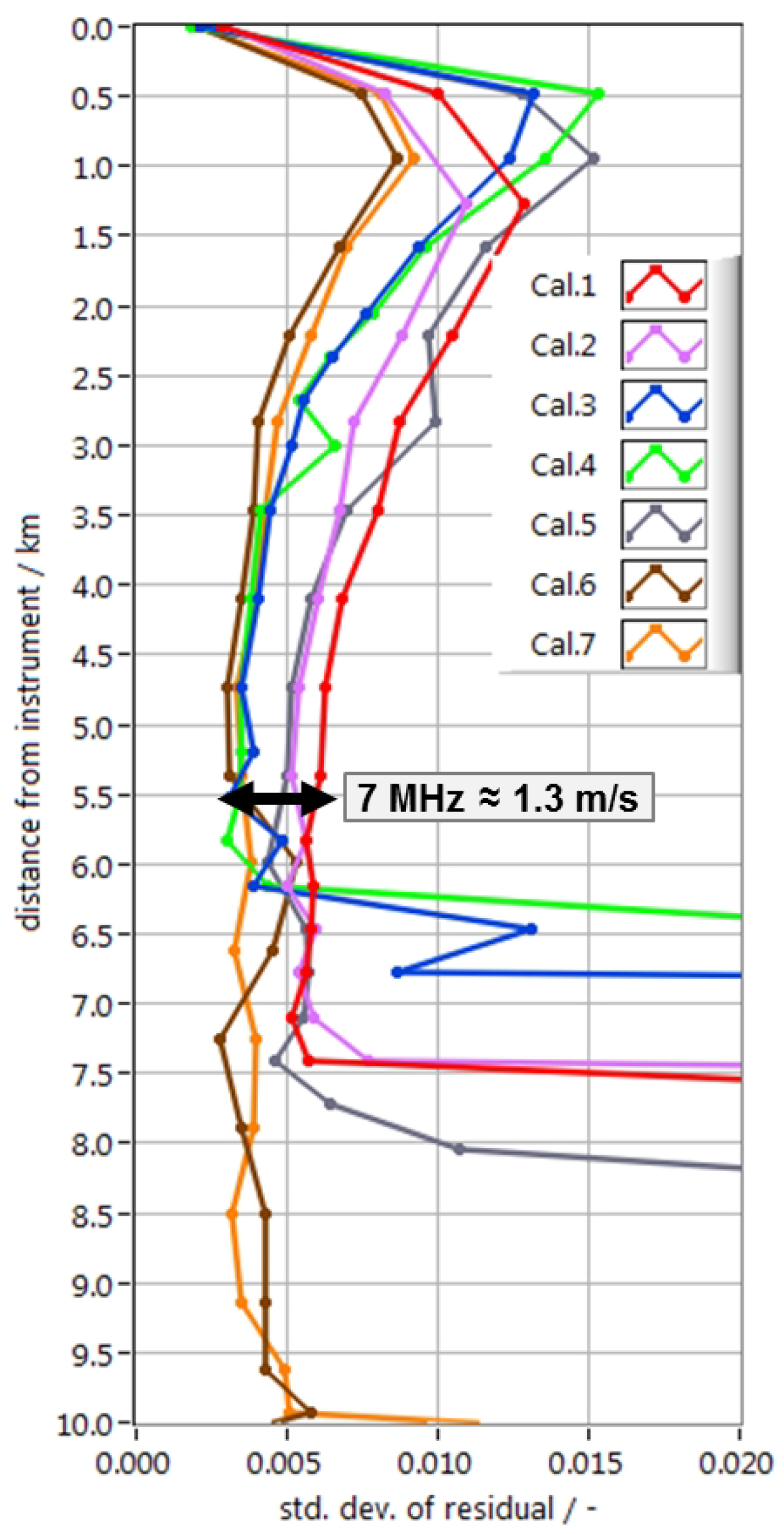
After subtracting fitted 5th-order polynomials from the RRC curves (Marksteiner [61]), residuals with rather random behavior remain. The standard deviation of these residuals is displayed for each range-gate in Figure 7. At the top, the Internal Reference shows the lowest standard deviation with response values between 0.0018 and 0.0029. This corresponds to 4.1 MHz and 6.4 MHz when, as a good first estimate, applying the mean slope of the Internal Reference response functions presented in Figure 5 of 0.454 GHz${}^{-1}$. Converted with the factor k, the resulting 0.72 m/s and 1.1 m/s, respectively, correspond to the remaining random error which is propagated from the response calibration of the Internal Reference towards the final wind speed measurements.

For all calibrations, a range dependency of the random error of the residual is visible, showing a maximum within the first atmospheric range-gates followed by an asymptotic approach towards a response value of around 0.004 with increasing distance from the instrument. Considering a mean slope of the Rayleigh atmospheric response functions (Figure 5d) of 0.582 GHz${}^{-1}$, this corresponds to 1.2 m/s. The gradient in the random error of the residual is mainly provoked by an interplay of laser beam pointing variations with the overlap function of telescope field-of-view and laser beam. As the FPI has been shown to be particularly sensitive to the variation of input angles (Witschas et al. [62]), it is essential that the co-alignment of the two optical axes of the telescope and outgoing laser beam (monostatic biaxial LiDAR) is optimized by a dedicated control loop. In addition, the electro-optic modulator is still partly closed during the acquisition time of the first atmospheric range-gate to protect the ACCDs from damage by reducing the strong backscatter intensity emanating from the near field. The mentioned effects render most of the retrieved wind measurements in the near field unusable, resulting in an exclusion of the first three atmospheric range-gates from scientific reasoning and statistical comparisons. In contrast, the winds obtained by Aeolus are not subject to such drawbacks since this satellite mission exclusively measures in the far-field on the one hand and features a monostatic coaxial transceiver on the other hand. Coming from flight heights of 8 km–10 km, the Greenland ice shield with altitudes of more than 3 km successively blocks the lowest range-gates between 6 km and 8 km distance from the instrument. Therefore, no data is available in that region except for calibrations #6 and #7 which reached down to the sea surface. At medium ranges of about 5 km, the standard deviation varies among the calibrations in the order of 7 MHz (1.3 m/s). Despite the mentioned stability of the A2D system, IRCs from 2009 cannot be used for wind retrieval from measurements recorded in 2015 and vice versa. Owing to differences in the alignment in between the two campaigns as well as to drifts during the individual campaigns, the characteristics of the response functions differ especially in the near field of the A2D, that is the region of incomplete telescope overlap within the first 2–3 km from the instrument (Figure 7).

5. Comparison of Instrument Response Calibrations

The differences between the response calibration curves presented above require quantification to assess the variability they inherit to the final wind speeds. Thus, according to Equation (9), we compute ‘virtual’ wind speeds v${}_{\mathrm{sim}}$ from the predefined identical frequency arrays for each IRC with ${\lambda }_0$ being the wavelength of the emitted laser pulses.

$$v_{\mathrm{sim}}\left(f\right)=(f_{\mathrm{ATM}}-f_{\mathrm{INT}})·\frac{{\lambda }_0}{2}$$

(9)

The f${}_{\mathrm{ATM}}$ and f${}_{\mathrm{INT}}$ constitute the frequencies resolved after inverting the respective Mie (ground return) and Rayleigh (atmospheric) response functions (Equations (7) and (8)) for the atmospheric and Internal Reference range-gates. Regarding the Rayleigh channel, that means determining the correct roots from the 5th-order polynomial. The ‘virtual’ winds are determined in uniform steps of 25 MHz (4.5 m/s) over the whole calibration ranges, i.e., ±550 MHz for the Mie and ±750 MHz for the Rayleigh channel, thereby imitating wind measurements between ±98 m/s and ±133 m/s, respectively. This approach based on simulated wind additionally allows to examine the behavior of the response functions over a wider frequency range than usually available from real measurements, where a range of ±100 MHz (18 m/s) is rarely exceeded.

Next, the derived v${}_{\mathrm{sim}}$ are compared for each pair of IRCs. When considering four of the five calibrations from 2015, this results in six pairs. Calibration #6 is disregarded here to avoid larger deviations caused by a temporal outage of the co-alignment control loop in the middle of the IRC. Subsequently, a mean value of the six differences at every frequency step is calculated resulting in the curve presented for the Mie channel in Figure 8 (right). Depending on the actually measured wind speed, a mean difference between 0.45 m/s and 0.85 m/s can be expected on average when processing the same wind field with two MRCs that are randomly selected from the set of those four. Considering usual LOS wind speeds measured by the A2D between ±25 m/s, being equivalent to about ±140 MHz, the expected uncertainty rather ranges between 0.5 m/s and 0.65 m/s. For the retrieval of Mie winds only a single instrument response function is available, which is derived from the ground return signal. Equivalently repeating the procedure for different atmospheric range-gates in the Rayleigh channel, results in the curves displayed in Figure 8 (left). Assuming a measurement at a distance of 6.2 km from the instrument in windless conditions, that is at 0 MHz frequency shift, the derived wind speed will differ, on average, by 0.7 m/s when running the wind retrieval algorithm with two randomly chosen RRCs (among the set of calibrations #3, #4, #5 and #7).

6. Wind Retrieval and Statistical Comparison

On 26 September 2009, the A2D performed wind speed measurements on a straight flight leg along the east coast of Greenland for almost 30 min, i.e., 1764 s or 98 observations (Figure 3, top). A basic view of the atmospheric conditions and structure is provided by the measured intensities per observation, summed over all 16 pixels for both the Rayleigh channel and the Mie channel in Figure 9 (Equation (4)). The high intensities present in range-gate #4 of both channels correspond to the Internal Reference located at the flight altitude of the Falcon aircraft. An electro-optical modulator blocks most of the strong signal from the first atmospheric range-gate #5 preventing the ACCD from saturation. From range-gate #6 downward, the continuous decrease of the received intensity, particularly in the Rayleigh channel, mainly results from the quadratic range dependency. In the Mie channel, the sea surface return is prominently located in range-gate #22 and partly in range-gate #21. The range-gates #23 and #24 lie below the ground, showing just random detection noise. Between observations 45 and 70, reaching from the sea surface up to range-gate #18, a katabatic flow coming down from the Greenland ice shield yields slightly higher backscatter intensity, likely due to transported ice and snow crystals and/or by dispersing sea salt (see Figure 11). Another prominent feature is a small cloud in range-gates #14 and #15 between observations 30 and 35, clearly visible in the Mie channel and indicated by its shadowing effect in the Rayleigh channel. Black regions in the Mie channel refer to slightly negative intensity values that result from an imperfect subtraction of the Rayleigh background.

The intensities obtained from the wind measurement scene on the Mie channel as well as on the Rayleigh channels A and B (Equation (5)) are now provided to the wind retrieval algorithm, together with the respective sets of response calibration functions (Figure 5). The responses (Equation (1)) and fringe positions (Equation (6)) are computed and the determined frequency shifts of the atmospheric returns with respect to the Internal Reference can be converted to LOS wind speeds v${}_{\mathrm{meas}}$. According to Equation (10), the true LOS wind speeds v${}_{\mathrm{los}}$ finally result from a correction for the induced aircraft LOS velocity v${}_{\mathrm{los},\mathrm{AC}}$. A potential zero wind correction involving the ground return signals was neither performed nor necessary for the presented outcome. From an Aeolus perspective, the wind retrieval and its specific features are described in Reitebuch et al. [63]:

$$v_{\mathrm{los}}=v_{\mathrm{meas}}-v_{\mathrm{los},\mathrm{AC}}$$

(10)

After a quality control scheme has sorted out invalid winds, based on, e.g., intensity, SNR or gradient thresholds, the remaining winds of good quality are compared to the wind measurements made by the 2-µm reference LiDAR. In contrast to the A2D, the 2-µm LiDAR provides 3D wind speeds and direction about every 32 s for constant vertical bin thicknesses of 100 m. Since both LiDARs exhibit such a different temporal and spatial resolution, an aerial interpolation algorithm was developed which enables a bin to bin comparison between 2-µm and A2D winds (Figure 10) in order to avoid the consequential introduction of a representativeness error due to a next-neighbor comparison. The algorithm interpolates the wind speeds of the 2-µm LiDAR onto the A2D measurement grid. In Figure 10 a green box with a black bold frame exemplarily illustrates a single A2D range-bin enclosed by an additional range-bin above and below. This A2D range-bin is covered by six 2-µm range-bins, three of which (1., 4. and 5.) provide valid wind speeds (blue). The relative size of the aerial contribution of each 2-µm range-gate to the area of the A2D range-gate depends on the proportions of the lengths d${}_i$ (vertical scale) and the times t${}_j$ (horizontal scale). A detailed description can be found in Marksteiner et al. [64] and Marksteiner [61].

7. Wind Measurements

Overall, we performed and analyzed more than 27 wind measurement scenes from the two airborne campaigns with lengths between 10 min and 88 min at a stretch (Figure 3). The three wind measurements discussed in the following were selected as showcases for long flight paths including many observations, for high wind speeds and large wind speed ranges as well as for varying aerosol or cloud conditions. Analyses of further wind measurements from 2009 and 2015 can be found in Marksteiner et al. [65] and Reitebuch et al. [66]. 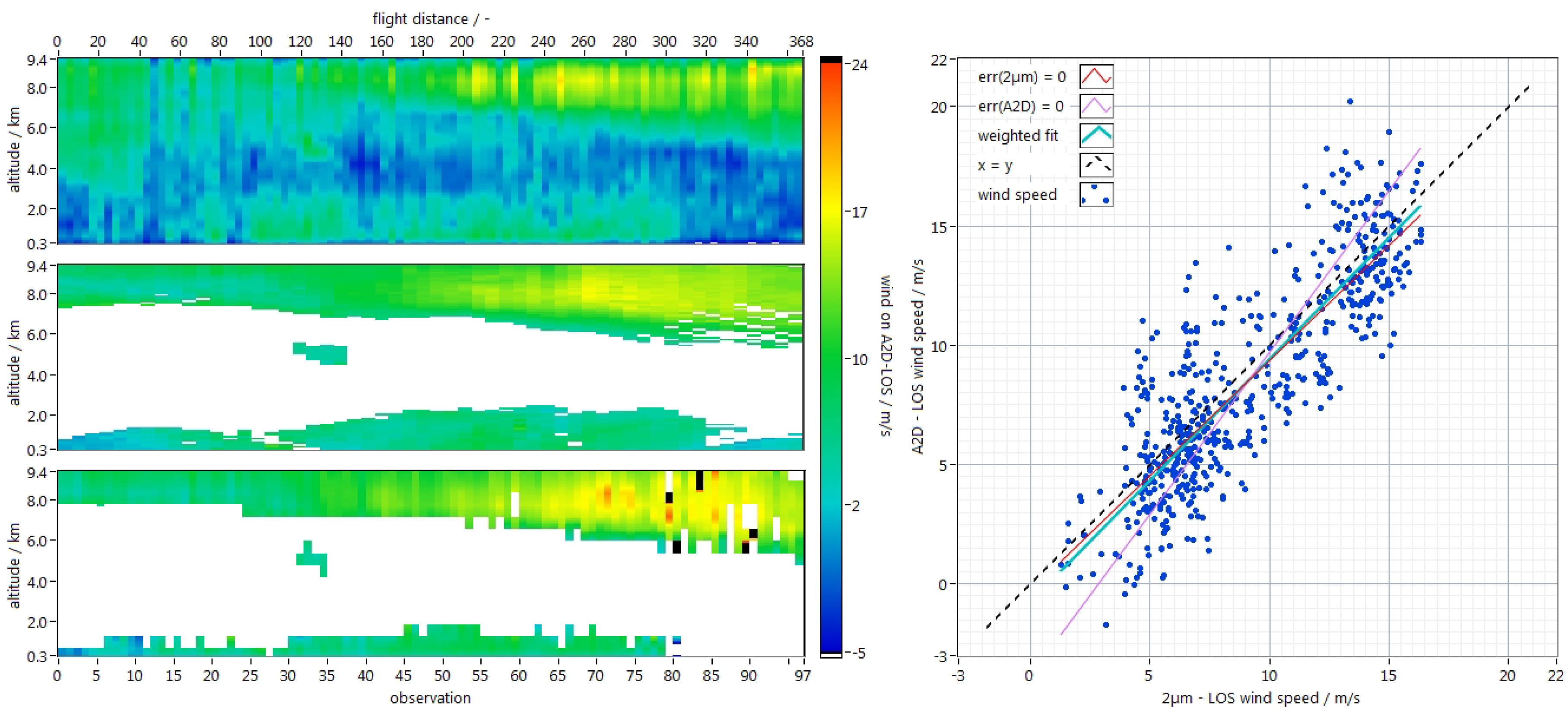Figure 11 exemplarily presents the A2D and 2-µm wind speeds derived from the backscatter signals (Figure 9) measured on 26 September 2009, (Marksteiner et al. [64] and Marksteiner [61]). By using its ability to perform conical scans, the 2-µm LiDAR determined three-dimensional wind vectors which had to be projected onto the A2D LOS. Very good agreement can be found in terms of wind field structure, gradients, minimum and maximum wind speed, and location of special features. LOS wind speeds of up to 24 m/s are detected by all three wind measurements in the upper right region, indicating a part of the jet stream. The small cloud mentioned regarding Figure 4 can be found at the same location in the A2D Mie and the 2-µm wind field. Also, the influence of the katabatic winds with their elevated aerosol load is visible in the middle of the scene between sea surface and 2 km. The way the winds obtained from the molecular backscatter close the gap in the wind field determined from the aerosol signal (bottom, white), perfectly shows the complementary nature of the Mie and Rayleigh channel of the A2D. Such a high coverage with wind measurements throughout the troposphere and lower stratosphere, only missing below optically thick clouds, justifies the increased effort in terms of calibration activities for a direct-detection LiDAR. However, the large amount of winds derived from molecular return comes at the expense of increased random errors compared to the 2-µm DWL.

A statistical comparison of A2D Rayleigh and 2-µm winds (Figure 11, right) including a linear fit reveals a slope of 1.02 (light blue bold line). Comparing A2D winds based on molecular return against 2-µm winds seems to be an odd approach when considering the effect of particulate backscatter from clouds or aerosols on the systematic error of the measured Rayleigh response (Dabas et al. [59]). However, the much higher sensitivity of the coherent 2-µm LiDAR with respect to particulate backscatter enables it to obtain wind measurements from regions with very low aerosol loads that are far from noticeably affecting the Rayleigh response. As an additional step of quality control, Rayleigh bins showing unusually high integration time-corrected and range-corrected intensities are invalidated according to Marksteiner [61]. We emphasize that we make use of a least squares straight-line fitting algorithm which allows for consideration of errors on both coordinates according to Press et al. [55]. Therefore, we estimated the general random errors of the 2-µm and the A2D winds to be 1 m/s and 2.5 m/s, respectively, (Marksteiner [61]), recently supported by the works of Chouza et al. [42] and Witschas et al. [16] assessing the performance of the 2-µm LiDAR. The faster and simpler approach typically applied to determine linear fits is to assume an error-free parameter on the x-axis.

Table 6. Intercepts and slopes of the linear fits through the scatterplots of the three selected wind measurement examples for three different allocations of wind speed random errors to the A2D and 2-µm system.

Date of Wind Scene	${\mathit{\sigma }}_{2\mathsf{\mu }\mathbf{m}}$ = 0 m/s	${\mathit{\sigma }}_{2\mathsf{\mu }\mathbf{m}}$ = 1.0 m/s & ${\mathit{\sigma }}_{\mathit{A}2\mathit{D}}$ = 2.5 m/s	${\mathit{\sigma }}_{\mathit{A}2\mathit{D}}$ = 0 m/s
	intercept/m/s
26.09.2009	−0.27	−0.76	−3.87
01.10.2009	1.39	1.46	1.80
25.05.2015	0.77	0.74	0.58
	slope
26.09.2009	0.97	1.02	1.36
01.10.2009	1.13	1.14	1.20
25.05.2015	1.00	1.00	1.04

summarizes the different slopes and intercepts resulting from linear fits through scatterplots for the three selected wind measurement scenes. It gives an impression of the implicitly accepted error (here in the assessment of the A2D performance) by assuming perfect wind measurements by the 2-µm LiDAR, which can amount up to 5% slope error as found for 26 September 2009. Generally, the slopes and intercepts derived from fit, including the errors on both coordinates, are much closer to the case of ${\sigma }_{2\mu m}$ = 0 m/s than to the more unrealistic case of ${\sigma }_{A2D}$ = 0 m/s. Except for Marksteiner [61], all slopes derived from such statistical comparison published in the past are based on the assumption that the 2-µm winds are error-free, i.e., they correspond to the left column of Table 6. Furthermore, the statistical comparison reveals a mean bias of −0.57 m/s, a correlation coefficient of 0.84, a standard deviation of 2.35 m/s and a mean absolute deviation of 2.13 m/s (

Table 7. Overview of the results of the statistical comparisons of A2D Mie and Rayleigh winds against 2-µm winds for the discussed cases (26 September 2009, 1 October 2009, 25 May 2015) and the complete data set from the 2015 campaign.

	2009/09/26	2009/10/01	2015/05/25	2015 Campaign	2015 Campaign
	(Rayleigh)	(Mie)	(Rayleigh)	(Rayleigh)	(Mie)
number of pairs	565	646	2212	12,647	1958
mean bias / m/s	−0.57	0.63	0.76	0.68	0.00
slope	1.02	1.14	1.00	1.00	1.01
correlation coeff. r	0.84	0.97	0.98	0.94	0.81
1.48 · MAD/m/s	2.13	1.30	1.77	2.08	2.32
standard dev./m/s	2.35	1.45	2.03	2.44	2.97

). A negative mean bias implies that on average the A2D winds are smaller than the 2-µm winds. The median absolute deviation (MAD) is defined as $median\left(\right|X_i-median\left(X\right)\left|\right)$ with $X_i$ being the differences between A2D and 2-µm winds. By multiplying the MAD with the factor of 1.48 (Huber [67]), it becomes a consistent estimator for the standard deviation in the case of a normal distribution. The MAD is given here as an additional parameter since the standard deviation is enhanced by the presence of outliers for a non-Gaussian distribution of the wind speed differences.

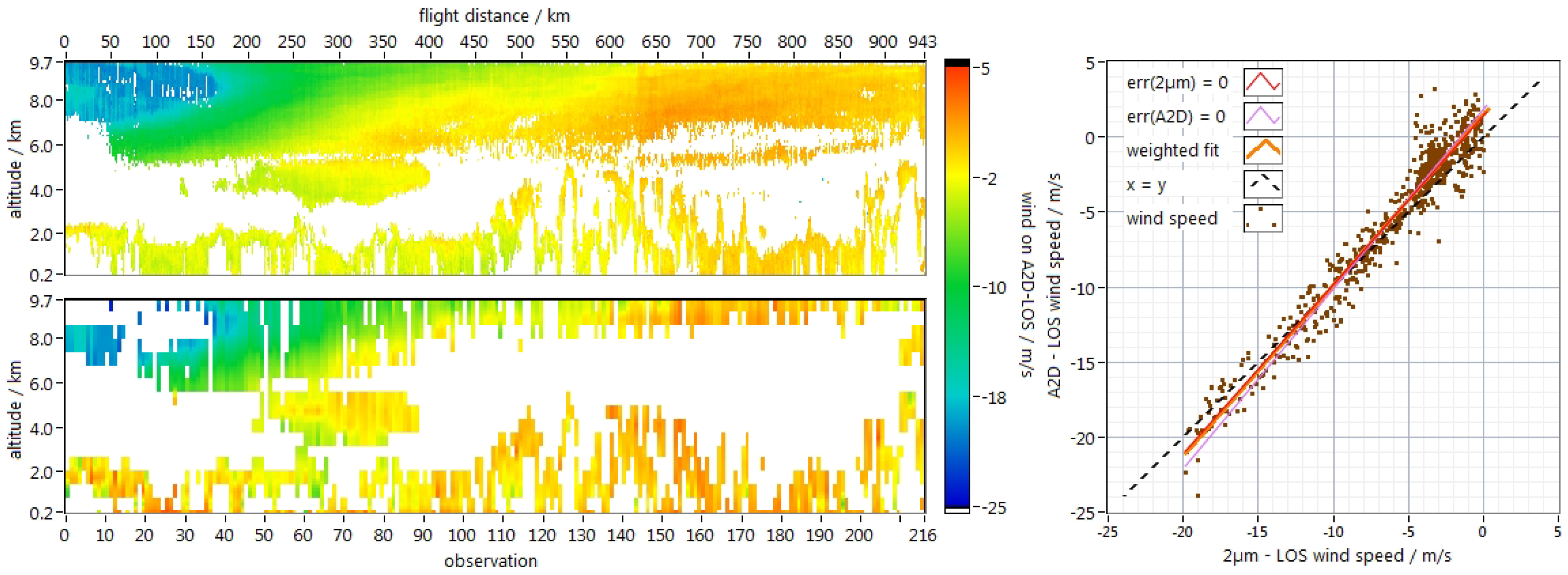
A comparison between 2-µm winds and A2D Mie winds for 1 October 2009, is presented in Figure 12. During this measurement period, the 2-µm LiDAR was operated with a fixed LOS, viewing in the same direction as the A2D, i.e., with an off-nadir angle of 20${}^{\circ }$. The flight leg stretched across the North Sea from the coast of Iceland to the coast of Norway (Figure 3, top). On the upper left, at the start of this scene, the jet stream with LOS wind speeds of up to −24 m/s was intersected. Here, the aerosol load was too low for a retrieval of valid A2D Mie winds but high enough for the 2-µm LiDAR. An impressive similarity between the two scenes is found in terms of the wind field structure. At altitudes between 3 km and 5 km and between observations 45 and 90, both LiDARs sensed a large optically thin cloud which the laser beams were able to penetrate, thus providing further wind measurements from a second cloud layer below. Optically thick broken clouds are distributed along the whole scene with varying cloud top height from less than 1 km (e.g., observation 25) up to 5 km (e.g., observation 125). The effect of a slight turn of the aircraft (white dashed arrow in Figure 3, top) by ≈15${}^{\circ }$ in heading angle is best visible as a small step in the wind speed measured by the 2-µm LiDAR at a flight distance of 625 km (Figure 12, top left). Considering 2-µm winds as the truth, higher LOS wind speeds (−10 m/s–0 m/s) are obviously underestimated by the A2D Mie channel (computed with calibration #2) whereas below −10 m/s the A2D Mie channel tended to measure higher (regarding the absolute value) wind speeds than the 2-µm LiDAR. One possible explanation is discussed by Sun et al. [68] who elucidate the performance of Aeolus in heterogeneous atmospheric conditions, i.e., in cases where atmospheric dynamics and optical properties vary strongly within the sampling volume.

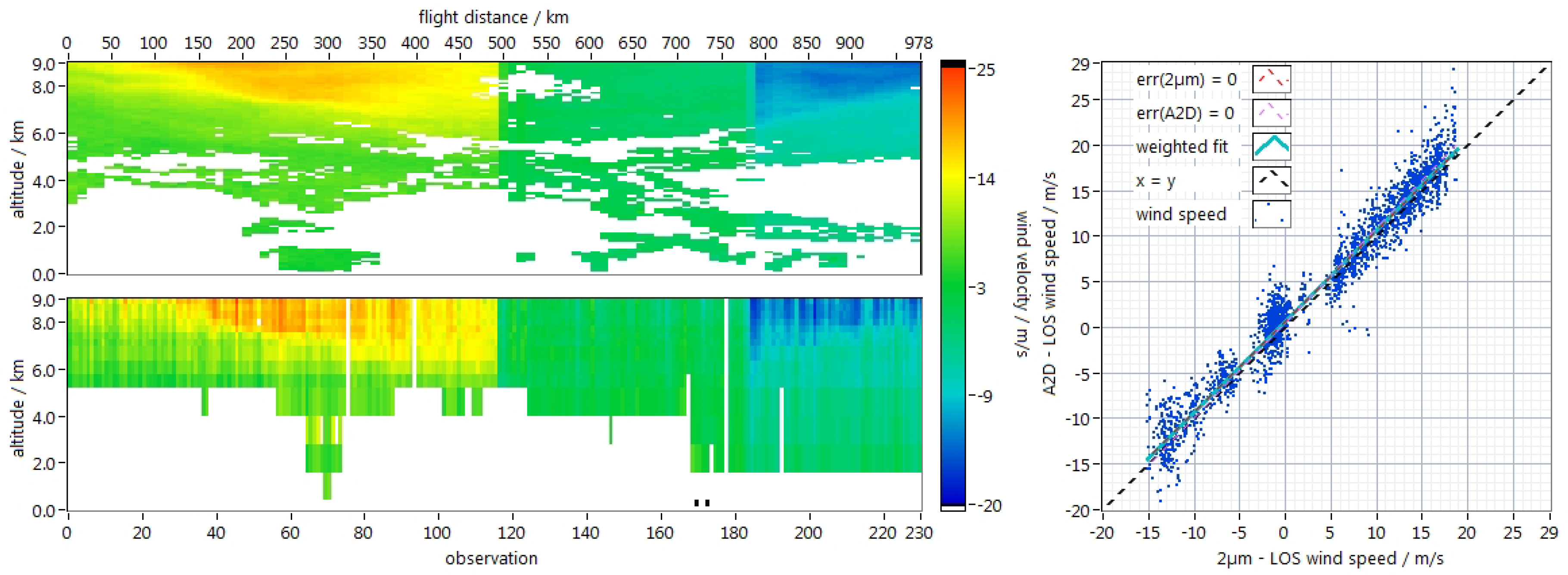
The longest A2D wind measurement scene with 88 min at a stretch was obtained on 25 May 2015 (Figure 13). In contrast to the two previous scenes above, this one comprises three flight legs of different length and with different aircraft heading directions. Aiming at detecting the jet stream, the flight track reached out half way towards Scotland initially in the southeasterly direction, before heading back towards Iceland in the opposite direction after two turns (Figure 3, right). These three segments are reflected in the three different wind field sections with the middle part located between observations 116 and 183 in Figure 13. With the A2D pointing to the right of the aircraft, strong positive (i.e., towards the instrument) LOS winds could be measured in the jet-stream region between 6 km and 9 km during the first segment. Accordingly, strong winds with negative sight were present for the third segment. The range of LOS wind speeds from −20 m/s up to 25 m/s is the largest measured by the A2D during a single flight. While flying against the jet stream in the middle segment, hence pointing perpendicularly to it, the A2D measured almost zero wind speed. No signal was obtained from below the optically thick clouds present at heights of around 5 km, particularly during the first and second segment. The measurements from within the clouds are biased due to contamination by strong Mie signal on the Rayleigh channel. Just as for Figure 11, only very low aerosol load and no clouds are present in this scene, which allows for a comparison of these two wind fields that are measured by different methods and based on different scattering mechanisms. Towards the end of the flight, from observation #170–#230, a large area without aerosol is present between 2 km and 5 km altitude where only the A2D Rayleigh channel was able to measure wind. The large range of wind speed strongly stabilizes the linear fit coefficients with respect to the different errors of the two LiDAR systems as can be seen exemplarily for the slope and intercept from Table 6.

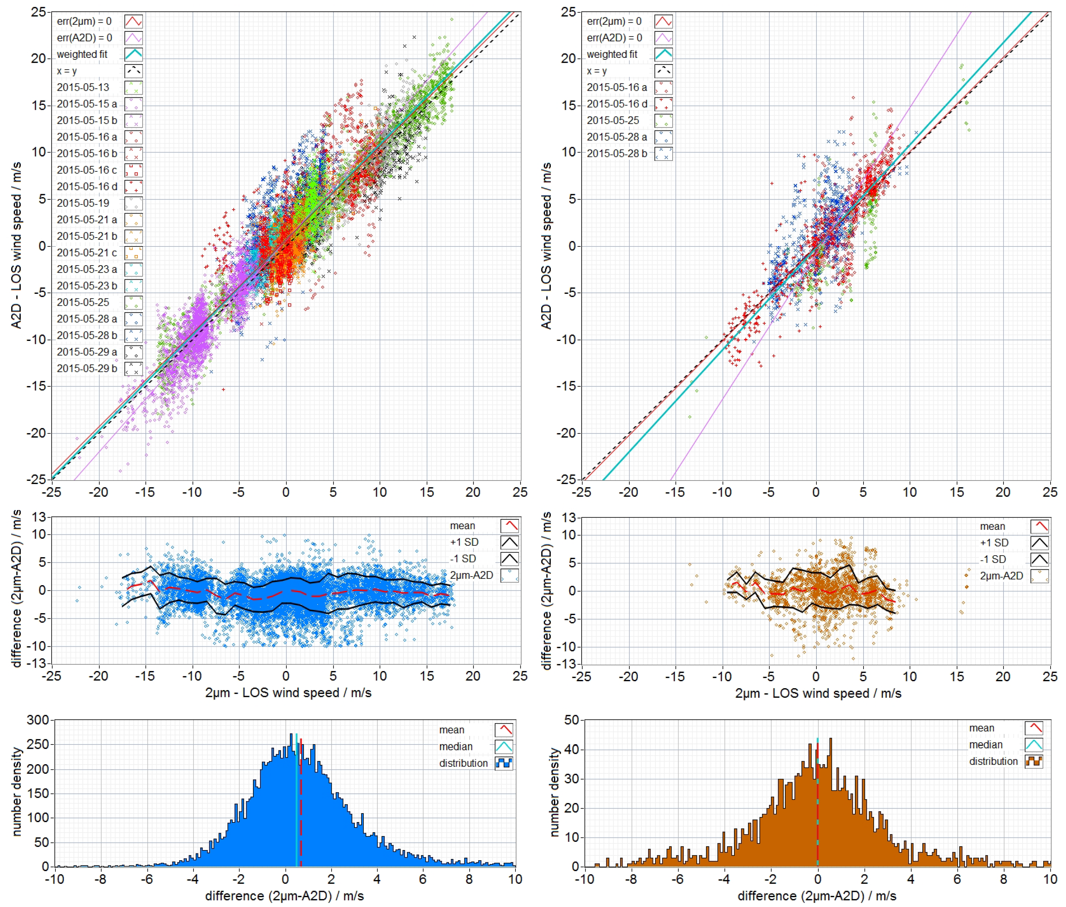
An overall statistical comparison of the winds derived from the A2D and the 2-µm LiDAR gives an estimation of the performance of the Mie and Rayleigh channel during the airborne campaign in 2015 (Figure 14). The sole usage of calibrations #3 and #7 for the Mie and Rayleigh channel, respectively, to process all these wind scenarios assures consistency in the statistical comparisons and essentially avoids additional errors that would be introduced by applying various calibrations (see Figure 8). Apart from a significantly larger number of bins entering the statistical comparison, the Rayleigh channel also enabled us to obtain a higher wind speed range than the Mie channel. Differences in wind speed between the A2D and the 2-µm LiDAR reach about ±12 m/s peak-to-peak for both the Mie and Rayleigh channel (Figure 14, middle) and show no clear wind speed-dependent bias. At the bottom, the probability density function of these differences is given. Regarding the Rayleigh channel, the distribution is slightly skewed as well as biased by 0.68 m/s (Table 7). The distribution for the Mie channel is broader, even including a small secondary maximum on its negative tail, thus, more clearly deviating from a Gaussian distribution which renders the allocated MAD the more credible figure compared to the standard deviation. Supported by many measurement scenes with rather small wind speed ranges, the seemingly vertical “striping” within the Rayleigh and Mie scatterplots at the top of Figure 14 indicates that the major contribution to the random error in these comparisons is induced by the A2D observations. Caused by very low aerosol content in the marine atmospheric boundary layer over the North Atlantic which additionally had been blocked several times by opaque cloud layers above, the Mie channel could provide only about a sixth of the bins entering the statistical comparison (1958) compared to the number of the Rayleigh channel (12,647). From this perspective, much more favorable conditions for Mie wind measurements could certainly be expected from flight in the tropics, during various desert dust events or volcanic eruptions. However, two more facts must be considered. On the one hand, we intentionally aimed at measuring in cloud-free conditions during both airborne campaigns to maximize the number of Rayleigh winds for a more reliable characterization of the Rayleigh channel. On the other hand, it is inherent to the Mie channel that in the case of optically thicker clouds, we usually receive a backscatter signal only from the uppermost one to three range-gates that overlap with the cloud.

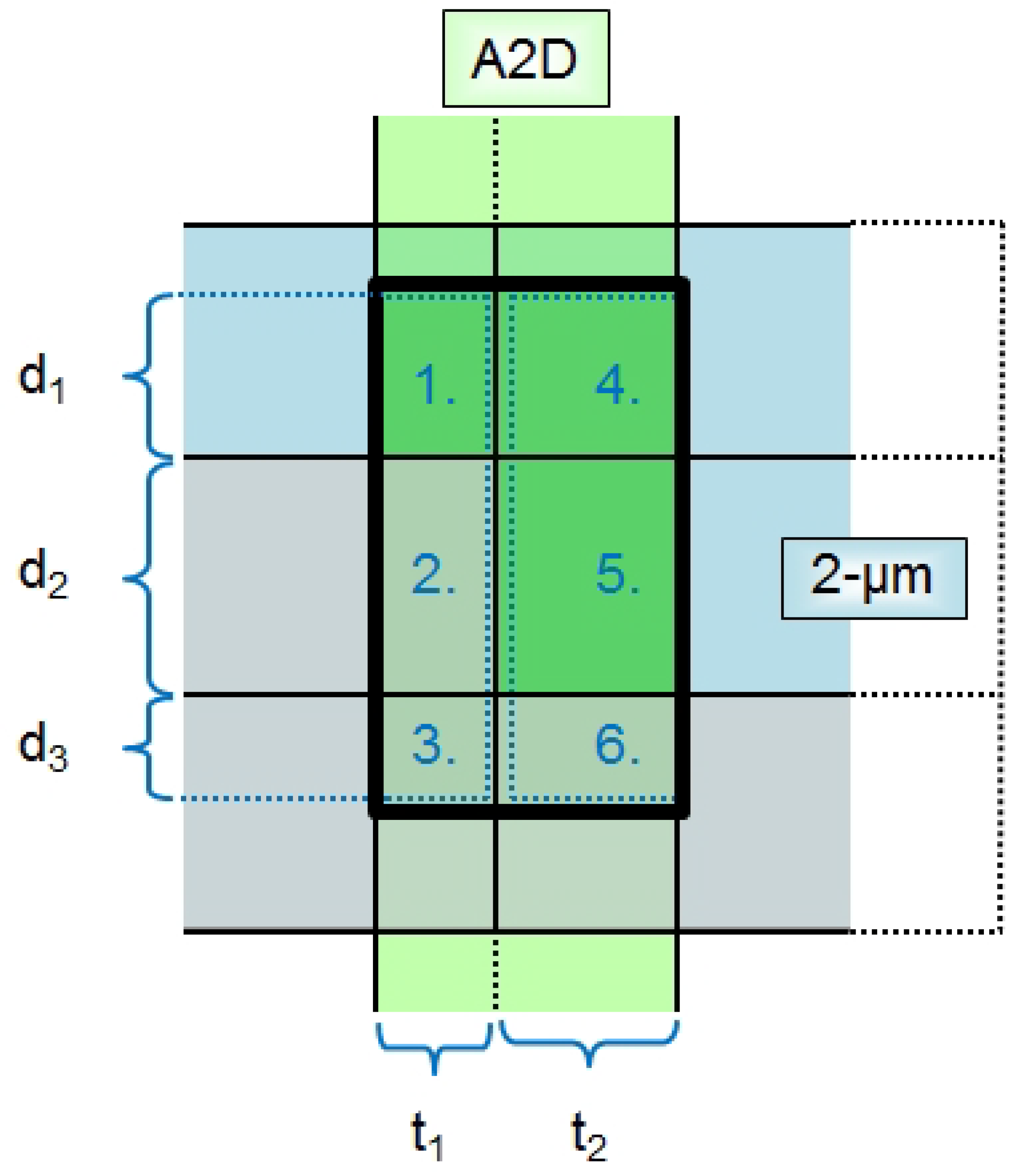
Finally, Table 7 summarizes the statistical parameters derived from the presented wind speed comparisons (Figure 11, Figure 12 and Figure 13). In addition to the number of compared wind speed bins (pairs), the mean bias, the slope, and the correlation coefficient, also given are the standard deviation and the MAD. For all statistical comparisons, we excluded the topmost three A2D range-gates from the wind scenes. Retrieved winds from that region are mainly biased due to the sensitivity of the interferometers to variations in the incidence angle. Regarding the coverage ratio for the A2D bins by valid 2-µm winds, we use a minimum threshold of 80% (Figure 10). Thereby, it is assured that wind observations which are input to the statistical comparison are not biased in the case of strong (particularly vertical) wind gradients. The significant positive linear relations between winds measured by the 2-µm LiDAR and the A2D are indicated by correlation coefficients of r > 0.81 and r > 0.94 for the Mie channel and the Rayleigh channel, respectively. As can be seen exemplarily for the Mie wind comparison for 1 October 2009, the slopes can deviate considerably from the ideal value of 1.0 for single flight sections due to the influence of small wind speed ranges in coaction with the allocation of random errors. Both the mean bias and standard deviation values given in Table 7, have to be seen in the context of the estimated performance of the 2-µm coherent detection LiDAR with a precision of <1 m/s and a bias of <0.3 m/s (Chouza et al. [42], Weissmann et al. [41], Witschas et al. [16]). It is emphasized that the statistics in Table 7 are subject to the results from the IRC comparison (Figure 8) that highlighted the delicate dependence of the final wind speeds on the IRC selected for wind retrieval. Statistical results regarding A2D wind observations obtained by Lux et al. [45] are similarly derived from single flights with a maximum of 352 wind pairs in the Rayleigh channel and 1246 pairs in the Mie channel. However, the analysis presented here is based on a significantly higher number of wind pairs for comparison (12,647 in the Rayleigh channel and 1958 in the Mie channel), thus providing increased confidence in the results.

8. Summary, Conclusions and Outlook

For the Aeolus satellite mission and its ALADIN instrument, an airborne demonstrator has been developed for the first time: the A2D. Its inherent similarities render the A2D a valuable tool supporting the pre-launch validation of Aeolus as well as the calibration/validation activities after launch in August 2018. We gave an overview of two airborne campaigns in the North Atlantic region in 2009 and 2015, when the direct-detection Doppler wind LiDAR A2D was operated along with a 2-µm heterodyne wind LiDAR measuring wind speed profiles in parallel from the same aircraft during more than 20 flights. We briefly introduced the different wind retrieval methods used by the A2D Rayleigh and Mie channel and broadly discussed the influence of the response calibrations on the accuracy of A2D wind observations. A new method to compare IRCs has been introduced and will be applied to Aeolus and A2D response calibrations in the future. Considering typically measured LOS wind speeds, an approximate uncertainty of 0.5 m/s–0.65 m/s must be allocated to the A2D Mie winds emanating from the uncertainty in the instrument response functions. Regarding the Rayleigh channel, this uncertainty is of the same order of magnitude, e.g., ≈0.7 m/s for low wind speeds at medium distances from the A2D instrument. The A2D has been providing highly accurate wind measurements continuously over the last decade. Exemplarily, statistical comparisons of A2D against 2-µm winds were presented for three selected wind measurement scenes from 2009 and 2015. The statistical parameters vary from flight to flight, depending, among other factors, on cloud structure, aerosol load and the stability of the instrument. The complete data set of the airborne campaign from 2015, comprising 12,647 wind observations in the Rayleigh channel and 1958 wind observations in the Mie channel, revealed random errors of ≈2.1 m/s and 2.3 m/s (MAD), respectively. Whereas a mean bias of 0.68 m/s was obtained for the Rayleigh channel, no bias was found for the Mie channel. A linear regression taking into account the allocation of different random errors for the A2D and the 2-µm wind speeds yielded slope errors of ≈1% for the Mie and less than 0.5% for the Rayleigh channel. The presented A2D wind observations validate the measurement principle of ESA’s Aeolus mission and verify its calibration approach. Future improvements mainly aim at correcting for the non-linearity error in the MRCs and improving the pointing stability of the A2D as well as the knowledge about it. With further dedicated airborne campaigns, both LiDARs, the A2D and the 2-µm, will participate in calibration/validation activities of the Aeolus mission after launch. A new laser transmitter operating at a 100 Hz repetition rate is currently under development for an upgraded A2D system. Improved stability of responses and wind speeds at the observational level are expected from recent successes in directing the Internal Reference signal through a fiber scrambler and therefore reducing speckle noise.

References

1. World Meteorological Organisation. Statements of Guidance for Global NWP, 2016. Available online: http://www.wmo.int/pages/prog/www/OSY/GOS-RRR.html (accessed on 1 May 2018).
2. Stoffelen, A.; Pailleux, J.; Källén, E.; Vaughan, J.M.; Isaksen, L.; Flamant, P.; Wergen, W.; Andersson, E.; Schyberg, H.; Culoma, A.; et al. The Atmospheric Dynamics Mission for global wind field measurement. Bull. Am. Meteorol. Soc. 2005, 86, 73–87. [Google Scholar] [CrossRef]
3. Baker, W.E.; Atlas, R.; Cardinali, C.; Clement, A.; Emmitt, G.D.; Gentry, B.M.; Hardesty, R.M.; Källen, E.; Kavaya, M.J.; Langland, R.; et al. Lidar-Measured Wind Profiles: The Missing Link in the Global Observing System. Bull. Am. Meteorol. Soc. 2014, 95, 543–564. [Google Scholar] [CrossRef]
4. Weissmann, M.; Cardinali, C. Impact of airborne Doppler lidar observations on ECMWF forecasts. Q. J. R. Meteorol. Soc. 2007, 133, 107–116. [Google Scholar] [CrossRef] [Green Version]
5. Marseille, G.J.; Stoffelen, A.; Barkmeijer, J. Impact assessment of prospective spaceborne Doppler wind lidar observation scenarios. Tellus A Dyn. Meteorol. Oceanogr. 2008, 60, 234–248. [Google Scholar] [CrossRef] [Green Version]
6. Horányi, A.; Cardinali, C.; Rennie, M.; Isaksen, L. The assimilation of horizontal line-of-sight wind information into the ECMWF data assimilation and forecasting system. Part I: The assessment of wind impact. Q. J. R. Meteorol. Soc. 2014, 141, 1223–1232. [Google Scholar] [CrossRef]
7. Stoffelen, A.; Marseille, G.J.; Bouttier, F.; Vasiljevic, D.; de Haan, S.; Cardinali, C. ADM-Aeolus Doppler wind lidar Observing System Simulation Experiment. Q. J. R. Meteorol. Soc. 2006, 132, 1927–1947. [Google Scholar] [CrossRef] [Green Version]
8. Marseille, G.J.; Stoffelen, A. Simulation of wind profiles from a space-borne Doppler wind lidar. Q. J. R. Meteorol. Soc. 2003, 129, 3079–3098. [Google Scholar] [CrossRef]
9. Tan, D.G.H.; Andersson, E. Simulation of the yield and accuracy of wind profile measurements from the Atmospheric Dynamics Mission (ADM-Aeolus). Q. J. R. Meteorol. Soc. 2005, 131, 1737–1757. [Google Scholar] [CrossRef] [Green Version]
10. Tan, D.G.H.; Andersson, E.; Fisher, M.; Isaksen, L. Observing-system impact assessment using a data assimilation ensemble technique: Application to the ADM—Aeolus wind profiling mission. Q. J. R. Meteorol. Soc. 2007, 133, 381–390. [Google Scholar] [CrossRef]
11. ESA. ADM-Aeolus Science Report; Technical Report SP-1311; European Space Agency: Paris, France, 2008. [Google Scholar]
12. Reitebuch, O. Atmospheric Physics: Background-Methods-Trends/Wind Lidar for Atmospheric Research; Schumann, U., Ed.; Springer: Berlin/Heidelberg, Germany, 2012; pp. 487–505. [Google Scholar]
13. Banakh, V.A.; Smalikho, I.N.; Rahm, S. Estimation of the refractive index structure characteristic of air from coherent Doppler wind lidar data. Opt. Lett. 2014, 39, 4321–4324. [Google Scholar] [CrossRef] [PubMed]
14. Shangguan, M.; Xia, H.; Wang, C.; Qiu, J.; Lin, S.; Dou, X.; Zhang, Q.; Pan, J.W. Dual-frequency Doppler lidar for wind detection with a superconducting nanowire single-photon detector. Opt. Lett. 2017, 42, 3541–3544. [Google Scholar] [CrossRef] [PubMed]
15. Koepp, F.; Rahm, S.; Smalikho, I. Characterization of Aircraft Wake Vortices by 2-μm Pulsed Doppler Lidar. J. Atmos. Ocean. Technol. 2004, 21, 194–206. [Google Scholar] [CrossRef]
16. Witschas, B.; Rahm, S.; Dörnbrack, A.; Wagner, J.; Rapp, M. Airborne Wind Lidar Measurements of Vertical and Horizontal Winds for the Investigation of Orographically Induced Gravity Waves. J. Atmos. Ocean. Technol. 2017, 34, 1371–1386. [Google Scholar] [CrossRef]
17. Dou, X.; Han, Y.; Sun, D.; Xia, H.; Shu, Z.; Zhao, R.; Shangguan, M.; Guo, J. Mobile Rayleigh Doppler lidar for wind and temperature measurements in the stratosphere and lower mesosphere. Opt. Express 2014, 22, A1203–A1221. [Google Scholar] [CrossRef] [PubMed]
18. Hildebrand, J.; Baumgarten, G.; Fiedler, J.; Hoppe, U.P.; Kaifler, B.; Lübken, F.J.; Williams, B.P. Combined wind measurements by two different lidar instruments in the Arctic middle atmosphere. Atmos. Meas. Tech. Discuss. 2012, 5, 4123–4156. [Google Scholar] [CrossRef]
19. Xia, H.; Dou, X.; Shangguan, M.; Zhao, R.; Sun, D.; Wang, C.; Qiu, J.; Shu, Z.; Xue, X.; Han, Y.; Han, Y. Stratospheric temperature measurement with scanning Fabry-Perot interferometer for wind retrieval from mobile Rayleigh Doppler lidar. Opt. Express 2014, 22, 21775–21789. [Google Scholar] [CrossRef] [PubMed]
20. Zhai, X.; Wu, S.; Liu, B.; Song, X.; Yin, J. Shipborne Wind Measurement and Motion-induced Error Correction of a Coherent Doppler Lidar over the Yellow Sea in 2014. Atmos. Meas. Tech. 2018, 11, 1313–1331. [Google Scholar] [CrossRef] [Green Version]
21. Hardesty, M.; Tucker, S.; Baidar, S.; Beubien, M. Airborne tests of an OAWL Doppler lidar: Results and potential for space deployment. In Proceedings of the 28th International Laser Radar Conference (ILRC 28), Bucarest, Romania, 25–30 June 2017; Volume 176, p. 02004. [Google Scholar]
22. Bruneau, D.; Blouzon, F.; Spatazza, J.; Montmessin, F.; Pelon, J.; Faure, B. Direct-detection wind lidar operating with a multimode laser. Appl. Opt. 2013, 52, 4941–4949. [Google Scholar] [CrossRef] [PubMed]
23. Schröder, T.; Lemmerz, C.; Reitebuch, O.; Wirth, M.; Wührer, C.; Treichel, R. Frequency jitter and spectral width of an injection-seeded Q-switched Nd:YAG laser for a Doppler wind lidar. Appl. Phys. B Lasers Opt. 2007, 87, 437–444. [Google Scholar] [CrossRef] [Green Version]
24. Li, T.; Fang, X.; Liu, W.; Gu, S.Y.; Dou, X. Narrowband sodium lidar for the measurements of mesopause region temperature and wind. Appl. Opt. 2012, 51, 5401–5411. [Google Scholar] [CrossRef] [PubMed]
25. Kavaya, M.J.; Beyon, J.Y.; Koch, G.J.; Petros, M.; Petzar, P.J.; Singh, U.N.; Trieu, B.C.; Yu, J. The Doppler Aerosol Wind (DAWN) Airborne, Wind-Profiling Coherent-Detection Lidar System: Overview and Preliminary Flight Results. J. Atmos. Ocean. Technol. 2014, 31, 826–842. [Google Scholar] [CrossRef]
26. Gentry, B.; Chen, H.; Cervantes, J.; Machan, R.; Reed, D.; Cargo, R.; Marx, C.; Jordan, P. Airborne Testing of the TWiLiTE Direct Detection Doppler Lidar. In Proceedings of the 16th Coherent Laser Radar Conference, Long Beach, CA, USA, 20–24 June 2011. [Google Scholar]
27. Herbst, J.; Vrancken, P. Design of a monolithic Michelson interferometer for fringe imaging in a near-field, UV, direct-detection Doppler wind lidar. Appl. Opt. 2016, 55, 6910–6929. [Google Scholar] [CrossRef] [PubMed]
28. Baumgarten, G. Doppler Rayleigh/Mie/Raman lidar for wind and temperature measurements in the middle atmosphere up to 80 km. Atmos. Meas. Tech. 2010, 3, 1509–1518. [Google Scholar] [CrossRef] [Green Version]
29. She, C.Y.; Yue, J.; Yan, Z.A.; Hair, J.W.; Guo, J.J.; Wu, S.H.; Liu, Z.S. Direct-detection Doppler wind measurements with a Cabannes-Mie lidar: A. Comparison between iodine vapor filter and Fabry-Perot interferometer methods. Appl. Opt. 2007, 46, 4434–4443. [Google Scholar] [CrossRef] [PubMed]
30. Reitebuch, O.; Lemmerz, C.; Nagel, E.; Paffrath, U.; Durand, Y.; Endemann, M.; Fabre, F.; Chaloupy, M. The Airborne Demonstrator for the Direct-Detection Doppler Wind Lidar ALADIN on ADM-Aeolus. Part I: Instrument Design and Comparison to Satellite Instrument. J. Atmos. Ocean. Technol. 2009, 26, 2501–2515. [Google Scholar] [CrossRef] [Green Version]
31. Tucker, S.C.; Weimer, C.S.; Baidar, S.; Hardesty, R.M. The Optical Autocovariance Wind Lidar. Part I: OAWL Instrument Development and Demonstration. J. Atmos. Ocean. Technol. 2018, 35, 2079–2097. [Google Scholar] [CrossRef]
32. Baidar, S.; Tucker, S.C.; Beaubien, M.; Hardesty, R.M. The Optical Autocovariance Wind Lidar. Part II: Green OAWL (GrOAWL) Airborne Performance and Validation. J. Atmos. Ocean. Technol. 2018, 35, 2099–2116. [Google Scholar] [CrossRef]
33. Ansmann, A.; Wandinger, U.; LeRille, O.; Lajas, D.; Straume, A.G. Particle backscatter and extinction profiling with the spaceborne high-spectral-resolution Doppler lidar ALADIN: methodology and simulations. Appl. Opt. 2007, 46, 6606–6622. [Google Scholar] [CrossRef] [PubMed]
34. Geiss, A.; Marksteiner, U.; Lux, O.; Lemmerz, C.; Reitebuch, O.; Kanitz, T.; Straume-Lindner, A.G. Retrieval of atmospheric backscatter and extinction profiles with the aladin airborne demonstrator (A2D). EPJ Web Conf. 2018, 176, 02021. [Google Scholar] [CrossRef] [Green Version]
35. Flamant, P.; Cuesta, J.; Denneulin, M.L.; Dabas, A.; Huber, D. ADM-Aeolus retrieval algorithms for aerosol and cloud products. Tellus A 2008, 60, 273–288. [Google Scholar] [CrossRef] [Green Version]
36. Reitebuch, O. Atmospheric Physics: Background-Methods-Trends/The Spaceborne Wind Lidar Mission ADM-Aeolus; Schumann, U., Ed.; Springer: Berlin/Heidelberg, Germany, 2012; pp. 815–826. [Google Scholar]
37. Durand, Y.; Chinal, E.; Endemann, M.; Meynart, R.; Reitebuch, O.; Treichel, R. ALADIN airborne demonstrator: A Doppler Wind lidar to prepare ESA’s ADM-Aeolus Explorer mission. In Proceedings of the SPIE (Earth Observing Systems XI), San Diego, CA, USA, 19–21 July 2006; Volume 6296, p. 62961D. [Google Scholar]
38. Reitebuch, O.; Endemann, M.; Engelbart, D.; Freudenthaler, V.; Lehmann, V.; Lemmerz, C.; Nagel, E.; Paffrath, U.; Rahm, S.; Witschas, B. Pre-Launch Validation of ADM-Aeolus with an airborne direct-detection wind lidar. In Proceedings of the 24th International Laser Radar Conference, Boulder, CO, USA, 23–27 June 2008; pp. 41–44. [Google Scholar]
39. Paffrath, U.; Lemmerz, C.; Reitebuch, O.; Witschas, B.; Nikolaus, I.; Freudenthaler, V. The Airborne Demonstrator for the Direct-Detection Doppler Wind Lidar ALADIN on ADM-Aeolus. Part II: Simulations and Rayleigh Receiver Radiometric Performance. J. Atmos. Ocean. Technol. 2009, 26, 2516–2530. [Google Scholar] [CrossRef] [Green Version]
40. Lemmerz, C.; Lux, O.; Reitebuch, O.; Witschas, B.; Wührer, C. Frequency and timing stability of an airborne injection-seeded Nd:YAG laser system for direct-detection wind lidar. Appl. Opt. 2017, 56, 9057–9068. [Google Scholar] [CrossRef] [PubMed]
41. Weissmann, M.; Busen, R.; Dörnbrack, A.; Rahm, S.; Reitebuch, O. Targeted Observations with an Airborne Wind Lidar. J. Atmos. Ocean. Technol. 2005, 22, 1706–1719. [Google Scholar] [CrossRef] [Green Version]
42. Chouza, F.; Reitebuch, O.; Jähn, M.; Rahm, S.; Weinzierl, B. Vertical wind retrieved by airborne lidar and analysis of island induced gravity waves in combination with numerical models and in situ particle measurements. Atmos. Chem. Phys. 2016, 16, 4675–4692. [Google Scholar] [CrossRef] [Green Version]
43. Chouza, F.; Reitebuch, O.; Benedetti, A.; Weinzierl, B. Saharan dust long-range transport across the Atlantic studied by an airborne Doppler wind lidar and the MACC model. Atmos. Chem. Phys. 2016, 16, 11581–11600. [Google Scholar] [CrossRef] [Green Version]
44. DuVivier, A.K.; Cassano, J.J.; Greco, S.; Emmitt, G.D. A Case Study of Observed and Modeled Barrier Flow in the Denmark Strait in May 2015. Mon. Weather Rev. 2017, 145, 2385–2404. [Google Scholar] [CrossRef]
45. Lux, O.; Lemmerz, C.; Weiler, F.; Marksteiner, U.; Witschas, B.; Rahm, S.; Schäfler, A.; Reitebuch, O. Airborne wind lidar observations over the North Atlantic in 2016 for the pre-launch validation of the satellite mission Aeolus. Atmos. Meas. Tech. 2018, 11, 3297–3322. [Google Scholar] [CrossRef] [Green Version]
46. Werner, C. Lidar: Range-Resolved Optical Remote Sensing of the Atmosphere/Doppler Wind Lidar; Weitkamp, C., Ed.; Springer Science+Business Media Inc.: Berlin, Germany, 2005; pp. 325–354. [Google Scholar]
47. Chanin, M.L.; Garnier, A.; Hauchecorne, A.; Porteneuve, J. A Doppler lidar for measuring winds in the middle atmosphere. Geophys. Res. Lett. 1989, 16, 1273–1276. [Google Scholar] [CrossRef]
48. Korb, C.L.; Gentry, B.M.; Li, S.X.; Flesia, C. Theory of the Double-Edge Technique for Doppler Lidar Wind Measurement. Appl. Opt. 1998, 37, 3097–3104. [Google Scholar] [CrossRef] [PubMed]
49. Flesia, C.; Korb, C.L. Theory of the Double-Edge Molecular Technique for Doppler Lidar Wind Measurement. Appl. Opt. 1999, 38, 432–440. [Google Scholar] [CrossRef] [PubMed]
50. Flesia, C.; Korb, C.L.; Hirt, C. Double-edge molecular measurement of lidar wind profiles at 355 nm. Opt. Lett. 2000, 25, 1466–1468. [Google Scholar] [CrossRef] [PubMed]
51. Gentry, B.M.; Chen, H.; Li, S.X. Wind measurements with 355-nm molecular Doppler lidar. Opt. Lett. 2000, 25, 1231–1233. [Google Scholar] [CrossRef] [PubMed]
52. Witschas, B.; Lemmerz, C.; Reitebuch, O. Horizontal lidar measurements for the proof of spontaneous Rayleigh-Brillouin scattering in the atmosphere. Appl. Opt. 2012, 51, 6207–6219. [Google Scholar] [CrossRef] [PubMed]
53. Garnier, A.; Chanin, M.L. Description of a Doppler Rayleigh lidar for measuring winds in the middle atmosphere. Appl. Phys. B Lasers Opt. 1992, 55, 35–40. [Google Scholar] [CrossRef]
54. Nelder, J.A.; Mead, R. A Simplex Method for Function Minimization. Comput. J. 1965, 7, 308–313. [Google Scholar] [CrossRef]
55. Press, W.H.; Vetterling, W.T.; Teucholsky, S.A.; Flannery, B.P. Numerical Recipies in C—The Art of Scientific Computing; Cambridge University Press: Cambridge, UK, 1992. [Google Scholar]
56. Weiler, F. Bias Corretion Using Ground Echoes for the Airborne Demonstrator of the Wind Lidar on the ADM-Aeolus Mission. Master’s Thesis, University of Innsbruck, Innsbruck, Austria, 2017. [Google Scholar]
57. Horányi, A.; Cardinali, C.; Rennie, M.; Isaksen, L. The assimilation of horizontal line-of-sight wind information into the ECMWF data assimilation and forecasting system. Part II: The impact of degraded wind observations. Q. J. R. Meteorol. Soc. 2015, 141, 1233–1243. [Google Scholar] [CrossRef]
58. Witschas, B.; Lemmerz, C.; Reitebuch, O. Daytime measurements of atmospheric temperature profiles (2–15 km) by lidar utilizing Rayleigh-Brillouin scattering. Opt. Lett. 2014, 39, 1972–1975. [Google Scholar] [CrossRef] [PubMed]
59. Dabas, A.; Denneulin, M.L.; Flamant, P.; Loth, C.; Garnier, A.; Dolfi-Bouteyre, A. Correcting winds measured with a Rayleigh Doppler lidar from pressure and temperature effects. Tellus A 2008, 60, 206–215. [Google Scholar] [CrossRef] [Green Version]
60. Tan, D.G.H.; Andersson, E.; de Kloe, J.; Marseille, G.J.; Stoffelen, A.; Poli, P.; Denneulin, M.L.; Dabas, A.; Huber, D.; Reitebuch, O.; et al. The ADM-Aeolus wind retrieval algorithms. Tellus A 2008, 60, 191–205. [Google Scholar] [CrossRef] [Green Version]
61. Marksteiner, U. Airborne Wind Lidar Observations for the Validation of the ADM-Aeolus Instrument. Ph.D. Thesis, Technische Universität München, Munich, Germany, 2013. [Google Scholar]
62. Witschas, B.; Marksteiner, U.; Reitebuch, O.; Lemmerz, C.; Lux, O. Analysis of Enhanced Noise in A2D Observations; Final Report; European Space Agency (ESA): Paris, France, 2016. [Google Scholar]
63. Reitebuch, O.; Huber, D.; Leike, I. ADM-Aeolus Algorithm Theoretical Basis Document ATBD Level1B Products; Final Report; European Space Agency (ESA): Paris, France, 2018. [Google Scholar]
64. Marksteiner, U.; Reitebuch, O.; Rahm, S.; Nikolaus, I.; Lemmerz, C.; Witschas, B. Airborne direct-detection and coherent wind lidar measurements along the east coast of Greenland in 2009 supporting ESA’s Aeolus mission. In Proceedings of the SPIE Conference on Lidar Technologies, Techniques, and Measurements for Atmospheric Remote Sensing VII, Prague, Czech Republic, 19–22 September2011; p. 81820J. [Google Scholar]
65. Marksteiner, U.; Reitebuch, O.; Lemmerz, C.; Lux, O.; Rahm, S.; Witschas, B.; Schäfler, A.; Emmitt, D.; Greco, S.; Kavaya, M.J.; et al. Airborne direct-detection and coherent wind lidar measurements over the North Atlantic in 2015 supporting ESA’s aeolus mission. In Proceedings of the 28th International Laser Radar Conference (ILRC 28), Bucarest, Romania, 25–30 June 2018; Volume 176, p. 02011. [Google Scholar]
66. Reitebuch, O.; Marksteiner, U.; Lemmerz, C. WindVal–Joint DLR-ESA-NASA Wind Validation for Aeolus; Final Report; European Space Agency (ESA): Paris, France, 2017. [Google Scholar]
67. Huber, P.J. Robust Statistics; John Wiley & Sons, Inc.: Hoboken, NJ, USA, 1981. [Google Scholar]
68. Sun, X.J.; Zhang, R.W.; Marseille, G.J.; Stoffelen, A.; Donovan, D.; Liu, L.; Zhao, J. The performance of Aeolus in heterogeneous atmospheric conditions using high-resolution radiosonde data. Atmos. Meas. Tech. 2014, 7, 2695–2717. [Google Scholar] [CrossRef] [Green Version]
Figure 1. Modelled spectra of the emitted laser pulse (violet), the molecular backscatter (light blue) from the atmosphere (Rayleigh Brillouin lineshape) and the transmitted intensities (green and pink areas) through the respective filters A (red line) and B (green line) of the Rayleigh spectrometer. The dotted lines represent the associated response curves R R for the broadband molecular return (dark blue) and the narrow-band laser spectrum (black circles) in steps of 50 MHz. The two vertical black dashed lines span a typical calibration range of 1.5 GHz around the crosspoint of the two filter transmissivity curves.
Remotesensing 10 02056 g001
Figure 2. Left: The emitted laser pulse (bold arrows) is directed towards the atmosphere, the wavelength meter and the spectrometers for Internal Reference measurements (LPO: low power oscillator, PLL: phase locked loop, SHG: second harmonic generation, THG: third harmonic generation, RLH: Reference Laser Head). The received backscatter signal is transmitted through the Front Optics and then analyzed by two different spectrometers. A small fraction of the backscatter signal is guided towards a UV-camera for co-alignment purposes (thin dashed arrow). ACCDs detect the incoming photons and analogue digital converters (ADC) translate the signal. Right: Simplified operation principle of the ACCDs used for the Mie and Rayleigh channel. After acquisition in the imaging zone, the signal is shifted to the memory zone via a transfer row. From there, the charges are pushed to the read-out register and finally to the ADC. Signal levels are color-coded from black (no signal) and blue (low) to red (high).
Remotesensing 10 02056 g002
Figure 3. Flight tracks of the DLR Falcon during the airborne campaigns 2009 (top) and 2015 (bottom). Solid and dashed arrows indicate the locations of calibrations and wind measurements discussed here. The inset shows a zoom into the region of calibration #1 (orange) and #2 (blue) with black arrows marking the start and direction of the respective tracks. (background image: ©2018 Google Earth).
Remotesensing 10 02056 g003
Figure 4. Summed intensities of the Rayleigh (top) and the Mie channel (bottom) for each range-gate during calibration #7 performed on 23 May 2015. The first observation started at 18:49.41 UTC, the last at 19:12.29 UTC. For the actual analysis of this Rayleigh and Mie response calibration, only the observations #9–#69 respectively #17 - #61 (both included in each case) are considered, marked by grey boxes. Range-gate #5 and range-gates #20–#23 have the same vertical thickness of 315 m, whereas it is 630 m for range-gates #6–#19. The Internal Reference signal is shown in range-gate #4, corresponding to a flight altitude of 10.1 km. The relative frequency is given with respect to the Rayleigh crosspoint of the Internal Reference which coincides here with the Mie center frequency, i.e., a Mie response of 7.5 pixel.
Remotesensing 10 02056 g004
Figure 5. Instrument response functions of seven airborne calibrations in 2009 and 2015 for the Mie channel Internal Reference (a) and ground return (b) as well as the Rayleigh channel Internal Reference (c) and atmospheric return (d). Frequencies were measured by the wavemeter and are given here with respect to the Mie center and the Rayleigh filter crosspoint, respectively.
Remotesensing 10 02056 g005
Figure 6. Top: Non-linearities (dashed) and polynomial fits of 5th-order (solid, bold) for the Rayleigh atmospheric response functions of all seven airborne calibrations. The straight section between −300 MHz to −100 MHz of IRC #6 bridges several frequency steps that had to be excluded owing to a temporal outage of the A2D co-alignment control loop. Bottom: Non-linearities of the Internal Reference in the Mie channel.
Remotesensing 10 02056 g006
Figure 7. Residual error (in units of response) around polynomial fits through the measured Rayleigh response calibration curves per range-gate and calibration. Starting from a distance of 6 km, the calibrations #1–#5 are affected by the ground return signal of the Greenland ice shield and are completely blocked below the ground.
Remotesensing 10 02056 g007
Figure 8. Average differences in wind speed for two randomly selected instrument response calibrations for atmospheric range-gates at different distances in the Rayleigh channel (left) and for the ground return in the Mie channel (right). Only calibrations from 2015 are considered here. Additionally, calibration #6 is excluded for the Rayleigh channel owing to a temporal outage of the co-alignment control loop.
Remotesensing 10 02056 g008
Figure 9. DCO and background corrected intensities of the Rayleigh channel (top) and Mie channel (bottom) for the flight from 26 September 2009, between 11:50.06 and 12:19.08 UTC. Range-gate #4 corresponds to the Internal Reference. The first atmospheric range-gates show a strong backscatter signal from the near field. Range-gates #6 to #23 have the same vertical thickness of 592 m. Increased intensities in range-gate #22 (and partly #21) represent the backscatter from the sea surface. Cloud backscatter is visible between observation 30 and 35 in range-gates #13 and #14.
Remotesensing 10 02056 g009
Figure 10. Method to compare A2D winds (green) with winds measured by the 2-µm reference LiDAR (blue). Grey color symbolizes invalid 2-µm winds. The bold black rectangle envelopes a single A2D observation which is covered by six 2-µm wind measurement bins, proportionately different on vertical (d 1 –d 3 ) and horizontal, i.e., temporal, scale (t 1 , t 2 ).
Remotesensing 10 02056 g010
Figure 11. Left: A2D Rayleigh (top) and Mie LOS wind speeds (bottom) as well as 2-µm winds (middle) for the flight section from 26 September 2009 between 11:50.06 and 12:19.08 UTC. The A2D winds are interpolated onto a vertical grid of 100 m resolution. White and black colors represent invalid winds due to a low aerosol signal. Both the A2D Rayleigh and Mie winds are computed using calibration #2 from 21 September 2009. Right: The statistical comparison between A2D Rayleigh and 2-µm winds. The blue line corresponds to a fit attributing 1 m/s and 2.5 m/s random error to the 2-µm and A2D DWL, respectively. Equivalently, the red and magenta line correspond to cases which assume perfect 2-µm and A2D wind measurements, respectively.
Remotesensing 10 02056 g011
Figure 12. Left: LOS wind measurements by the 2-µm LiDAR (top) and the A2D Mie channel (bottom) based on aerosol and cloud backscatter obtained on 1 October 2009, between 09:35.02 and 10:39.45 UTC. The A2D winds are interpolated onto a vertical grid of 100 m resolution (left). White color represents invalid winds due to low signal. The A2D Mie winds are computed using calibration #2 from 21 September in 2009. Right: The statistical comparison in which the orange line corresponds to a fit attributing 1 m/s and 2.5 m/s random error to the 2-µm and A2D DWL, respectively. Equivalently, the red and magenta line correspond to cases which assume perfect 2-µm and A2D wind measurements, respectively.
Remotesensing 10 02056 g012
Figure 13. Left: Wind measurements by the 2-µm LiDAR (top) and the A2D Rayleigh channel (bottom) obtained on 25 May 2015, between 15:24.03 and 16:47.44 UTC. The Rayleigh winds are interpolated onto a vertical grid of 100 m resolution. White color represents invalid winds due to no or contaminated signal. The Rayleigh winds are computed using calibration #7 from 23 May in 2015. Right: The statistical comparison in which the blue line corresponds to a fit attributing 1 m/s and 2.5 m/s random error to the 2-µm and A2D DWL, respectively. Equivalently, the dashed red and magenta line, lying almost on top of the blue line, correspond to cases which assume perfect 2-µm and A2D wind measurements, respectively.
Remotesensing 10 02056 g013
Figure 14. Overall statistical comparisons for the Rayleigh channel (left) and the Mie channel winds (right) derived from the entire flight campaign in 2015. Presented are the wind measurements by the 2-µm LiDAR compared to A2D winds (top) for different days (color-coded). The bold blue lines correspond to a fit attributing 1 m/s and 2.5 m/s random error to the 2-µm and A2D DWL, respectively. Equivalently, the red and magenta lines correspond to cases which assume perfect 2-µm and A2D wind measurements, respectively. The differences in wind speed (A2D - 2-µm ) between both LiDARs (center) are shown together with the mean value (red dashed lines) and ±1 standard deviation (black lines). The probability density functions of these differences (bottom) are given along with the mean (dashed red line) and median value (blue line).
Remotesensing 10 02056 g014