Annual Cropland Mapping Using Reference Landsat Time Series—A Case Study in Central Asia


1
Key Laboratory of Agricultural Remote Sensing, Ministry of Agriculture, Institute of Agricultural Resources and Regional Planning, Chinese Academy of Agricultural Sciences, Beijing 100081, China
2
MapTailor Geospatial Consulting, 53113 Bonn, Germany
3
International Centre for Agricultural Research in Dry Areas (ICARDA), Cairo 11431, Egypt
*
Authors to whom correspondence should be addressed.
Remote Sens. 2018, 10(12), 2057; https://0-doi-org.brum.beds.ac.uk/10.3390/rs10122057
Submission received: 19 November 2018
/
Revised: 5 December 2018
/
Accepted: 11 December 2018
/
Published: 18 December 2018
(This article belongs to the Special Issue Monitoring Agricultural Land-Use Change and Land-Use Intensity)
Abstract
:Mapping the spatial and temporal dynamics of cropland is an important prerequisite for regular crop condition monitoring, management of land and water resources, or tracing and understanding the environmental impacts of agriculture. Analyzing archives of satellite earth observations is a proven means to accurately identify and map croplands. However, existing maps of the annual cropland extent either have a low spatial resolution (e.g., 250–1000 m from Advanced Very High Resolution Radiometer (AVHRR) to Moderate-resolution Imaging Spectroradiometer (MODIS); and existing high-resolution maps (such as 30 m from Landsat) are not provided frequently (for example, on a regular, annual basis) because of the lack of in situ reference data, irregular timing of the Landsat and Sentinel-2 image time series, the huge amount of data for processing, and the need to have a regionally or globally consistent methodology. Against this backdrop, we propose a reference time-series-based mapping method (RBM), and create binary cropland vs. non-cropland maps using irregular Landsat time series and RBM. As a test case, we created and evaluated annual cropland maps at 30 m in seven distinct agricultural landscapes in Xinjiang, China, and the Aral Sea Basin. The results revealed that RBM could accurately identify cropland annually, with producer’s accuracies (PA) and user’s accuracies (UA) higher than 85% between 2006 and 2016. In addition, cropland maps by RBM were significantly more accurate than the two existing products, namely GlobaLand30 and Finer Resolution Observation and Monitoring of Global Land Cover (FROM–GLC).
1. Introduction
Understanding the spatial and temporal dynamics of cropland is an important prerequisite for regular monitoring of agricultural production (crop area and productivity), supporting management of land and water resources, or tracing and understanding environmental impacts of agriculture [1,2]. Dependable spatial information is required for analyzing land use intensity or agricultural land abandonment [3]. The challenge is that in many regions, agricultural statistics are outdated, of doubtful quality [4], or missing adequate sub-national historical inventory data [5]. One such region is Central Asia, which has experienced unprecedented expansion of agricultural production, widespread cropland degradation, and abandonment [6,7]. The expansion and inefficient management have resulted in a permanent net loss of freshwater resources during the last three decades [8,9]. Due to aridity and a growing population, there is growing risk of potential conflicts over shared but sparse water resources [10].
The literature on cropland mapping with satellite remote sensing is replete with various approaches and types of data used for this purpose. For example, previous studies used multi-temporal images of the moderate-resolution imaging spectroradiometer (MODIS) sensors on board the Terra and Aqua satellites with a 500 m pixel size to create a spatial distribution of cropland annually [11]. The GlobCover data set from the European Space Agency (ESA, Paris, France) was created from the medium resolution imaging spectrometer (MERIS) with a 300 m pixel size [12]. Whilst the previous examples highlight studies that created annual cropland maps that allow for a monitoring application, their relatively coarse resolution can hamper local and field-level studies. Using higher spatial resolution data, such as those from Landsat (30 m) that range back for decades, provides the data basis for many high resolution data sets [13], including global products such as the Finer Resolution Observation and Monitoring of Global Land Cover (FROM–GLC) [14], Globaland30 [15], or the Global Food Security Support Analysis Data (GFSAD30AFCE) [16]. However, 30 m cropland maps at global scale are provided at certain years, such as 2000, 2010 and 2015, so annual cropland maps cannot be generated.
One potentially limiting factor is that the image time series acquired by the Landsat system contain gaps due to low revisit frequency (16-day) and cloud cover [17], or missing ground stations. Several strategies have been devised to cope with the limited availability of calibration data and satellite data heterogeneity (such as irregular Landsat time series). For example, gap filling and data fusion techniques were proposed to generate image series at 30-m resolution with a high and regular temporal frequency [18,19,20]. Liu, et al. [21] generated land cover products with five-year intervals in China at 30 m, but these methods are time-consuming and labor-intensive from a computational point of view.
Furthermore, the availability of in situ data is key to calibrating supervised classifiers. However, collecting this information is time-consuming and can become prohibitively expensive, and human interpretation of spectral signatures from satellite images can be resource-intensive, time-consuming, and difficult to repeat over space and time [22]. Some methods seek to identify cropland extent without the use of any ground training samples [13]. Yan and Roy [23] proposed an automatic object-based approach to identify crop fields at 30 m resolution; the method showed good potential to identify crop fields with clearly boundaries from 30-m resolution images. An alternative strategy is generating time series by calculating phenological characteristics (metrics) from vegetation index time series and classifying knowledge-based temporal features [22,24,25,26,27]. However, one potential drawback of this method is that the thresholds may induce uncertainty in the labeling process.
Given the above discussion, we present a procedure named reference time-series-based mapping method (RBM), that can be applied to different agricultural landscapes (i.e., different crop types or use intensities) for annual cropland mapping. It consists of creating reference time series from training samples and regular Landsat time series in certain years with artificial immune networks (AINs). Then, the reference time series are used to process irregular Landsat data to generate annual cropland maps at 30 m resolution. The proposed methodology was applied to seven distinct agricultural landscapes in Central Asia (Aral Sea Basin and Xinjiang). We evaluated the annual crop maps using independent test data and by comparing them with existing 30 m-cropland products.
2. Study Area
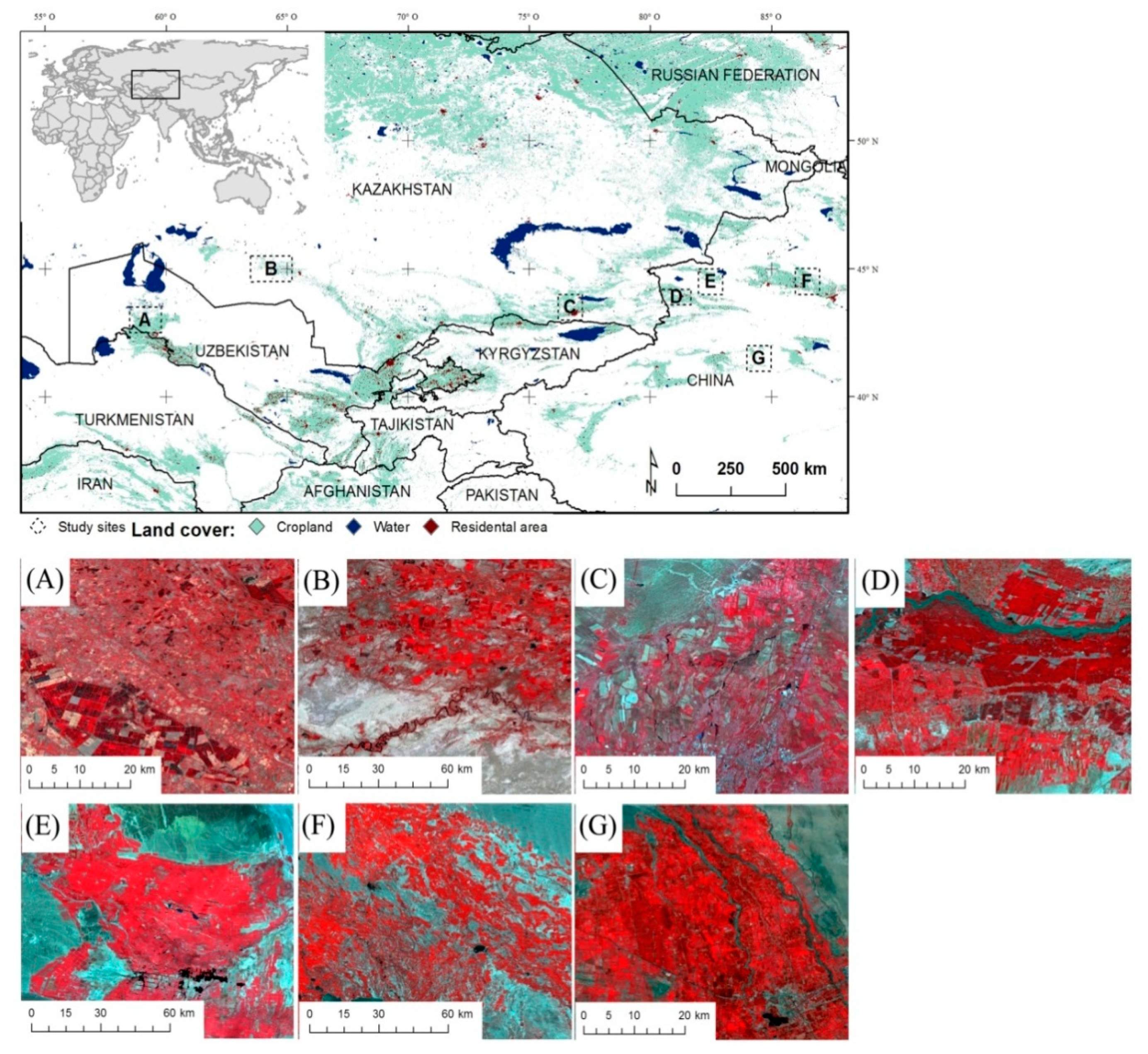
The study area consists of seven distinct agricultural landscapes in Central Asia. The choice of these sites was oriented towards having a range of different landscapes in terms of cropping pattern, crop rotation, crop types, biophysical conditions (e.g., soil types), irrigation infrastructure, and irrigation management.
Four sites were selected in Xinjiang, which partly encompasses the Ili-Balkash basin, and three were selected in the Aral Sea basin (Figure 1). Both regions are located in Central Asia at the heart of the Eurasian landmass. The Aral Sea basin covers parts of post-Soviet Central Asia and encompasses circa 1.7 million km2. Under Soviet leadership, the Aral Sea basin experienced a pronounced increase in irrigated cropland area, from 5.4 million hectares (mha) (1950s) to around 8 mha (1990s) [28]. However, the unsustainable withdrawal of freshwater and inefficient water use reduced the inflow of rivers. As a result, the Aral Sea dried out almost completely, and the irrigated cropland became largely salinized and partly abandoned [28]. After the disintegration of the Soviet Union and the subsequent institutional and economic changes, agricultural production decreased sharply in many regions of the Aral Sea basin [29]. In Xinjiang, China, irrigated cropland significantly expanded from 6.68 mha (2000) to 8.46 mha (2010) [30,31], mainly in traditional oasis areas, such as the south and north foothills of the Tianshan Mountains [32,33]. China’s national development strategy in western areas and improved techniques for conserving water led to fast cropland expansion in Xinjiang [34,35]. The seven study areas are located in three countries with arid continental and dry climates, and contain representative crop types of Central Asia and crop fields of different sizes. Precipitation is in a range of circa 100–250 mm per year, and agriculture in all study areas relies on irrigation [36]. The Bole (BL; E in Figure 1) and Manas (MNS; F in Figure 1) landscapes are located in the northern part of Xinjiang, China. The major crop type, i.e., the crop that covers most of the cultivated area in these two study sites, is cotton (Table 1), and the cropland is homogenously shaped with a relatively large field size. The third site is situated in Luntai county (LT; G in Figure 1) in southern Xinjiang, where the agricultural landscapes are more fragmented. Major crops in this region are cotton, wheat, and maize. The fourth study region is located in Yining city (YN; D in Figure 1) of Xinjiang; the major crops in this region are cotton and wheat. Karakalpakstan (KKP; A in Figure 1) and Kyzl-Orda (KYZ; B in Figure 1) are located in the Aral Sea basin and characterized by vast, regularly shaped agricultural systems with only a few predominating crops (rice and alfalfa in KYZ, winter wheat and cotton in KKP) [6]. Almaty (ALM; C in Figure 1) is located in the southeast of Kazakhstan. The major crops cultivated there are wheat, barley, and cotton.
3. Data Sets
3.1. Satellite Data
We sourced all available Landsat-5, -7, and -8 images falling into the area of interest between April and October (this period was defined as a growing period) during the observation period from 2001 to 2016. The Landsat images used in this study were Tier 1 surface reflectance (SR) data, which are available from the Google Earth platform.
3.2. Existing Global Land Cover Maps
There are two existing global-scale land-cover products containing cropland extent that can be used to compare with the cropland maps generated in this study. The first layer, the Finer Resolution Observation and Monitoring of Global Land Cover (FROM–GLC), is a 30-m global land cover product from 2010. To generate the product, 91,433 training samples and 38,664 test samples were collected by visual interpretation of TM/ETM+ images. A segmentation approach was then used to integrate multi-resolution datasets, including Landsat TM/ETM+, MODIS Enhanced Vegetation Index (EVI) time series, bioclimatic variables, Digital Elevation Model DEMs, and soil–water variables, and the random forest (RF) classifier was used to classify land cover type. Finally, two coarse resolution impervious maps were used to mask the residential regions. FROM–GLC had an overall accuracy of 65.51%, and producer’s and user’s accuracies for cropland were 66.62% and 57.60%, respectively [14,37].
The second layer, GlobeLand30, is another global land-cover dataset with a 30-m spatial resolution. It contains 10 land cover classes: cropland, forest, grassland, shrubland, wetland, water bodies, tundra, artificial surfaces, bareland, and permanent snow and ice, from two base-line years (2000 and 2010). More than 10,000 satellite images were acquired to cover the entire earth at 30 m resolution. Each class was identified in a prioritized sequence first and then results were merged together. An approach based on the integration of pixel- and object-based methods with knowledge was used for the identification of each class. The overall classification accuracy of GlobeLand30 is 83.5% and the user’s accuracies of cropland was 82.76% [38].
3.3. Digital Elevation Model (DEM) Data
The Advanced Land Observing Satellite ALOS World 3D—30 m (AW3D30) DEM was released by the Japan Aerospace Exploration Agency (JAXA, Tokyo, Japan) in May 2016 [39]. It covers the global terrestrial area within +/−80 degree with 30-m spatial resolution [40]. Images from the Panchromatic Remote-sensing Instrument for Stereo Mapping (PRISM) onboard the ALOS Satellite were acquired to generate the ALOS World 3D (AW3D) DEM product (5-m spatial resolution) [39]. Then, the AW3D DEM was resampled to 30-m. Two methods, average value and median value, were employed during the resampling procedure so that there were two formats of the AW3D30 DEM: the AVG (average) and MED (median). In this study, we used the AWAD30 DEM AVG data. The DEM data were used in this study to exclude regions where cropland is unlikely to occur (see Section 4.7).
4. Methods
4.1. Methodological Overview
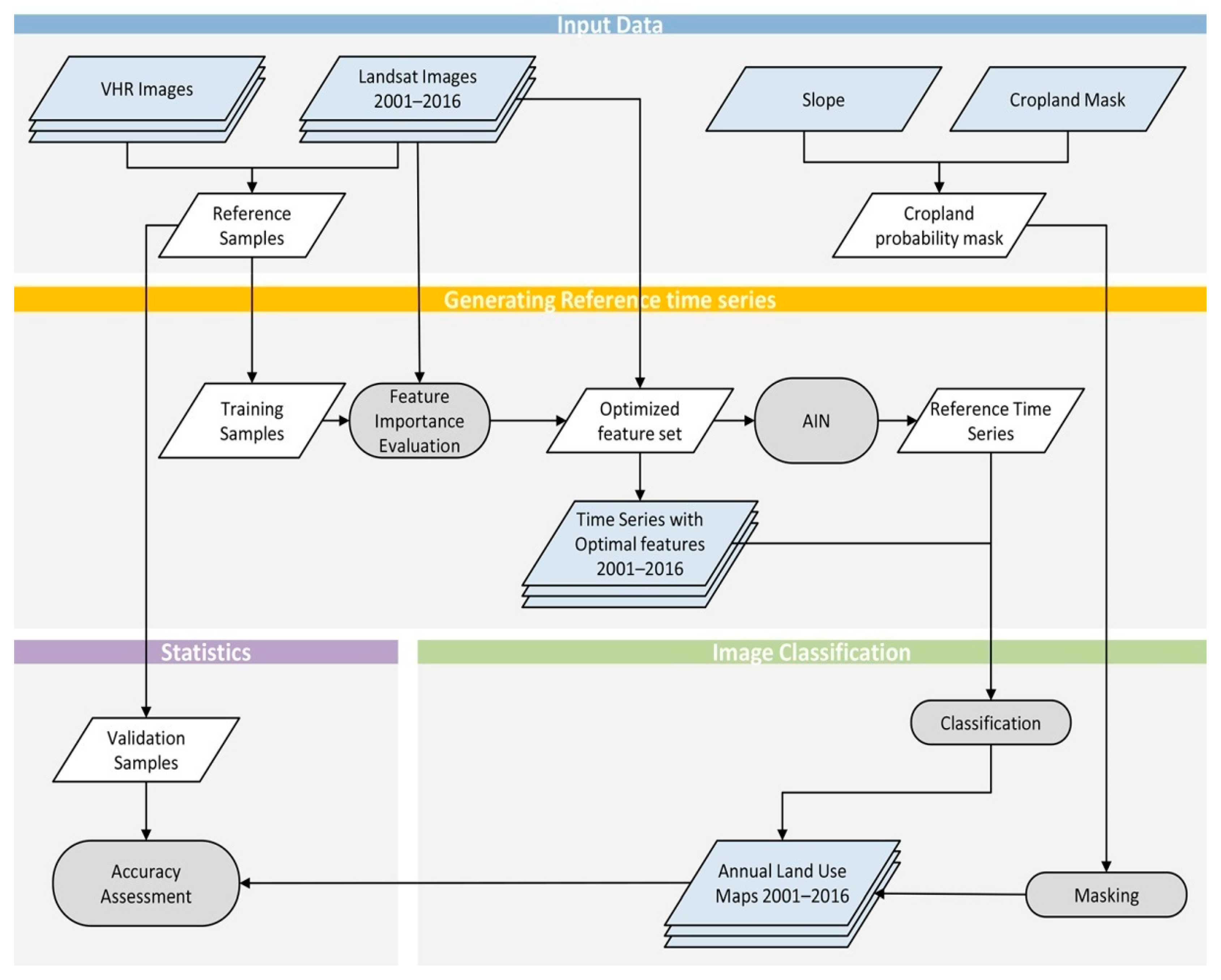
An overview of the methodology to create annual cropland maps is shown in Figure 2. Firstly, we extracted classification features from monthly composited Landsat time series data (Section 4.2), and then generated training and validation samples using both monthly composited Landsat image time series and high-resolution images (Section 4.3), respectively. We then used the Gini index importance score from the RF to evaluate the contribution of each feature for cropland identification, and selected two features as optimal features for cropland identification in each study site (Section 4.4). Next, we used the time series of the optimal features for the training samples in 2016 to generate reference time series using the artificial immune network (AIN) algorithm (Section 4.5), the possible cropland layer was generated from the DEM data in each study site (Section 4.6), and both reference time series and the possible cropland layer were used to identify cropland yearly between 2001 and 2016 (Section 4.7). Finally, the classification accuracies of cropland maps were assessed by the validation samples (Section 4.8), and the cropland acreage dynamics in the seven study sites were evaluated using the cropland maps generated in this study.
4.2. Compositing and Feature Extraction from Landsat Images
We used the Quality assurance (QA) band to mask the cloud pixels [41]. For Landsat-5 and Landsat-7 images, pixels with QA value equal to 66 and 68 remained as cloud pixels; for Landsat-8 images, pixels with QA value equal to 322, 324, 386 and 388 remained as cloud pixels. Next, monthly image time series were generated using the monthly maximum composition for the multi-spectral bands: blue, green, red, near-infrared (NIR), and two short-wave infrared (SWIR1 and SWIR2) bands; data availability generally increased from 2001 to 2016 (Figure 3). We then extracted two types of information from the monthly composited Landsat images: (i) information from the multi-spectral bands, and (ii) several vegetation indices calculated from the multi-spectral bands (see Table 2).
4.3. Collection of Reference Data
4.3.1. Collection of Training Data
To calibrate the classifier model (see Section 4.5), training samples (i.e., pixels) of five land-cover categories were collected in 2016: (i) Active Cropland (i.e., sown and harvested), (ii) Bareland, (iii) Grass/Shrub, (iv) Artificial Surface (e.g., built-up surface in urban regions), and (v) Water (e.g., rivers, lakes).
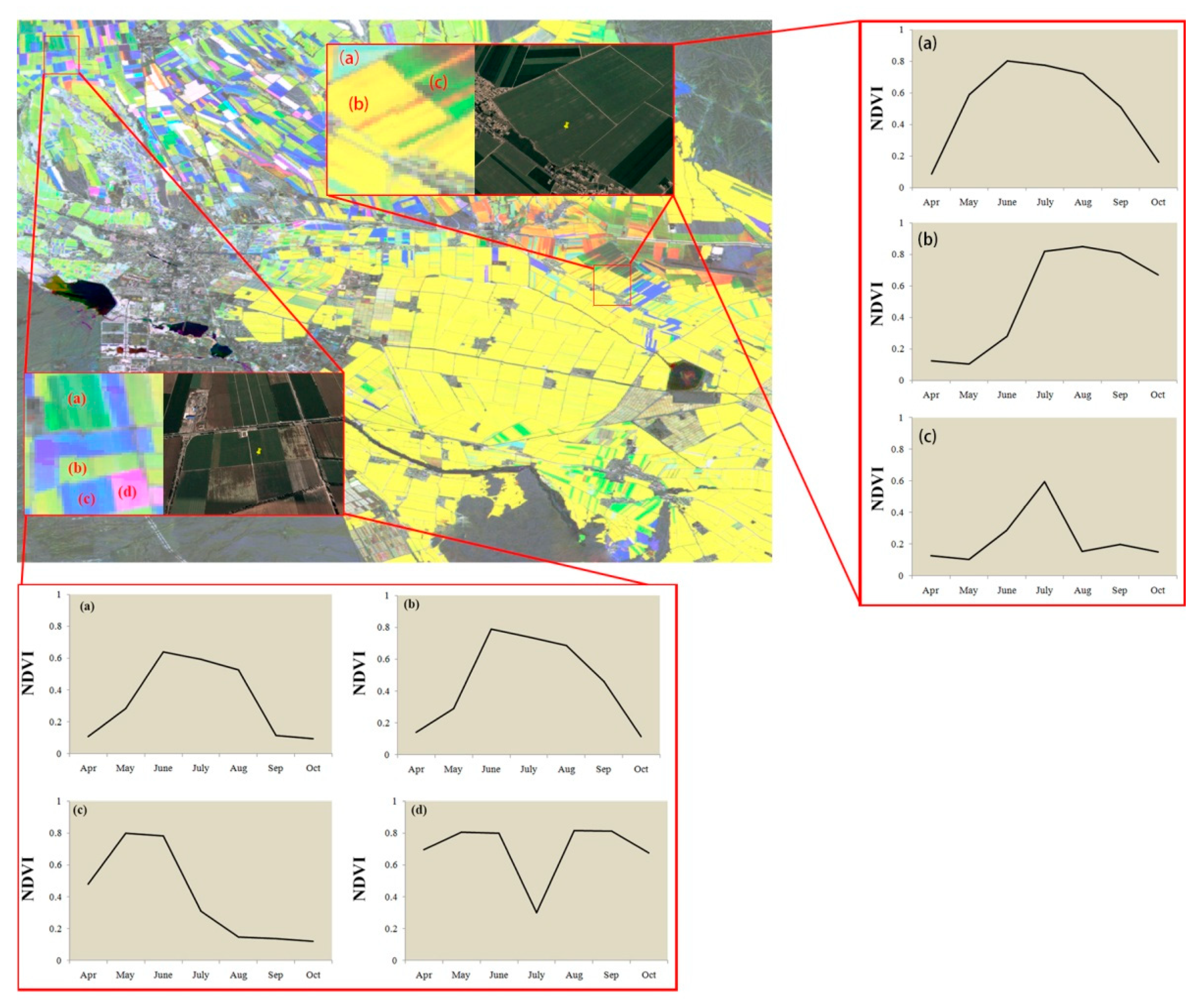
To acquire training pixels, we firstly collected polygons in regions of homogenous land cover, based on a visual inspection of very high resolution (VHR) images available on Google and Bing Maps. The polygons were cross-checked by interpreting Landsat NDVI time series (Figure 4). Next, the selected and cross-checked polygons were converted to 30-m pixels (Table 3). In addition, the training samples were mainly collected in 2016 because both Google/Bing Maps and 30-m NDVI time series had the best data availability for 2016. The collection of cropland samples had to consider the presence of multiple crop types (such as cotton, maize and wheat). Figure 5 shows training samples that represent cropland and their corresponding NDVI signatures.
4.3.2. Collection of Training Data
The validation focused on assessing the accuracy of the final, annual cropland maps that had a binary class legend, i.e., Cropland vs. Non-Cropland. This was done in order to ease the comparison of the accuracy of the maps with the existing products (see Section 3.2, which has different class legends). Validation samples were collected independently from the training samples using a random sampling approach. We first generated a random sample of 1000 pixels in each study site and year, respectively, using Hawth’s tool [47]. Landsat time series and VHR images were then used to visually interpret these validation samples (Table 4).
4.4. Feature Importance Estimation Using Random Forest
We used the Gini index generated from the random forest (RF) algorithm to select the optimal cropland identification features [48]. RF is an ensemble machine-learning technique that combines multiple trees [48]. Each tree is constructed using two-thirds of the training records and the remaining records are used for a test classification with an error referred to as an “out-of-bag error”. During the training procedure of RF, every time a split of a node is made on a variable, the Gini impurity criterion for the descendent nodes is less than that of the parent node. The importance score is the sum of the Gini decreases for each individual variable over all trees in the classification forest. In this research, the Gini importance score was obtained using the RandomForest package for R [49]. The number of trees in the ensemble was set to 1000 to allow convergence of the error statistic, and the number of features to split the nodes in the trees was set to the square root of the total number of input features [50].
For selecting optimal cropland identification features, we calculated the sum of the Gini scores of all seven temporal phases for each feature for each pair of land cover types (such as Cropland and Bareland). The calculations were repeated 10 times, and features with the highest average Gini score sum for each pair were calculated. Then, the two most important features were selected as optimal features for each study site. We only selected two features with a high contribution as optimal features because the low contribution feature will reduce the separability among different classes. Next, the time series of these two features were used to generate the reference time series for each study site.
4.5. Generating Reference Landsat Time Series
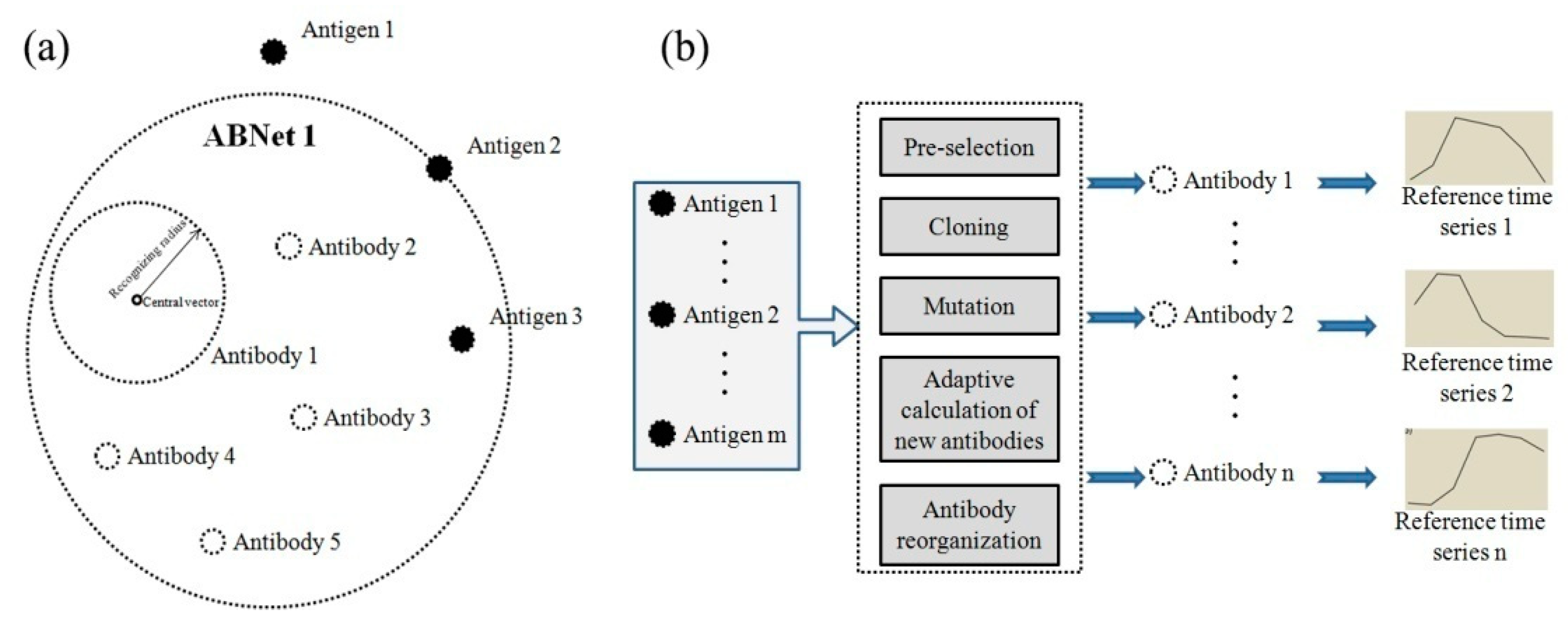
We used artificial immune network (AIN) algorithms (antibody network, ABNet) to generate the reference time series [51,52]. AIN methods are inspired by the human immune system, and these algorithms have shown good potential to solve pattern recognition problems. AIN-based algorithms call the input training samples “antigens”, and the “antibodies” were generated from the “antigens” to identify crop “antigens”, which is similar to the work of the human immune system. The training procedure of the AIN algorithms was to generate the “antibodies” using the training samples, and the classification procedure was to classify images (“new antigens”) and identify cropland using the “antibodies”. Generally, the antibodies contained three attributes: the crop type, central vector, and the recognizing radius (Figure 6a). In this study, the central vector of each antibody was defined as the reference time series. The procedures for generating the antibodies contain five steps: pre-selection, cloning, mutation, adaptive calculation of new antibodies, and antibody reorganization (Figure 6b) [53]. The first step (pre-selection) is to select an antigen as the preselected antigen, which could best represent the unrecognized antigen population. The second step (cloning) is to clone a large number of pre-selected antigens, and the third step (mutation) is to randomly mutate the cloned antigens and generate “possible antibodies”. The next step (adaptive calculating new artificial antibody) is to use all “possible antibodies” to recognize the “antigens”. The “possible antibody” which could identify the most recognized “antigens” were then defined as an “antibody”, and the “antigens” which could be identified by the “antibodies” were labeled as recognized “antigens”. Finally, the training procedure finished when all “antigens” were identified by “antibodies”. The advantage of AIN-based algorithms is that these algorithms can contain multiple “antibodies” that represent multiple situations of each land cover class, which is suitable for cropland mapping as cropland contains multiple crop types and the NDVI time series of cropland have standard derivations (see Figure 5). In this study, the time series of the two optimal features (Section 4.1) of the training samples were used as antigens to generate the antibodies. The Euclidean distance was selected as the similarity measure because it is easily calculated [54].
4.6. Annual Cropland Identification
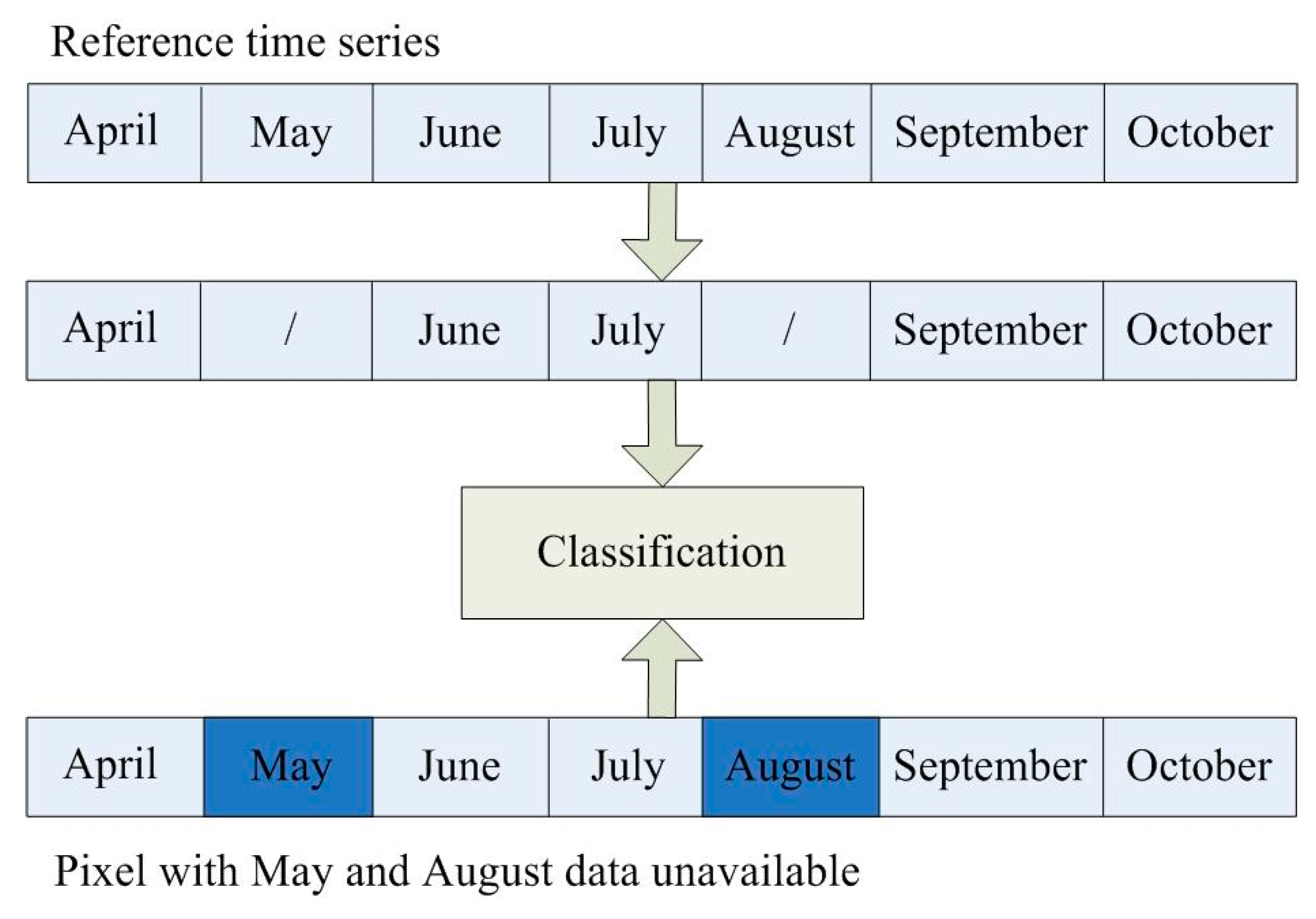
We used the reference time series to identify cropland between 2001 and 2016 annually. The classification procedure was to calculate the Euclidean distance between the vector of a pixel and the optimal feature time series of each reference time series, and the pixel was labeled as the land cover type of the antibody with the minimum distance. We were able to improve this method and solve the “missing data” problem. For example, among the seven time phases we applied in this study, if a pixel had five available time phases, we could extract the values at the “high-quality” time phase and identify the pixel with “missing data” (Figure 7). After that, we merged the Shrub/grass, Bareland, Water, and Artificial Surface as non-cropland and generated the binary cropland extent maps.
4.7. Generating Possible Cropland Layer
We used the AWAD30 DEM data to calculate the slope of the terrain in each study area, and we defined pixels with a slope of less than 15 degrees as “potential cropland” area [55,56]. This binary mask was finally used to post-process the annual cropland maps; only pixels having less than 15 degrees were possible to be classified as cropland according to Chinese cultivated land regulation [57].
4.8. Accuracy Assessment
We used metrics from the confusion matrix to assess the quality of the annual cropland maps [58]. These include the producer’s accuracy (PA), user’s accuracy (UA), overall accuracy (OA), and Kappa coefficient of variation (kappa). All these accuracy metrics were calculated from the validation samples. In addition to this, we evaluated the accuracy of existing cropland layers, FROM-GLC, and Globaland30 in 2010. We applied McNemar’s test to evaluate the pair-wise statistical significance of the difference in accuracy between FROM-GLC, Globaland30, and RBM-based maps in 2010 [59]. McNemar’s test is a non-parametric test based on the standardized normal test statistic, as in Equation (1):
where f12 is the number of samples that are correctly classified by classifier 1 and incorrectly classified by classifier 2. We defined three cases of differences in accuracy between classifier 1 and classifier 2 according to McNemar’s test:
- No significance between classifiers 1 and 2 (N): −1.96 < Z < 1.96.
- Positive significance (classifier 1 has higher accuracy than classifier 2) (S+): Z > 1.96.
- Negative significance (classifier 1 has lower accuracy than classifier 2) (S−): Z < −1.96.
5. Results
5.1. Feature Selection
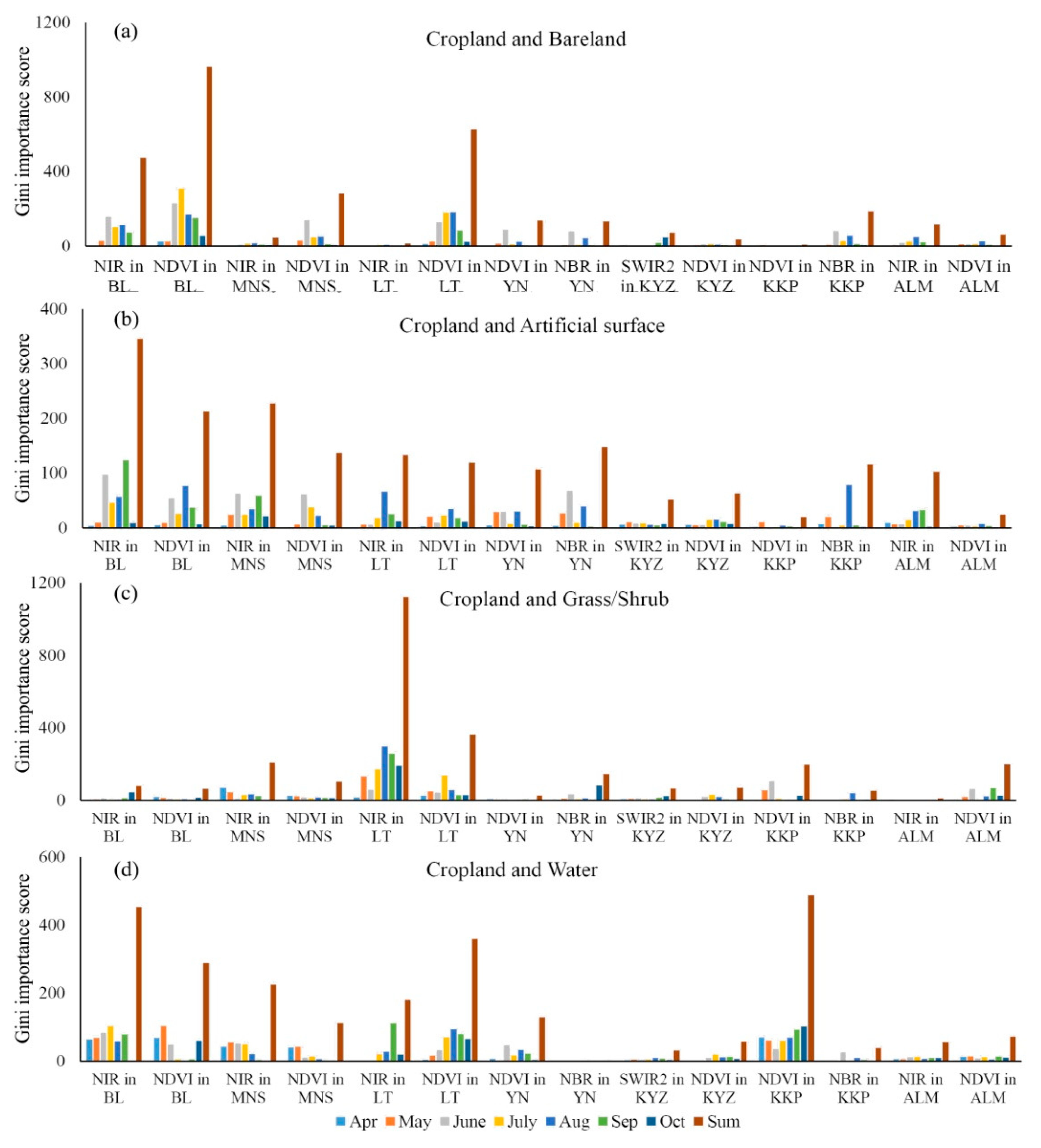
Figure 8 shows optimal features in all seven study sites and pair-wise; the Gini importance scores for all features are shown in the Supporting Material Tables S1–S7. Among all features, NIR, SWIR2, NDVI, and NBR are selected, and the NDVI is selected in all seven study sites. Among all land cover types, NDVI shows good potential to identify Cropland from Bareland and Water. For Cropland and Bareland, the Gini importance scores of June NDVI in BL and August NDVI in YN are 307.61 and 179.75, respectively. For Cropland and Water, the Gini score sums of the NDVI are 359.84 and 487.57 in YN and KKP, respectively. For separating Cropland from Artificial and Grass/Shrub, the Gini scores of NDVI are lower; for instance, the Gini score sums of NDVI in BL and MNS are 213.22 and 136.78. Besides the NDVI, the NIR band is selected as the optimal feature in BL, MNS, LT, and ALM. The NIR shows potential to discriminate Cropland from Bareland, Water, Artificial Surface, and Grass/Shrub; the Gini score sums of NIR for Cropland and Grass/Shrub are 207.97 and 1120.44, respectively, which are higher than the NDVI Gini score sums (136.78 and 104.18). NBR is selected in YN and KKP, as NBR has a high Gini score when identifying Cropland from Artificial Surface and Grass/Shrub; the Gini score sums are 147.6 and 145.25 for separating Cropland and Artificial Surface and Cropland and Grass/Shrub in YN, respectively. SWIR2 is selected in KYZ, with the Gini score sums being 51.29 and 66.55 for separating Cropland and Artificial Surface, and Cropland and Grass/Shrub, respectively.
5.2. Accuracy Assessment of the Annual Crop Maps
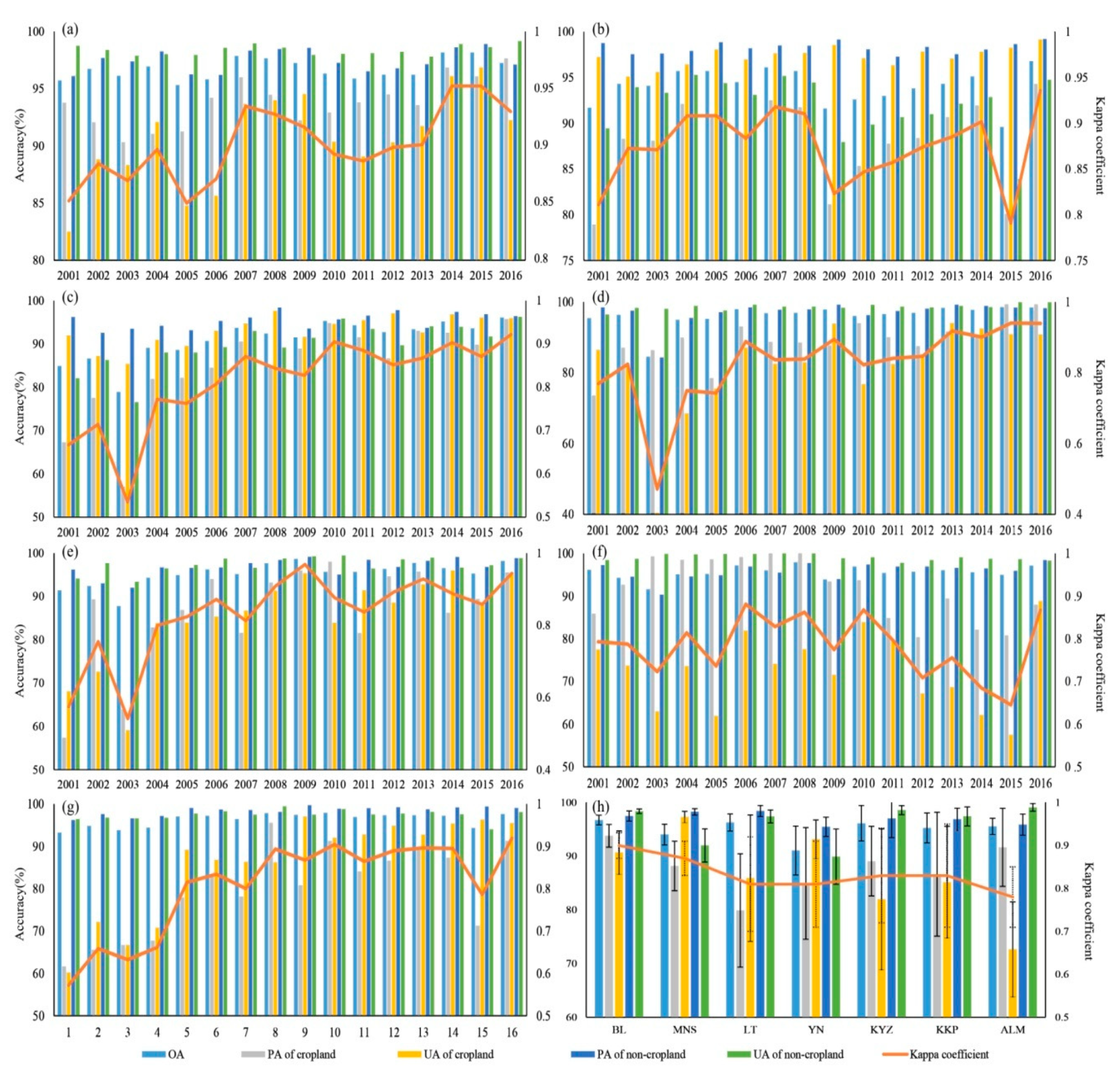
The reference time series acquired by the training samples of 2016 show good potential to identify croplands. This is evidenced by the generally high overall classification accuracies (>90%) that this method achieved in most landscapes and years (Figure 9). In BL and MNS, both producer’s accuracy (PA) and user’s accuracy (UA) of Cropland are higher than 85% after 2002. Figure S1 shows a representative region in BL. The agricultural landscapes in BL are typically rectangular mosaic crop fields and the cropland distribution maps showed clear field boundaries. The cropland expanded between 2005 and 2015, as described by the cropland distribution map. In MNS, rectangular crop fields show clear field boundaries, but heterogeneous fields have some speckle noise on the cropland maps. The misclassified pixels are mainly mixed pixels, NIR, and NDVI, and profiles of the mixed pixels are different from the reference profiles (Figure S2).
The classification accuracies of the other five study sites are lower than BL and MNS. In Luntai, the PAs of Cropland are higher than 85% in only six years, and the UAs of Cropland are higher than 85% between 2005 and 2016. The crop fields in LT are characterized by small field size, and the mixed pixels lead to low classification accuracy (Figure S3). Classification accuracy is low between 2001 and 2004; both PAs and UAs are lower than 70%. This is because the images were not acquired monthly over these four years. For example, in south LT, only satellite observations of September were acquired in 2002, and the images in September cannot separate Grass/Shrub from Cropland. Although some stripes were observed in the Landsat NDVI time series, cropland maps are not affected. In YN, the PA of Cropland is higher than 85% between 2006 and 2016, and the UA of Cropland is higher than 85% for the 16 years (Figure 9). Cropland could be identified in a homogenous area, and the extension of the cropland during 2006 and 2016 could be extracted (Figure S4). In KYZ and KKP, both the UAs and PAs are higher than 85% between 2006 and 2016. The low classification accuracies before 2005 are mainly due to the missing image time series. For example, only two time phases between April and October were acquired in KYZ. While the field sizes are small in KKP, the croplands are cross-distributed with in-rotation fields, which led to the misclassification of cropland. Classification accuracies of cropland are low in ALM; the UAs are higher than 80% only in 2006, 2010, and 2016 (Figure 9). The low UAs are mainly because of the confusion among Cropland, Grass/Shrub, and Bareland. Figure S5 shows that NDVI time series of some winter crops are similar to Bareland, which are abandoned fields. Crops with a long growing season have similar NDVI times series to vegetation in the mountain area; only fields with summer crops are correctly identified.
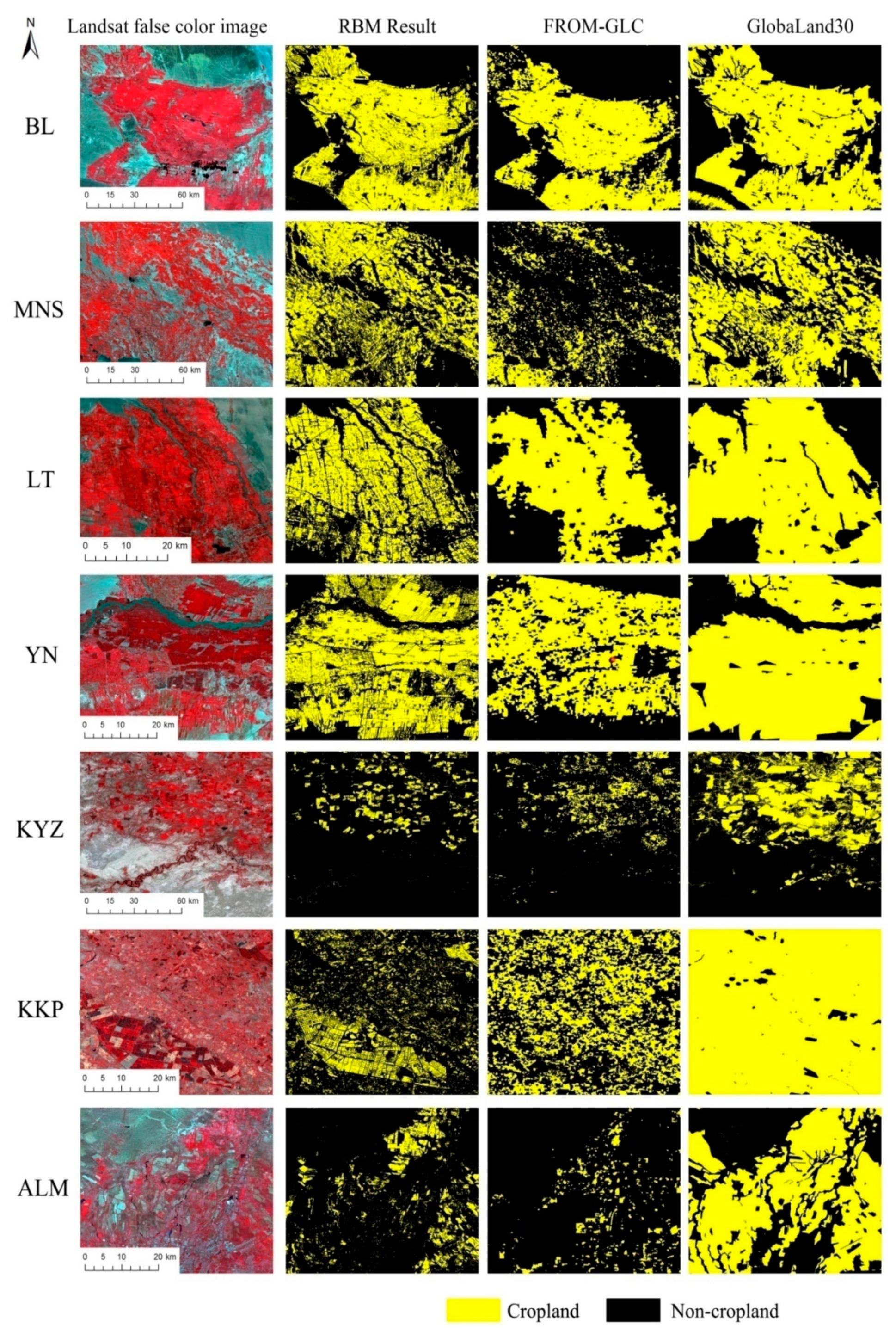
5.3. Comparison with Existing 30-m Land-Cover Products
We compared the classification result of RBM and two existing 30-m land-cover products, FROM-GLC and GlobaLand30 in 2010, by classification accuracy comparison (Table 5), McNemar’s test (Table 6) and wall-to-wall comparison (Figure 10). All three products generate accurate cropland maps in BL with overall classification accuracies being higher than 95%, and PAs and UAs higher than 90%. For the other six study sites, the RBM outperforms the two existing products. In MNS, YN and KYZ, PAs of RBM were similar to GlobaLand30, and the UAs of RBM were slightly higher. Also, the accuracy of RBM was slightly higher than FROM–GLC in LT and KKP. In ALM, the UA of RBM was significantly higher than GlobaLand30 and FROM–GLC.
Table 6 shows that RBM significantly outperforms Globaland30 in KKP and KYZ, and outperforms FROM–GLC in MNS, ALM, KKP, and KYZ. From the wall-to-wall comparison, RBM was able to identify crop field boundaries. Note that FROM–GLC and GlobaLand30 cannot identify the roads between the cropland fields, particularly in LT and YN. In addition, RBM identifies the homogenous cropland in KKP and ALM, but FROM–GLC and GlobaLand30 fail to map these cropland fields, while RBM and FROM–GLC fail to identify the fragmented croplands in the region, and GlobaLand30 overestimates the fragmented cropland.
5.4. Land Use Intensity Change between 2001 and 2016
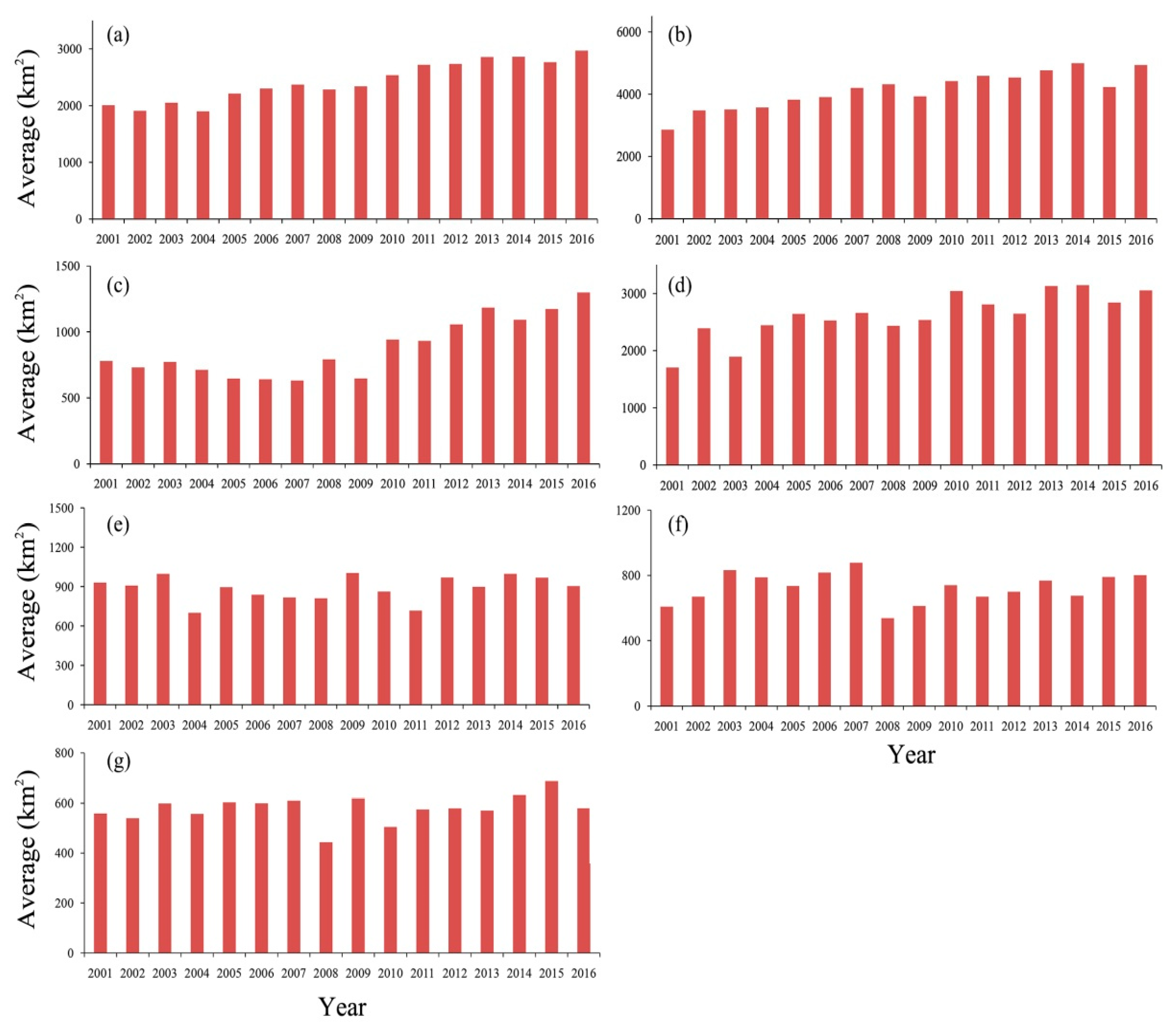
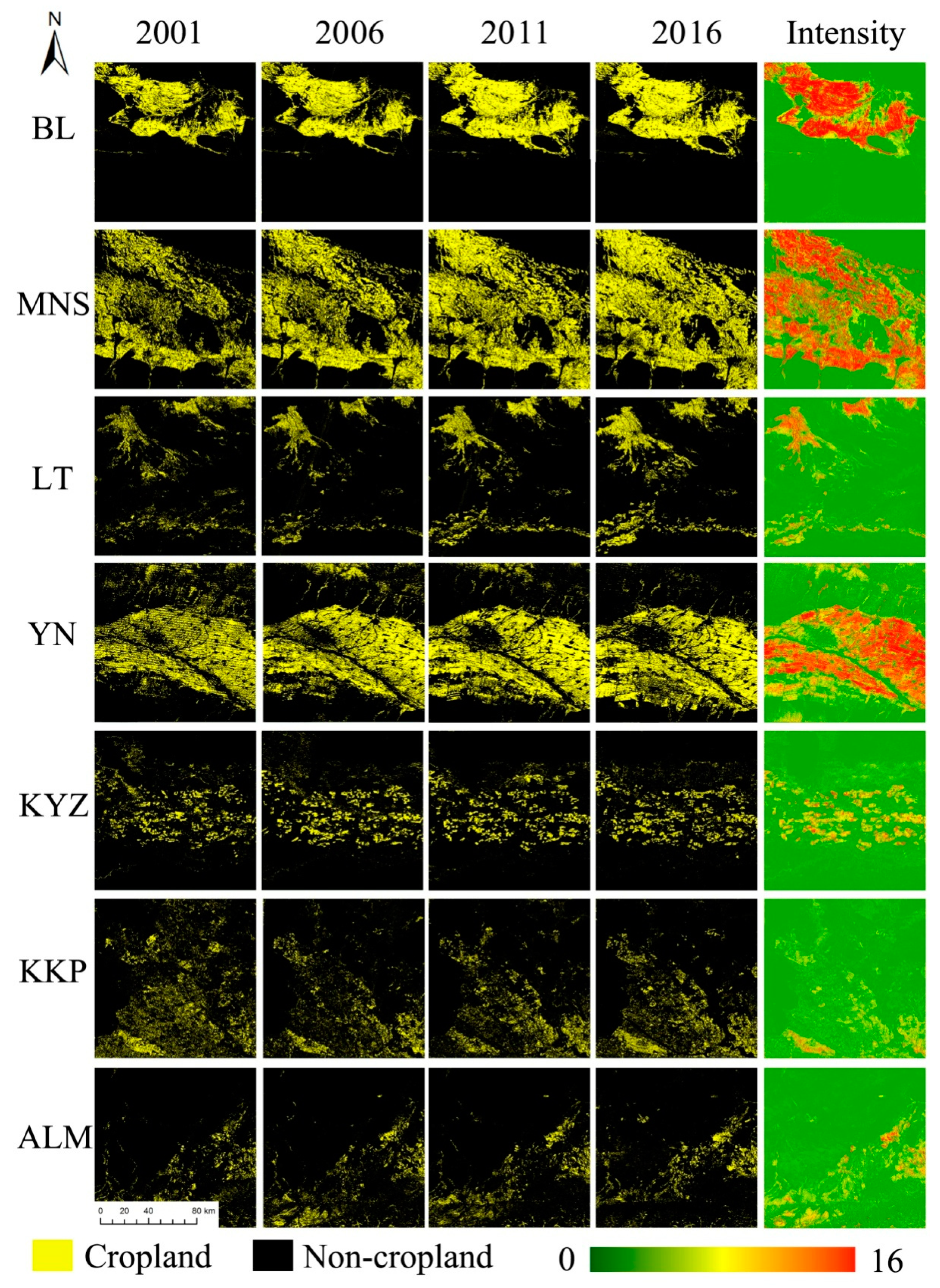
We used the annual cropland map generated from RBM to analyze the cropland change between 2001 and 2016. In the four study sites in Xinjiang, cropland acreage shows an increasing trend. Between 2002 and 2016, cropland acreage increases from 2007 km2 to 2970 km2 in BL, and between 2001 and 2016, it increases from 2858 km2 to 4930 km2 in MNS. In LT, cropland acreage increases from 780 km2 to 1299 km2 between 2001 and 2016, and from 1704 km2 to 3053 km2 in YN (Figure 11). Figure 11 shows the cropland intensity between 2001 and 2016. The cropland intensity of most cropland in these four study regions is higher than 15, and yellow patterns are the cropland expended between 2001 and 2016. Generally, cropland extended as Bareland is transformed to Cropland; croplands do not expand into the other three study regions. The cropland acreage is around 700–900 km2 in KYZ, 600–800 km2 in KKP, and around 500–600 km2 in ALM. Figure 12 shows that the cropland intensities of the crop fields in these study regions are around 8 during the 16-year period, which means that the fields are in rotation and there is no clear expansion or shrink trend.
6. Discussion
This study proposed a reference time-series-based method to automatically generate the annual cropland extent at 30-m resolution. The “core” of the method is the “reference time series”. The first challenge was to collect training samples which were used to generate the reference time series. As “Cropland” contains multiple crop types, the training samples of the major crop types should be included in the training samples data set. We used images of May, July and September Landsat NDVI to collect training samples for “Cropland”. Different vegetation is shown as different colors in this composed image (Figure 4); for example, winter crops (such as winter wheat) is blue and cotton is yellow. Samples for each color were then selected as “Cropland” training samples to ensure sample richness.
The image time series are essential for cropland mapping, but another challenge in deriving annual cropland maps at 30-m spatial resolution is that regular image time series cannot be acquired, particularly before 2010. We then used the monthly composition strategy to generate the monthly Landsat images, as this strategy made use of all available Landsat pixels. Although the monthly composition reduced the “no data” pixels in the Landsat time series, some time series were still “irregular”. For example, some pixels of 2007 in LT showed serious “stripe noise” due to the Landsat-7 images (Figures S3 and S4). In this case, most classifier and standard cluster methods cannot process the irregular time series with missing values. However, the reference time-series-based method proposed in this study contributes to classifying cropland with irregular image time series. Reference time series are derived from the training samples in 2016, and sample pixels acquired Landsat records in all seven months. To identify an irregular time series, we can extract a subset of reference image time series corresponding to the “good quality” temporal phases in the irregular time series, and then identify cropland by comparing the subset reference time series and the image time series. Therefore, although some “stripe noise” or missing data is in the Landsat time series, the cropland map is not affected by this noise (Figures S3 and S4).
The optimal features selected in this study are mainly the NDVI and NIR bands. The NBR and SWIR2 bands were selected in KYZ and KKP. NDVI made the most contribution to identifying “Cropland” from “Bareland”, “Artificial Surface” and Water, while the NIR band contributed to distinguishing “Cropland” from “Shrub/Grass”. This is consistent with Zhu and Woodcock [60] in that NIR and SWIR time series showed large differences when pixels changed from forest to agricultural land. Additionally, images in some important temporal phases are essential for cropland mapping, and the May to August images have a high Gini score sum in this study (Tables S1–S7), which is consistent with the growing season of the major crop types in the study sites. For example, winter crops (such as winter wheat) have high NDVI in May, and cotton and maize have NDVI peaks in July [24,61]. Thus, acquiring optimal features at important temporal phases contributes to correct cropland identification. We selected two features to generate reference time series, although NDVI was selected in all seven study sites and the NIR band was selected in four sites; the optimal features may vary in different regions. Generally, the optimal feature could distinguish “Cropland” and “Shrub/Grass”, and in different study regions, different vegetation types led to variation of the optimal features. When applying this method in a large area, feature contribution should be carefully evaluated to ensure that the selected feature time series were representative of the major vegetation types in the study area.
Seven study sites were used to evaluate the method proposed in this study, and we generated high classification accuracies in BL, MNS, YN, and KYZ, but low classification accuracy in ALM, LT, and KKP, which means RBM still has some uncertainty for cropland extent mapping. There are several reasons for the uncertainty: (1) The small field size in some study regions. Generally, small field size leads to mixed pixels with the mixed signature of multiple crop types [62]. As a result, the mixed time series do not match any reference time series and lead to the wrong classification (Figure S2). Low and Duveiller [63] quantitatively assessed the effect of pixel size on uncertainty and found that regions with heterogeneous landscapes (such as KKP) have higher classification uncertainty, due to the decrease of pixel purity and increasing number of mixed pixels. (2) Images at the important temporal phases were not acquired. There are some serious data missing and only a limited number of Landsat records were acquired, for example, in 2003 for Bole and 2002 for YN. When all features of the important temporal phases are missing, the reference time series failed to extract cropland. (3) The confusion between “Cropland” and other land cover types. There were “Cropland” and “Shrub/Grass” that had similar NDVI and NIR time series in ALM (Figure S5), and the confusion led to misclassification. (4) The representativeness of training samples. As we used the training samples to generate reference time series, if the NDVI time series of some typical crop types were not recorded in the training samples, the RBM could not identify cropland with these typical crops and this led to misclassification. (5) Although the slope layer derived from a DEM was included to mask the vegetation in the mountain area, the shrub and grass in flat regions were still misclassified as cropland.
7. Conclusions
Generating yearly cropland distributions at 30-m resolution is challenging because Landsat time series are not acquired regularly, and training samples need to be collected annually. In this paper, we presented a method to generate annual cropland distribution maps using reference image time series, which could handle the irregular Landsat time series. The method was evaluated in seven study sites (BL, MNS, LT, YN, KKP, KYZ, and ALM). The main conclusions are as follows:
- (1)
- The reference time series method showed good potential to identify “irregular” Landsat time series and generate annual cropland distribution. Classification accuracies of the Cropland are higher than 85% in most cases. However, mixed pixels caused by small field size, the loss of image at important temporal phases and signature confusion between “Cropland” and other land cover types led to misclassification.
- (2)
- The NDVI, NBR, NIR and SWIR2 bands were selected as optimal features for cropland mapping in 2016, and NDVI was selected as the most important feature.
- (3)
- The annual cropland maps created in this study are a useful basis for monitoring cropland distribution dynamics. Both wall-to-wall comparison and acreage statistics showed that the cropland expanded significantly in BL, MNS, and YN during the past 16 years, and the cropland in these four study regions had high cropland intensity. The cropland acreage in KYZ, KKP, and ALM have lower cropland intensity as the fields in these study regions were in rotation, and no clear expansion or shrinkage trends were observed.
The reference time-series-based method showed good potential to generate continuous cropland extent maps annually. Future work should focus on using images with a better spatial resolution to identify the cropland with small fields. Additionally, more features, derived from SAR and LiDAR sensors, should be considered to further solve the confusion between “Cropland” and other natural vegetation.
Supplementary Materials
The following are available online at https://0-www-mdpi-com.brum.beds.ac.uk/2072-4292/10/12/2057/s1. Figure S1: Cropland distributions of two sub-regions in BL. Figure S2: Cropland distributions of sub-regions in MNS. Figure S3: Cropland distributions of sub-regions in LT. Figure S4: Cropland distributions of sub-regions in YN. Figure S5: Some of the Cropland, Bareland and Grass/Shrub NDVI time series. Table S1: Gini Importance scores for different time phases and features (BL). Table S2: Gini Importance score for different time phases and features (MNS). Table S3: Gini Importance scores for different time phases and features (LT). Table S4: Gini Importance scores for different time phases and features (YN). Table S5: Gini Importance score for different time phases and features (KYZ). Table S6: Gini Importance scores for different time phases and features (KKP). Table S7: Gini Importance score for different time phases and features (ALM).
Author Contributions
P.H. validation, formal analysis; P.H. and F.L. conceptualization and methodology; P.H., F.L. and C.B. writing—review and editing.
Funding
This research was funded by China Postdoctoral Science Foundation funded project, grant number 2017M620075 and BX201700286 and National Natural Science Foundation of China, grant number 41801359. And The APC was funded by China Postdoctoral Science Foundation funded project, grant number 2017M620075.
Acknowledgments
The authors thanks Google Earth Engine for providing cloud computation service.
Conflicts of Interest
The authors declare no conflict of interest.
References
- Lambin, E.F.; Meyfroidt, P. Global land use change, economic globalization, and the looming land scarcity. Proc. Natl. Acad. Sci. USA 2011, 108, 3465–3472. [Google Scholar] [CrossRef] [PubMed] [Green Version]
- Justice, C.O.; Becker-Reshef, I. Report from the Workshop on Developing a Strategy for Global Agricultural Monitoring in the Framework of Group on Earth Observations; FAO: Rome, Italy, 2007. [Google Scholar]
- Smaliychuk, A.; Müller, D.; Prishchepov, A.V.; Levers, C.; Kruhlov, I.; Kuemmerle, T. Recultivation of abandoned agricultural lands in Ukraine: Patterns and drivers. Glob. Environ. Chang. 2016, 38, 70–81. [Google Scholar] [CrossRef]
- JICA. The Study on Regional Development in Karakalpakstan in the Republic of Uzbekistan (Progress Report); JICA: Tokyo, Japan.
- Ramankutty, N.; Foley, J.A. Estimating historical changes in global land cover: Croplands from 1700 to 1992. Glob. Biogeochem. Cycles 1999, 13, 997–1027. [Google Scholar] [CrossRef] [Green Version]
- Löw, F.; Prishchepov, A.V.; Waldner, F.; Dubovyk, O.; Akramkhanov, A.; Biradar, C.; Lamers, J.P.A. Mapping cropland abandonment in the aral sea basin with modis time series. Remote Sens. 2018, 10, 159. [Google Scholar] [CrossRef]
- Prishchepov, A.V.; Müller, D.; Dubinin, M.; Baumann, M.; Radeloff, V.C. Determinants of agricultural land abandonment in post-soviet European Russia. Land Use Policy 2013, 30, 873–884. [Google Scholar] [CrossRef]
- Bahadur, K.C.K. Spatio-temporal patterns of agricultural expansion and its effect on watershed degradation: A case from the mountains of Nepal. Environ. Earth Sci. 2012, 65, 2063–2077. [Google Scholar] [CrossRef]
- Spera, S.A.; Galford, G.L.; Coe, M.T.; Macedo, M.N.; Mustard, J.F. Land-use change affects water recycling in brazil’s last agricultural frontier. Glob. Chang. Biol. 2016, 22, 3405–3413. [Google Scholar] [CrossRef] [PubMed]
- Bernauer, T.; Siegfried, T. Climate change and international water conflict in central Asia. J. Peace Res. 2012, 49, 227–239. [Google Scholar] [CrossRef]
- Friedl, M.A.; McIver, D.K.; Hodges, J.C.F.; Zhang, X.Y.; Muchoney, D.; Strahler, A.H.; Woodcock, C.E.; Gopal, S.; Schneider, A.; Cooper, A.; et al. Global land cover mapping from modis: Algorithms and early results. Remote Sens. Environ. 2002, 83, 287–302. [Google Scholar] [CrossRef]
- ESA Globcover. Available online: http://due.esrin.esa.int/page_globcover.php (accessed on 12 December 2018).
- Waldner, F.; Hansen, M.C.; Potapov, P.V.; Löw, F.; Newby, T.; Ferreira, S.; Defourny, P. National-scale cropland mapping based on spectral-temporal features and outdated land cover information. PLoS ONE 2017, 12, e0181911. [Google Scholar] [CrossRef] [PubMed]
- Gong, P.; Wang, J.; Yu, L.; Zhao, Y.C.; Zhao, Y.Y.; Liang, L.; Niu, Z.G.; Huang, X.M.; Fu, H.H.; Liu, S.; et al. Finer resolution observation and monitoring of global land cover: First mapping results with landsat tm and etm+ data. Int. J. Remote Sens. 2013, 34, 2607–2654. [Google Scholar] [CrossRef]
- NGCC. Global Land Cover Mapping at 30 m Resolution. Available online: http://ngcc.sbsm.gov.cn/article/en/ps/mp/201302/20130200001694.shtml (accessed on 12 December 2018).
- Xiong, J.; Thenkabail, P.; Tilton, J.; Gumma, M.; Teluguntla, P.; Oliphant, A.; Congalton, R.; Yadav, K.; Gorelick, N. Nominal 30-m cropland extent map of continental Africa by integrating pixel-based and object-based algorithms using sentinel-2 and landsat-8 data on google earth engine. Remote Sens. 2017, 9, 1065. [Google Scholar] [CrossRef]
- Ju, J.C.; Roy, D.P. The availability of cloud-free landsat etm plus data over the conterminous united states and globally. Remote Sens. Environ. 2008, 112, 1196–1211. [Google Scholar] [CrossRef]
- Löw, F.; Biradar, C.; Dubovyk, O.; Fliemann, E.; Akramkhanov, A.; Vallejo, A.N.; Waldner, F. Regional-scale monitoring of cropland intensity and productivity with multi-source satellite image time series. GIScience Remote Sens. 2017, 55. [Google Scholar] [CrossRef]
- Wu, M.; Wu, C.; Huang, W.; Niu, Z.; Wang, C.; Li, W.; Hao, P. An improved high spatial and temporal data fusion approach for combining landsat and modis data to generate daily synthetic landsat imagery. Inf. Fusion 2016, 31, 14–25. [Google Scholar] [CrossRef]
- Knauer, K.; Gessner, U.; Fensholt, R.; Forkuor, G.; Kuenzer, C. Monitoring agricultural expansion in Burkina Faso over 14 years with 30 m resolution time series: The role of population growth and implications for the environment. Remote Sens. 2017, 9, 132. [Google Scholar] [CrossRef]
- Liu, J.; Kuang, W.; Zhang, Z.; Xu, X.; Qin, Y.; Ning, J.; Zhou, W.; Zhang, S.; Li, R.; Yan, C.; et al. Spatiotemporal characteristics, patterns, and causes of land-use changes in china since the late 1980s. J. Geogr. Sci. 2014, 24, 195–210. [Google Scholar] [CrossRef]
- Zhong, L.H.; Gong, P.; Biging, G.S. Efficient corn and soybean mapping with temporal extendability: A multi-year experiment using landsat imagery. Remote Sens. Environ. 2014, 140, 1–13. [Google Scholar] [CrossRef]
- Yan, L.; Roy, D.P. Automated crop field extraction from multi-temporal web enabled landsat data. Remote Sens. Environ. 2014, 144, 42–64. [Google Scholar] [CrossRef]
- Hao, P.; Wang, L.; Zhan, Y.; Wang, C.; Niu, Z.; Wu, M. Crop classification using crop knowledge of the previous year: Case study in southwest Kansas, USA. Eur. J. Remote Sens. 2016, 49, 1061–1077. [Google Scholar] [CrossRef]
- Hao, P.; Wang, L.; Zhan, Y.; Niu, Z. Using moderate-resolution temporal Ndvi profiles for high-resolution crop mapping in years of absent ground reference data: A case study of bole and Manas counties in Xinjiang, China. ISPRS Int. Geo-Inf. 2016, 5, 67. [Google Scholar] [CrossRef]
- Zhong, L.; Hu, L.; Yu, L.; Gong, P.; Biging, G.S. Automated mapping of soybean and corn using phenology. ISPRS J. Photogramm. Remote Sens. 2016, 119, 151–164. [Google Scholar] [CrossRef] [Green Version]
- Waldner, F.ß.; Canto, G.S.; Defourny, P. Automated annual cropland mapping using knowledge-based temporal features. ISPRS J. Photogramm. Remote Sens. 2015, 110, 1–13. [Google Scholar] [CrossRef]
- Saiko, T.A.; Zonn, I.S. Irrigation expansion and dynamics of desertification in the circum-aral region of central Asia. Appl. Geogr. 2000, 20, 349–367. [Google Scholar] [CrossRef]
- Meyfroidt, P.; Schierhorn, F.; Prishchepov, A.V.; Müller, D.; Kuemmerle, T. Drivers, constraints and trade-offs associated with recultivating abandoned cropland in Russia, Ukraine and Kazakhstan. Glob. Environ. Chang. 2016, 37, 1–15. [Google Scholar] [CrossRef] [Green Version]
- Xu, Y.; Yang, J.; Li, W.; Fang, G.; Zhang, S.; Deng, H.; Dong, J. Spatial-temporal change in different vegetation growth of Xinjiang from 1982 to 2013. Acta Pratacult. Sin. 2016, 25, 47–63. [Google Scholar] [CrossRef]
- Yuan, Y.; Liu, H.; Li, B.; Gao, X.; Xu, L.; Dong, G. Study on the change of ecosystem in Xinjiang from 2000 to 2010. J. Geo-Inf. Sci. 2015, 17, 300–308. [Google Scholar]
- Lu, Q.; Liu, L.; Wang, Y.; Li, Y. Landscape pattern change and its driving forces in agricultural oasis of Sangong river basin in Xinjiang, northwest china in recent 30 years. Chin. J. Ecol. 2013, 32, 748–754. [Google Scholar]
- Wang, S.; Wang, S. Land use/land cover change and their effects on landscape patterns in the Yanqi basin, Xinjiang (China). Environ. Monit. Assess. 2013, 185, 9729–9742. [Google Scholar] [CrossRef] [PubMed]
- Zhao, Z.; Qiao, M.; Wu, S.; Tian, C. Cultivated land resources security of oases and its conservation strategies in Xinjiang. Arid. Land Geogr. 2010, 33, 1019–1025. [Google Scholar]
- Fan, Z.; Yu, P.; Qiao, M.; Xu, H.; Zhang, P.; Zhang, Q.; Fu, J. Comprehensive improvement of cultivated land for ecological protection to agriculture in arid areas: A case of Manasi river basin of Xinjiang. Arid. Land Geogr. 2012, 35, 772–777. [Google Scholar]
- Siegfried, T.; Bernauer, T.; Guiennet, R.; Sellars, S.; Robertson, A.W.; Mankin, J.; Bauergottwein, P.; Yakovlev, A. Will climate change exacerbate water stress in central Asia? Clim. Chang. 2012, 112, 881–899. [Google Scholar] [CrossRef]
- Yu, L.; Wang, J.; Clinton, N.; Xin, Q.; Zhong, L.; Chen, Y.; Gong, P. From-gc: 30 m global cropland extent derived through multisource data integration. Int. J. Digit. Earth 2013, 6, 521–533. [Google Scholar] [CrossRef]
- Chen, J.; Chen, J.; Liao, A.; Cao, X.; Chen, L.; Chen, X.; He, C.; Han, G.; Peng, S.; Lu, M. Global land cover mapping at 30 m resolution: A pok-based operational approach. ISPRS J. Photogramm. Remote Sens. 2015, 103, 7–27. [Google Scholar] [CrossRef]
- JAXA. Alos Global Digital Surface Model “Alos World 3d-30m” (aw3d30). Available online: http://www.eorc.jaxa.jp/ALOS/en/aw3d30/index.htm (accessed on 31 October 2018).
- Hu, Z.; Peng, J.; Hou, Y.; Shan, J. Evaluation of recently released open global digital elevation models of Hubei, china. Remote Sens. 2017, 9, 262. [Google Scholar] [CrossRef]
- Gorelick, N.; Hancher, M.; Dixon, M.; Ilyushchenko, S.; Thau, D.; Moore, R. Google earth engine: Planetary-scale geospatial analysis for everyone. Remote Sens. Environ. 2017, 202, 18–27. [Google Scholar] [CrossRef]
- Rouse, J.W.; Haas, R.H.; Schell, J.A.; Deering, D.W.; Harlan, J.C. Monitoring the Vernal Advancements and Retrogradation of Natural Vegetation; NASA/GSFC: Washiongton, DC, USA, 1974; pp. 1–137.
- Lopez Garcia, M.J.; Caselles, V. Mapping burns and natural reforestation using thematic mapper data. Geocarto Int. 1991, 6, 31–37. [Google Scholar] [CrossRef]
- Gao, B.C. Ndwi—A normalized difference water index for remote sensing of vegetation liquid water from space. Remote Sens. Environ. 1996, 58, 257–266. [Google Scholar] [CrossRef]
- Gitelson, A.A.; Kaufman, Y.J.; Stark, R.; Rundquist, D. Novel algorithms for remote estimation of vegetation fraction. Remote Sens. Environ. 2002, 80, 76–87. [Google Scholar] [CrossRef] [Green Version]
- Salomonson, V.V.; Appel, I. Estimating fractional snow cover from modis using the normalized difference snow index. Remote Sens. Environ. 2004, 89, 351–360. [Google Scholar] [CrossRef]
- Hawthorne, B. Hawth’s Analysis Tools for Arcgis. Available online: http://www.spatialecology.com/htools/overview.php (accessed on 30 January 2018).
- Breiman, L. Random forests. Mach. Learn. 2001, 45, 5–32. [Google Scholar] [CrossRef]
- Liaw, A.; Wiener, M. Randomforest: Breiman and Cutler’s Random Forests for Classification and Regression. Available online: http://cran.r-project.org/web/packages/randomForest/index.html (accessed on 15 December 2018).
- Loosvelt, L.; Peters, J.; Skriver, H.; Lievens, H.; Van Coillie, F.M.B.; De Baets, B.; Verhoest, N.E.C. Random forests as a tool for estimating uncertainty at pixel-level in sar image classification. Int. J. Appl. Earth Obs. Geoinf. 2012, 19, 173–184. [Google Scholar] [CrossRef]
- Gong, B.L.; Im, J.; Mountrakis, G. An artificial immune network approach to multi-sensor land use/land cover classification. Remote Sens. Environ. 2011, 115, 600–614. [Google Scholar] [CrossRef]
- Chang, P.C.; Lin, C.H.; Chen, M.H. A hybrid course recommendation system by integrating collaborative filtering and artificial immune systems. Algorithms 2016, 9, 47. [Google Scholar] [CrossRef]
- Zhong, Y.; Zhang, L. An adaptive artificial immune network for supervised classification of multi-/hyperspectral remote sensing imagery. IEEE Trans. Geosci. Remote Sens. 2012, 50, 894–909. [Google Scholar] [CrossRef]
- Lhermitte, S.; Verbesselt, J.; Verstraeten, W.W.; Coppin, P. A comparison of time series similarity measures for classification and change detection of ecosystem dynamics. Remote Sens. Environ. 2011, 115, 3129–3152. [Google Scholar] [CrossRef]
- NPC-PRC. People Republic of Soil and Water Conservation Low. Available online: http://www.npc.gov.cn/npc/xinwen/2010-12/25/content_1612679.htm (accessed on 17 March 2018).
- Ningxia, N.-P.O. Interpretion of “People Republic of Soil and Water Conservation Law” in Ningxia. Available online: http://www.nxrd.gov.cn/rdzt/zzqrdcwhhy/sbc/sqcmtbd/201508/t20150807_3453670.html (accessed on 17 March 2018).
- NARC. Technical Specification for Land Use Investigation; NARC: Beijing, China, 1984. [Google Scholar]
- Congalton, R.G. A review of assessing the accuracy of classifications of remotely sensed data. Remote Sens. Environ. 1991, 37, 35–46. [Google Scholar] [CrossRef]
- Foody, G.M. Thematic map comparison: Evaluating the statistical significance of differences in classification accuracy. Photogramm. Eng. Remote Sens. 2004, 70, 627–633. [Google Scholar] [CrossRef]
- Zhu, Z.; Woodcock, C.E. Continuous change detection and classification of land cover using all available landsat data. Remote Sens. Environ. 2014, 144, 152–171. [Google Scholar] [CrossRef]
- Wardlow, B.D.; Egbert, S.L. Large-area crop mapping using time-series modis 250 m ndvi data: An assessment for the U.S. Central great plains. Remote Sens. Environ. 2008, 112, 1096–1116. [Google Scholar] [CrossRef]
- Hao, P.; Wang, L.; Niu, Z. Potential of multitemporal gaofen-1 panchromatic/multispectral images for crop classification: Case study in xinjiang uygur autonomous region, China. J. Appl. Remote Sens. 2015, 9, 096035. [Google Scholar] [CrossRef]
- Low, F.; Duveiller, G. Defining the spatial resolution requirements for crop identification using optical remote sensing. Remote Sens. 2014, 6, 9034–9063. [Google Scholar] [CrossRef]
Figure 1.
Study area. Note: Source of land cover classes: GLC global land cover of 2010 [14]. For the zoomed-in images: (A) fields in Karakalpakstan (KKP), (B) fields in Kzyl-Orda (KYZ), (C) fields in Almaty (ALM), (D) fields in Yining (YN), (E) fields in Bole (BL), (F) fields in Luntai (LT), and (G) fields in MNS. The land cover distributions in the upper sub-figure is based on FROM-GLC data. The zoomed-in sub-figures (A–G) are false color images from July 2016. These images have different scales because the field sizes in BL, MNS and KYZ are large, while, for the other regions, the fields are characterized as small. Thus, the zoomed-in images represent the different crop field sizes.

Figure 2.
General flowchart to create annual cropland maps. VHR, very high resolution images, AIN, artificial immune network.
Figure 2.
General flowchart to create annual cropland maps. VHR, very high resolution images, AIN, artificial immune network.

Figure 3.
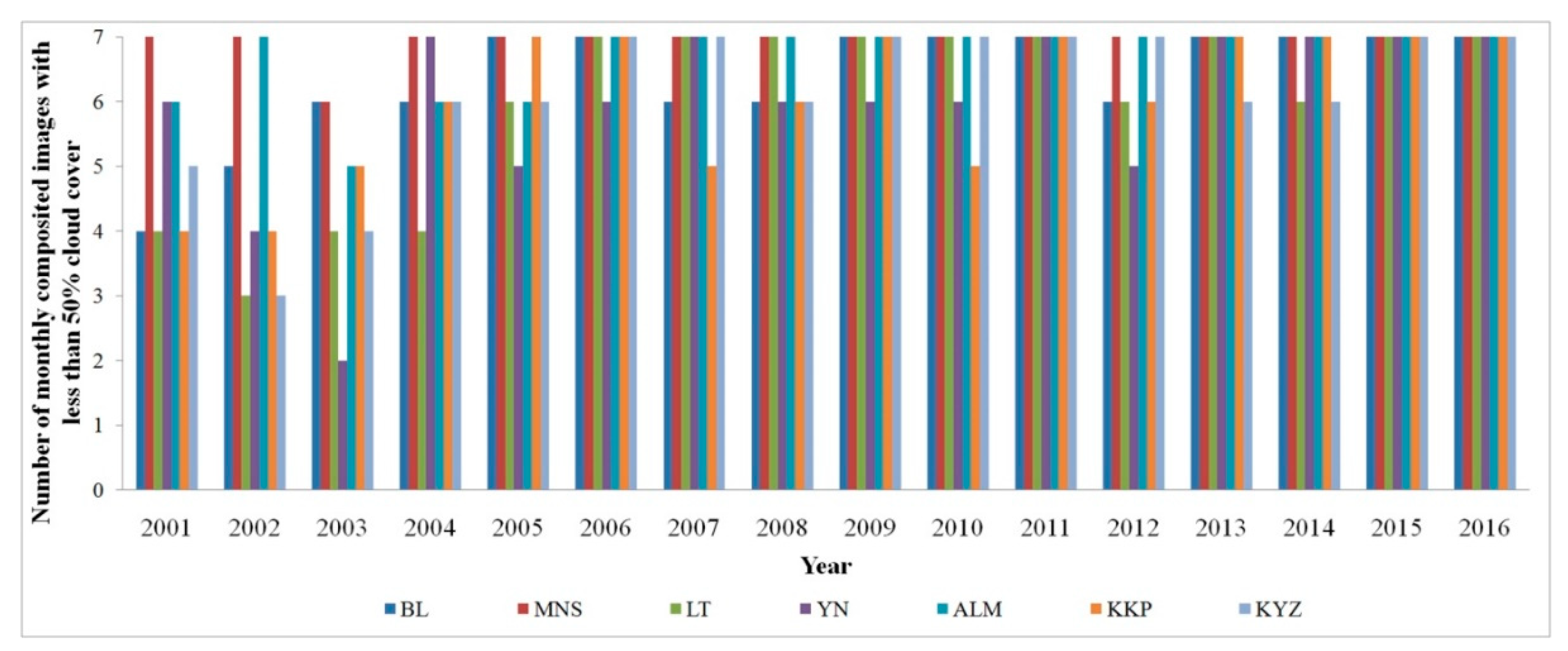
Data availability of each study region. Note: This figure shows the data availability in the seven study regions of this study. After monthly image composition, we acquired the monthly maximum normalized difference vegetation index (NDVI) time series between April and October for each year. Therefore, for each study region, we acquired seven images (one for each month). For each pixel of an image, for example, the April image of BL in 2016, if no cloud-free period is recorded during this month, the pixel was labelled “non value” in the composited 2016 April image. Then we used the number of 50% monthly composited cloud-free periods for each study region/year to represent the data availability in this figure. For example, the 2016 images in BL show that more than 50% cloud-free pixels were acquired in all seven monthly composited images, while for the 2003 images in LT, we acquired only two monthly composited images with more than 50% cloud-free pixels.
Figure 3.
Data availability of each study region. Note: This figure shows the data availability in the seven study regions of this study. After monthly image composition, we acquired the monthly maximum normalized difference vegetation index (NDVI) time series between April and October for each year. Therefore, for each study region, we acquired seven images (one for each month). For each pixel of an image, for example, the April image of BL in 2016, if no cloud-free period is recorded during this month, the pixel was labelled “non value” in the composited 2016 April image. Then we used the number of 50% monthly composited cloud-free periods for each study region/year to represent the data availability in this figure. For example, the 2016 images in BL show that more than 50% cloud-free pixels were acquired in all seven monthly composited images, while for the 2003 images in LT, we acquired only two monthly composited images with more than 50% cloud-free pixels.

Figure 4.
Exemplary training samples and corresponding NDVI signatures from Landsat images. The NDVI color is presented as R: NDVI in September of 2016; G: NDVI in July of 2016; B: NDVI in May of 2016. Note: We collected polygons based on very high resolution (VHR) images and visually interpreted these samples using both Landsat NDVI time series and the VHR image, and finally converted the polygons to Landsat pixels. These samples are pure pixels as they were collected in homogenous regions based on the VHR images.

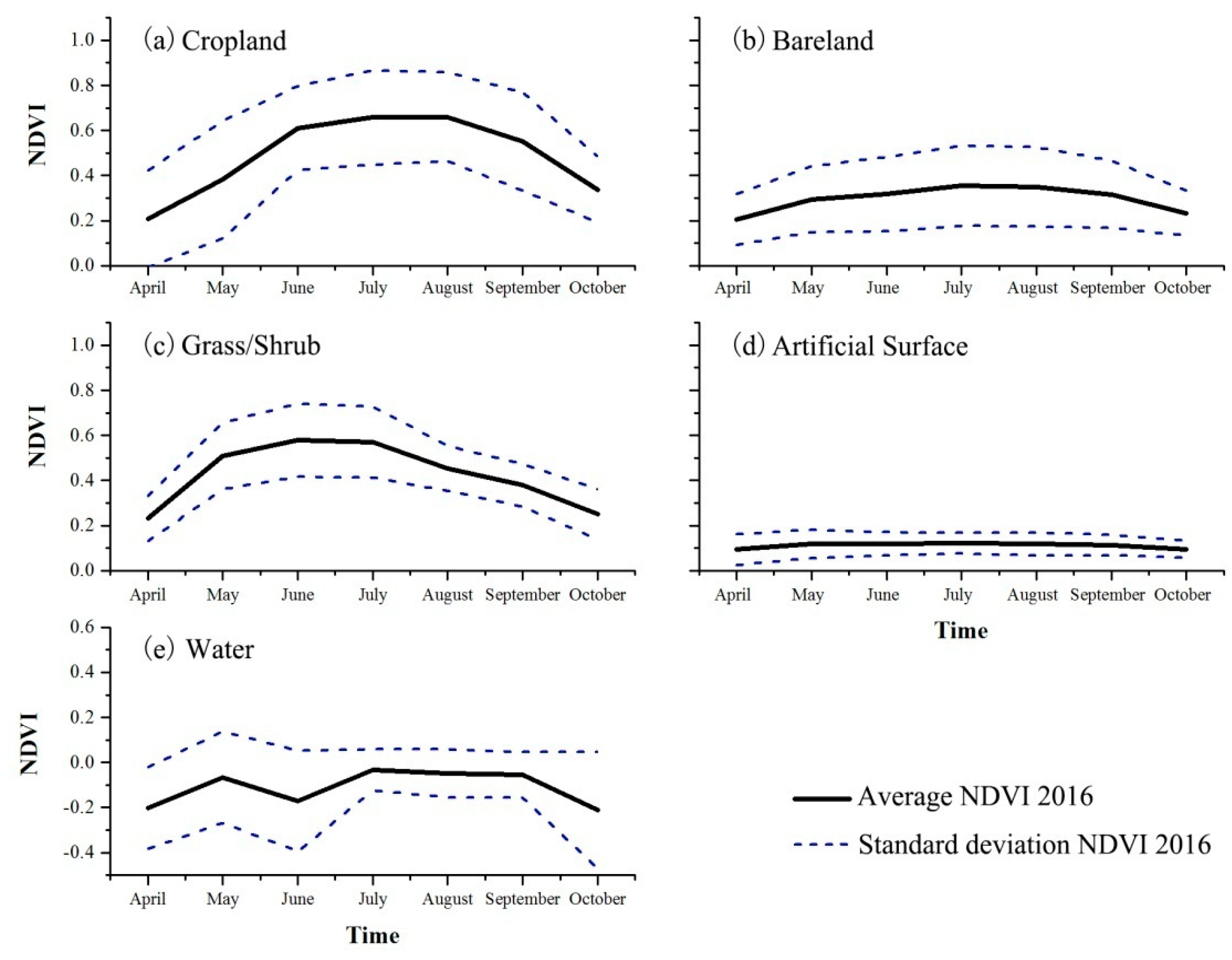
Figure 5.
Average and standard deviation of NDVI time series for each class in 2016. Note: NDVI time series of training samples of all seven study sites were used to generate this figure.
Figure 5.
Average and standard deviation of NDVI time series for each class in 2016. Note: NDVI time series of training samples of all seven study sites were used to generate this figure.

Figure 6.
ABNet model and the procedure of generating reference time series. (a) ABNet model, (b) procedure of generating reference time series. ABNet, Antibody network.
Figure 6.
ABNet model and the procedure of generating reference time series. (a) ABNet model, (b) procedure of generating reference time series. ABNet, Antibody network.

Figure 7.
Procedure of classifying times series with “missing data”.

Figure 8.
Gini importance scores of two optimal features for each study site.

Figure 9.
Classification accuracy of annual classifications in seven test sites. Notes: (a) BL, (b) MNS, (c) LT, (d) YN, (e) KYZ, (f) KKP, (g) ALM, (h) average and standard deviation of classification accuracy among the 16 years.
Figure 9.
Classification accuracy of annual classifications in seven test sites. Notes: (a) BL, (b) MNS, (c) LT, (d) YN, (e) KYZ, (f) KKP, (g) ALM, (h) average and standard deviation of classification accuracy among the 16 years.

Figure 10.
Comparison of the cropland maps in 2010. Note: The images in different study regions have different scale bars in this figure.
Figure 10.
Comparison of the cropland maps in 2010. Note: The images in different study regions have different scale bars in this figure.

Figure 11.
Annual change in cropland area in seven test sites in Central Asia: (a) BL, (b) MNS, (c) LT, (d) YN, (e) KYZ, (f) KKP, (g) ALM. Note: The area of cropland increased in BL, MNS, LT, and YN between 2001 and 2016, and in KKP, KYA and ALM, cropland acreage does not have the increasing trend.
Figure 11.
Annual change in cropland area in seven test sites in Central Asia: (a) BL, (b) MNS, (c) LT, (d) YN, (e) KYZ, (f) KKP, (g) ALM. Note: The area of cropland increased in BL, MNS, LT, and YN between 2001 and 2016, and in KKP, KYA and ALM, cropland acreage does not have the increasing trend.

Figure 12.
Cropland changes and the number of cropped years for each pixel. Note: crop intensity means among the 16 years of this study, the number that a pixel identified as cropland was defined as the cropland intensity (cropped years). In this figure, we show the cropland extent at 2001, 2006, 2011, and 2016 for all study regions, and also show the cropland intensity. In the cropland intensity image, green patterns represent low cropland intensity regions and red patterns represent high cropland intensity regions. Generally, BL, MNS, LT, and YN had higher land use intensity than the other four study regions. In addition, the images of this figure share the same scale bar.


Table 1.
Summary of the seven study areas in Xinjiang and the Aral Sea basin.
| Name of Study Site (Abbreviations) | Bole (BL) | Manas (MNS) | Luntai (LT) | Yining (YN) | Almaty (ALM) | Karakalpakstan (KKP) | Kyzl-Orda (KYZ) |
|---|---|---|---|---|---|---|---|
| Country | China | China | China | China | Kazakhstan | Kazakhstan | Uzbekistan |
| Centre coordinates | 82.54E, 44.52N | 86.50E, 44.54N | 84.51E, 41.53N | 81.13E, 43.89N | 74.72E, 43.48N | 64.39E, 44.99N | 59.18E, 42.98N |
| Elevation (meters above sea level) | 1057.84 | 480.29 | 943.88 | 772.43 | 949.67 | 105.47 | 64.89 |
| Major crops | Cotton | Cotton | Cotton, Maize Wheat | Cotton, Wheat | Wheat, Barley, Cotton | Wheat, Cotton, Alfalfa | Rice, Alfalfa Wheat |
| Length of growing season | April–October | April–October | March–September | April–October | April–October | April–October | April–October |
Table 2.
Features extracted from the Landsat images.
| Band/Vegetation Index | Band Number of the Sensor | Refs | |
|---|---|---|---|
| Median value | 2 (Landsat-8 OLI), 1 (Landsat-7 ETM+ and 5 TM) | ||
| 3 (Landsat-8 OLI), 2 (Landsat-7 ETM+ and 5 TM) | |||
| 4 (Landsat-8 OLI), 3 (Landsat-7 ETM+ and 5 TM) | |||
| 5 (Landsat-8 OLI), 4 (Landsat-7 ETM+ and 5 TM) | |||
| 6 (Landsat-8 OLI), 5 (Landsat-7 ETM+ and 5 TM) | |||
| 7 (Landsat-8 OLI), 7 (Landsat-7 ETM+ and 5 TM) | |||
| Median value | Normalized Difference Vegetation Index (NDVI) | [42] | |
| Normalized Burn Ratio (NBR) | [43] | ||
| Normalized Difference Moisture Index (NDMI) | [44] | ||
| Green Vegetation Index (VIGreen) | [45] | ||
| Normalized Difference Moisture Index (NDSI) | [46] |
Note: indicates multi-spectral band.
Table 3.
Number of training samples (pixels) for different land cover types in seven test sites.
| Class | BL | MNS | LT | YN | ALM | KKP | KYZ |
|---|---|---|---|---|---|---|---|
| Cropland | 3716 | 2968 | 3422 | 1465 | 2153 | 621 | 381 |
| Bareland | 1957 | 843 | 6006 | 273 | 427 | 537 | 1465 |
| Artificial surface | 920 | 511 | 427 | 321 | 273 | 321 | 356 |
| Shrub/Grass | 1660 | 542 | 3012 | 356 | 221 | 1144 | 346 |
| Water | 1628 | 509 | 643 | 221 | 319 | 315 | 205 |
Table 4.
Number of randomly selected validation samples (pixels) between 2001 and 2016 for cropland (C) and non-cropland (N) in seven test sites.
Table 4.
Number of randomly selected validation samples (pixels) between 2001 and 2016 for cropland (C) and non-cropland (N) in seven test sites.
| Year | BL | MNS | LT | YN | ALM | KKP | KYZ | |||||||
|---|---|---|---|---|---|---|---|---|---|---|---|---|---|---|
| C | N | C | N | C | N | C | N | C | N | C | N | C | N | |
| 2001 | 161 | 821 | 356 | 644 | 86 | 914 | 391 | 609 | 115 | 819 | 121 | 879 | 92 | 840 |
| 2002 | 164 | 818 | 350 | 650 | 87 | 913 | 396 | 604 | 169 | 819 | 116 | 884 | 136 | 824 |
| 2003 | 176 | 806 | 369 | 631 | 93 | 907 | 400 | 600 | 147 | 816 | 110 | 890 | 139 | 836 |
| 2004 | 179 | 803 | 381 | 619 | 93 | 907 | 415 | 585 | 169 | 821 | 99 | 901 | 130 | 844 |
| 2005 | 183 | 799 | 389 | 611 | 95 | 905 | 416 | 584 | 168 | 821 | 102 | 898 | 71 | 837 |
| 2006 | 190 | 792 | 396 | 604 | 92 | 902 | 426 | 574 | 167 | 818 | 101 | 899 | 114 | 808 |
| 2007 | 200 | 782 | 400 | 600 | 105 | 895 | 435 | 565 | 152 | 822 | 106 | 894 | 100 | 771 |
| 2008 | 199 | 783 | 411 | 589 | 111 | 889 | 439 | 561 | 147 | 830 | 104 | 896 | 69 | 882 |
| 2009 | 206 | 776 | 419 | 581 | 120 | 880 | 443 | 557 | 150 | 827 | 122 | 878 | 99 | 744 |
| 2010 | 212 | 770 | 430 | 570 | 126 | 874 | 446 | 554 | 207 | 789 | 116 | 884 | 111 | 766 |
| 2011 | 226 | 749 | 450 | 549 | 138 | 862 | 439 | 547 | 157 | 759 | 120 | 880 | 112 | 774 |
| 2012 | 237 | 745 | 456 | 544 | 149 | 851 | 457 | 543 | 205 | 790 | 112 | 888 | 61 | 778 |
| 2013 | 249 | 733 | 471 | 429 | 156 | 844 | 459 | 541 | 188 | 791 | 118 | 881 | 66 | 791 |
| 2014 | 255 | 726 | 484 | 516 | 165 | 835 | 458 | 542 | 196 | 794 | 135 | 865 | 56 | 798 |
| 2015 | 256 | 726 | 487 | 513 | 181 | 819 | 462 | 538 | 208 | 792 | 140 | 860 | 52 | 760 |
| 2016 | 256 | 726 | 492 | 508 | 184 | 816 | 469 | 531 | 202 | 798 | 149 | 851 | 108 | 758 |
Table 5.
Classification accuracy comparison with FROM–GLC and GlobaLand30 in seven study regions.
| Study Site | RBM | FROM–GLC | GlobaLand30 | Study Site | RBM | FROM–GLC | Globaland30 | ||
|---|---|---|---|---|---|---|---|---|---|
| OA(%) | BL | 96.33 | 95.73 | 96.29 | MNS | 92.6 | 81.3 | 88.9 | |
| Kappa | 0.8928 | 0.8798 | 0.8911 | 0.8468 | 0.6202 | 0.8068 | |||
| C | PA(%) | 92.92 | 92.87 | 92.75 | 85.35 | 80 | 85.81 | ||
| UA(%) | 90.37 | 90.45 | 91.67 | 97.09 | 77.3 | 88.79 | |||
| N | PA(%) | 97.27 | 97.11 | 99.04 | 98.07 | 82.28 | 97.54 | ||
| UA(%) | 98.04 | 98.19 | 98.76 | 89.87 | 84.5 | 93.93 | |||
| OA(%) | LT | 97.9 | 91.7 | 95.1 | YN | 95.3 | 72.49 | 92.3 | |
| Kappa | 0.9043 | 0.8272 | 0.7639 | 0.9049 | 0.4363 | 0.8452 | |||
| C | PA(%) | 91.27 | 90.26 | 73.81 | 94.84 | 47.49 | 94.84 | ||
| UA(%) | 92 | 85.93 | 86.32 | 94.63 | 90 | 88.68 | |||
| N | PA(%) | 98.86 | 97.83 | 98.17 | 95.67 | 96.21 | 90.25 | ||
| UA(%) | 98.74 | 98.48 | 96.3 | 95.84 | 66.61 | 95.6 | |||
| OA(%) | KKP | 96 | 78.51 | 91.23 | KYZ | 95.68 | 94.8 | 70.68 | |
| Kappa | 0.8223 | 0.4763 | 0.8028 | 0.8766 | 0.8607 | 0.4143 | |||
| C | PA(%) | 93.97 | 81.64 | 88.28 | 98.07 | 91.39 | 100 | ||
| UA(%) | 76.76 | 48.99 | 75 | 83.88 | 82.81 | 41.48 | |||
| N | PA(%) | 96.27 | 77.69 | 95.7 | 95.06 | 97.51 | 62.99 | ||
| UA(%) | 99.18 | 94.16 | 99.76 | 99.47 | 98.85 | 100 | |||
| OA(%) | ALM | 96.92 | 85.52 | 78.34 | |||||
| Kappa | 0.8674 | 0.5008 | 0.4317 | ||||||
| C | PA(%) | 93.69 | 79.28 | 99.1 | |||||
| UA(%) | 83.87 | 45.83 | 36.79 | ||||||
| N | PA(%) | 97.39 | 86.42 | 75.33 | |||||
| UA(%) | 99.07 | 96.64 | 99.83 | ||||||
Notes: OA = overall accuracy, PA = producer´s accuracy, UA = user´s accuracy. “C” denotes Cropland, “N” denotes Non-Cropland, “RBM” denotes reference-time-series based mapping method.
Table 6.
McNemar’s test result of RBM results and the two existing cropland maps (Z value and significant level).
Table 6.
McNemar’s test result of RBM results and the two existing cropland maps (Z value and significant level).
| BL | MNS | LT | YN | ALM | KKP | KYZ | |
|---|---|---|---|---|---|---|---|
| RBM vs. Globaland30 | 0.94 (N) | −0.14 (N) | 0.75 (N) | 0.93 (N) | 6.22 (S+) | 9.76 (S+) | 0.19 (N) |
| RBM vs. FROM–GLC | −0.29 (N) | 9.41 (S+) | 1.51 (N) | 5.17 (S+) | 1.97 (S+) | 6.64 (S+) | 1.01 (N) |
© 2018 by the authors. Licensee MDPI, Basel, Switzerland. This article is an open access article distributed under the terms and conditions of the Creative Commons Attribution (CC BY) license (http://creativecommons.org/licenses/by/4.0/).
Share and Cite
MDPI and ACS Style
Hao, P.; Löw, F.; Biradar, C. Annual Cropland Mapping Using Reference Landsat Time Series—A Case Study in Central Asia. Remote Sens. 2018, 10, 2057. https://0-doi-org.brum.beds.ac.uk/10.3390/rs10122057
AMA Style
Hao P, Löw F, Biradar C. Annual Cropland Mapping Using Reference Landsat Time Series—A Case Study in Central Asia. Remote Sensing. 2018; 10(12):2057. https://0-doi-org.brum.beds.ac.uk/10.3390/rs10122057
Chicago/Turabian StyleHao, Pengyu, Fabian Löw, and Chandrashekhar Biradar. 2018. "Annual Cropland Mapping Using Reference Landsat Time Series—A Case Study in Central Asia" Remote Sensing 10, no. 12: 2057. https://0-doi-org.brum.beds.ac.uk/10.3390/rs10122057
Note that from the first issue of 2016, this journal uses article numbers instead of page numbers. See further details here.