Letter

Model-Based Optimization of Spectral Sampling for the Retrieval of Crop Variables with the PROSAIL Model

1
Department of Geography, Ludwig-Maximilians-Universität München, Luisenstraße 37, D-80333 Munich, Germany
2
Institute of Surveying, Remote Sensing & Land Information (IVFL), University of Natural Resources and Life Sciences, Vienna (BOKU), Peter Jordan Str. 82, 1190 Vienna, Austria
*
Author to whom correspondence should be addressed.
Remote Sens. 2018, 10(12), 2063; https://0-doi-org.brum.beds.ac.uk/10.3390/rs10122063
Submission received: 19 September 2018 / Revised: 13 December 2018 / Accepted: 17 December 2018 / Published: 19 December 2018
(This article belongs to the Special Issue Applications of Spectroscopy in Agriculture and Vegetation Research)

Abstract

:
Satellite hyperspectral Earth observation missions have strong potential to support sustainable agriculture by providing accurate spatial and temporal information of important vegetation biophysical and biochemical variables. To meet this goal, possible error sources in the modelling approaches should be minimized. Thus, first of all, the capability of a model to reproduce the measured spectral signals has to be tested before applying any retrieval algorithm. For an exemplary demonstration, the coupled PROSPECT-D and SAIL radiative transfer models (PROSAIL) were employed to emulate the setup of future hyperspectral sensors in the visible and near-infrared (VNIR) spectral regions with a 6.5 nm spectral sampling distance. Model uncertainties were determined to subsequently exclude those wavelengths with the highest mean absolute error (MAE) between model simulation and spectral measurement. The largest mismatch could be found in the green visible and red edge regions, which can be explained by complex interactions of several biochemical and structural variables in these spectral domains. For leaf area index (LAI, m2·m−2) retrieval, results indicated only a small improvement when using optimized spectral samplings. However, a significant increase in accuracy for leaf chlorophyll content (LCC, µg·cm−2) estimations could be obtained, with the relative root mean square error (RMSE) decreasing from 26% (full VNIR range) to 15% (optimized VNIR) for maize and from 77% to 29% for soybean, respectively. We therefore recommend applying a specific model-error threshold (MAE of ~0.01) to stabilize the retrieval of crop biochemical variables.

Graphical Abstract

1. Introduction

Worldwide, there is an increasing interest in and need to optimize agricultural management systems to enhance yields while minimizing environmental impacts [1]. Earth observation (EO) supports precision agriculture techniques by providing accurate spatial and temporal information of vegetation biophysical and biochemical variables, such as leaf area index (LAI, in m2·m−2) and leaf chlorophyll content (LCC, in µg·cm−2) [2]. As several satellite hyperspectral EO missions are due to launch, these vegetation quantities will soon be monitored over large areas with potentially higher accuracies than is possible with today’s multispectral systems [3]. Planned missions for the near future include, for instance, the Italian Prototype Research Instruments and Space Mission Technology Advancement (PRISMA) [4] and the US Hyperspectral Infrared Imager (HyspIRI) [5], as well as the two German missions, the DLR Earth Sensing Imaging Spectrometer (DESIS) [6] and the Environmental Mapping and Analysis Program (EnMAP) [7].
The expected global availability of hyperspectral data requires the development of generic and transferable retrieval techniques [8,9]. Considering the high spectral information content that will be provided by the new sensors, physically based retrieval techniques combined with flexible and computationally efficient machine-learning regression algorithms (MLRAs) can strongly support the effective exploitation of the full spectral signals. This can be realized, for instance, by employing radiative transfer models (RTM) such as the well-known and widely used canopy bidirectional reflectance model 4SAIL [10] and the PROSPECT-D leaf optical properties model [11]. The combined model version, commonly called PROSAIL [12], constitutes an ideal compromise between model complexity and computational efficiency, in particular for the efficient processing of large datasets and especially for agricultural crops [13]. To retrieve the sought biophysical or biochemical variable via RTM inversion, most commonly, look-up table (LUT) approaches [14,15,16,17] are applied. Such LUTs store a defined number (e.g., 100,000) of canopy parameter realizations and their corresponding simulated spectral reflectance. LUTs also serve as training databases for MLRAs within hybrid retrieval schemes [8].
Compared to the estimation of structural variables such as LAI, the estimation of biochemical leaf variables from the canopy signals has often been found to be difficult [18,19]. Besides the use of hyperspectral data, the implementation of model constraints can enhance the estimation accuracy of those quantities [20,21]. Useful constraints include, for instance:
  • spectral constraints: limit the analysis to predefined spectral samplings or spectral regions where the variable of interest dominates the spectral signal (e.g., [22]);
  • sampling constraints: predefine the distribution of the variables in the LUT, such as uniform or Gaussian based on a priori information, either from field sites or derived from growth models (e.g., [20,22]);
  • spatial constraints: take neighborhood information into account, resulting in object-based retrieval (e.g., [23]);
  • temporal constraints: use temporal autocorrelation to modify the cost function (e.g., [17,20]).
Such constraints, however, can only support accurate product retrieval if the prerequisite of having error-free measurements and model simulations is fulfilled. Indeed, a drawback of the physically based approaches—especially in the context of hyperspectral data—is associated to their sensitivity to corrupted or less well-modelled (and measured) wavelengths, biasing the retrieval [24,25]. This implies the need to test the models’ capability of reproducing the reflectance signal of the vegetation of interest before applying RTMs for the retrieval of biophysical and biochemical variables. Even small discrepancies between modelled and measured reflectance may otherwise affect the final retrieval accuracy. In a study by Atzberger et al. [24], this was exemplified for grasslands. Using a fully automated feature-selection (FS) algorithm, poorly modelled wavebands were sequentially identified and discarded, leading to more accurate variable estimations. A study analyzing different crops and a multispectral dataset [23] had to discard three from six crops (including maize) since the forward modelling, parameterized by field-measured LAI, did not match the observed signatures. The mismatch led to a failure of the LUT-based inversion. The future availability of hyperspectral data will allow for the more specific identification of modelled and measured spectral uncertainties. Feature-selection algorithms, as proposed by Atzberger et al. [24], can be implemented to improve retrieval. In view of the complex and varying canopy structures, such tests should be repeated on various crop types at different sites and with actual sensors throughout the growing season.
In this context, the objective of the present study was to test the capability of the PROSAIL model to reproduce hyperspectral measurements in the visible to near infrared (VNIR) region and to analyze the impact of erroneous bands—and their subsequent removal—on the retrieval of LAI and LCC for agricultural crops. We thus aim to improve the usability of PROSAIL simulations for two important crop types (maize and soybean) as a prerequisite for the application of the model within a retrieval scheme for biophysical and biochemical variables from future hyperspectral sensor missions’ data.

2. Materials and Methods

2.1. Data Collection and Preparation

Spectroscopic data were collected concurrently with biophysical and biochemical variables at the University of Nebraska–Lincoln Agricultural Research and Development Center (UNL-ARDC), which takes part in the Carbon Sequestration Program. Spectroscopic measurements in the 400–1000 nm domain were carried out during multiple years at three agricultural fields (irrigated maize and irrigated maize–soybean rotation at 41°09′54.2″N, 96°28′35.9″W, 361 m above sea level (a.s.l.); and rain-fed maize–soybean rotation at 41°10′46.8″N, 96°26′22.7″W, 362 m a.s.l.) using a dual-fiber optics system (i.e., two Ocean Optics USB2000 radiometers) mounted on an all-terrain sensor platform. Spectral reflectance sampling areas were associated to intensive measurement zones (IMZ). At each IMZ, green leaf area index (LAI, m2·m−2) and leaf chlorophyll content (LCC, µg·cm−2) measurements were carried out destructively from June 2001 to August 2008 [26,27]. Since a spectral sampling distance of 6.5 nm represents a good compromise between several upcoming hyperspectral sensors, ranging from 2.55 nm (DESIS) over 6.5 nm (EnMAP) to 12 nm (PRISMA), EnMAP band-specific spectral response functions with 6.5 nm spectral sampling distance were applied to the field spectrometer data in the VNIR domain (Nsamples = 73 bands in the spectral range 423–863 nm). Due to the presence of noise in the spectrometer data above 870 nm, we decided to exclude the central wavebands from 871 nm to 975 nm. In this way, the available spectral information is reduced while still providing a valid hyperspectral database for the exploitation of optimal LAI and LCC retrieval. Currently, there are no spaceborne sensors and only very few airborne sensors that are suitable to ‘emulate’ the future satellites with the appropriate spectral resolution, signal-to-noise ratio (SNR) and sampling (especially the temporal sampling to cover different phenological phases), with field sampling activities running in parallel. Although there may be some spectral information missing, a field spectroscopy database is still ideal to simulate VNIR bands from future hyperspectral spaceborne sensors.
Note that the converted measurements were assumed to be error-free. However, the inclusion of measurement uncertainties in the inversion process may lead to improved retrieval, for instance, when using Bayesian techniques [28]. Moreover, spatial resolution and atmospheric correction issues go beyond the scope of the current study.
For the present study, 169 measurements of LAI (m2·m−2) and LCC (µg·cm−2) were available for maize and 68 samples for soybean. A summary of the variable distribution is presented in Table 1.

2.2. Spectral Feature Selection

From each crop type, 20 sample spectra (corresponding to 20 IMZs) were selected to assess the agreement between the model-simulated and measured spectra and to identify/eliminate poorly simulated spectral bands. The 20-sample spectra were extracted from different dates to represent the range of phenological stages that occur during the course of a growth cycle. Following the procedure outlined in Atzberger et al. [24], for each IMZ, an individual look-up table (LUTind) was established with the PROSAIL model. LAI was fixed at its measured value, while all other model parameters were allowed to vary freely within a uniform distribution. This decision is based on the dominant influence of canopy structure (i.e., LAI) on the overall spectral signal. Soil reflectance and measurement geometry were specified according to actual conditions. Table 2 gives an overview of the specific individual LUT parameterization (LUTind).
For each LUTind, spectral signals were simulated for 10,000 randomly selected parameter combinations. Simulated PROSAIL reflectance values were converted to VNIR bands (Nbands = 73) by applying the actual band-specific response functions of the future EnMAP hyperspectral imager. Due to the narrow spectral range of the field spectrometer used, the simulation was limited to the VNIR part of the spectrum. By means of the root mean square error (RMSE), calculated across the 73 selected bands, the best-fitting LUT spectrum was selected. The mean absolute error (MAE) was calculated for each of the 20 individual IMZs by subtracting the best-fitting LUT spectrum from the corresponding measured spectrum. After calculating the mean value of the resulting 20 MAEs, the least accurately modeled band was deleted and the procedure was repeated, running the LUTind from Nsamples = 73 bands to Nsamples = 1 band. The resulting band combinations were applied to retrieve LAI (in m2·m−2) and LCC (in µg·cm−2) from the validation dataset (i.e., N = 169 for maize and N = 68 for soybean).
To demonstrate the influence of the different parameters on the output reflectance in the analyzed wavelength range (400–865 nm), a global sensitivity analysis (GSA) was carried out. A GSA informs about the contribution of each input parameter to the total variability of the output signal. It further provides information about parameter interactions [32,33]. The GSA was performed for PROSAIL with input parameter ranges as presented in Table 2. A Matlab software tool (GSAT) [34] was applied for this purpose, including both Fourier amplitude sensitivity testing (FAST) analysis and Sobol’s method to calculate first-order sensitivity coefficients. For more details, see also the work of Wang et al. [33].

2.3. Constrained LUT Inversion

For the LUT-based inversion of the PROSAIL model, we followed standard approaches, e.g., [19,30]. The input parameters of the coupled leaf (PROSPECT-D) and canopy reflectance model (SAIL) are displayed in Table 2. Sun zenith angle (SZA) was set to 30°. For the background soil reflectance (ρsoil), the means of different bare soil spectra were calculated and implemented in the model. For leaf chlorophyll content estimations, different constraints were tested to improve the estimates. This included the Gaussian sampling of LCC in the LUT according to current growth stages (maize: mean value (µ) of 50 µg·cm−2, standard deviation (σ) of 20 µg·cm−2; soybean: µ = 30 µg·cm−2 and σ = 20 µg·cm−2). Such information is not commonly available, but in our case, weekly acquisitions could be used to delimit the variables in the LUT according to realistic actual values. Other parameter ranges were set according to Table 2, following uniform distributions. The total size of the LUT was set to 20,000 combinations of input parameters (members) and the corresponding bidirectional reflectance was calculated with the PROSAIL model applying the EnMAP spectral response functions. To select the solution for the inverse problem of a defined measured spectrum, the RMSE between the measured and modeled spectra was calculated, and the best-fitting 50 spectra were selected as the final solution. We chose the best-fitting 50 spectra following the results of Danner et al. [35], who found that the median of the 50 (and 100) best fits—using a RMSE cost function—led to the lowest relative RMSE (rRMSE) for LAI retrieval. According to a study of Darvishzadeh et al. [19], no significant difference was found between the uses of the two statistical parameters of the median and mean. Therefore, we decided to use the mean value, as applied in our previous studies, e.g., [30].

3. Results and Discussion

3.1. Model Suitability Test and Feature Selection

Figure 1 shows the spectral deviations (i.e., MAE) of 20 IMZs between measured and simulated canopy spectra for maize and soybean for known (field-measured) LAI (in m2·m−2).
For both crops, less-accurately modelled bands (i.e., with systematic bias) are situated in the spectral regions between 500 nm and 600 nm and between 700 nm and 800 nm. For maize, we generally observe larger and more frequent discrepancies than for soybean. For instance, the spectral domain from 600 nm to 650 nm was much better simulated for soybean than for maize crops. The similar pattern in Figure 1a,b indicates that PROSAIL has general difficulties in simulating certain spectral regions independent from the crop type. This has also been confirmed by other studies, for instance, analyzing grassland with the PROSAIL model [19] where a similar pattern for the 500–600 nm region was identified. Thus, a more in-depth analysis of the phenomenon is required here: a global sensitivity analysis from the PROSAIL model is used to demonstrate the effects of the different input parameters for each wavelength region (Figure 2).
It becomes clearly evident that exactly in the less well-modelled wavelength range between 500 and 550 nm (green visible (VIS) region), the two pigments of carotenoids (Ccx) and anthocyanins (CAnth) gain influence besides LCC. The total contribution of carotenoids is even stronger than that of chlorophyll content. Obviously, this is the critical wavelength region in which to decouple the effects of these pigments. Moreover, leaf dry matter content (Cm) and the structural SAIL parameters LAI and average leaf inclination angle (ALIA) as well as the soil background contribute to the reflectance signal between 500 nm and 550 nm (Figure 2). Whereas LAI has a quasi-continuous (and largest) influence along the spectral domains, the contribution of ALIA becomes more enhanced from 700 nm onwards. In the so-called red edge region, usually situated between 680–740 nm of the vegetation spectrum, there are also two pronounced peaks of LCC with abrupt leaf reflectance changes. This is caused by the combined effects of strong LCC absorption and leaf internal scattering [36]. The high volatility of parameter contributions in these two spectral regions (green VIS and red edge) may lead to biased reflectance simulations if no proper parameterization has been applied. The question here is whether the leaf optical or the structural canopy model is responsible for the errors: The PROSPECT-D model was largely improved in comparison to its previous versions. This was emphasized by the results shown in the corresponding paper [11], indicating a high accordance of simulated versus measured leaf spectral reflectance (although this analysis was mainly carried out for tree species). Since the signal of the structural canopy parameters is dominant, the SAIL model or its parameterization may play a larger role in the error identification. The interested reader is referred to the paper of Danner et al. [37], in preparation, which discusses the special role of ALIA within the PROSAIL model environment. In summary, the combined effects of all these parameters may explain the discrepancies between simulated and measured reflectance in the two waveband regions: to obtain an optimal model result, input parameters should be defined according to thoroughly measured field data of all required parameters, which is a difficult task rarely accomplished.
On the other hand, we also observe subtle differences between the crop types. This phenomenon can be attributed to crop-specific reflectance behavior, also changing throughout the growing season. The rather simple parameterization of PROSAIL may not be sufficient to describe these canopy structure changes correctly [38]. The study of Atzberger and Richter [23] discarded three from six crop types, amongst them maize, from their analyses as the forward modelling did not match the observed signatures. The authors explained this as a result of the strong row effects not taken into account by the 1D turbid medium model SAIL. Similar findings and explanations were revealed by other studies analyzing maize [30], but in their work, the authors also assumed that the early growth stage with a high (heterogeneous) soil fraction observable by the sensor caused the lower LAI retrieval accuracies compared to sugar beet crops.
The results of the feature-selection experiment are summarized in Figure 3. Initially, the mean absolute error of the simulated versus observed spectral profiles decreases strongly parallel to the decreasing number of bands; see Figure 3a. This effect is observed for maize at a higher level (max MAE = 0.0108) than for soybean reflectance (max MAE = 0.0103). Interestingly, the curves of both crops converge at a certain point (MAE = 0.009) and then decrease linearly until MAE = 0. Applying the corresponding band combinations for variable retrieval, the patterns shown for LAI in Figure 3b and LCC in Figure 3c are obtained. In the case of LAI retrieval, the RMSE of maize increases strongly until band combination 68 is reached—similar to the course of the MAE in the band removal procedure, as illustrated in Figure 3a. From this point onwards, the removal of more bands increases the estimation accuracy until a minimum RMSE of 0.54 m2·m−2 (rRMSE = 0.14) is reached with 42 from 73 spectral bands; 31 bands (mostly in the spectral regions of 500–600 nm and 700–800 nm) were deleted to obtain the optimal accuracy. In the case of soybean LAI, the minimum RMSE of 0.55 m2·m−2 (rRMSE = 0.21) is already reached with 67 from 73 spectral bands. The algorithm deleted only the six least well-simulated bands in the 550 nm and 700 nm regions. For both crops, the further removal of bands (i.e., Nbands < 42/67) again led to an increase in RMSE, indicating that more and more informative bands are removed. The trends for LCC retrieval, demonstrated in Figure 3c, are different: the deletion of the least well-performing bands leads to a very strong increase of retrieval accuracy. After reaching the optimum feature set, accuracy remains stable (soybean) or again slightly decreases (maize). Note that the minimum RMSE occurs at different spectral samplings for each crop and variable type. Hence, an independent generalization can only be achieved through a compromise threshold, where the spectral match is appropriate and at the same time, the retrieval performance of the estimated variables is satisfactory. Looking at Figure 3a–c, this would be the case at around spectral band sampling Nbands ~62, with a mean absolute error in the VNIR domain smaller than 0.01. In the study by Atzberger et al. [24], a threshold of MAE ≤ 0.02 was proposed. However, this finding was based on the full spectrum (HyMap sensor) with the short-wave infrared (SWIR) domain exhibiting the highest inaccuracies between the simulated and measured reflectance. Note that our study provides results from the VNIR region only, which includes the absorption spectra of leaf pigments (e.g., LCC) and the NIR shoulder that is very sensitive to canopy structure effects (i.e., LAI).

3.2. Biophysical and Biochemical Variable Estimations

For LAI, an estimation accuracy of RMSE = 0.55 m2·m−2 was obtained for maize using all available VNIR bands (Nbands = 73). Applying the model-based optimized spectral sampling (Nbands = 42) resulted in no significant retrieval improvement with RMSE = 0.54 m2·m−2. For soybean LAI, similar results were obtained with RMSE = 0.57 m2·m−2 using Nbands = 73 and RMSE = 0.56 m2·m−2 using optimized sampling (Nbands = 67). Figure 3b indicates both RMSE minima in the respective spectral sampling as explained in Section 3.1.
Generally, the LAI retrieval results are consistent or slightly worse compared to similar studies with relative RMSEs from 0.13 to 0.23 m2·m−2 [35,39,40]. The application of the ‘optimized sampling’ only led to a small and nonsignificant improvement compared to the usage of all available bands (maximal rRMSE difference = 0.01). This is due to the fact that the estimation performance does decrease somewhat after deleting a certain number of bands, especially for soybean; see Figure 3b. The ‘reduced’ spectral information of the Nebraska dataset from 423–863 nm provides valuable information of LAI. An interesting study was conducted by Verrelst et al. [29], who used the same dataset and selected the most important spectral bands for LAI retrieval (406 nm, 746 nm, 792 nm, 794 nm, 798 nm, 858 nm, and 878 nm). The authors also obtained a very high estimation performance for LAI retrieval of RMSE = 0.4, suggesting that this limited spectral range turned out to be sufficient for good retrieval. However, the authors [29] used a very different approach, which was based on the target variable, whereas in our study, the feature selection was purely based on the model itself. A band selection study is highly relevant even if restricted to the VNIR domain. The SWIR region, nonetheless, is a very important spectral region for LAI retrieval as well, as it was demonstrated by global sensitivity analysis of the PROSAIL model (for instance, in [29]), and should certainly be regarded in another study where corresponding spectral data are available—especially if the focus is on leaf water and/or protein content.
However, LAI shows high sensitivity across the whole spectrum (400–2500 nm). It is therefore possible to obtain stable estimates using only a reduced number of wavebands. This has been shown by numerous studies in the last years, for instance [41,42,43], even estimating LAI successfully from multispectral information and/or using simple vegetation indices.
Contrary to LAI, the feature selection showed a significant positive impact for leaf chlorophyll content estimation. This was already evident in Figure 3c, and becomes more obvious in Figure 4: whereas the use of all available VNIR (Nbands = 73) spectral bands led to an overestimation and saturation of the LCC retrieval of maize (see Figure 4a), the exclusion of the seven bands with the highest MAE between the model simulation and spectral measurements (i.e., 705 nm, 712 nm, 719 nm, 726 nm, 733 nm, 740 nm and 748 nm) clearly improved the estimation results, from rRMSE of 0.26 to 0.15 (see Figure 4b).
For soybean, again, a strong LCC overestimation prevails when using all available 73 bands (Figure 4c). When optimizing to Nbands = 53, i.e., excluding 498 nm, 503 nm, 508 nm, 513 nm, 518 nm, 523 nm, 528 nm, 533 nm, 538 nm, 543 nm, 548 nm, 553 nm, 698 nm, 705 nm, 712 nm, 719 nm, 726 nm, 733 nm, 740 nm, and 748 nm central wavelengths, retrieval results significantly improved (see Figure 4d). In summary, results of LCC (µg·cm−2) retrieval clearly show a positive impact of removing spectral bands with absolute MAE (between simulation and measurement) larger than 0.01 before applying the RTM inversion.
The removed wavebands are situated partly in the same spectral region for both crops (red edge from 700–750 nm), where the chlorophyll content has expiring absorption features: In PROSPECT-D, the absorbance of LCC drops below 0.001 beyond 733 nm (0.14% of the maximum factor) and becomes 0 at 781 nm. Moreover, although there is no influence of LCC anymore, the wavebands in the near-infrared (NIR) region from 755 to 863 nm were kept for further simulations. Two factors need to be considered: First, the NIR region can still influence the LCC, as it was also found and explained by, e.g., the study of Verrelst et al. [29]. They selected the following nine bands for optimal LCC retrieval: 482 nm, 500 nm, 564 nm, 710 nm, 712 nm, 714 nm, 878 nm, 966 nm, and 980 nm. The authors explained this phenomenon by mechanisms of variable covariation: measured leaf and canopy variables of the same target hold some dependency as vegetation variables are interrelated. Second, as the reflectance in the VIS region is controlled by both LCC and LAI, it certainly helps to get a good estimation of LAI (from VNIR) to model LCC well. Here, the NIR region is used somehow to ‘normalize’ for variations in biomass/LAI. For soybean, even wavelengths from the chlorophyll-sensitive region had to be removed (green visible range 500–550 nm). In the study of Verrelst et al. [29], the red edge region was found to be important for LCC retrieval using the same dataset, but when applying a statistical feature-selection method (based on Gaussian processes regression, GPR), which was directly applied on the target in situ validation dataset. However, in our study, the feature selection was purely model-based, implying that the selected spectral samplings only relied on spectral fits between the model simulation and reflectance measurements before the retrieval algorithm was applied. Therefore, the in situ measured variables had no impact on the retrieval, and a high MAE leads to the exclusion of that band regardless of whether it is sensitive for the variable. Besides, the usage of spectral bands not located in sensitive regions of the considered variable (e.g., the near-infrared region for chlorophyll content) could potentially add some value to the retrieval due to the mechanisms of variable covariation [29]. We could only partly confirm this with our findings, since the red edge region was removed due to PROSAIL simulation failure. The different findings (i.e., different optimal spectral samplings) of our study compared to the study of Verrelst et al. [29] imply that results further depend on the used retrieval algorithm. Statistical methods may achieve the same or even superior variable estimation results with a lower number of bands, but they always rely on the availability of in situ measured variables. This shortcoming can be overcome with a physically based approach. However, the aim of this model error analysis was not to generate the best possible spectral sampling for retrieval of certain variables, but mainly to assure that the simulated reflectance corresponds well with the measured (field/satellite) spectra. Thus, our feature-selection algorithm could be applied at first, and then—if the user has confirmed that the model reproduces the measured spectral bands with satisfying accuracy (for instance, MAE < 0.01)—statistical methods such as a principal component analysis (PCA) could be employed to condense the significant information content, which should further improve the retrieval of the variables. The two approaches therefore have different purposes and effects. With our analysis, we aim to raise the awareness of researchers to the limitations of the applied models.
Even after feature selection, the scatter around the 1:1 line remains high, with rRMSE of 0.15 (maize) and 0.29 (soybean). These values are comparable with other studies, for instance, with rRMSE of 19% and RMSE of 8.4 µg·cm−2 for LCC of the same crops and site [29]. Innovative multispectral EO systems, such as the ESA’s Sentinel-2 sensors, enable the derivation of vegetation products, as shown by many studies (for a discussion, see [3]). However, hyperspectral sensors equipped with very narrow spectral bands over a continuous spectral range will support the detection of vegetation properties more accurately [3]. This may concern, in particular, diverse biochemical plant components, such as chlorophyll, anthocyanins, and carotenoids, with very close and partly overlaying absorption features not distinguishable by broadband scanners. This advantage of hyperspectral over multispectral data was also found by other studies using hyperspectral field data for LCC as well as for LAI estimations [44,45,46]. Whatever the system used, full uncertainty information should be provided along with the biochemical and biophysical products [47], since even small margins of increased accuracy may significantly reduce uncertainties in an operational processing chain [3].

4. Conclusions

Radiative transfer models, such as PROSAIL, have been applied for variable retrieval without testing the model in the forward direction. Researchers often relied on the apparently good experience of previous studies. However, observed spectral reflectance (from field/airborne/spaceborne sensors) can deviate from the forward model simulation in certain spectral regions, further leading to errors in the retrieval with whatever method used. Thus, before inverting these models, suitability tests are recommended [13,24,48]. This implies a need to analyze the model’s capability of reproducing the measured (canopy bidirectional) spectral signals when parameterized using field measurements. Spectral bands with a systematic mismatch between measured and simulated spectra should be removed to avoid bias effects leading to suboptimal performances. So far, no publication exists analyzing the capability of PROSAIL to reproduce crop hyperspectral measurements from simulated data of future sensors, such as HyspIRI, DESIS, PRISMA, or EnMAP. We could show with our analyses that the PROSAIL model is not able to reproduce the measured spectral signals with adequate precision in certain wavelength regions (green VIS/red edge). We could further show that these model limitations depend on the crop type. Eliminating these spectral regions by applying a LUT-based feature-selection algorithm, i.e., deleting the wavebands with MAE > 0.01 between the simulated and measured reflectance, improved variable retrieval (depending on the analyzed crop type and the considered variable). This process can be fully automated and thus could be integrated in standard retrieval schemes, which are based on the comparison of modeled and measured reflectance signatures. Note that these findings are not related to the sensitivity of the variable, but rather to the limited model performance in the green visible and red edge spectral regions for these two specific crop types. Depending on the current growth stage and specific canopy architecture, the simulations can represent the actual measurements with varying precision [13]. It must be taken into consideration, however, that also the collected field spectra may contain errors. To minimize impacts of erroneous field measurements, we analyzed data from 40 experiments with carefully measured spectra.
In summary, our study has two main outcomes:
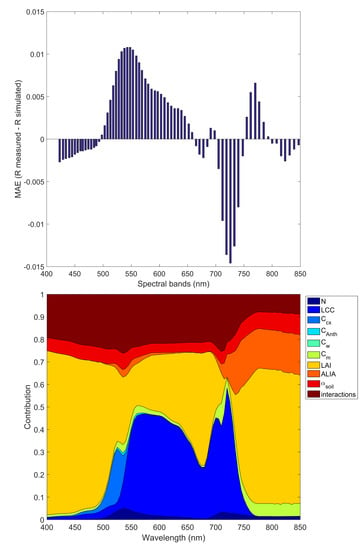
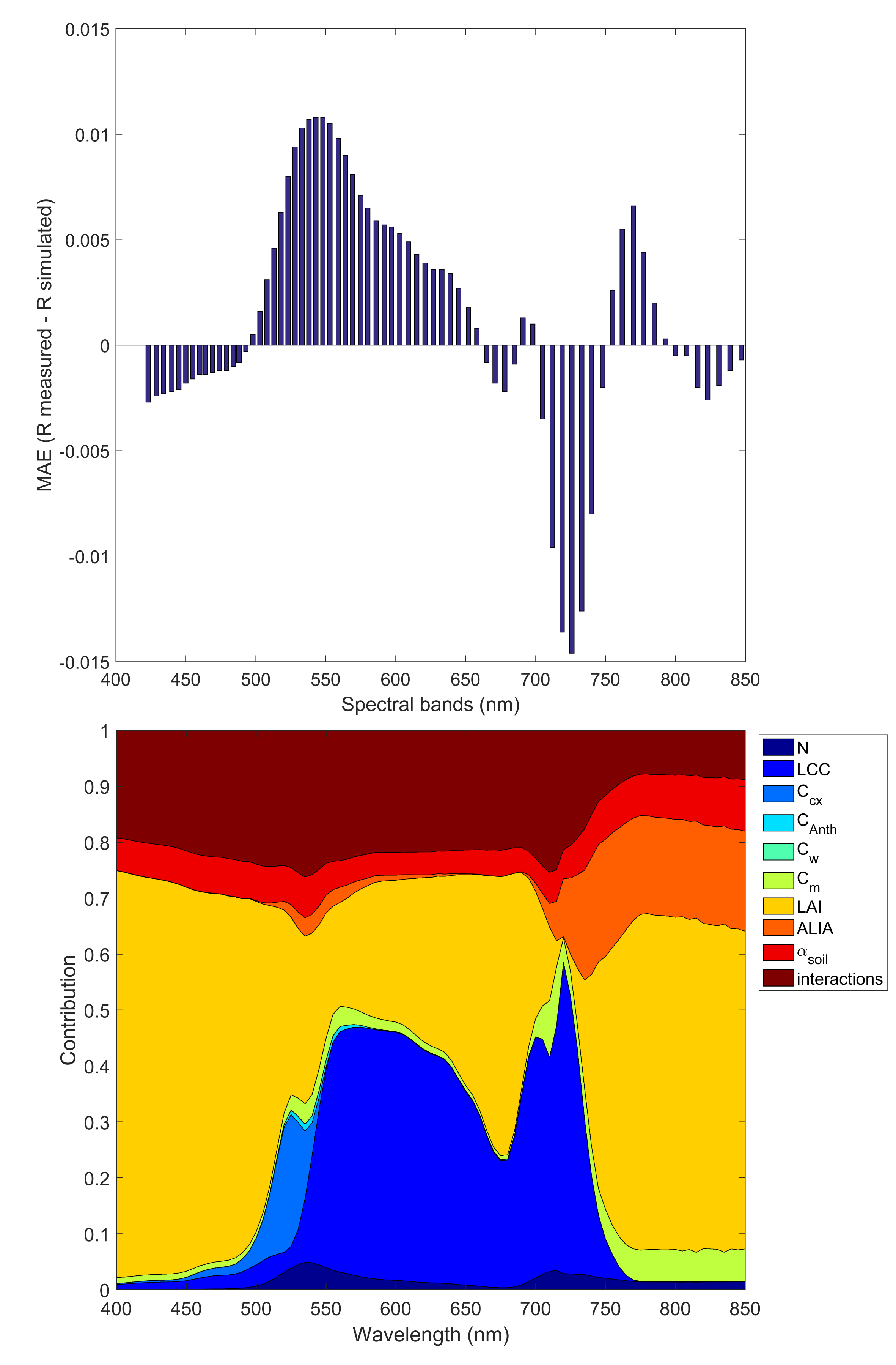
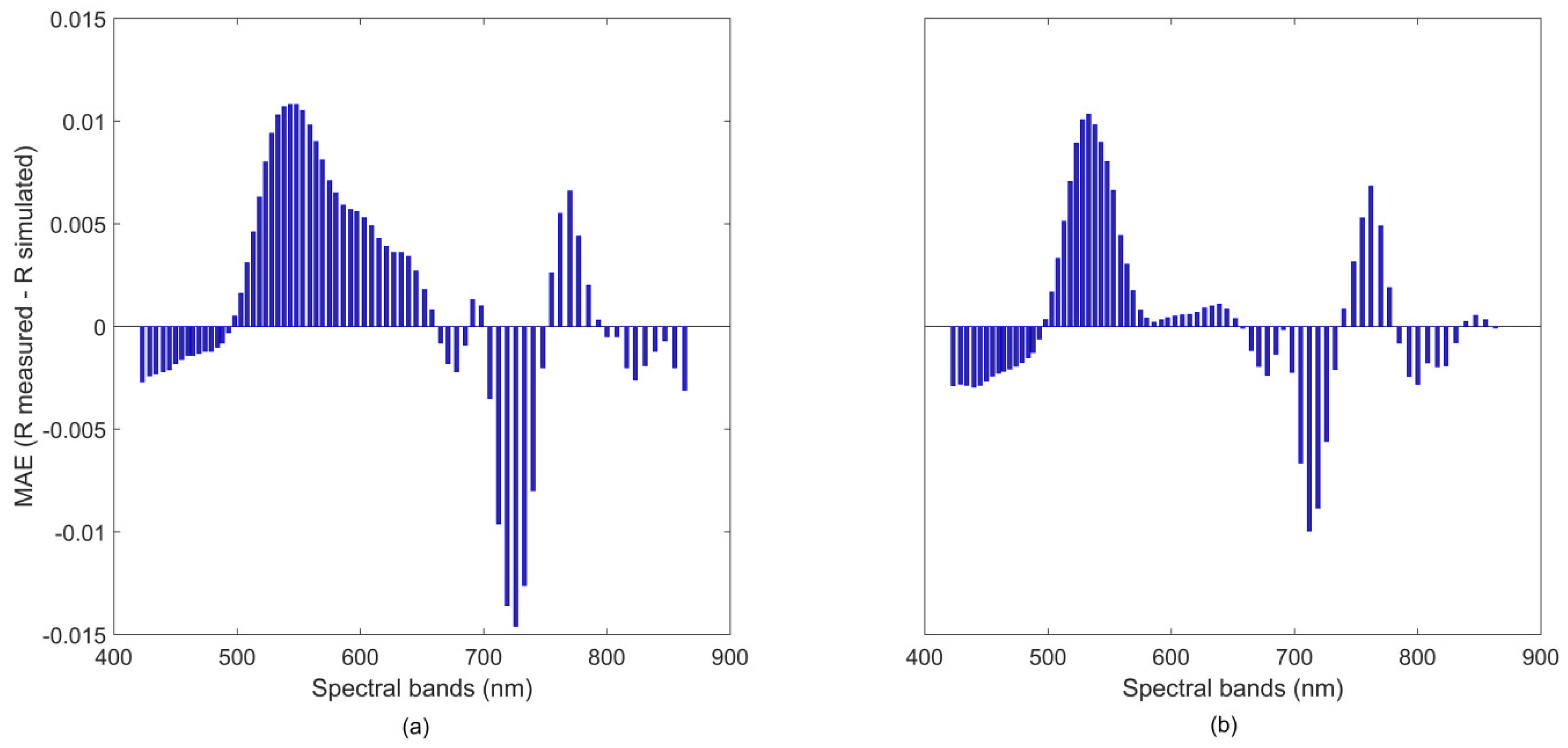
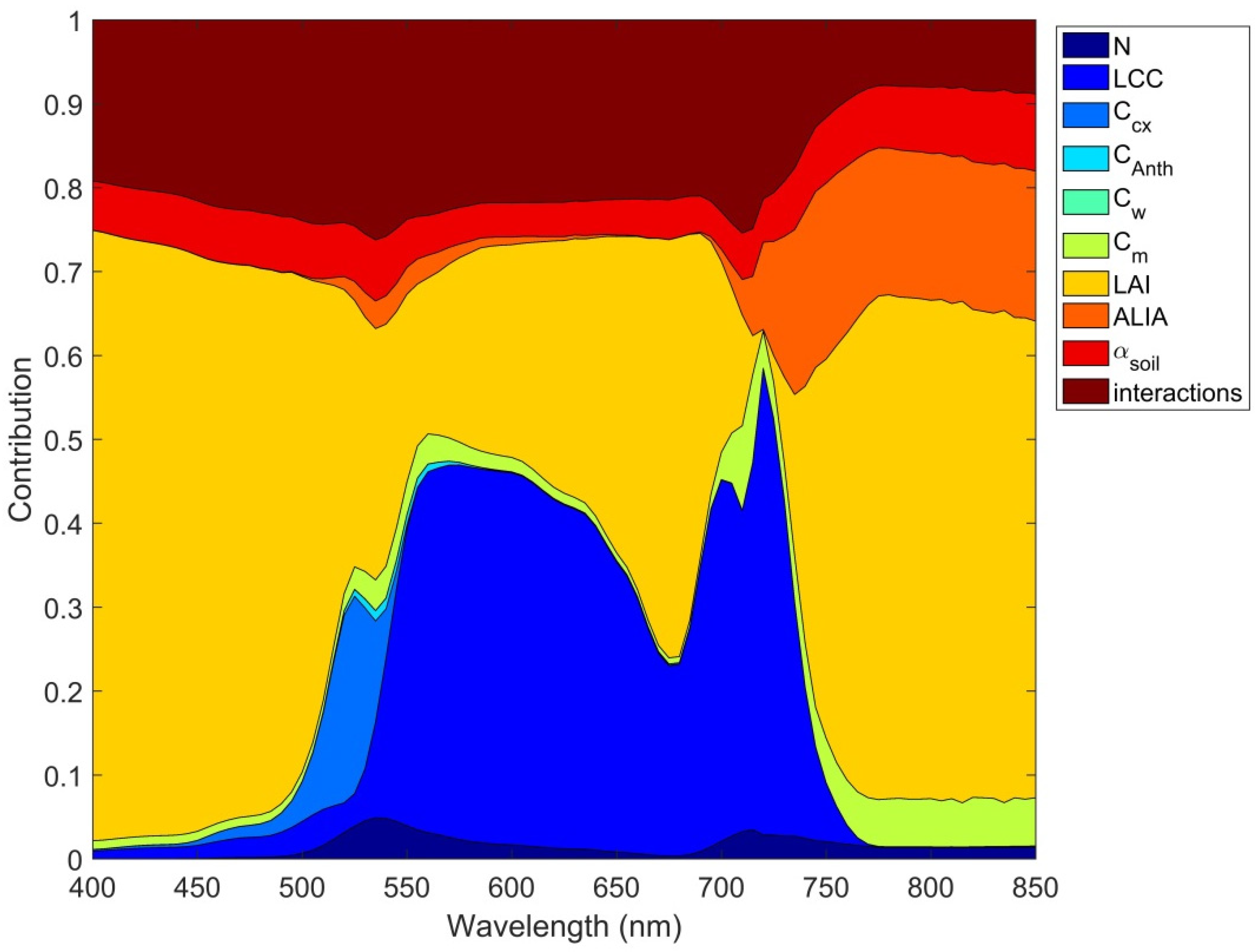
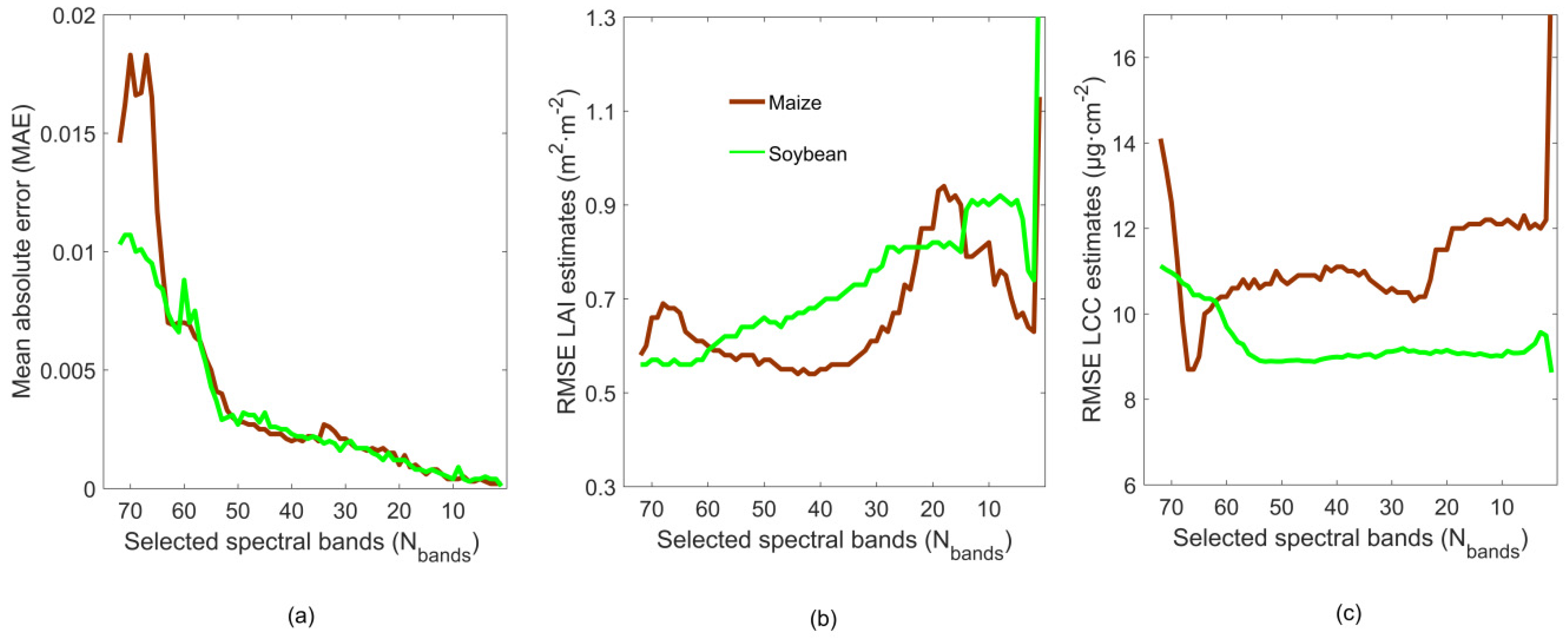
  • There are two spectral regions in the VNIR region which are less well-modelled by PROSAIL independently of crop type: the green visible and the red edge. This can be explained by complex interactions of several biochemical and structural variables in these specific spectral regions. The green visible wavelength region is characterized by the influence of several pigments, in particular, carotenoids, chlorophylls, and anthocyanins. Moreover, there is an influence of leaf dry matter content, LAI, ALIA, and soil background. Regarding the red edge region, there is also a high variability with two strong peaks of chlorophyll content interacting with structural LAI and ALIA parameters.
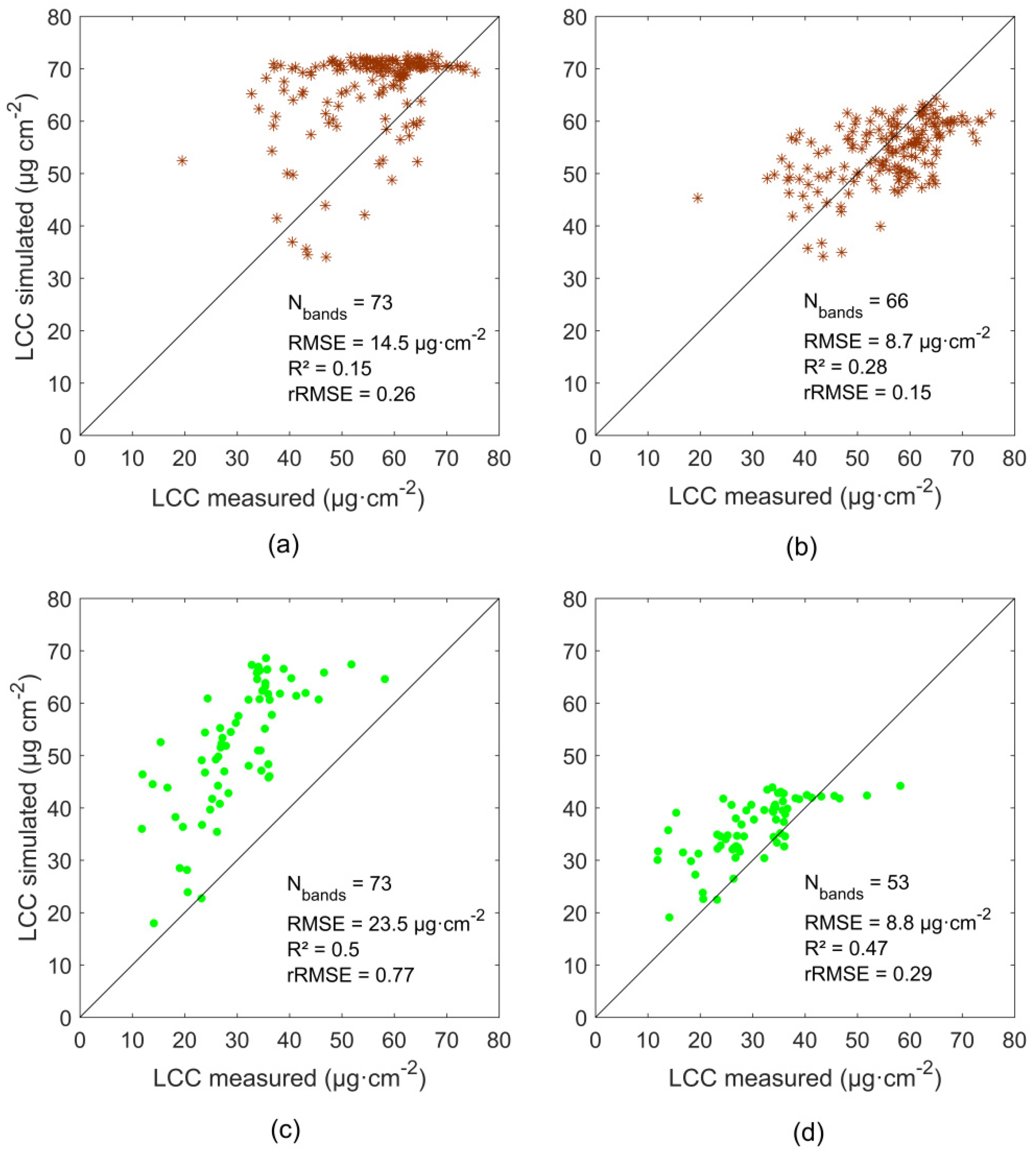
  • Discarding those wavelengths with a spectral mismatch of MAE > 0.01 leads to improvements of the leaf chlorophyll content retrieval. Such model-based analysis should therefore be carried out before applying any retrieval or data reduction algorithm.
The PROSPECT-D model used for this study has been improved using large validation datasets and outperforms previous model versions [11]. However, another prerequisite of a well-working model is proper parameterization. This may even more significantly concern the structural properties of the SAIL model, especially LAI and ALIA. An extensive study is currently in preparation analyzing the suitability of the ALIA parameter within the PROSAIL model environment ([37], intended for the same Special Issue). The practical implications of our results for users of the PROSAIL model would be to parameterize as solidly as possible, optimally through the acquisition of field measurements.
Since for each crop type, specific band combinations were identified, crop-type maps are crucial for the success of our proposed feature-selection method. Alternatively, trade-offs must be defined. For instance, the proposed model-error threshold of MAE ~0.01, at which the model (PROSAIL) matches the measured spectra in the VNIR region for all crops, should be applied before employing any retrieval algorithm in the case that the crop types are not known.
Upcoming spaceborne imaging spectrometers will lead to vast hyperspectral data streams. This calls for automated and optimized spectral uncertainty reduction techniques to ensure fast and efficient data processing, for instance, for the retrieval of vegetation properties. Conclusively, our proposed feature-selection method can provide an efficient measure to improve radiative transfer model simulations that are to be used within retrieval schemes for biophysical and biochemical variables from future hyperspectral sensor missions. To confirm our findings, we strongly recommend extending the study to other crop types as well as other (ground, airborne, and satellite-based) datasets.

Author Contributions

K.B. elaborated the concept, performed the analysis, and wrote most of the manuscript. C.A. helped with interpretation of the findings and writing of the manuscript. M.W. added issues regarding the field campaigns’ data and modelling. M.D. supported in discussing results and adding literature. T.H. and W.M. contributed as supervisors. All authors supported the preparation of the manuscript.

Funding

The results shown in this paper were achieved as part of the research project “EnMAP Scientific Advisory Group Phase III Developing the EnMAP Managed Vegetation Scientific Processor”, supported by the Space Agency of the German Aerospace Center (DLR) through funding by the German Federal Ministry for Economic Affairs and Energy under the grant code 50EE1623.

Acknowledgments

Our thanks go to the Center for Advanced Land Management Information Technologies (CALMIT) and the Carbon Sequestration Program from the University of Nebraska–Lincoln for providing the data. We are also very grateful to Prof. Anatoly Gitelson for his useful advice regarding the data and manuscript writing. The helpful contributions of the reviewers and scientific editors are gratefully acknowledged.

Conflicts of Interest

The authors declare no conflict of interest.

References

  1. Godfray, H.C.J.; Beddington, J.R.; Crute, I.R.; Haddad, L.; Lawrence, D.; Muir, J.F.; Pretty, J.; Robinson, S.; Thomas, S.M.; Toulmin, C. Food security: The challenge of feeding 9 billion people. Science 2010, 327, 812–818. [Google Scholar] [CrossRef] [PubMed]
  2. D’Urso, G.; Richter, K.; Calera, A.; Osann, M.A.; Escadafal, R.; Garatuza-Pajan, J.; Hanich, L.; Perdigao, A.; Tapia, J.B.; Vuolo, F. Earth observation products for operational irrigation management in the context of the pleiades project. Agric. Water Manag. 2010, 98, 271–282. [Google Scholar] [CrossRef]
  3. Hank, T.B.; Berger, K.; Bach, H.; Clevers, J.G.P.W.; Gitelson, A.; Zarco-Tejada, P.; Mauser, W. Spaceborne imaging spectroscopy for sustainable agriculture: Contributions and challenges. Surv. Geophys. 2018, 1–37. [Google Scholar] [CrossRef]
  4. Labate, D.; Ceccherini, M.; Cisbani, A.; De Cosmo, V.; Galeazzi, C.; Giunti, L.; Melozzi, M.; Pieraccini, S.; Stagi, M. The prisma payload optomechanical design, a high performance instrument for a new hyperspectral mission. Acta Astronaut. 2009, 65, 1429–1436. [Google Scholar] [CrossRef]
  5. Lee, C.M.; Cable, M.L.; Hook, S.J.; Green, R.O.; Ustin, S.L.; Mandl, D.J.; Middleton, E.M. An introduction to the nasa hyperspectral infrared imager (hyspiri) mission and preparatory activities. Remote Sens. Environ. 2015, 167, 6–19. [Google Scholar] [CrossRef]
  6. Eckardt, A.; Horack, J.; Lehmann, F.; Krutz, D.; Drescher, J.; Whorton, M.; Soutullo, M. Desis (dlr earth sensing imaging spectrometer for the iss-muses platform). In Proceedings of the 2015 IEEE International Geoscience and Remote Sensing Symposium (IGARSS), Milan, Italy, 26–31 July 2015; pp. 1457–1459. [Google Scholar]
  7. Guanter, L.; Kaufmann, H.; Segl, K.; Foerster, S.; Rogass, C.; Chabrillat, S.; Kuester, T.; Hollstein, A.; Rossner, G.; Chlebek, C.; et al. The enmap spaceborne imaging spectroscopy mission for earth observation. Remote Sens. 2015, 7, 8830–8857. [Google Scholar] [CrossRef]
  8. Rivera-Caicedo, J.P.; Verrelst, J.; Muñoz-Marí, J.; Camps-Valls, G.; Moreno, J. Hyperspectral dimensionality reduction for biophysical variable statistical retrieval. Isprs J. Photogramm. 2017, 132, 88–101. [Google Scholar] [CrossRef]
  9. Verrelst, J.; Malenovský, Z.; Van der Tol, C.; Camps-Valls, G.; Gastellu-Etchegorry, J.-P.; Lewis, P.; North, P.; Moreno, J. Quantifying vegetation biophysical variables from imaging spectroscopy data: A review on retrieval methods. Surv. Geophys. 2018, 1–41. [Google Scholar] [CrossRef]
  10. Verhoef, W.; Jia, L.; Xiao, Q.; Su, Z. Unified optical-thermal four-stream radiative transfer theory for homogeneous vegetation canopies. IEEE Trans. Geosci. Remote Sens. 2007, 45, 1808–1822. [Google Scholar] [CrossRef]
  11. Féret, J.B.; Gitelson, A.A.; Noble, S.D.; Jacquemoud, S. Prospect-d: Towards modeling leaf optical properties through a complete lifecycle. Remote Sens. Environ. 2017, 193, 204–215. [Google Scholar] [CrossRef]
  12. Jacquemoud, S.; Verhoef, W.; Baret, F.; Bacour, C.; Zarco-Tejada, P.J.; Asner, G.P.; François, C.; Ustin, S.L. Prospect + sail models: A review of use for vegetation characterization. Remote Sens. Environ. 2009, 113 (Suppl. 1), S56–S66. [Google Scholar] [CrossRef]
  13. Berger, K.; Atzberger, C.; Danner, M.; D’Urso, G.; Mauser, W.; Vuolo, F.; Hank, T. Evaluation of the prosail model capabilities for future hyperspectral model environments: A review study. Remote Sens. 2018, 10, 85. [Google Scholar] [CrossRef]
  14. Kimes, D.S.; Knyazikhin, Y.; Privette, J.L.; Abuelgasim, A.A.; Gao, F. Inversion methods for physically-based models. Remote Sens. Rev. 2000, 18, 381–439. [Google Scholar] [CrossRef]
  15. Locherer, M.; Hank, T.; Danner, M.; Mauser, W. Retrieval of seasonal leaf area index from simulated enmap data through optimized lut-based inversion of the prosail model. Remote Sens. 2015, 7, 10321–10346. [Google Scholar] [CrossRef]
  16. Weiss, M.; Baret, F.; Myneni, R.B.; Pragnere, A.; Knyazikhin, Y. Investigation of a model inversion technique to estimate canopy biophysical variables from spectral and directional reflectance data. Agronomie 2000, 20, 3–22. [Google Scholar] [CrossRef]
  17. Koetz, B.; Baret, F.; Poilvé, H.; Hill, J. Use of coupled canopy structure dynamic and radiative transfer models to estimate biophysical canopy characteristics. Remote Sens. Environ. 2005, 95, 115–124. [Google Scholar] [CrossRef]
  18. Botha, E.J.; Leblon, B.; Zebarth, B.J.; Watmough, J. Non-destructive estimation of wheat leaf chlorophyll content from hyperspectral measurements through analytical model inversion. Int. J. Remote Sens. 2010, 31, 1679–1697. [Google Scholar] [CrossRef]
  19. Darvishzadeh, R.; Skidmore, A.; Schlerf, M.; Atzberger, C. Inversion of a radiative transfer model for estimating vegetation lai and chlorophyll in a heterogeneous grassland. Remote Sens. Environ. 2008, 112, 2592–2604. [Google Scholar] [CrossRef]
  20. Baret, F.; Buis, S. Estimating canopy characteristics from remote sensing observations: Review of methods and associated problems. In Advances in land remote sensing; Springer: Dordrecht, The Netherlands, 2008; pp. 173–201. [Google Scholar]
  21. Dorigo, W.; Richter, R.; Baret, F.; Bamler, R.; Wagner, W. Enhanced automated canopy characterization from hyperspectral data by a novel two step radiative transfer model inversion approach. Remote Sens. 2009, 1, 1139–1170. [Google Scholar] [CrossRef]
  22. Verger, A.; Baret, F.; Camacho, F. Optimal modalities for radiative transfer-neural network estimation of canopy biophysical characteristics: Evaluation over an agricultural area with chris/proba observations. Remote Sens. Environ. 2011, 115, 415–426. [Google Scholar] [CrossRef]
  23. Atzberger, C.; Richter, K. Spatially constrained inversion of radiative transfer models for improved lai mapping from future sentinel-2 imagery. Remote Sens. Environ. 2012, 120, 208–218. [Google Scholar] [CrossRef]
  24. Atzberger, C.; Darvishzadeh, R.; Schlerf, M.; Le Maire, G. Suitability and adaptation of prosail radiative transfer model for hyperspectral grassland studies. Remote Sens. Lett. 2013, 4, 56–65. [Google Scholar] [CrossRef]
  25. Meroni, M.; Colombo, R.; Panigada, C. Inversion of a radiative transfer model with hyperspectral observations for lai mapping in poplar plantations. Remote Sens. Environ. 2004, 92, 195–206. [Google Scholar] [CrossRef]
  26. Ciganda, V.; Gitelson, A.; Schepers, J. Vertical profile and temporal variation of chlorophyll in maize canopy: Quantitative “crop vigor” indicator by means of reflectance-based techniques. Agron. J. 2008, 100, 1409–1417. [Google Scholar] [CrossRef]
  27. Viña, A.; Gitelson, A.A.; Nguy-Robertson, A.L.; Peng, Y. Comparison of different vegetation indices for the remote assessment of green leaf area index of crops. Remote Sens. Environ. 2011, 115, 3468–3478. [Google Scholar] [CrossRef]
  28. Laurent, V.C.E.; Verhoef, W.; Damm, A.; Schaepman, M.E.; Clevers, J.G.P.W. A bayesian object-based approach for estimating vegetation biophysical and biochemical variables from apex at-sensor radiance data. Remote Sens. Environ. 2013, 139, 6–17. [Google Scholar] [CrossRef]
  29. Verrelst, J.; Rivera, J.P.; Gitelson, A.; Delegido, J.; Moreno, J.; Camps-Valls, G. Spectral band selection for vegetation properties retrieval using gaussian processes regression. Int. J. Appl. Earth Obs. Geoinf. 2016, 52, 554–567. [Google Scholar] [CrossRef]
  30. Richter, K.; Atzberger, C.; Vuolo, F.; Weihs, P.; D’Urso, G. Experimental assessment of the sentinel-2 band setting for rtm-based lai retrieval of sugar beet and maize. Can. J. Remote Sens. 2009, 35, 230–247. [Google Scholar] [CrossRef]
  31. España, M.a.L.; Baret, F.; Aries, F.; Chelle, M.; Andrieu, B.; Prévot, L. Modeling maize canopy 3d architecture: Application to reflectance simulation. Ecol. Model. 1999, 122, 25–43. [Google Scholar] [CrossRef]
  32. Asner, G.P. Biophysical and biochemical sources of variability in canopy reflectance. Remote Sens. Environ. 1998, 64, 234–253. [Google Scholar] [CrossRef]
  33. Wang, Z.; Skidmore, A.K.; Wang, T.; Darvishzadeh, R.; Hearne, J. Applicability of the prospect model for estimating protein and cellulose+lignin in fresh leaves. Remote Sens. Environ. 2015, 168, 205–218. [Google Scholar] [CrossRef]
  34. Cannavó, F. Sensitivity analysis for volcanic source modeling quality assessment and model selection. Comput. Geosci. 2012, 44, 52–59. [Google Scholar]
  35. Danner, M.; Berger, K.; Wocher, M.; Mauser, W.; Hank, T. Retrieval of biophysical crop variables from multi-angular canopy spectroscopy. Remote Sens. 2017, 9, 726. [Google Scholar] [CrossRef]
  36. Dawson, T.; Curran, P. Technical note a new technique for interpolating the reflectance red edge position. Int. J. Remote Sens. 1998, 19, 2133–2139. [Google Scholar] [CrossRef]
  37. Danner, M.; Berger, K.; Wocher, M.; Mauser, W.; Hank, T. Optimized parameterization of winter wheat and maize canopies for efficient prosail model inversion. Remote Sens. 2019. in preparation. [Google Scholar]
  38. Doktor, D.; Lausch, A.; Spengler, D.; Thurner, M. Extraction of plant physiological status from hyperspectral signatures using machine learning methods. Remote Sens. 2014, 6, 12247–12274. [Google Scholar] [CrossRef]
  39. Duan, S.B.; Li, Z.L.; Wu, H.; Tang, B.H.; Ma, L.L.; Zhao, E.Y.; Li, C.R. Inversion of the prosail model to estimate leaf area index of maize, potato, and sunflower fields from unmanned aerial vehicle hyperspectral data. Int. J. Appl. Earth Obs. Geoinf. 2014, 26, 12–20. [Google Scholar] [CrossRef]
  40. Verrelst, J.; Rivera, J.P.; Leonenko, G.; Alonso, L.; Moreno, J. Optimizing lut-based rtm inversion for semiautomatic mapping of crop biophysical parameters from sentinel-2 and-3 data: Role of cost functions. IEEE Trans. Geosci. Remote Sens. 2013, 52, 257–269. [Google Scholar] [CrossRef]
  41. Bacour, C.; Jacquemoud, S.; Tourbier, Y.; Dechambre, M.; Frangi, J.P. Design and analysis of numerical experiments to compare four canopy reflectance models. Remote Sens. Environ. 2002, 79, 72–83. [Google Scholar] [CrossRef]
  42. Botha, E.J.; Leblon, B.; Zebarth, B.; Watmough, J. Non-destructive estimation of potato leaf chlorophyll from canopy hyperspectral reflectance using the inverted prosail model. Int. J. Appl. Earth Obs. Geoinf. 2007, 9, 360–374. [Google Scholar] [CrossRef]
  43. Bsaibes, A.; Courault, D.; Baret, F.; Weiss, M.; Olioso, A.; Jacob, F.; Hagolle, O.; Marloie, O.; Bertrand, N.; Desfond, V.; et al. Albedo and lai estimates from formosat-2 data for crop monitoring. Remote Sens. Environ. 2009, 113, 716–729. [Google Scholar] [CrossRef]
  44. Clevers, J.; Kooistra, L. Using hyperspectral remote sensing data for retrieving canopy chlorophyll and nitrogen content. IEEE J. Sel. Top. Appl. Earth Obs. Remote Sens. 2012, 5, 574–583. [Google Scholar] [CrossRef]
  45. Lee, K.-S.; Cohen, W.B.; Kennedy, R.E.; Maiersperger, T.K.; Gower, S.T. Hyperspectral versus multispectral data for estimating leaf area index in four different biomes. Remote Sens. Environ. 2004, 91, 508–520. [Google Scholar] [CrossRef]
  46. Thorp, K.R.; Gore, M.A.; Andrade-Sanchez, P.; Carmo-Silva, A.E.; Welch, S.M.; White, J.W.; French, A.N. Proximal hyperspectral sensing and data analysis approaches for field-based plant phenomics. Comput. Electron. Agric. 2015, 118, 225–236. [Google Scholar] [CrossRef] [Green Version]
  47. Kaminski, T.; Pinty, B.; Voßbeck, M.; Lopatka, M.; Gobron, N.; Robustelli, M. Consistent retrieval of land surface radiation products from eo, including traceable uncertainty estimates. Biogeosciences 2017, 14, 2527–2541. [Google Scholar] [CrossRef]
  48. Widlowski, J.-L.; Mio, C.; Disney, M.; Adams, J.; Andredakis, I.; Atzberger, C.; Brennan, J.; Busetto, L.; Chelle, M.; Ceccherini, G.; et al. The fourth phase of the radiative transfer model intercomparison (rami) exercise: Actual canopy scenarios and conformity testing. Remote Sens. Environ. 2015, 169, 418–437. [Google Scholar] [CrossRef]
Figure 1. Mean absolute error between measured and simulated reflectance (R) average values for 20 intensive measurement zones (IMZs) of maize (a) and soybean (b) with known (field-measured) LAI.
Remotesensing 10 02063 g001
Figure 2. Results of Fourier amplitude sensitivity testing (FAST) first-order sensitivity coefficients and interactions of canopy reflectance: global sensitivity analysis (GSA) of the PROSAIL model. N is the leaf structural parameter, LCC is the leaf chlorophyll content, Ccx is the leaf carotenoid content, CAnth is the leaf anthocyanin content, Cw is the equivalent water thickness (not present), Cm is the leaf dry matter content, LAI is the leaf area index, ALIA is the average leaf inclination, and αsoil is soil brightness. The brownish-red area corresponds to parameter interactions. Applied units and parameter ranges for the GSA can be found in Table 2.
Remotesensing 10 02063 g002
Figure 3. PROSAIL behavior when applying sequential band removal, i.e., gradually deleting the least-accurately simulated band during each LUTind run. Mean absolute error (MAE) between measured and simulated spectra (a). Usage of corresponding crop-specific band settings for LAI (m2 m−2) (b), and LCC (µg cm−2) (c) retrieval, respectively. For the analyses in (b,c), the whole dataset with N = 169 maize (brown) and N = 68 soybean (green) samples was used.
Remotesensing 10 02063 g003
Figure 4. Retrieval accuracy of leaf chlorophyll content for maize (top row; N = 169, brown) and soybean (bottom row; N = 68, green) and different spectral settings: (a,c) using all available bands; (b,d) using optimized spectral samplings. Error statistics: root mean square error (RMSE), coefficient of determination (R2), and relative RMSE (rRMSE).
Remotesensing 10 02063 g004
Table 1. Summarized statistics of leaf area index and leaf chlorophyll content measured at the intensive measurement zones (IMZ) of maize and soybean at the Nebraska–Lincoln study site: total number (N), range (Min–Max), mean, standard deviation (SD), and coefficient of variation (CV).
Measured variableNMin–MaxMeanSDCV
Maize:
Leaf area index, LAI (m2·m−2)1690.07–6.083.91.70.44
Leaf chlorophyll content, LCC (µg·cm−2)16919.5–8356.19.90.18
Soybean:
Leaf area index, LAI (m2·m−2)680.1–5.52.61.60.59
Leaf chlorophyll content, LCC (µg·cm−2)6811.8–58.230.38.90.3
Table 2. Parameterization of individual look-up tables (LUTind) with notations, units, range of parameters, and references for the model suitability test. LAI (m2·m−2) was fixed as measured during the field campaigns at the individual maize and soybean intensive measurement zones (IMZs).
ParameterNotation (Unit)RangeSource (also used by)
Leaf optical properties model (PROSPECT-D):
Leaf chlorophyll contentLCC (µg·cm−2)0–85as measured
Leaf structural parameterN, no dimension1.2–2.6[29]
Leaf dry matter contentCm (g·cm−2)0.001–0.02[29]
Leaf equivalent water thickness Cw /EWT (cm)0.001–0.05[29]
Leaf carotenoid contentCcx (µg·cm−2)0–20derived according to [11]
Leaf anthocyanin contentCAnth (µg·cm−2)0–2(pers. communication with J.-B. Féret)
Canopy reflectance model (SAIL):
Leaf area indexLAI (m2·m−2)0–6.1as measured
Average leaf inclination angleALIA (°)40–70 (maize), 30–60 (soybean)[29,30]
Hot spot parameter hot (m·m−1) 0.01–0.03[31]
Soil reflectanceρsoil (%)as measured in the field
Soil brightnessαsoil, no dim.0.5–1.5[24]
Measurement geometryθvsSVaccording to measurement conditions

