Article

Extraction of Anisotropic Characteristics of Scattering Centers and Feature Enhancement in Wide-Angle SAR Imagery Based on the Iterative Re-Weighted Tikhonov Regularization

1
National Laboratory of Radar Signal Processing, Xidian University, Xi’an 710071, China
2
Collaborative Innovation Center of Information Sensing and Understanding, Xidian University, Xi’an 710071, China
3
School of Physics and Optoelectronic Engineering, Xidian University, Xi’an 71007, China
*
Author to whom correspondence should be addressed.
Remote Sens. 2018, 10(12), 2066; https://0-doi-org.brum.beds.ac.uk/10.3390/rs10122066
Submission received: 1 November 2018 / Revised: 6 December 2018 / Accepted: 17 December 2018 / Published: 19 December 2018
(This article belongs to the Section Remote Sensing Image Processing)

Abstract

:
The anisotropic characteristic reflects discriminating features of the geometry of a scattering center. In this study, we propose a novel method based on the iterative re-weighted Tikhonov regularization (IRWTR) to achieve the extraction of anisotropic characteristics of scattering centers in the wide-angle SAR synthetic aperture radar (SAR) imaging. Moreover, based on the extracted anisotropic scattering behaviors, the incomplete imaging results of the distributed scattering centers are restored. In this paper, we first discussed the scattering property in SAR imagery from the perspective of attributed scattering center model (ASCM). The reason for the incomplete imaging results of the distributed scattering centers was also discussed based on the ASCM. Subsequently, we modeled the aspect-dependent amplitude responses of a scattering center as a linear combination of a set of orthogonal basis. Consequently, the extraction of anisotropic characteristics can be transformed into an inverse problem, which was solved by the proposed IRWTR with high efficiency and accuracy. After the extraction, we attempted to restore the complete image of a distributed scattering center, which consisted of only two points. The enhanced SAR image can reveal the actual shape of a target. Processing results of electromagnetic computation data validated that the proposed method is effective and efficient.

Graphical Abstract

1. Introduction

Wide-angle SAR synthetic aperture radar (SAR) imagery can provide SAR images with higher azimuth resolution in comparison with the traditional small-angle SAR. In addition to the finer cross-range resolution, wide-angle SAR also benefits the detection and extraction of anisotropic characteristics of scatterers. Anisotropic characteristics, which can be identified in wide-angle SAR imaging, provide us with more interesting and important information about targets. Anisotropic characteristic implies the amplitude response of a scattering center can vary with the look angle [1,2,3]. We can infer geometric features of a scatterer from its anisotropic characteristic. Therefore, it is well worth studying the method to extract anisotropy characteristics from radar measurements to broaden the understanding of targets in wide-angle SAR image.
Because of its importance, some publications have addressed the methods of extracting anisotropic characteristics. In [4,5,6,7], the extraction of anisotropic characteristics was achieved via the parameter estimation of the parametric scattering models. In these publications, the attributed scattering center model (ASCM) [8,9,10] was used to represent the scattering behavior. The parameters of the ASCM that can make the model fit the radar measurements were searched for. Then, based on the parameters and the ASCM, the anisotropic characteristics could be retrieved from the radar measurements. In [8,9], the ASCM was introduced and used for automatic target recognition (ATR). In [4], the authors used the modified RELAX algorithm to extract ASCM parameters of scattering centers. The high-frequency multipeak model was derived from the ASCM and was used to describe the scattering behavior in the SAR imagery in [5]. This model was used for joint frequency–polarization scatter classification. In [6], the algorithm based on the sparse representation with dictionary-refinement was proposed to extract attributed scattering centers and estimate ASCM parameters. A statistical signal processing algorithm was proposed to extract ASCs attributed scattering centers (ASCs) from interferometric circular SAR measurements in [7]. Except for the methods based on the parametric models, [2] proposed an effective method to directly extract anisotropic characteristics based on the azimuth-dependent scattering feature representation. In [2], an over-complete dictionary containing the possible anisotropic scattering behaviors was adopted and an efficient method to search for the elements in the dictionary matching the scatterers’ scattering behaviors was also designed.
Following the idea in [2], we adopted a set of the orthogonal basis to represent the amplitude responses of a scattering center and model the radar measurements as the sum of responses from individual scattering centers. Then, the inversion of the amplitude responses of scattering centers at different aspect angles from the radar measurements could be achieved by solving the inverse problem. To solve this inverse problem with high accuracy, we added the Tikhonov regularization with multiple regularization parameters (MRP) to ‘regularize’ the solution. The regularization parameters are relevant to the anisotropic characteristics of scattering centers. As the scattering attributes of the scatterers cannot be known in advance, we used the Expectation Maximization (EM) algorithm to solve the MRP Tikhonov regularization problem, which resulted in an iteratively re-weighting algorithm. Therefore, we refer to the proposed method as iterative re-weighted Tikhonov regularization (IRWTR). The IRWTR can select proper regularization parameter for each scattering center based on its own scattering property adaptively. By using this method, an accurate estimation of the anisotropic characteristics can be achieved with high efficiency.
After the extraction of anisotropic characteristics, we tried to restore the incomplete image of the distributed scattering center, which consisted of only two points based on the extracted anisotropic characteristics. According to the ASCM and the phenomenon in the practice, we found that the imaging result of a distributed scattering center in a wide-angle SAR image may have only two separated points, which can impair the SAR-image understanding. With the anisotropic characteristics, we found that some points in the SAR image were actually the imaging results of the ends of distributed scattering centers. Furthermore, the defective images can be restored based on the anisotropic characteristics.
The content of this paper has been organized as follows: in Section 2, the signal model is presented and we analyze the reason why the imaging result of a distributed scattering center may only contain two isolated points; the proposed algorithm is introduced in detail in Section 3; the results obtained via the proposed method are displayed in Section 4. The conclusion is drawn in Section 5.

2. Analysis of the Signal Model in Wide-Angle SAR Imaging

2.1. Problem Formulation

The simplified two-dimensional (2D) wide-angle SAR imaging geometric model is displayed in Figure 1 based on the contents in [1,2,3]. During the acquisition time, the radar platform moves along the flight path in Figure 1. O is the center of the antenna footprint and p is a scattering center in the imaging scene. The radar transmitted signals, which illuminated the imaging scene. The signals reflected from the imaging scene were collected by the radar, which were determined by the scattering characteristics and the positions of the targets in the imaging scene. The radar transmitted and collected the signals at different positions on the flight path. The radar antenna always illuminated the imaging scene during the procedure. With the assumption of far-field and plane-wave propagation, φ denotes the look angle of the radar that is identical for all the scattering centers in the imaging scene.
In wide-angle SAR imaging, the dependence of the amplitude response on the look angle φ should be taken into consideration. In wide-angle SAR imaging, the amplitude response of the p th scattering center can be expressed as E p ( f , φ , x p , y p ) , where f is the frequency of the transmitted signal. ( x p , y p ) denotes the position of the scattering center. From the perspective of ASCM, E p ( f , φ , x p , y p ) can be expressed as:
E p ( f , φ , x p , y p ) = A p ( j f f c ) α p exp ( 2 π γ p f sin φ ) exp ( ( j 4 π f c ) ( x p cos φ + y p sin φ ) )
for a local scattering center or:
E p ( f , φ , x p , y p ) = A p ( j f f c ) α p sinc ( ( 2 π f L p c ) sin ( φ φ ¯ 0 p ) )     exp ( ( j 4 π f c ) ( x p cos φ + y p sin φ ) )
for a distributed scattering center. Trihedral, top hat, and sphere are canonical local scattering centers. Distributed scattering centers include dihedral, flat plate, cylinder, and broadside edge diffraction. Generally, the local scattering center shows isotropic characteristic. In contrast, distributed scattering center presents anisotropic characteristic. In (1) and (2), sin c ( x ) = sin x x and j = 1 . A p is the relative amplitude of the p th scatterer; α p reflects the frequency dependence; { γ p , L p , φ ¯ 0 p } reflects the aspect dependence. γ p denotes the tiny aspect dependence of a local scattering center, whose influence can be omitted in practical. { L p , φ ¯ 0 p } are the length and the orientation angle of a distributed scattering center. The orientation angle is the angle between the flank of a distributed scattering center and X-axis of the imaging scene.
The SAR image of a local scattering center is a point. The images of a distributed scattering center with different orientations are quite different. For a distributed scattering center, if φ = φ ¯ 0 p at a look angle, the image will be a line whose length equals the length of the distributed scattering center. However, if φ φ ¯ 0 p in the acquiring procedure, the imaging result of the distributed scattering center will be composed of two isolated points. If φ φ ¯ 0 p in the acquiring procedure, sinc ( ( 2 π f L p c ) sin ( φ φ ¯ 0 p ) ) in (1) can be written as:
sinc [ ( 2 π f L p / c ) sin ( φ φ ¯ 0 p ) ] = sin ( ( 2 π f L p / c ) sin ( φ φ ¯ 0 p ) ) ( 2 π f L p / c ) sin ( φ φ ¯ 0 p ) = e j ( 2 π f L p / c ) sin ( φ φ ¯ 0 p ) e j ( 2 π f L p / c ) sin ( φ φ ¯ 0 p ) 2 j ( 2 π f L p / c ) sin ( φ φ ¯ 0 p )
From (3), a distributed scattering center can be regarded as two isolated local scattering centers and their responses can be expressed as:
E p 1 ( f , φ ) = A p ( j f / f c ) α p 2 j ( 2 π f L p / c ) sin ( φ φ ¯ 0 p ) exp ( j 4 π f c ( x 1 cos φ + y 1 sin φ ) )
and:
E p 2 ( f , φ ) = A p ( j f / f c ) α p 2 j ( 2 π f L p / c ) sin ( φ φ ¯ 0 p ) exp ( j 4 π f c ( x 2 cos φ + y 2 sin φ ) )
According to (4) and (5), a distributed scattering center becomes two local scattering centers, and they are at the ends of the distributed scattering center. Consequently, the imaging result of the distributed scattering center only comprises of two points. To illustrate this phenomenon, the backscattered data of the distributed scattering centers with different orientation angles are simulated by FEKO [11] and the corresponding images are shown in Figure 2 and Figure 3. The relative information of this simulation is given in Section 4.2.
The blue lines in the Figure 2a and Figure 3a are the look angles. The straight line connecting a point on the blue line and the origin of the coordinate defines the line of sight. In Figure 2a, during the acquisition procedure, the incident direction is vertical to the flank of the distributed scattering center at a look angle. The corresponding imaging result shown in Figure 2b is complete. In comparison, in Figure 3b, there are only two points. From Figure 3b, we cannot know the actual shape of the distributed scattering center. Furthermore, the distributed scattering center with an incomplete image can be easily mistaken for two local scattering centers.

2.2. Signal Model of Return Signals

The frequency-dependent factor g ( f ) = ( j f / f c ) α p and aspect-dependent factor s p ( f , φ ) = sinc [ ( 2 π f L p / c ) sin ( φ φ ¯ 0 p ) ] (for the distributed scattering centers) or s p ( f , φ ) = exp ( 2 π γ p f sin φ ) (for the local scattering centers) can be simplified as g ( f ) 1 and s p ( f , φ ) s p ( f c , φ ) , where f c is the center frequency. The approximations are based on the fact that the bandwidth of a normal radar system is quite small in comparison with the center frequency [1,4]. Then, the simplified ASCM can be expressed as:
E p ( f , φ ) = A p s p ( f c , φ ) exp ( ( j 4 π f c ) ( x p cos φ + y p sin φ ) )
The extraction of anisotropic characteristics can be achieved by estimating s p ( f c , φ ) .
Assuming there are P scattering centers in the scene and the radar measurements are collected at K discrete frequencies and N discrete look angles. The received signal y ( f k , φ n ) , which is collected by the radar at the frequency f k and the look angle φ n , can be expressed as:
y ( f k , φ n ) = p = 1 P E p ( f k , φ n , x p , y p ) + n ( f k , φ n ) = p = 1 P A p s p ( f c , φ n ) exp ( ( j 4 π f k / c ) ( x p cos φ n + y p sin φ n ) ) + n ( f k , φ n )
where n ( f k , φ n ) is the zero mean additive complex white Gaussian noise and A 1 , A 2 , , A P are the relative amplitudes of the P scattering centers, respectively. We used a vector set B = [ b 1 , b 2 , , b m , , b M ] including M column vectors to represent s p = [ s p ( f c , φ 1 ) , , s p ( f c , φ n ) , s p ( f c , φ N ) ] T . b m is a column vector containing N elements. Then, s p can be represented as:
s p = m = 1 M a p , m b m
The matrix B plays an important role in designing the processing algorithm of anisotropic characteristic extraction. We will discuss B in Section 3. Subsequently, we can use (8) to express (7) in matrix form:
y = Φ a + n
The variables in (9) are listed below:
y = [ y 1 , y 2 , y K ] T y k = [ y ( f k , φ 1 ) , y ( f k , φ 2 ) , , y ( f k , φ N ) ] Φ = [ A 1 · ( B ( r 1 , 1 1 M T ) ) A 2 · ( B ( r 2 , 1 1 M T ) ) A P · ( B ( r P , 1 1 M T ) ) A 1 · ( B ( r 1 , 2 1 M T ) ) A 2 · ( B ( r 2 , 2 1 M T ) ) A P · ( B ( r P , 2 1 M T ) ) A 1 · ( B ( r 1 , K 1 M T ) ) A 2 · ( B ( r 2 , K 1 M T ) ) A P · ( B ( r P , K 1 M T ) ) ] a = [ a 1 , a 2 , a P ] T a p = [ a p , 1 , a p , 2 , a p , M ] r p , k = [ e j 4 π f k c ( x p cos φ 1 + y p sin φ 1 ) , e j 4 π f k c ( x p cos φ 2 + y p sin φ 2 ) , , e j 4 π f k c ( x p cos φ N + y p sin φ N ) ] T n = [ n 1 , n 2 , , n K ] T n k = [ n ( f k , φ 1 ) , n ( f k , φ 2 ) , n ( f k , φ N ) ]
where represents Hadamard product and 1 M is a M × 1 vector of ones. According to (9), we can get a by solving an inverse problem. After obtaining a , the azimuth-dependent amplitudes of scattering centers can be retrieved by B and (8).

3. The IRWTR Algorithm and Feature Enhancement of Wide-Angle SAR Images

In this section, we firstly present the IRWTR algorithm for the extraction of anisotropic characteristics. Secondly, based on the anisotropic characteristics extracted by the IRWTR and the minimization of the least squares error criterion, we propose a method to restore the incomplete imaging results of certain distributed scattering centers.
A diagram to illustrate the proposed algorithm is shown in Figure 4. Figure 4a shows the imaging scene, which includes a metal rod and metal ball. The corresponding imaging result is shown in Figure 4b. There are three points in the image, which cannot reflect the actual imaging scene. We used the IRWTR algorithm to extract the aspect-dependent amplitudes of the scatterers that are shown in Figure 4c. From the aspect-dependent amplitudes, we restored the incomplete imaging result of the metal rod, which is shown in Figure 4d.
In the following subsections, the main steps of the proposed method are introduced.

3.1. Selection of Scattering Centers and Estimation of the Relative Amplitudes and Positions

In the first part of the proposed scheme, the positions and relative amplitudes of scatterers were estimated. Firstly, we used the Backprojection (BP) algorithm [12] to achieve the SAR image. Based on the imaging result, we could perform the estimation of the positions of scatterers. After the position estimation, the RELAX method [4] was utilized to accurately estimate the relative amplitudes of the scatterers. The positions and relative amplitudes were required in forming Φ .

3.2. Anisotropic Characteristic Estimation

Apart from the positions and the relative amplitudes of the scattering centers, we still needed an appropriate matrix B to form matrix Φ . In this paper, we proposed a parsimony B which is an identity matrix with the dimensions N × N and can be expressed as:
B = [ 1 0 0 0 1 0 0 0 1 ]
The physical meaning of B is clear and sample. Its n th column is the basis that only represents the amplitude of a scattering center at the n th look angle. Then, the estimation of the scattering centers’ aspect-dependent amplitudes can be achieved by solving a from y , which can be expressed as the following problem:
a ^ = arg min a y Φ a 2 2
Problem (11) is a least squares problem, and its analytic solution is:
a ^ = ( ( Φ H Φ ) 1 Φ ) y
Equation (12) only provides a simple and reasonable solution. Under the condition of noise and other perturbations, the performance of (12) may be poor.
Because of the poor performance of LS method, it was necessary to impose a regularization term on the problem in (11), which could make the solution more accurate and suppress noise’s influence. We used the Tikhonov regularization term to make the solution more accurate. The rationality of using Tikhonov regularization was based on the fact that the aspect-dependent amplitude function of look angle of a scatterer was normally continuous and smooth. The objective function with the Tikhonov regularization can be expressed as:
a ^ = arg min a y Φ a 2 2 + λ F a 2 2
where F is a gradient operator and can be expressed as:
F = [ D D D ]
D is the matrix of first-order derivatives with the dimensions ( M 1 ) × M and can be expressed as:
D = [ 1 1 0 0 0 1 1 0 0 0 0 1 1 ]
λ is the regularization parameter to control the tradeoff between y Φ a 2 2 and F a 2 2 . With a relative smaller regularization parameter, the solution will vary rapidly. Consequently, a smaller regularization parameter was suitable to retrieve the anisotropic scattering. In contrast, a larger regularization parameter was appropriate for the inversion of the isotropic scattering. To use a uniform regularization parameter was not appropriate. It was necessary to choose specific λ for each scattering center based on its own scattering property. By taking the individual scattering attributes into consideration, we proposed the MRP Tikhonov regularization. The problem with the MRP Tikhonov regularization can be expressed as:
a ^ = arg min [ y Φ a 2 2 + F w a 2 2 ]
where F w is expressed as:
F w = [ λ 1 D λ 2 D λ P D ]
In (17), λ p is the regularization parameter for the p th scattering center. Since λ = [ λ 1 , λ 2 , , λ P ] T has a significant influence on the solution, the selection of it is crucial. In order to accurately select a suitable λ , we discussed the exact physical meaning of λ , based on which selection method was introduced.
Similar to [13], we also revealed the regularization parameter’s meaning from the perspective of the maximum a posteriori (MAP) estimation. If we use the MAP theory to understand (16), the procedure of estimating a is:
a ^ = arg max P ( a | y ) = arg max [ P ( y Φ a ) · P ( a ) ]
where P ( y Φ a ) can be expressed as:
P ( y Φ a ) = P ( n ) = 1 ( π σ n 2 ) N K exp ( y Φ a 2 2 σ n 2 )
where P ( n ) is the probability density function (PDF) of the noise which is a complex Gaussian PDF and σ n 2 is the noise variance. σ n 2 can be estimated from the SAR imaging result [13]. To estimate σ n 2 from the data, we selected an area of the imaging result of the data which contained no targets. Then, the estimation of σ n 2 can achieved by calculating the mean power of this area. If I th pixels of the image are used, the mean square error of the estimator is σ n 2 I . P(a) is the PDF of the amplitudes of scatterers and can be expressed as:
P ( a ) = P ( a 1 ) P ( a 2 ) P ( a 3 ) P ( a p ) P ( a P )
since the distributions of the amplitudes of different scattering centers were independent. In a p , a p , n is the amplitude response of the p th scattering center at the n th look angle, which indicates that adjacent elements in a p show correlation. Consequently, it is reasonable to model a p as the first-order Gaussian-Markov process [14,15]:
a p , n = a p , n 1 + w p , n
where w p , n is a random variable and w p , n C N ( 0 , σ p 2 ) . For a different n , w p , n is independent and identically distributed (i.i.d). The real part and imaginary part of a p , 1 are two random variables with the independent uniform distributions whose PDF are a constant C p . With a larger σ p 2 , the variation between two adjacent elements of a p would be more bigger, which indicates that the anisotropic feature of p th scattering center is more significant. In Figure 5, we show an example to illustrate the influence of σ p 2 . In Figure 5, it is clear that the elements in a p varies more significantly as σ p 2 increases.
Based on (21) and the PDF of a p , 1 , P ( a p ) could be written as:
P ( a p ) = P ( a p , 1 , a p , 2 , a p , N ) = P ( a p , 1 ) P ( w p , 2 ) P ( w p , 3 ) P ( w p , N ) = C p 2 n = 2 N 1 π σ p 2 exp ( ( w p , n ) 2 σ p 2 )
According to (18), (19) and (22), one has:
a ^ = arg max [ P ( y Φ a ) · P ( a ) ] = arg max [ ln P ( y Φ a ) + ln P ( a ) ] = arg min [ y Φ a 2 2 + σ n 2 p = 1 P 1 σ p 2 n = 2 N ( w p , n ) 2 ] = arg min [ y Φ a 2 2 + σ n 2 p = 1 P 1 σ p 2 n = 2 N ( a p , n a p , n 1 ) 2 ] = arg min [ y Φ a 2 2 + p = 1 P σ n 2 σ p 2 D a p 2 2 ]
From (16), (17) and (23), λ can be expressed as:
λ = [ λ 1 , λ 2 , , λ P ] T = [ σ n 2 σ 1 2 , σ n 2 σ 2 2 , σ n 2 σ P 2 ] T
From (24), λ is related to the anisotropic characteristics of scattering centers, which we cannot know before the problem (16) is solved. Thus, we needed to jointly estimate a and λ . Based on [16], Gamma distribution was used as the prior of λ p and its PDF can be expressed as:
P ( λ p ) = λ p α 1 β α Γ ( α ) exp ( λ p 2 β )
where Γ ( ) is the Gamma function and α and β are the hyper-parameters. The MAP estimation of a and λ can be achieved by solving the following problem:
{ a ^ , λ ^ } = arg min a , λ ( y Φ a 2 2 + σ n 2 p = 1 P 1 σ p 2 D a p 2 2 log ( p λ p ) + β 1 p λ p )
As σ n 2 can be estimated from the SAR image, we mainly focused on the estimation of σ = [ σ 1 2 , , σ p 2 , σ P 2 ] T . Based on (25) and (26), the MAP estimation of a and σ can be expressed as:
{ a ^ , σ ^ } = arg min a , σ ( y Φ a 2 2 + σ n 2 p = 1 P 1 σ p 2 D a p 2 2 log ( p 1 σ p 2 ) + β 1 σ n 2 p 1 σ p 2 )
It is difficult to solve the problem (27) directly. In this study, the EM algorithm was employed to solve (27), which yielded an iterative algorithm. We use σ t 1 ( t is the iteration number) to calculate a ^ t by the following equation:
a ^ t = arg min [ y Φ a 2 2 + F w , t 1 a 2 2 ]
where F w , t 1 is expressed as
F w , t 1 = [ σ n 2 σ 1 , t 1 2 D σ n 2 σ 2 , t 1 2 D σ n 2 σ P , t 1 2 D ]
Then, σ t = [ σ 1 , t 2 , , σ p , t 2 , , σ P , t 2 ] T is calculated by the following equation:
σ p , t 2 = var ( D a p , t )
where var ( D a p , t ) denotes the variance of D a p , t . After σ t is obtained, the matrix F w , t 1 is updated for the next iteration.
Problem (28) has an analytic solution. In the following, we derived the solution with the closed form. The conjugate gradient of J ( a t ) = y Φ a t 2 2 + F w , t 1 a t 2 2 can be expressed as
J ( a t ) a t * = Φ H y + Φ H Φ a t + F w , t 1 T F w , t 1 a t
By setting J ( a t ) a t * = 0 , the minimizer of (28) can be expressed as
( Φ H Φ + F w , t 1 T F w , t 1 ) a ^ t = Φ H y
Equation (32) is the closed form of the solution to (28), so (28) can be solved directly. Consequently, the proposed method can be implemented with high efficiency.
To sum up, the IRWTR algorithm consists of two steps. In the first step, we calculate a t by (28) and σ t 1 . In the second step, a new σ t is calculated via (30) to update the regularization parameters. This procedure will be repeated until the difference between σ t 1 and σ t in two successive iterations is smaller than a small threshold.

3.3. The Restoration of the Incomplete Images of Certain Distributed Scattering Centers

In this subsection, we discuss the method to restore the incomplete imaging results of the distributed scattering centers. We have mentioned that some points in the SAR image are actually the ends of distributed scattering centers. With the aspect-dependent amplitudes extracted by the IRWTR, we can distinguish these ends from the local scattering centers. Furthermore, we need to know which two points belong to the same distributed scattering center and restore the incomplete imaging result.
Firstly, we distinguished the ends of the distributed scattering centers from the local scattering centers based on the variance of the aspect-dependent amplitudes. A threshold was set and the scattering centers’ aspect-dependent-amplitude variances below the threshold will be identified to be local scattering centers, while the rest were identified to be the ends of distributed scattering centers.
Secondly, these ends were arranged in pairs, of which the procedure is referred to as the matching procedure. The matching procedure exploits the ASCM and the minimization of least squares error criterion. With the aspect-dependent amplitudes extracted by the IRWTR, the position and the relative amplitude, the estimated backscatter of the p th scatterer at f c can be expressed as:
E p est ( f c ) = [ E p est ( f c , φ 1 ) , , E p est ( f c , φ n ) , , E p est ( f c , φ N ) ] T
where E p est ( f c , φ n ) is calculated by (6). If the i and j th scattering center are the two ends of the same distributed scattering center, the least squares error e i , j LS , expressed as the following equation, will be minimized:
e i , j LS = E i est ( f c ) + E j est ( f c ) E i , j est ( f c ) 2 2
where E i , j est ( f c ) represents the backscatter of the distributed scattering center whose ends are at the i th and j th scatterers’ positions. The length L i , j est , orientation angle φ ¯ 0 , i , j est , position ( x i , j est , y i , j est ) and relative amplitude A i , j est of this distributed scattering center are calculated by the following equations:
L i , j est = ( x i est x j est ) 2 + ( y i est y j est ) 2
φ ¯ 0 , i , j est = tan 1 ( y i est y j est x i est x j est )
x i , j est = x i est + x j est 2
y i , j est = y i est + y j est 2
A i , j est = A i est + A j est 2
where ( x i est , y i est ) , ( x j est , y j est ) are the estimated positions of the i th and j th scatterer. A i est and A j est are the estimated relative amplitides of the i th and j th scatterer. The backscatter E i , j est ( f c ) can be calculated by (1) and the parameters in (35)–(39).
At the beginning of the matching procedure, we chose one end and found the other end that was paired with it by minimizing (34). Then, this procedure was repeated among the residual ends. The matching procedure was stopped until all the ends were arranged in pairs.
Thirdly, we restored the incomplete imaging results of the distributed scattering centers based on the matching result. We added a signal to the original data in the frequency-aspect domain. The imaging result of this signal was the flank of a distributed scattering center. For the distributed scattering center whose ends are the i th and j th scatterer, we added the signal expressed as the following equation to the original data:
E i , j ( f k , φ n , x i , j est , y i , j est ) = A i , j est sin c ( ( 2 π L i , j est c ) ( f k sin ( φ n φ ¯ 0 , i , j est ) + f c sin φ ¯ 0 , i , j est ) )
where the parameters are calculated by (35)–(39). After we fixed all the incomplete imaging results of the distributed scattering centers by using (40), a BP algorithm was performed to yield the improved SAR image.
Based on the aforementioned contents, we present the flowchart of the whole algorithm in Figure 6. In the first part, the extraction of the scattering centers’ positions and relative amplitudes is performed. The relative amplitudes and positions are used to form the matrix Φ in (9). In the second part, the IRWTR is utilized to estimate the aspect-dependent amplitudes of the scattering centers. In the third part, the incomplete imaging results of the distributed scattering centers are restored based on the extracted anisotropic characteristics.
In the next section, the processing results by the proposed method will be shown.

4. Experimental Results

In this section, we apply the proposed algorithm to the simulated data and the corresponding results are shown. In Section 4.1, we show the IRWTR processing result of the data simulated by MATLAB.

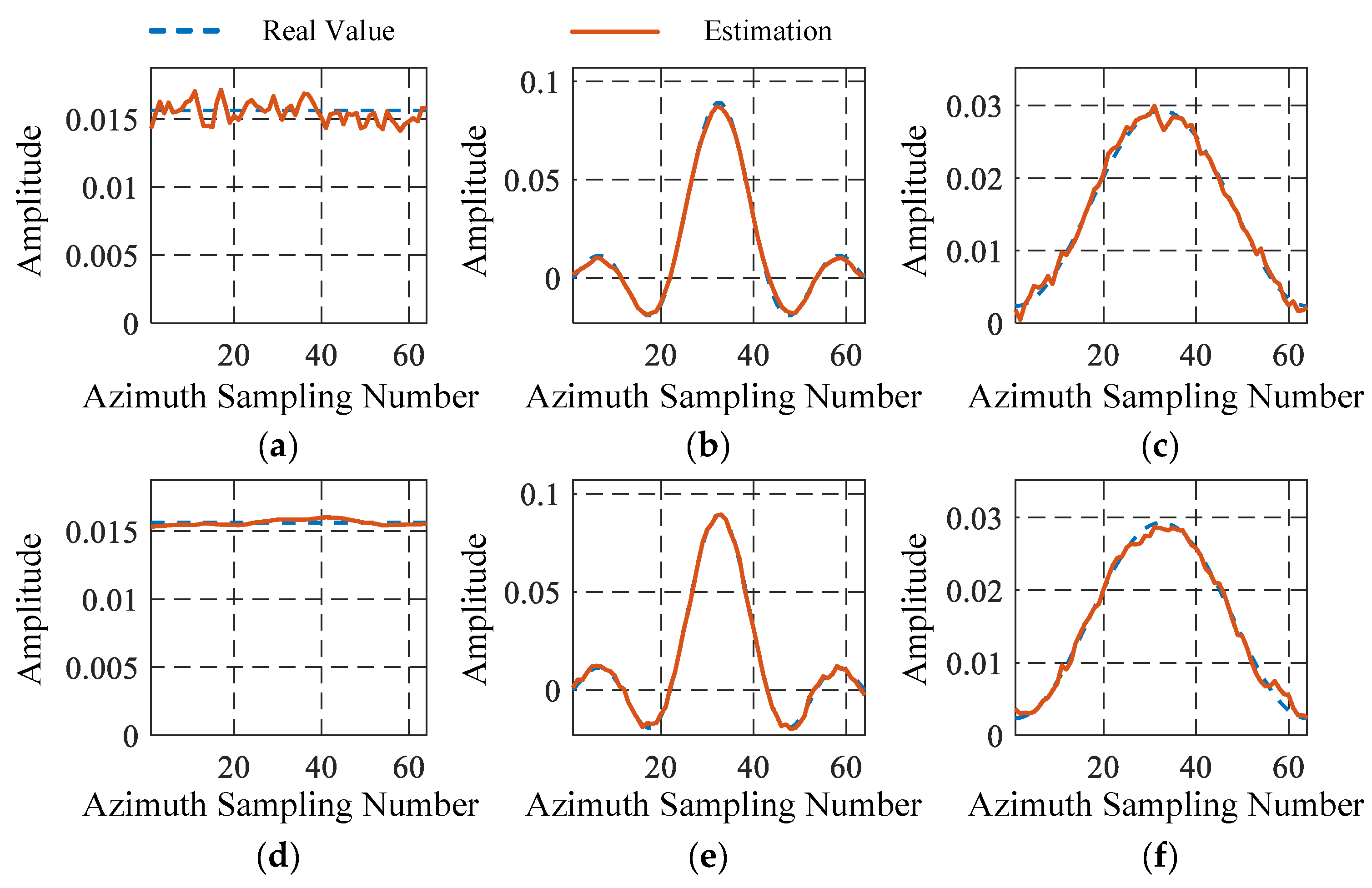
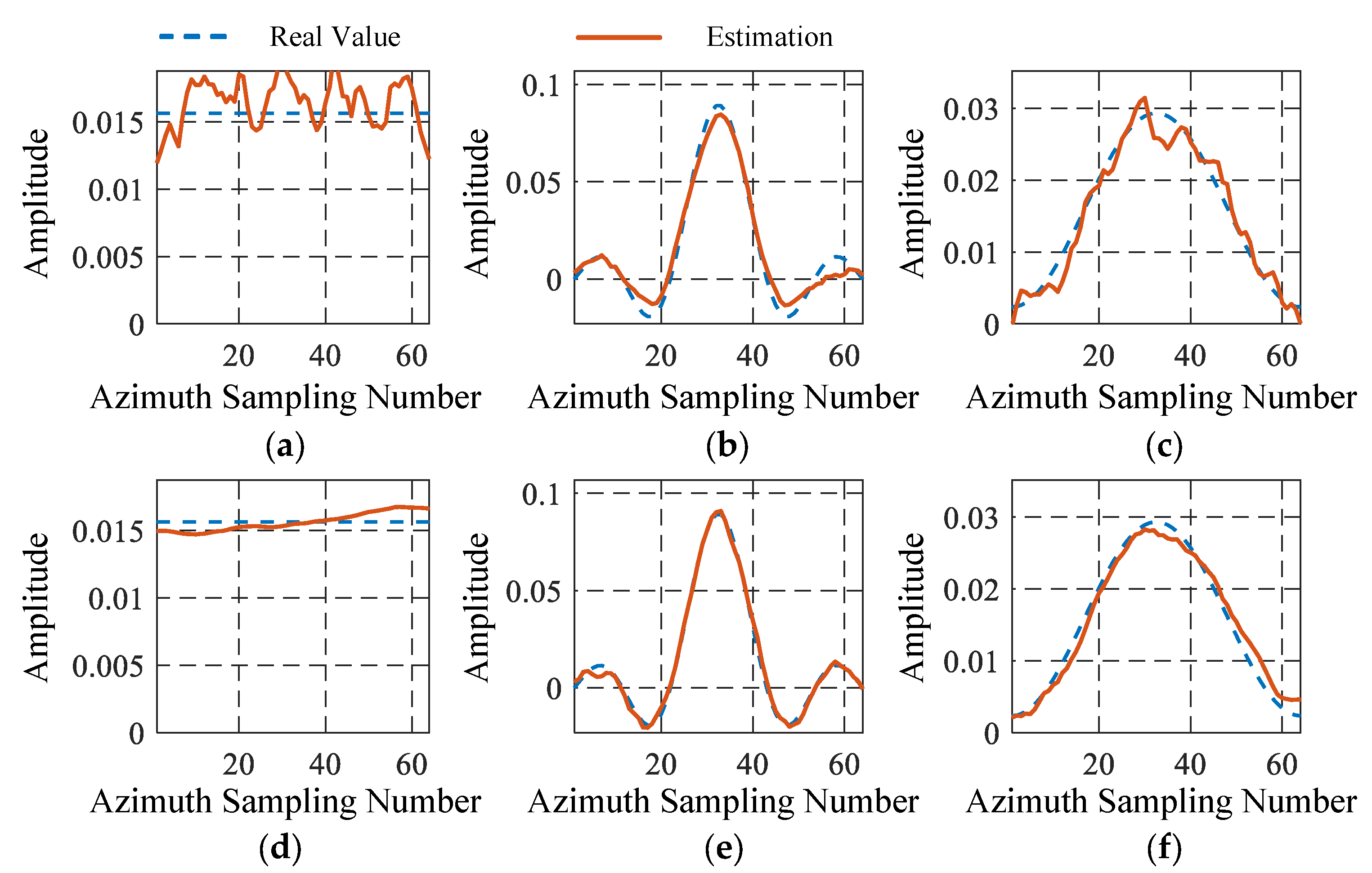
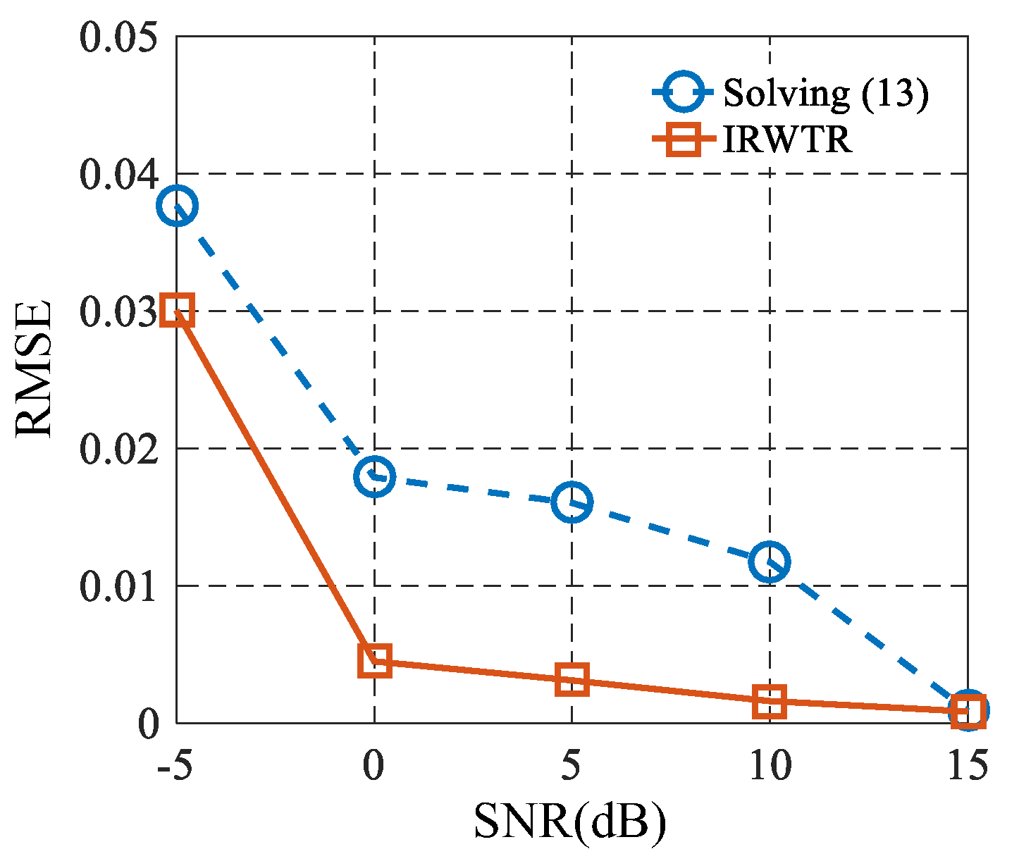
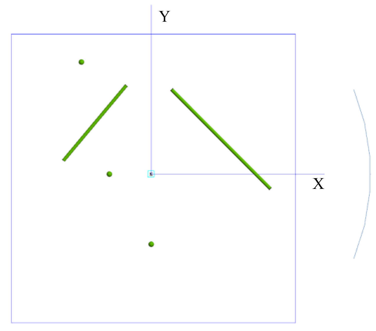
4.1. Results of Matlab Simulated Data and Analysis

The processing result of Matlab simulated data will be shown in this section. There are three scattering centers whose positions are ( 0 m , 1 m ) ( 0 m , 0 m ) and ( 1.5 m , 0 m ) , respectively, in the imaging scene. Their amplitude functions of azimuth were a constant, Sinc function and hamming window function. The radar transmitted step sweep frequency signal with a start frequency of 9.5 GHz and bandwidth of 1 GHz. The number of frequency signals was 32. The look angles ranged from −22.5° to 22.5°. The number of the look angles was 64.
Two methods were used to process the simulated data: solving (13) and the IRWTR algorithm. The processing was undertaken under different noise conditions (10 dB and 0 dB) and the results are shown in Figure 7 and Figure 8, where the blue dashed line shows the real value and the red solid line shows the estimation.
In Figure 7, the performance of the estimation of the Sinc-like amplitude function was the best. In contrast, the other estimations were inaccurate, for the regularization parameter was not large enough. This phenomenon is more significant in Figure 8. According to estimation of the Sinc-like amplitude function in Figure 8b, the regularization parameter was larger than the requirement, for the estimation was too smooth and deviated from the real values. In contrast, the regularization parameters for the rest amplitude functions were smaller than the requirement, which made the estimations oscillate. Compared with the regularization with a single regularization parameter, the MRP regularization provided better estimations. Both in Figure 7 and Figure 8, the estimations obtained via IRWTR were more close to the real values.
To evaluate the performance of different methods under different conditions of signal-to-noise ratio (SNR) SNR, a Monte Carlo simulation was used, in which 50 trials were performed for each SNR. In each trial, the relative mean squared error (RMSE) [17] was calculated. The statistical analysis is shown in Figure 9. In Figure 9, the performance of the IRWTR was more superior as SNR decreased.

4.2. The Results of Electromagnetic Simulation Data and Analysis

In this section, we apply the proposed processing procedure to the data simulated by FEKO software and the processing results will be shown.
The imaging scene is shown in Figure 10, which included two metal rods and three metal balls. The radar transmitted a step sweep frequency signal with a start frequency of 8 GHz, bandwidth 4 GHz. The azimuth start and end angle were −22.5° and 22.5°. We applied the BP imaging algorithm to the simulation data and the result is shown in Figure 11.
In Figure 11, there are only seven points. In fact, we knew that there were two distributed scattering centers in the scene from Figure 10. However, because their specific orientations, we could not recognize these two distributed scattering centers from Figure 11. We applied the proposed method in Section 3.2 to the data and extract the aspect-dependent amplitudes of all points. The estimated aspect-dependent amplitudes are presented in Figure 12. According to Figure 12, we can find that the amplitudes of certain scatterers were almost independent of the look angle. These scatterers with slowly varying amplitudes were the imaging results of the metal balls, which were the actual local scattering centers. The variations in the amplitude responses of the rest were more remarkable. The degrees of variation in amplitude responses could help us distinguish the ends of distributed scattering centers from the local scattering centers. Based on the azimuth-dependent scattering behaviors shown in Figure 12, the ends of distributed scattering centers are indicated by red circles in Figure 11.
The estimated aspect-dependent amplitudes of the scatterer 1, 2, 4, and 7 were compared with the ones calculated by FEKO. The comparisons are shown in Figure 13.
From Figure 13, it can be found that the estimated amplitudes corresponded closely with the ones calculated by FEKO. Moreover, we arranged the ends in pairs based on the extracted amplitudes. The signals to form the images of the flanks were constructed based on the arrangement and added to the original return signals. The imaging result of the reproduced data is shown in Figure 14. In Figure 14, the distributed scattering centers were easier to be distinguished from the local scattering centers.

4.3. The Results of the Backhoe Data and Discussion

In this subsection, we apply the proposed method to the backhoe data. The backhoe model is shown in Figure 15.
The corresponding processing results by the proposed method are presented in Figure 16b,e. The original imaging result of the backhoe with the look angles ranging from 25°to 70° is presented in Figure 16a. The portion within the white box in Figure 16a is shown in Figure 16d. The imaging result with the look angles ranging from −10°to 35° is shown in Figure 16c and the corresponding enlargement is shown in Figure 16f. In Figure 16a,d, some distributed scattering centers cannot be seen, which can be found in Figure 16c,f. The proposed algorithm was applied to the data with look angles ranging from 25° to 70° to restore the incomplete images of distributed scattering centers. The restored image is shown in Figure 16b,e. According to Figure 16b,e, some incomplete images of distributed scattering centers were restored.
However, in the restored image, we also found that some images of the distributed scattering centers were not restored correctly. According to the inaccurate restorations, we discussed some problems and limitations of the proposed method. In the discussion part, we mainly focus on the processing result of the bucket of the backhoe, whose images are within the white boxes in Figure 16.
The black and red lines in Figure 15 mark the distributed scatterers whose images are not complete in Figure 16d. The red lines in Figure 15 denote the distributed scatterers with the correctly restored images in Figure 16e, corresponding to the areas within the red dashed boxes. The distributed scatterers that were not restored correctly were marked by the black lines on the backhoe model in Figure 15. These scatterers correspond to the areas within the black dashed boxes. The two distributed scatterers marked by the black lines on the model were inside the bucket under the condition that the look angles ranged from 25° to 70°, since we can only find the images of their ends on one side in Figure 16e. Consequently, although the algorithm detected the two ends, it cannot perform the correct pairing, since the ends that can be correctly paired with them cannot be illuminated by the signals. However, the proposed algorithm has to find the ends to be paired with them. As a result, the wrong pairing occured. Another phenomenon we did not consider in this algorithm is the interactions [10] among the scatterers. Interactions among the scatterers are very common in a complex scene, especially for the bucket of the backhoe which can be regarded as a cavity. The interactions may give rise to the images of scatterers with wrong positions. This may influence the anisotropic characteristics extraction and the pairing.

5. Conclusions

A novel method for extracting anisotropic characteristics of scattering centers and the feature enhancement in the wide-angle SAR imagery was proposed in this paper. The main target of this study was to restore the incomplete images of the distributed scattering centers in a wide-angle SAR image based on the anisotropic characteristics. In the proposed scheme, firstly, the anisotropic characteristics were extracted by the proposed IRWTR algorithm. Secondly, the anisotropic characteristics were used to determine if a point in the SAR image was actually the image of an end of a distributed scattering center. Thirdly, these point-like images of the ends of distributed scattering centers will be lined up in pairs based on their anisotropic characteristics extracted by IRWTR.

Author Contributions

Y.G. conceived the main idea; M.X., L.G., and Z.Z. conceived and designed the experiments; Y.G. and M.X. analyzed the data and wrote the paper.

Funding

This research was funded by the Foundation for Innovative Research Groups of the National Natural Science Foundation, grant number 61621005 and the National Natural Science Foundation of China, grant number 61571349.

Acknowledgments

The authors would like to thank Jixiang Fu for his support in the data simulation.

Conflicts of Interest

The authors declare no conflict of interest.

References

  1. Ash, J.N.; Ertin, E.; Potter, L.C.; Zelnio, E.G. Wide-angle synthetic aperture radar imaging: Models and algorithms for anisotropic scattering. IEEE Signal Process. Mag. 2014, 31, 16–26. [Google Scholar] [CrossRef]
  2. Varshney, K.R.; Çetin, M.; Fisher, J.W.; Willsky, A.S. Sparse representation in structured dictionaries with application to synthetic aperture radar. IEEE Trans. Signal Process. 2008, 56, 3548–3561. [Google Scholar] [CrossRef]
  3. Xu, F.; Li, Y.; Jin, Y. Polarimetric-anisotropic decomposition and anisotropic entropies of high-resolution SAR images. IEEE Trans. Geosci. Remote Sens. 2016, 54, 5467–5482. [Google Scholar] [CrossRef]
  4. Duan, J.; Zhang, L.; Xing, M.; Wu, Y.; Wu, M. Polarimetric target decomposition based on attributed scattering center model for synthetic aperture radar targets. IEEE Geosci. Remote Sens. Lett. 2014, 11, 2095–2099. [Google Scholar] [CrossRef]
  5. Fuller, D.F.; Saville, M.A. A high-frequency multipeak model for wide-angle SAR imagery. IEEE Trans. Geosci. Remote Sens. 2013, 51, 4279–4291. [Google Scholar] [CrossRef]
  6. Liu, H.; Jiu, B.; Fei, Li.; Wang, Y. Attributed scattering center extraction algorithm based on sparse representation with dictionary refinement. IEEE Trans. Antennas Propag. 2017, 65, 2604–2614. [Google Scholar] [CrossRef]
  7. Ertin, E.; Moses, R.L. Through-the-wall SAR attributed scattering center feature estimation. IEEE Trans. Geosci. Remote Sens. 2009, 47, 1338–1348. [Google Scholar] [CrossRef]
  8. Potter, L.C.; Moses, R.L. Attributed scattering centers for SAR ATR. IEEE Trans. Image Process. 1997, 6, 79–91. [Google Scholar] [CrossRef] [PubMed] [Green Version]
  9. Gerry, M.J.; Potter, L.C.; Gupta, I.J.; Merwe, A.V.D. A parametric model for synthetic aperture radar measurements. IEEE Trans. Antennas Propag. 1999, 47, 1179–1188. [Google Scholar] [CrossRef]
  10. He, Y.; He, S.; Zhang, Y.; Wen, G.; Yu, D.; Zhu, G. A forward approach to establish parametric scattering center models for known complex radar targets applied to SAR ATR. IEEE Trans. Antennas Propag. 2014, 62, 6192–6205. [Google Scholar] [CrossRef]
  11. Altair FEKO™: A Comprehensive Computational Electromagnetics Code. Introduction. Available online: https://altairhyperworks.com/product/FEKO (accessed on 3 December 2018).
  12. Ulander, L.M.H.; Hellsten, H.; Stenstrom, G. Synthetic-aperture radar processing using fast factorized back-projection. IEEE Trans. Aerosp. Electron. Syst. 2003, 39, 760–776. [Google Scholar] [CrossRef]
  13. Xu, G.; Xing, M.; Zhang, L.; Liu, Y.; Li, Y. Bayesian inverse synthetic aperture radar imaging. IEEE Geosci. Remote Sens. Lett. 2011, 8, 1150–1154. [Google Scholar] [CrossRef]
  14. Ziniel, J.; Schniter, P. Dynamic compressive sensing of time-varying signals via approximate message passing. IEEE Trans. Signal Process. 2013, 61, 5270–5284. [Google Scholar] [CrossRef]
  15. Ziniel, J.; Schniter, P. Efficient high-dimensional inference in the multiple measurement vector problem. IEEE Trans. Signal Process. 2013, 61, 340–354. [Google Scholar] [CrossRef]
  16. Charles, A.S.; Balavoine, A.; Rozell, J.C. Dynamic filtering of time-varying sparse signals via L1 minimization. IEEE Trans. Signal Process. 2016, 64, 5644–5656. [Google Scholar] [CrossRef]
  17. Stojanovic, I.; Cetin, M.; Karl, W.C. Joint space aspect reconstruction of wide-angle SAR exploiting sparsity. In Proceedings of the SPIE—The International Society for Optical Engineering, Orlando, FL, USA, 15 April 2008; Volume 6970, pp. 1–12. [Google Scholar] [CrossRef]
Figure 1. Geometric model of the wide-angle SAR synthetic aperture radar (SAR) imaging.
Remotesensing 10 02066 g001
Figure 2. The imaging result of a metal rod under the condition that the incident direction is vertical to the flank occasionally during the acquisition. (a) Imaging scene. (b) SAR imaging result.
Remotesensing 10 02066 g002
Figure 3. The imaging result of a metal rod under the condition that the incident direction is not vertical to the flank during the acquisition. (a) Imaging scene. (b) SAR imaging result.
Remotesensing 10 02066 g003
Figure 4. Diagram of the proposed method. (a) The scene for imaging. (b) SAR imaging result. (c) Estimated anisotropic characteristics. (d) Enhanced SAR imaging result.
Remotesensing 10 02066 g004
Figure 5. The influence of σ p 2 .
Remotesensing 10 02066 g005
Figure 6. Flowchart of the proposed method.
Remotesensing 10 02066 g006
Figure 7. The comparison of the estimations from different methods (signal-to-noise ratio (SNR) = 10 dB). (a) Solution of (13) for the constant amplitude function. (b) Solution of (13) for the Sinc-like amplitude function. (c) Solution of (13) for the hamming-window amplitude function. (d) Iterative re-weighted Tikhonov regularization (IRWTR) solution for the constant amplitude function. (e) IRWTR solution for the Sinc-like amplitude function. (f) IRWTR solution for the hamming-window amplitude function.
Remotesensing 10 02066 g007
Figure 8. The comparison of the estimations from different methods (SNR = 0 dB). (a) Solution of (13) for the constant amplitude function. (b) Solution of (13) for the Sinc-like amplitude function. (c) Solution of (13) for the hamming-window amplitude function. (d) IRWTR solution for the constant amplitude function. (e) IRWTR solution for the Sinc-like amplitude function. (f) IRWTR solution for the hamming-window amplitude function.
Remotesensing 10 02066 g008
Figure 9. Performance comparison of the methods under different levels of noise.
Remotesensing 10 02066 g009
Figure 10. The imaging scene.
Remotesensing 10 02066 g010
Figure 11. The original imaging result.
Remotesensing 10 02066 g011
Figure 12. The aspect-dependent amplitudes of the scattering centers.
Remotesensing 10 02066 g012
Figure 13. The comparisons between the estimated and calculated amplitudes. (a) Scatterer 1; (b) Scatterer 2; (c) Scatterer 3; (d) Scatterer 4.
Remotesensing 10 02066 g013
Figure 14. The imaging result with the enhanced features.
Remotesensing 10 02066 g014
Figure 15. The model of the backhoe.
Remotesensing 10 02066 g015
Figure 16. Imaging results of the backhoe data. (a) Image corresponding to the look angles ranging from 25° to 70°. (b) The restored result of (a). (c) Image corresponding to the look angles ranging from −10° to 35°. (d) Portion of (a). (e) Portion of (b). (f) Portion of (c).
Remotesensing 10 02066 g016

