Numerical Mapping and Modeling Permafrost Thermal Dynamics across the Qinghai-Tibet Engineering Corridor, China Integrated with Remote Sensing

Abstract

Permafrost thermal conditions across the Qinghai–Tibet Engineering Corridor (QTEC) is of growing interest due to infrastructure development. Most modeling of the permafrost thermal regime has been conducted at coarser spatial resolution, which is not suitable for engineering construction in a warming climate. Here we model the spatial permafrost thermal dynamics across the QTEC from the 2010 to the 2060 using the ground thermal model. Soil properties are defined based on field measurements and ecosystem types. The climate forcing datasets are synthesized from MODIS-LST products and the reanalysis product of near-surface air temperature. The climate projections are based on long-term observations of air temperature across the QTEC. The comparison of model results to field measurements demonstrates a satisfactory agreement for the purpose of permafrost thermal modeling. The results indicate a discontinuous permafrost distribution in the QTEC. Mean annual ground temperatures (MAGT) are lowest (<−2.0 °C) for the high mountains. In most upland plains, MAGTs range from −2.0 °C to 0 °C. For high mountains, the average active-layer thickness (ALT) is less than 2.0 m, while the river valley features ALT of more than 4.0 m. For upland plains, the modeled ALTs generally range from 3.0 m to 4.0 m. The simulated results for the future 50 years suggest that 12.0%~20.2% of the permafrost region will be involved in degradation, with an MAGT increase of 0.4 °C~2.3 °C, and the ALT increasing by 0.4 m~7.3 m. The results of this study are useful for the infrastructure development, although there are still several improvements in detailed forcing datasets and a locally realistic model.

1. Introduction

Permafrost is a significant and sensitive phenomenon of the terrestrial cryosphere. Since the last little ice age, most near-surface permafrost has been degrading and the rate has increased recently, as evidenced by permafrost temperature increasing and the positive trend of the active-layer thickness, as consequences of climate change [1]. Permafrost degradation is likely to have wide influences on surface and subsurface hydrologic conditions, soil strength properties, and ecosystems [2]. The Qinghai-Tibet Plateau (QTP) has the largest lower latitude permafrost region (1.06 × 10⁶ km²) in the world [3,4]. During the last decades, permafrost warming has been widely reported on the QTP [5,6,7,8]. Changes in the active-layer thickness and permafrost temperature due to climate warming and surface disturbances have major ecological and engineering implications [9,10,11,12], such as stability of slopes and thermokarst [13,14,15]. Ongoing climatic change and its associated effects on ground thermal dynamics, and natural hazards make it important to map the permafrost thermal state on the QTP. A new expressway from Golmud to Lhasa has been proposed along the Qinghai–Tibet Engineering Corridor (QTEC) across the QTP. Since the engineering design and cost of road construction will be affected by the permafrost condition, a detailed and present knowledge of permafrost thermal state is essential. Present available permafrost maps are mainly at low resolutions, although many permafrost maps have been compiled since the early 1960s [4,16,17,18]. These coarse resolution studies are not suitable for land-use planning. Niu et al. [19] gave a coherent picture of permafrost distribution in the QTEC, but did not reproduce active-layer thickness and permafrost temperature. These studies above do not access the future permafrost degradation due to climate change. Therefore, improved methods for mapping permafrost thermal dynamics are essential for designing road and pipelines, and ecological assessment in the QTEC.

Mapping of permafrost distribution, especially its thermal state, remains a challenging problem due to the scarcity of observed data. Many models already exist for estimating the spatial distribution of permafrost in regions of the European Alps [20,21,22], and Arctic environment [23,24]. These models may be of the equilibrium, empirical–statistical, or process-based types, and have been widely used at regional and local scales [25,26,27,28]. The applicability of equilibrium models is restricted to relatively simple problems, and where the transient effects may be unimportant. Transient numerical modeling with incorporated phase change effect is the most effective method to simulate and forecast the thermal regime of permafrost over a relatively short time interval, where the transient effects of phase change are important.

Therefore, the target of this study is to model and map the permafrost thermal regimes in the QTEC (91°E~95°E, 32°N~36°N) based on a numerical Geophysical Institute Permafrost Laboratory (GIPL 2.0) model, which solves the 1-D heat transfer equation accounting for phase change of soil water. This model has been successfully applied for the first time to the entire QTP permafrost domain with 0.1° spatial resolution by Qin et al. [18]. We investigate the surface characteristics (e.g., vegetation, soil) and permafrost conditions along the QTEC based on the permafrost survey positions and boreholes that were carried out when the Qinghai–Tibet railway (QTR) and Qinghai–Tibet highway (QTH) were built. The remote sensing helps to upscale the forcing data and ground properties to the entire corridor. Consequently, we simulate the permafrost thermal state and its dynamics in the future with 1 km by 1 km spatial resolution to cover the QTEC region. This resolution is based on the use of the remote sensing datasets.

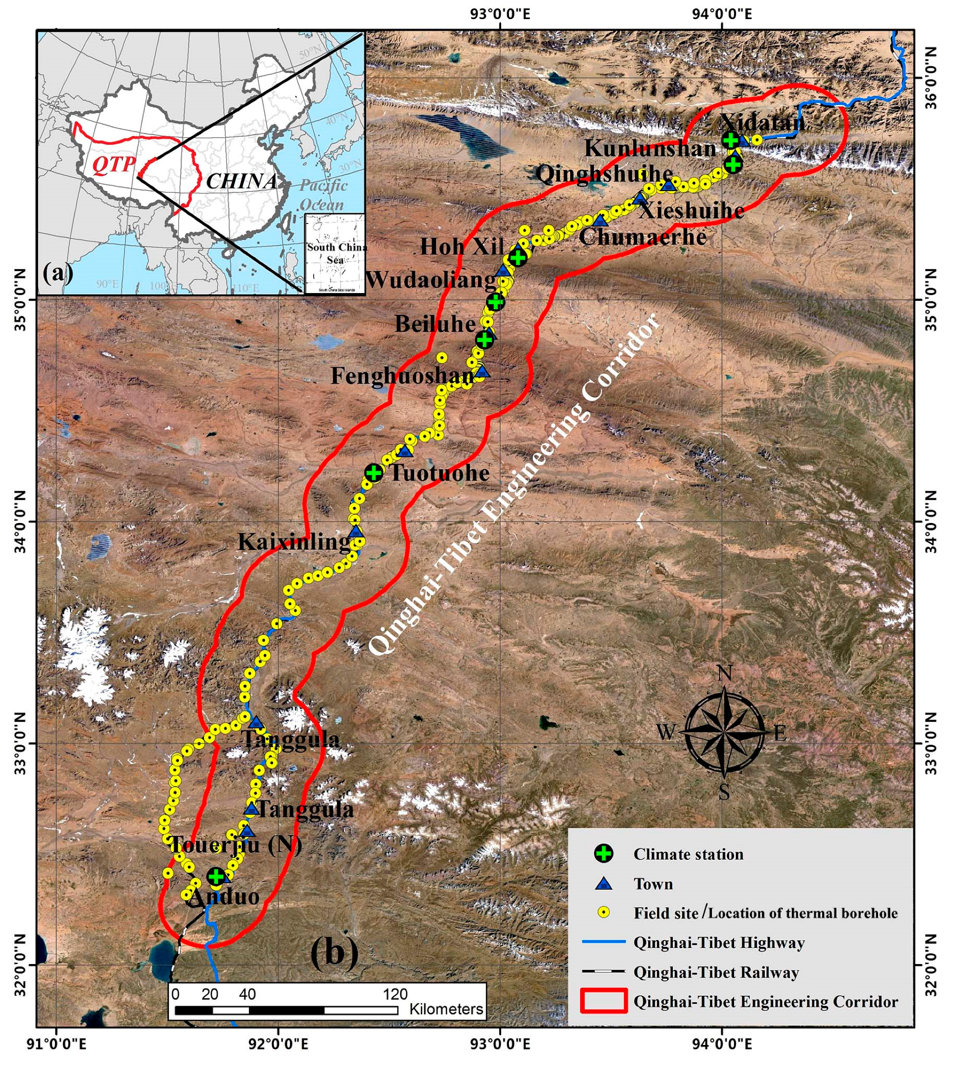
2. Study Area

The study area is located in the central QTP and encompassed a 550 km long and 40 km wide section of the QTP, covering an area of around 22,351 km². This area extends from Xidatan to Anduo (northern and southern boundary of permafrost occurrence, respectively), bounded by latitude 32~36°N and longitude 91~95°E [29] (Figure 1). This corridor is likely to become a locus of many developmental projects because construction of a gas pipeline, QTH, QTR, and electric transmission lines are along this route. Most parts of the terrain are located 4500 m a.s.l., with an alternating distribution of mountains (e.g., Kunlunshan, Fenghuoshan, and Tanggula), valleys (e.g., Xieshuihe, Tuotuohe, and Qingshuihe), and upland plains (e.g., Chumaerhe, Wudaoliang, and Beiluhe). Recent field investigations and literatures indicate that near surface deposits are dominated by coarse materials such as gravel and sandy soils [6,10]. These specific geomorphologic and sedimentary patterns result in significant differentiations in permafrost features [10]. Climatically, it is located in an extremely continental climate zone, favoring clear skies and high solar radiation. The mean annual air temperatures (MAAT) are commonly between −6.5 °C and −2.0 °C, with the annual total precipitation ranging from 250 mm to 450 mm which occurs mostly as rainfall between May and August [6,8,30]. The majority of the plateau has a free snow cover in winter [30]. Vegetation type is characterized as alpine meadow, degraded alpine meadow, alpine steppe, and sparse grassland with the coverage ranging from 0.15 to 1.0 [19]. The QTEC is dominated by discontinuous permafrost (occupying 60.3% of the study area) with relatively “warm” ground temperatures (i.e., mean annual ground temperature at 15 m depth, MAGT), which are above −4.0 °C based on the available thermal borehole data [19]. In the present time, the active-layer thickness (ALT) ranges from 0.8 m to 7.5 m [8,19,30].

3. Methods

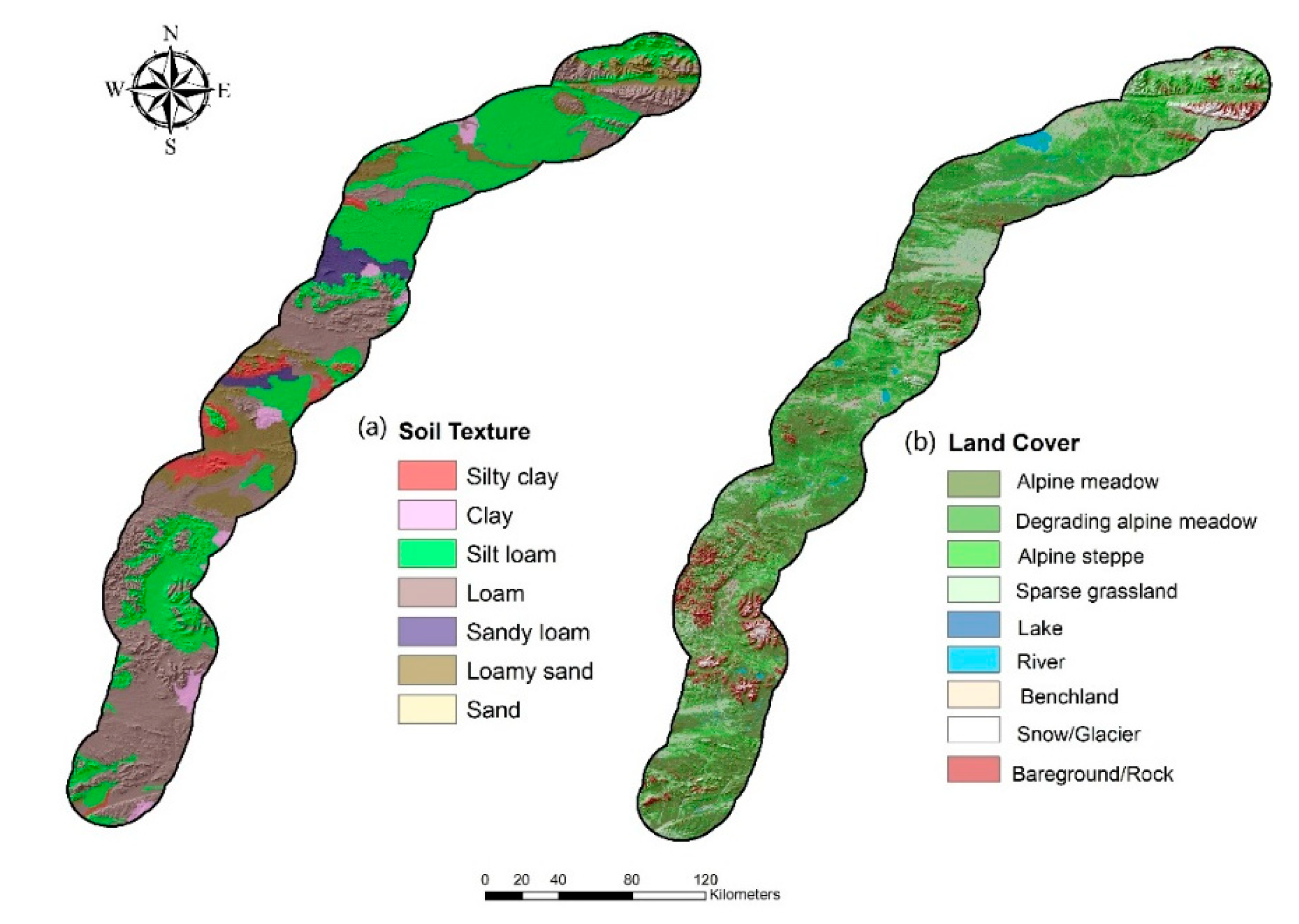
3.1. Field Data

Five major field data sources are used for this study (Figure 1b). One is 33 the thermal boreholes along the QTH and QTR, which was published by Wu and Zhang [6,7], and Wu et al. [30]. These boreholes were conducted in the 1970s, with a depth of 15.0 m. In each borehole, a calibrated thermistor cable (accuracy ± 0.05 °C) was installed to measure permafrost temperature 2 times in a month. In this study, we use ground temperature of the last 10 years to obtain general information about permafrost temperature change (2003–2012). The second is 300 geological and ground thermal survey boreholes by the Road Survey and Design Institution during the period from August 2015 to October 2015 (15 m depth) which covers most of the corridor and provides general information about geology, geomorphology, and soil hydrology [19]. Based on these borehole locations, we carried out investigations on soil thermal properties in different alpine ecosystems. The third is a detailed ecosystem classification of the corridor in Niu et al. [19]. This high resolution (2.0 m) classification was produced by using object-oriented classification and visual interpretation methods. The fourth is seven available Onset HOBO climate stations in this study which provide general information about the climate in the QTEC. They are located in different terrains (Figure 1b), and record the air temperature (2.0 m above the ground surface) every 4 hours for a long period (1957–2016). In this study, the daily mean air temperature is calculated to provide the long-term near-surface air temperature changing trend. In a companion study [19], we have shown the field data details and the method of ecosystem classification. Based on these field sites, we carried out vegetation and soil surveys in August–October 2016. Soil thermal properties were measured using a portable thermal characteristic analyzer (KD 2 Pro, Decagon, USA) with an accuracy of 95% for the volumetric heat capacity (C), 95% for the thermal conductivity (k), and 90% for the thermal diffusivity (D). These data are complemented with other data from satellite images and databases, such as will be explained in Section 3.2.2.

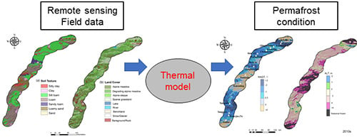
3.2. Permafrost model GIPL2.0

For this study, we make use of GIPL 2.0 numerical transient model which is capable of representing the freezing and thawing cycle. This model is developed by Tipenko et al. [31], and has been successfully applied to entire Alaskan [23] and the QTP permafrost region [18]. This model solves the 1-D heat transfer equation accounting for phase change of soil water (Equation (1)). Heat conduction is assumed as the only process of energy transfer in the model.

$$\frac{\partial H\left(x,T\right)}{\partial t}-\nabla \cdot \left(k\left(x,T\right)\frac{\partial T\left(x,t\right)}{\partial x}\right)=0,$$

(1)

where T (x, t) is the soil temperature, x and t are the soil depth and time respectively, k (x, T) is the soil thermal conductivity (W/(mk)), and H (x, T) is the enthalpy (Equation (2)).

$$H\left(x,T\right)={\int }_0^{T}C\left(x,s\right)ds+L\Theta \left(x,T\right),$$

(2)

where C (x, s) is the volumetric soil heat capacity (MJ/(m³ K)), Θ (x, T) is the soil volumetric unfrozen water fraction, and L is the volumetric latent heat of fusion (MJ/m³).

The volumetric content of liquid water with temperature is the freeze curve of soil and depends on soil composition and structure. The model does not account for changing subsurface water contents, but instead assigns fixed values for the porosity and saturation of each grid cell. The formula for Θ (x, T) is defined as follows (Equation (3)):

$$\Theta \left(x,T\right)=\eta \left(x\right)\{\begin{array}{l}1,T\ge T_{\ast }\\ a{\left|T\right|}^{-b},T<T_{\ast }\end{array}.$$

(3)

where a and b are coefficients of unfrozen water curve, η(x) is the volumetric moisture content. T_※ is a freezing point depression. Detailed description of this model can be found in Jafarov et al. [23].

3.2.1. Model Setting, Boundary, and Initialization

At 1 km resolution, the soil and ground profile domain is generated with 139 vertical grid cells to a depth of 100 m. The size of the cells increases with depths with a minimum grid cell spacing of 0.1 cm for the shallow soils and maximum spacing of 10 m at the bottom. Soil profile includes fibrous horizons, mineral soils, and bedrock. The upper boundary conditions are determined on the ground surface temperature which can reflect the effects of land surface (e.g., vegetation and snow), and the lower boundary conditions are defined based on the geothermal gradient of 0.07 °C/m, as estimated from a deep borehole [30]. The model initialization conditions are defined by a temperature distribution in the ground material. In this study, we extrapolate the available initial ground temperature profiles to the whole QTEC using regression analysis [18]. The details of initialization are shown in Section 3.2.2.

3.2.2. Model Forcing Datasets

GIPL 2.0 requires a synthesized time series of land surface temperature as forcing data sets. The forcing data covers a period from 1980 to 2015 which is divided into a target period ranging from 2010 to 2015 and a spin-up period from 1980 to 2009. Generally, a pronounced increase in air temperature and precipitation started after the 1980s (Figure 2). It is reasonable to presume the climate was steady before the 1980s. Therefore, the permafrost around the 1980s is assumed in equilibrium. To estimate a realistic initial temperature profile, the model is spun up using a repeated 30-year period from 1980 to 2009 with a constant average soil temperature (Ti) obtained in Section 3.2.1. During the spin-up period (1980–2009), the required surface temperature forcing is extracted from the China Meteorological Forcing Dataset (http://dam.itpcas.ac.cn/rs/?q=data#CMFD_0.1). This product provides eight time daily gridded near-surface air temperatures since 1981 with a spatial resolution of 0.1°. It is extensively validated and found to be in good agreement with meteorological observations on the QTP [32,33]. The coarse scale surface temperature values of the reanalysis product are interpolated to the location of the study site using a lapse-rate model [19]. During the target period (2011–2015) the surface temperature forcing is based on the remote sensing data, i.e., MODIS-LST products (MOD11A1/A2, MYD11A1/A2) with a spatial resolution of 1 km, which are a useful tool for permafrost modeling [34,35]. The passive remote sensing signal is strongly affected by water bodies, which show very different brightness temperatures [36,37]. Therefore, water bodies are masked out using the landscape classification which is compiled by Niu et al. [19]. The lakes and other open water bodies are excluded from our further analysis. Compared with field observations in 6 field sites (

Table 1. Correlation coefficient (R²), root mean square error (RMSE), and mean bias error (MBE) between MODIS-LST and field observations for different vegetation covered terrains.

Site Name	Surface Type	R2	RMSE	MBE
Xidatan	Alpine steppe	0.88	2.98	−0.02
Kunlunshan	Alpine meadow	0.92	2.64	0.46
Wudaoliang	Alpine meadow	0.87	3.13	−0.67
Beiluhe	Alpine steppe	0.91	2.32	0.29
Tuotuohe	Alpine steppe	0.85	3.54	−1.27
Anduo	Alpine meadow	0.81	4.5	−1.34

), the MODIS-LST is close to the observed surface temperature with a strong positive correlation (R² > 0.8). The mean bias errors (MBE) range from −1.34 °C to 0.46 °C with root mean square errors (RMSE) between 2.32 °C and 4.50 °C. This dataset has been generated by Niu et al. [19]. In order to evaluate the potential permafrost dynamics in the future 50 years under a warming climate, a constant warming trend is supposed in this study. A sine function with a constant warming rate for future near-surface air temperature change is assumed. We consider three warming scenarios with warming rates of 0.02 °C/year, 0.05 °C/year, and 0.07 °C/year, respectively. These rates are simulated based on the field observations of near surface air temperature over the last 30 years by using the linear fitting approach, as shown by the shadow in Figure 2. They represent the low, medium, and high rate of temperature increase from different climate stations across the QTEC. In addition, the ground surface temperature warming rate is assumed to be uniform with climate pattern.

3.2.3. Subsurface Properties and Model Parameters

According to the geological information from boreholes, three vertical soil layers are defined in the study area. Based on China Soil Map Based Harmonized World Soil Database (v1.1) at 1 km resolution, we distinguish seven soil texture categories for the top soil layer (0~100 cm) as the predominant subsurface stratigraphies within the QTEC. Figure 3a illustrates their spatial distribution. Most of the QTEC is covered by silty loam and loamy sand with some silty clay and sandy loam in the central QTEC. We delineate three typical geomorphological units as high mountain, river valley, and upland plain, which have distinctly different characteristics regarding their surface and subsurface properties, such as ground ice contents, thermokarst features, and vegetation cover. We define subsurface stratigraphies (intermediate layer) as clay based on the geomorphological units and available field investigations of soil properties according to the boreholes (Section 3.1). The bottom mineral layer is defined as rock for the entire study area. Spatially, there are about 32,000 1 km × 1 km pixels in the QTEC, indicating that it is not practical to simulate each pixel due to the computation time required and the model code framework. Similarly to Zhang et al. [38] and Nicolsky et al. [39], we employ the ecosystem types interpreted by Niu et al. [19] to parameterize the thermal properties of the soil texture, excluding rivers and lakes. This 2.0 m resolution land cover map delineates local-scale ecosystems that divide geomorphic, hydrologic, and pedologic characteristics of the ground (Figure 3b). Each ecosystem type is associated with closely related soil types. Therefore, we combine the ecosystem type and soil texture into ecosystem–soil pairs, such as alpine meadow-sand, alpine meadow-clay. After combinations of the ecosystem types and mineral soil types, we define uniform ground thermal properties for each pair based on field measurements using a portable thermal characteristic analyzer (KD 2 Pro, Decagon, USA, see Section 3.1). For each 1 × 1 km grid cell, the dominate ecosystem–soil pair class is determined. Finally, we obtained 88 unique pairs for the study area.

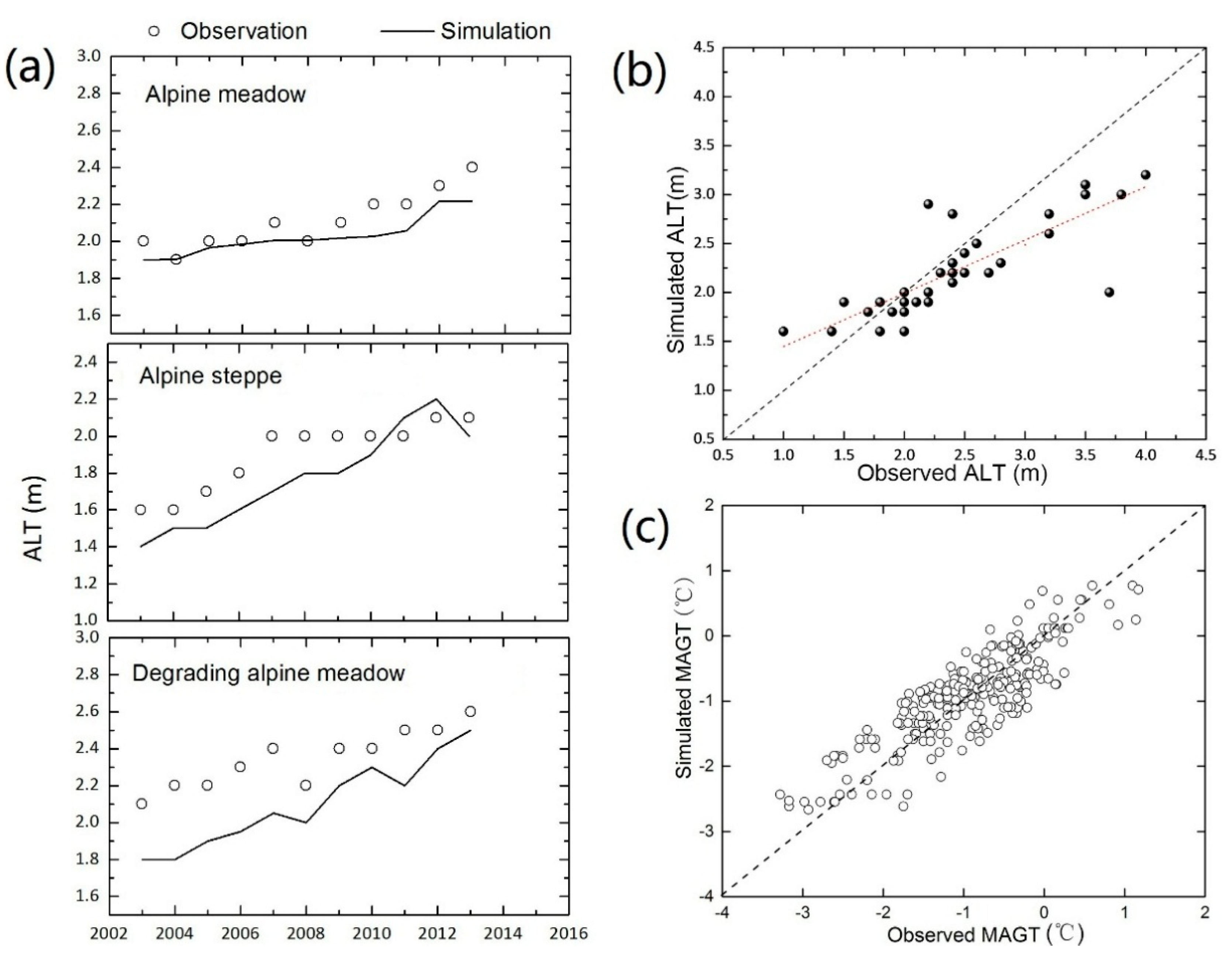
3.2.4. Model Validation

In this study, we compare the modeled ALT and MAGT to field observations during the period 2003–2014 based on the field data availability (Figure 4). The comparison of the interannual variability of the simulated and observed ALTs is exhibited in Figure 4a. Although there is some bias error (mean bias error < 0.25 m) in different geomorphological units and ecosystems, the simulated ALT follows the observed ALT dynamics. In addition, the scatterplot of simulated and observed ALT (33 sites) shows a good correlation (correlation coefficient, R² = 0.75) (Figure 4b). In terms of the MAGT, the simulated MAGT closely follows the observed pattern with a R² value of 0.85 as shown in Figure 4c. The above results have a strong agreement with the study in Qin et al. [18] that evaluated the performance of the GIPL 2.0 model using available observations. Therefore, the simulated ALT and MAGT are in good agreement with the in-situ measurements, although there is some bias error, indicating the validity of GIPL 2.0 model for obtaining the ALT and permafrost thermal state in the QTEC.

4. Results

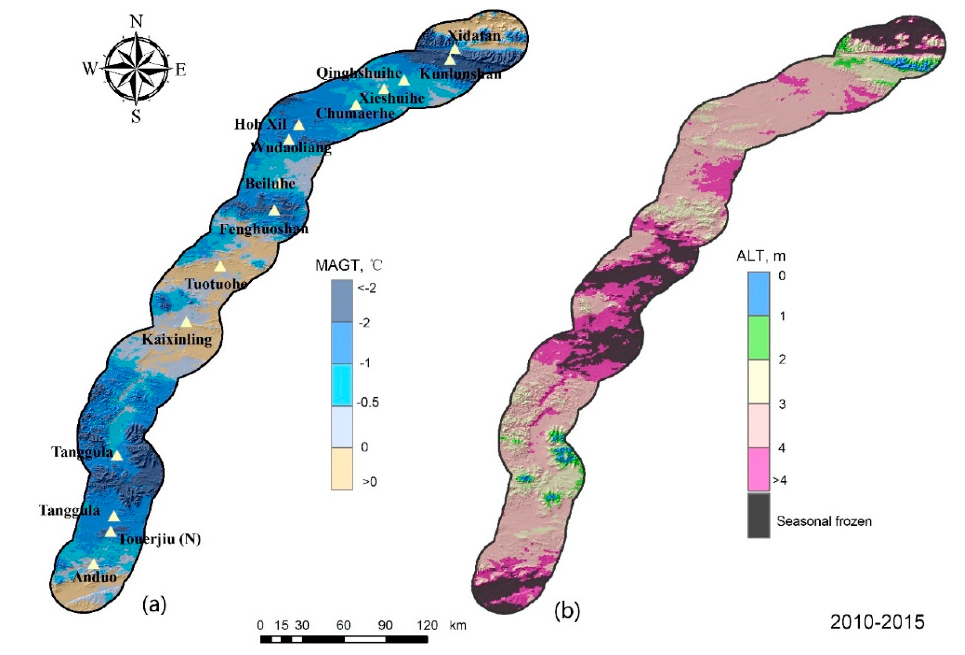
4.1. Spatial Distribution

Figure 5 presents the modeled average ground temperatures at 15 m depth (i.e., MAGT) and maximum thaw depths (ALT) for the period 2011–2015 at a grid resolution of 1 km. As shown in Figure 5a, the ground stratigraphic units generally have a pronounced impact on the MAGT. The modeled MAGTs are lowest for the high mountain areas, such as Kunlunshan, Tanggula Mountain with the temperature less than −2.0 °C, and highest for river valley areas, such as Tuotuohe with the temperature above 0 °C. As expected, the modeled MAGTs are above 0 °C in Xidatan and Anduo—north and south boundary of permafrost extent on the QTP. For upland plain areas (e.g., Beiluhe basin and Wudaoliang basin) the relatively warm MAGTs, ranging from −2.0 °C~0 °C, are mapped. Considering a MAGT <0 °C as the threshold for permafrost occurrence, the permafrost covers 78.9% of the study area, excluding rivers and lakes. Therefore, the permafrost extent in our study is discontinuous (underlying 50%~90% of the land surface).

The spatial distribution patterns of the modeled ALT are highly related to the MAGT (Figure 5b). Generally, permafrost areas with a colder MAGT (e.g., Kunlunshan, Tanggula) have relatively thinner ALTs, while the areas with warmer MAGTs are covered by thicker ALTs, such as in Tuotuohe. In high mountain areas, average ALTs of less than 2.0 m are modeled, while the river valley features ALTs of more than 4.0 m. For upland plain areas, the modeled ALTs generally range from 3.0 m to 4.0 m.

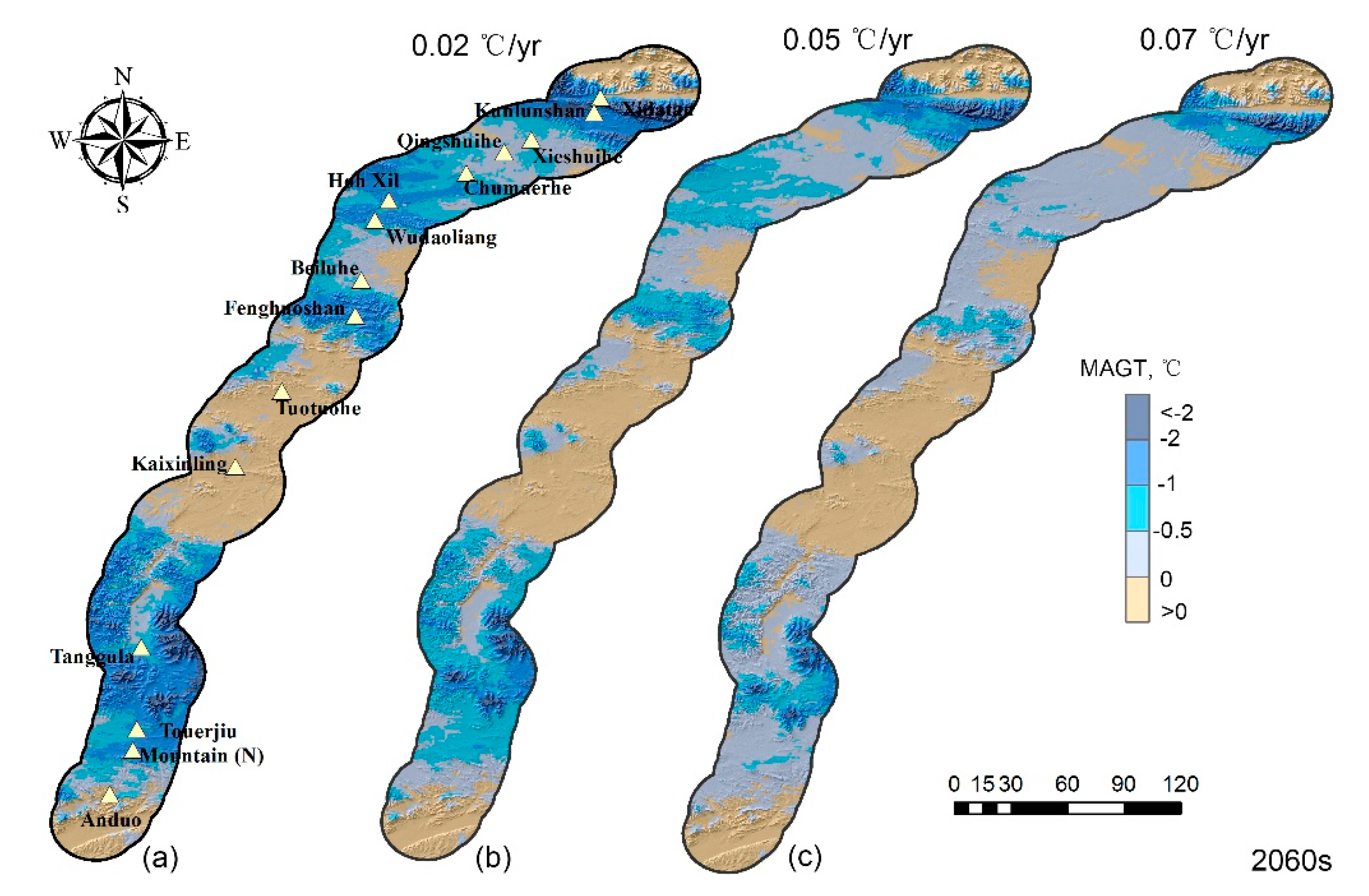
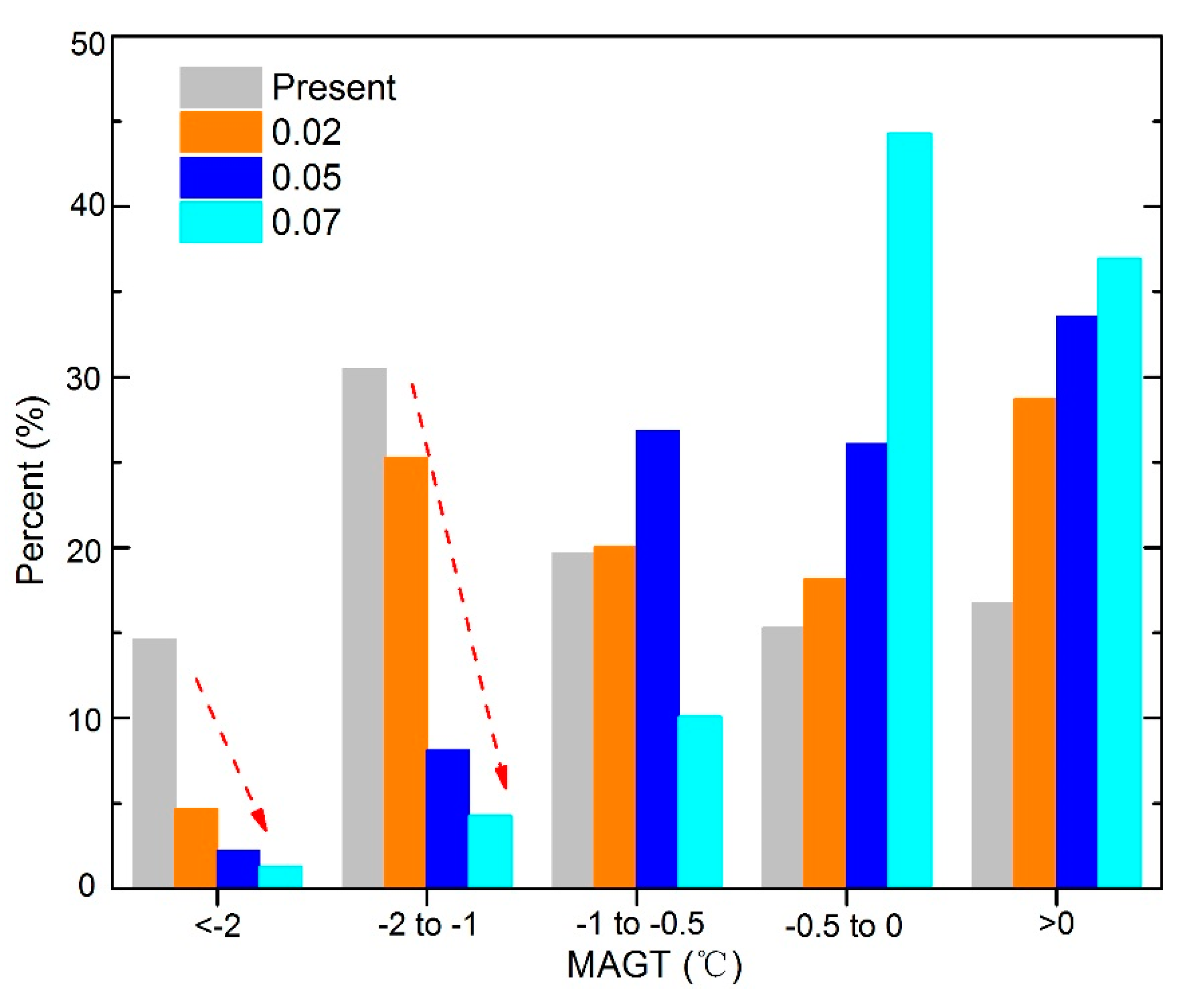
4.2. Future Permafrost Change in a Warming Climate

The spatial distribution of the MAGT for the period of the 2060s is depicted in Figure 6. In general, compared with present-day conditions, the overall area covered by MAGT less than 0 °C is going to decrease at different rates under the three climate warming scenarios. Results of the calculation show that about 2734.8 km² (12.0%), 3845.1 km² (16.8%), and 4616.5 km² (20.2%) will be involved in the widespread permafrost degradation under climate warming rates of 0.02 °C/year, 0.05 °C/year, and 0.07 °C/year, respectively. The average modeled MAGT will increase by 0.4 °C~2.3 °C at the end of the 2060s up to the climate change. Figure 7 indicates that changes in permafrost temperatures will be much pronounced within the areas with colder permafrost (MAGT < −1.0 °C, as red arrows shown) in comparison with areas where the permafrost temperature is presently close to 0 °C. The permafrost will be probably disappeared in drainage channel areas, such as Tuotuohe and Kaixinling. It will not increase significantly in the peaks of the high mountain, such as Tanggula and Kunlunshan. From the 2010s to the end of 2060s, modeled average ALT for the whole QTEC permafrost domain will probably increase by 0.4 m, 3.7 m, and 7.3 m under the scenarios of 0.02 °C/year, 0.05 °C/year, and 0.07 °C/year, respectively, indicating a significant response to scenario of climate change.

5. Discussion

5.1. Uncertainties Related to Model Forcing and Thermal Properties

This study maps permafrost thermal conditions and changes with climate (primary drivers of landscape-level permafrost extent) in the QTEC using a numerical model. Several uncertainties of this work are noteworthy. Firstly, this study uses the satellite remote sensing data (i.e., MODIS-LST) as the forcing dataset. Previous studies have revealed a cold bias of long-term averages from MODIS-LST in permafrost regions [19,35,40]. The same bias of 0~1.5 °C is found in most sites over our study area (Table 1), which may be attributed to (i) deficiencies of satellite observation during noontime when the temperature is warmest, and (ii) mixed pixels covering different vegetation types and water bodies within the 1 km² grid cells [36]. This cold-bias may introduce a slight cold bias in modeled ground temperature, which leads to the simulated ALT thinner than the measured one (Figure 4a,b). However, remote sensing data is an adequate choice to scale up the surface temperature distribution on the QTP because meteorological stations are scarce and widely scattered in those vast and remote regions. Another forcing uncertainty is the future climate projections which are based on the history observations. The hypothesis of a linear increase in air temperature is just a qualitative prediction of future climate change, which is a challenging work. In terms of future climate uncertainty, the results of model MAGT and ALT for the 2060s can qualitatively reveal the permafrost degradation with climate change and are to be used for trend analysis. Therefore, coupling with the global climate model (GCM) results should be considered in the future work [2].

Secondly, satellite data now can provide high spatial resolution maps for land cover and vegetation conditions, but soil maps are still very coarse across the QTEC. In this study, we estimated soil thermal parameters (i.e., kt/kf, Ct/Cf ) based on observations and ecosystem types. Recent studies on the sensibilities and uncertainties of the GIPL 2.0 model showed that the most influence on the simulated MAGT and ALT is the frozen thermal conductivity (kf) [18,39,41]. Soil type and thermal conditions, however, may differ widely within an ecosystem type. Therefore, improving the information about ground stratigraphy at a local scale is significant not only for permafrost modeling, but also for ecosystem assessment and infrastructure development under a warming climate. In addition, effects of potential changes in ecosystems on ground thermal regimes are not included in our model. It is necessary to incorporate a dynamic vegetation module into the permafrost model in future study.

And finally, GIPL 2.0 model is still one-dimensional, ignoring the lateral heat flux or subsidence due to ground ice melt which can modify the ground thermal regime [42,43]. However, at the one-kilometer distance, lateral heat flux may slightly affect soil thermal state because the number of sharp mountain slopes and open water areas in one grid cell is limited in our study. Climate change and human disturbances have significant impacts on vegetation conditions and permafrost thermal regimes through their effects on energy exchanges between the land surface and the atmosphere [44]. However, the application of a high-complexity model is still a challenge due to large computational resource requirement [45] and poor knowledge of the spatial model parameter sets [46].

5.2. Comparison with Other Observations and Results

Although latest studies have mapped permafrost on the QTP at different spatial resolution and considered topographic effects [4,18,19], they assumed that permafrost conditions are in equilibrium with climate or the resolution is coarse. Field observation for ground temperature and modelling studies have suggested that the current and future permafrost thermal conditions are not in equilibrium with the changing climate [2,47]. The latest high-resolution (30 m) permafrost probability map of the QTEC is compiled by Niu et al. [19], but does not represent active-layer thickness and ground temperature. A direct comparison of our result to the permafrost probability map shows that about 18.6% of the study area remains different (Figure 8). The differences mainly distribute over the drainage channels and flat terrains such as Tuotuohe river region with a relatively warm MAGT (−1.0 °C~0 °C). The empirical–statistical model described the distribution of permafrost based on geomorphological permafrost indicators, topographic, and climatic predictors [26]. Therefore, these empirical–statistical model results can poorly represent areas underlain by deep permafrost, which has a slight relation with ground surface conditions. This study therefore reveals more spatial details about the transient impact of climate change on permafrost in the QTEC.

Overall, compared to previous studies [4,8,18,19,30], the permafrost modelling approach used in this work integrates remote sensing products gives insights into the permafrost thermal regime and dynamics with climate change.

5.3. Changes in Active-Layer Thickness and Permafrost Distribution

The average increase in MAAT has been 1.0 °C~2.0 °C during the past 50 years across the QTEC (Figure 2). Ongoing climate warming and wetting have led to significant degradation of permafrost [1]. The model results show that the average ALT is likely to be increased by 3.7 m under the warming rate of 0.05 °C/year at the end of 2060s. This is much closer to 3.1 m~3.9 m over a period from 1995 to 2010, reported by Wu and Zhang [7] and Wu et al. [8]. According to the MAGT increasing rate of 0.02 °C/year over a period from 2006 through 2010 [8], the average MAGT will rise by 1.0 °C, which is consistent with the 0.4 °C~2.0 °C in this study. As shown in Figure 7, the degradation will firstly occur in areas that the MAGT is cold (MAGT < −1.0 °C) due to latent heat for melting. These warmings could lead to geotechnical problems and potential hazards in areas with relative cold MAGT in the QTEC. In this study, the permafrost thermal map can serve as an up-to-date resource to assess permafrost conditions and insights into mountain research.

6. Conclusions

In this study, a 1-D numerical permafrost model (GIPL 2.0) provides an insight into permafrost thermal dynamics in the Qinghai–Tibet Engineering Corridor at 1 km resolution, integrated with field, remote sensing and database data. Ecosystem types and near-surface soil types are derived from the satellite data and reanalysis products. Soil thermal conditions are scaled up based on ecosystem types and field observations. As forcing data, we obtained the daily average land surface temperatures from MODIS-LST products and reanalysis products. The future climate change scenarios are assumed based on historical station observations across the QTEC. From this study the following conclusions can be drawn:

(1) Integrated with field, remote sensing, and database data, the GIPL 2.0 model has given a valid picture of permafrost thermal distribution at 1 km resolution. The model results show that present permafrost is discontinuous and occupied about 78.9% of the QTEC, excluding rivers, lakes. The modeled MAGTs are lowest (<−2.0 °C) for the high mountain areas. Ground temperature ranging from −2.0 °C to 0 °C covers most upland plain areas. The modeled ALT is highly related to the MAGT. In high mountain areas, the average ALTs are less than 2.0, while the river valley features ALTs of more than 4.0 m. For upland plain areas, the modeled ALTs are generally ranged from 3.0 m to 4.0 m.

(2) The GIPL 2.0 model simulates the MAGT and ALT projections into the end of 2060s for three climate scenarios. The simulated results demonstrated that 12.0%~20.2% of the region will be involved in the widespread permafrost degradation. The average MAGT will rise by 0.4 °C~2.3 °C. In the meantime, average ALT will probably increase by 0.4 m~7.3 m.

Finally, the findings of this research contributed mainly to improving the general knowledge about permafrost thermal dynamics in the QTEC from 2010s to 2060s, providing valuable information to government for infrastructure planning. This study also shows that ground conditions and climate scenarios are the major uncertainties for detailed permafrost mapping. Additional research, in particular taking into account high-resolution satellite products on ground thermal properties and the coupling with GCM results, is necessary to monitor and model possible permafrost change.

References

- Vaughan, D.G.; Comiso, J.C.; Allison, I.; Carrasco, J.; Kaser, G.; Kwok, R.; Mote, P.; Murray, T.; Paul, F.; Ren, J. Observations: Cryosphere. Climate change 2013, the physical science basis. In Contribution of Working Group I to the Fifth Assessment Report of the Intergovernmental Panel on Climate Change; Stocker, T.F., Qin, D., Plattner, G.K., Tignor, M., Allen, S.K., Boschung, J., Nauels, A., Xia, Y., Bex, V., Midgley, P.M., Eds.; Cambridge University Press: Cambridge, UK; New York, NY, USA, 2013; pp. 317–382. [Google Scholar]
- Kurylyk, B.L.; MacQuarrie, K.T.; McKenzie, J.M. Climate change impacts on groundwater and soil temperatures in cold and temperate regions: Implications, mathematical theory, and emerging simulation tools. Earth-Sci. Rev. 2014, 138, 313–334. [Google Scholar] [CrossRef]
- Guo, D.; Wang, H. CMIP5 permafrost degradation projection: A comparison among different regions. J. Geophys. Res. Atmos. 2016, 121, 4499–4517. [Google Scholar] [CrossRef]
- Zou, D.; Zhao, L.; Yu, S.; Chen, J.; Hu, G.; Wu, T.; Wu, J.; Xie, C.; Wu, X.; Pang, Q. A new map of permafrost distribution on the Tibetan Plateau. Cryosphere 2017, 11, 2527. [Google Scholar] [CrossRef]
- Li, R.; Zhao, L.; Ding, Y.; Wu, T.; Xiao, Y.; Du, E.; Liu, G.; Qiao, Y. Temporal and spatial variations of the active layer along the Qinghai-Tibet Highway in a permafrost region. Chin. Sci. Bull. 2012, 1–8. [Google Scholar] [CrossRef]
- Wu, Q.; Zhang, T. Recent permafrost warming on the Qinghai-Tibetan Plateau. J. Geophys. Res. Atmos. 2008, 113, D13108. [Google Scholar] [CrossRef]
- Wu, Q.; Zhang, T. Changes in active layer thickness over the Qinghai-Tibetan Plateau from 1995 to 2007. J. Geophys. Res. Atmos. 2010, 115, D09107. [Google Scholar] [CrossRef]
- Wu, Q.; Zhang, T.; Liu, Y. Thermal state of the active layer and permafrost along the Qinghai–Xizang (Tibet) Railway from 2006 to 2010. Cryosphere 2012, 6, 607. [Google Scholar] [CrossRef]
- Cheng, G.; Wu, T. Responses of permafrost to climate change and their environmental significance, Qinghai–Tibet Plateau. J. Geophys. Res. Earth Surf. 2007, 112, F02S03. [Google Scholar] [CrossRef]
- Jin, H.; Wei, Z.; Wang, S.; Yu, Q.; Lü, L.; Wu, Q.; Ji, Y. Assessment of frozen-ground conditions for engineering geology along the Qinghai–Tibet highway and railway, China. Eng. Geol. 2008, 101, 96–109. [Google Scholar] [CrossRef]
- Wu, T.; Zhao, L.; Li, R.; Wang, Q.; Xie, C.; Pang, Q. Recent ground surface warming and its effects on permafrost on the central Qinghai–Tibet Plateau. Int. J. Climatol. 2013, 33, 920–930. [Google Scholar] [CrossRef]
- Yang, M.; Nelson, F.E.; Shiklomanov, N.I.; Guo, D.; Wan, G. Permafrost degradation and its environmental effects on the Tibetan Plateau: A review of recent research. Earth-Sci. Rev. 2010, 103, 31–44. [Google Scholar] [CrossRef]
- Lin, Z.; Niu, F.; Xu, Z.; Xu, J.; Wang, P. Thermal regime of a thermokarst lake and its influence on permafrost, Beiluhe Basin, Qinghai–Tibet Plateau. Permafr. Periglac. Process. 2010, 21, 315–324. [Google Scholar] [CrossRef]
- Niu, F.; Lin, Z.; Liu, H.; Lu, J. Characteristics of thermokarst lakes and their influence on permafrost in Qinghai–Tibet Plateau. Geomorphology 2011, 132, 222–233. [Google Scholar] [CrossRef]
- Ma, W.; Niu, F.; Satoshi, A.; Dewu, J. Slope instability phenomena in permafrost regions of Qinghai-Tibet Plateau. Landslides 2006, 3, 260–264. [Google Scholar] [CrossRef]
- Ran, Y.; Li, X.; Cheng, G.; Zhang, T.; Wu, Q.; Jin, H.; Jin, R. Distribution of Permafrost in China: An Overview of Existing Permafrost Maps. Permafr. Periglac. Process. 2012, 23, 322–333. [Google Scholar] [CrossRef]
- Wu, X.; Nan, Z.; Zhao, S.; Zhao, L.; Cheng, G. Spatial modeling of permafrost distribution and properties on the Qinghai-Tibet Plateau. Permafr. Periglac. Process. 2018, 29, 86–99. [Google Scholar] [CrossRef]
- Qin, Y.; Wu, T.; Zhao, L.; Wu, X.; Li, R.; Xie, C.; Pang, Q.; Hu, G.; Qiao, Y.; Zhao, G.; et al. Numerical Modeling of the Active Layer Thickness and Permafrost Thermal State Across Qinghai-Tibetan Plateau. J. Geophys. Res. Atmos. 2017, 122, 604–620. [Google Scholar] [CrossRef]
- Niu, F.; Yin, G.; Luo, J.; Lin, Z.; Liu, M. Permafrost Distribution along the Qinghai-Tibet Engineering Corridor, China Using High-Resolution Statistical Mapping and Modeling Integrated with Remote Sensing and GIS. Remote Sens. 2018, 10, 215. [Google Scholar] [CrossRef]
- Boeckli, L.; Brenning, A.; Gruber, S.; Noetzli, J. A statistical approach to modelling permafrost distribution in the European Alps or similar mountain ranges. Cryosphere 2012, 6, 125–140. [Google Scholar] [CrossRef] [Green Version]
- Gruber, S.; Hoelzle, M. Statistical modelling of mountain permafrost distribution: Local calibration and incorporation of remotely sensed data. Permafr. Periglac. Process. 2001, 12, 69–77. [Google Scholar] [CrossRef]
- Lambiel, C.; Reynard, E. Regional modelling of present, past and future potential distribution of discontinuous permafrost based on a rock glacier inventory in the Bagnes-Hérémence area (Western Swiss Alps). Nor. Geogr. Tidsskr. 2001, 55, 219–223. [Google Scholar] [CrossRef]
- Jafarov, E.; Marchenko, S.; Romanovsky, V. Numerical modeling of permafrost dynamics in Alaska using a high spatial resolution dataset. Cryosphere 2012, 6, 613–624. [Google Scholar] [CrossRef] [Green Version]
- Zhang, Y.; Li, J.; Wang, X.; Chen, W.; Sladen, W.; Dyke, L.; Dredge, L.; Poitevin, J.; McLennan, D.; Stewart, H.; et al. Modelling and mapping permafrost at high spatial resolution in Wapusk National Park, Hudson Bay Lowlands. Can. J. Earth Sci. 2012, 49, 925–937. [Google Scholar] [CrossRef]
- Harris, C.; Arenson, L.; Christiansen, H.; Etzelmüller, B.; Frauenfelder, R.; Gruber, S.; Haeberli, W.; Hauck, C.; Hoelzle, M.; Humlum, O. Permafrost and climate in Europe: Monitoring and modelling thermal, geomorphological and geotechnical responses. Earth-Sci. Rev. 2009, 92, 117–171. [Google Scholar] [CrossRef] [Green Version]
- Riseborough, D.; Shiklomanov, N.; Etzelmüller, B.; Gruber, S.; Marchenko, S. Recent advances in permafrost modelling. Permafr. Periglac. Process. 2008, 19, 137–156. [Google Scholar] [CrossRef]
- Azócar, G.F.; Brenning, A.; Bodin, X. Permafrost distribution modelling in the semi-arid Chilean Andes. Cryosphere 2017, 11, 877. [Google Scholar] [CrossRef]
- Panda, S.; Prakash, A.; Jorgenson, M.; Solie, D. Near-surface permafrost distribution mapping using logistic regression and remote sensing in Interior Alaska. GISci. Remote Sens. 2012, 49, 346–363. [Google Scholar] [CrossRef]
- Luo, J.; Niu, F.; Lin, Z.; Liu, M.; Yin, G. Variations in the northern permafrost boundary over the last four decades in the Xidatan region, Qinghai–Tibet Plateau. J. Mt. Sci. 2018, 15, 765–778. [Google Scholar] [CrossRef]
- Wu, Q.; Zhang, T.; Liu, Y. Permafrost temperatures and thickness on the Qinghai–Tibet Plateau. Glob. Planet Chang. 2010, 72, 32–38. [Google Scholar] [CrossRef]
- Tipenko, G.; Marchenko, S.; Romanovsky, V.; Groshev, V.; Sazonova, T. Spatially Distributed Model of Permafrost Dynamics in Alaska. In Proceedings of the AGU Fall Meeting, San Francisco, CA, USA, 13–17 December 2004. [Google Scholar]
- Yang, K.; He, J.; Tang, W.; Qin, J.; Cheng, C. On downward shortwave and longwave radiations over high altitude regions: Observation and modeling in the Tibetan Plateau. Agric. For. Meteorol. 2010, 150, 38–46. [Google Scholar] [CrossRef]
- Chen, Y.; Yang, K.; He, J.; Qin, J.; Shi, J.; Du, J.; He, Q. Improving land surface temperature modeling for dry land of China. J. Geophys. Res. Atmos. 2011, 116, D20104. [Google Scholar] [CrossRef]
- Langer, M.; Westermann, S.; Heikenfeld, M.; Dorn, W.; Boike, J. Satellite-based modeling of permafrost temperatures in a tundra lowland landscape. Remote Sens. Environ. 2013, 135, 12–24. [Google Scholar] [CrossRef] [Green Version]
- Westermann, S.; Peter, M.; Langer, M.; Schwamborn, G.; Schirrmeister, L.; Etzelmuller, B.; Boike, J. Transient modeling of the ground thermal conditions using satellite data in the Lena River delta, Siberia. Cryosphere 2016, 11, 1441–1463. [Google Scholar] [CrossRef]
- Hachem, S.; Duguay, C.; Allard, M. Comparison of MODIS-derived land surface temperatures with ground surface and air temperature measurements in continuous permafrost terrain. Cryosphere 2012, 6, 51. [Google Scholar] [CrossRef]
- Hachem, S.; Allard, M.; Duguay, C. Using the MODIS land surface temperature product for mapping permafrost: An application to Northern Quebec and Labrador, Canada. Permafr. Periglac. Process. 2009, 20, 407–416. [Google Scholar] [CrossRef]
- Zhang, Y.; Wang, X.; Fraser, R.; Olthof, I.; Chen, W.; Mclennan, D.; Ponomarenko, S.; Wu, W. Modelling and mapping climate change impacts on permafrost at high spatial resolution for an Arctic region with complex terrain. Cryosphere 2013, 7, 1121–1137. [Google Scholar] [CrossRef]
- Nicolsky, D.J.; Romanovsky, V.E.; Panda, S.K.; Marchenko, S.S.; Muskett, R.R. Applicability of the ecosystem type approach to model permafrost dynamics across the Alaska North Slope. J. Geophys. Res. Earth Surf. 2017, 122, 50–75. [Google Scholar] [CrossRef]
- Westermann, S.; Langer, M.; Boike, J. Systematic bias of average winter-time land surface temperatures inferred from MODIS at a site on Svalbard, Norway. Remote Sens. Environ. 2012, 118, 162–167. [Google Scholar] [CrossRef] [Green Version]
- Nicolsky, D.J.; Romanovsky, V.E.; Panteleev, G.G. Estimation of soil thermal properties using in-situ temperature measurements in the active layer and permafrost. Cold Reg. Sci. Technol. 2009, 55, 120–129. [Google Scholar] [CrossRef]
- Kurylyk, B.; Hayashi, M.; Quinton, W.; Mckenzie, J.; Voss, C.I. Influence of vertical and lateral heat transfer on permafrost thaw, peatland landscape transition, and groundwater flow. Water Resour. Res. 2016, 52, 1286–1305. [Google Scholar] [CrossRef]
- Westermann, S.; Langer, M.; Boike, J.; Heikenfeld, M.; Peter, M.; Etzelmuller, B.; Krinner, G. Simulating the thermal regime and thaw processes of ice-rich permafrost ground with the land-surface model CryoGrid 3. Geosci. Model Dev. 2016, 9, 523–546. [Google Scholar] [CrossRef]
- Wu, Q.; Zhang, Z.; Gao, S.; Ma, W. Thermal impacts of engineering activities and vegetation layer on permafrostin different alpine ecosystems of the Qinghai–Tibet Plateau, China. Cryosphere 2016, 10, 1695–1706. [Google Scholar] [CrossRef]
- Walvoord, M.A.; Kurylyk, B.L. Hydrologic Impacts of Thawing Permafrost—A Review. Vadose Zone J. 2016, 15. [Google Scholar] [CrossRef]
- Ireson, A.; Kamp, G.; Ferguson, G.; Nachshon, U.; Wheater, H.S. Hydrogeological processes in seasonally frozen northern latitudes: Understanding, gaps and challenges. Hydrogeol. J. 2012, 21, 53–66. [Google Scholar] [CrossRef]
- Zhang, Y.; Chen, W.; Riseborough, D.W. Disequilibrium response of permafrost thaw to climate warming in Canada over 1850–2100. Geophys. Res. Lett. 2008, 35, L02502. [Google Scholar] [CrossRef]